Article

Adjustments to SIF Aid the Interpretation of Drought Responses at the Caatinga of Northeast Brazil

1
Remote Sensing Department, INPE-National Institute of Space Research, São José dos Campos 12.227-010, Brazil
2
Geoprocessing Department, FUNCATE-Foundation for Science and Applications of Space Technology, São José dos Campos 12.210-131, Brazil
3
Retired, São José dos Campos 12200-000, Brazil
*
Author to whom correspondence should be addressed.
Remote Sens. 2020, 12(19), 3264; https://doi.org/10.3390/rs12193264
Submission received: 14 August 2020 / Revised: 26 September 2020 / Accepted: 27 September 2020 / Published: 8 October 2020

Abstract

:
Sun-Induced chlorophyll Fluorescence (SIF) relates directly to photosynthesis yield and stress but there are still uncertainties in its interpretation. Most of these uncertainties concern the influences of the emitting vegetation’s structure (e.g., leaf angles, leaf clumping) and biochemistry (e.g., chlorophyll content, other pigments) on the radiative transfer of fluorescent photons. The Caatinga is a large region in northeast Brazil of semiarid climate and heterogeneous vegetation, where such biochemical and structural characteristics can vary greatly even within a single hectare. With this study we aimed to characterize eleven years of SIF seasonal variation from Caatinga vegetation (2007 to 2017) and to study its responses to a major drought in 2012. Orbital SIF data from the instrument GOME-2 was used along with MODIS MAIAC EVI and NDVI. Environmental data included precipitation rate (TRMM), surface temperature (MODIS) and soil moisture (ESA CCI). To support the interpretation of SIF responses we used red and far-red SIF adjusted by the Sun’s zenith angle (SIF-SZA) and by daily Photosynthetically Active Radiation (dSIF). Furthermore, we also adjusted SIF through two contrasting formulations using NDVI data as proxy for structure and biochemistry, based on previous leaf-level and landscape level studies: SIF-Yield and SIF-Prod. Data was tested with time-series decomposition, rank correlation, spatial correlation and Linear Mixed Models (LMM). Results show that GOME-2 SIF and adjusted SIF formulations responded consistently to the observed environmental variation and showed a marked decrease in SIF emissions in response to a 2012 drought that was generally larger than the corresponding NDVI and EVI decreases. Drought sensitivity of SIF, as inferred from LMM slopes, was correlated to land cover at different regions of the Caatinga. This is the first study to show correlation between landscape-level SIF and an emergent property of ecosystems (i.e., resilience), showcasing the value of remotely sensed fluorescence for ecological studies.

Graphical Abstract

1. Introduction

Monitoring and measuring vegetation responses to climate has long been an area of interest for biologists and ecologists and it merits attention considering the ongoing global climate change and the closely related interplay between carbon flux, climate and the biosphere [1]. Among the plethora of methods that can be used to assess vegetation responses to climate, remote sensing offers great advantage over field techniques in regard to the size of the population that can be sampled in a given time interval since it allows the sampling of large areas, including remote places and also allows for frequent revisits that would be impractical for field campaigns considering logistics and costs.
Since photosynthesis is the main biological process powering the global carbon cycle, the study of vegetation photosynthesis and productivity is paramount for the understanding of carbon fluxes [1]. The remote estimation of chlorophyll a fluorescence shows promise as a key parameter for sampling global photosynthesis [2,3]. Chlorophyll fluorescence is an electromagnetic emission that results from the conversion of Sun light energy into electrochemical energy by the plant’s chlorophyll molecules. This conversion however is not complete and, while part of the received solar energy is channeled into plant metabolism, part is lost as heat and another part is re-emitted as photons of lower energy and, consequently, longer wavelength [4]. That emission is chlorophyll fluorescence. The energy yielded from that conversion process must be dissipated or used in the plant’s metabolism or else it results in the formation of damaging super-oxide compounds within plant cells [5]. Therefore, plant biochemistry imposes negative feedbacks on the energy conversion process that acts at different temporal scales to allow it to adapt to the changing environmental conditions of the daily and seasonal cycles of plant life. In this manner, energy conversion rate for photosynthesis is kept proportional to the viable photosynthetic rate within the given environmental conditions and plant biochemical limitations [6]. Consequently, chlorophyll fluorescence emission is closely related to photosynthetic yield and productivity [2,7,8].
Fluorescence has been successfully used to study photosynthesis responses to: environmental stress, herbicides, diseases and pollution [7,8]. For about nine decades since Kautsky and Hirsch published their seminal work describing the phenomena, chlorophyll fluorescence has been studied in laboratories and on the field, at the leaf level, plant level and canopy level with a variety of instruments [9,10,11]. With the advancement of remote sensing technology, it has recently become possible to measure this fluorescent emission remotely, from instruments that can be installed in towers, mounted on aircrafts and on satellites [2]. In fact, many satellite-mounted instruments not originally designed for measuring chlorophyll fluorescence are now being used for this end with varying degrees of success, including: GOME, GOME-2, GOSAT, OCO-2, SCIAMACHY, TanSat (CarbonSat) and TROPOMI. Furthermore, the European Space Agency is currently developing the first orbital mission exclusively dedicated to measuring chlorophyll fluorescence from space: FLEX, the FLuorescence EXplorer mission.
While leaf-level fluorescence is reasonably well understood [8], the interpretation of remotely sensed emissions presents new challenges and limitations [11,12]. Firstly, while plant biologists can control energy input to leaves being measured (i.e., PAR level) with lab or field-grade fluorometers [8], the remote sensing of chlorophyll fluorescence depends on Sun light and its natural variability. Therefore, the so-called Sun-Induced Fluorescence (SIF)—equivalent to fluorometer-measured steady-state fluorescence—is what can be remotely estimated by satellite- and aircraft-mounted instruments [2]. Secondly, the geometry between light-source, leaf and sensor is stable when using hand-held or bench-mounted fluorometers [8] but, it varies greatly when using satellites or aircrafts for estimating SIF [12]. This means that, for the adequate interpretation of remotely sensed fluorescence, the Sun’s angle in relation to the measured plants and sensor should be taken into consideration (e.g., hot spot, latitude, date and time of day) as well as the atmospheric conditions at the time of measurement (e.g., aerosol and clouds), the chemical composition and the structure of the measured plant community (e.g., photosynthetic pigments, leaf clumping, leaf albedo) [3,10,12].
Furthermore, the fluorescence emission has two peaks: one around the 685 nm wavelength, corresponding to the red region of the visible spectra and called red SIF (SIF R ) in this study; and another peak around 735 nm, corresponding to the far-red region of the visible spectra, called far-red SIF (SIF F R ). While SIF R is at a wavelength that is easily re-absorbed by leaves, SIF F R R photons are generally scattered by emitting vegetation according to chemical composition, thickness and shape of leaves, canopy structure, leaf angles and leaf-area density [13,14,15]. Previous studies on red and far-red SIF have found differences on the relationships between these two fluorescence emissions and climate, that depended greatly on vegetation structure and composition [14,16,17,18]. The authors of these studies suggested that more investigation of SIF responses at both wavelengths, and from heterogeneous vegetation, was necessary to improve our understanding on the relationships between SIF, Gross Primary Productivity (GPP), phenology and vegetation responses to environmental stress.
Spectral vegetation indices (SVIs) such as NDVI, the Normalized Difference Vegetation Index [19] and EVI, the Enhanced Vegetation Index [20,21] are capable of providing information about abiotic stress effects by observation of leaf pigment composition and structural changes to vegetation and, consequently, about the fraction of Absorbed Photosynthetically Active Radiation (fAPAR) [22]. However, chlorophyll fluorescence is more sensitive to environmental changes and can show the presence of stress before it has caused alterations to the plants that would be detectable by other remotely sensed vegetation indices [23,24].
Nevertheless, recent works have shown that over 70% of SIF variability can be attributed to phenology-related structural (e.g., leaf shedding, leaf aging) and biochemical (e.g., chlorophyll synthesis and degradation) changes that can be sampled through reflectance and SVIs [11,25]. This is understandable considering the above-mentioned influences of leaf and plant community structure and biochemistry on the radiative transfer of SIF but, the overall effect of such influences is uncertain, particularly when interpreting results from heterogeneous vegetation [15,16,25]. Therefore, we have chosen to test photosynthetic responses of vegetation using SIF data and also through adjustments made to SIF based on work investigating the effects of vegetation structure and biochemistry on chlorophyll fluorescence [14,15,26] as well as on previous observations concerning SIF data characteristics and radiative transfer [27,28,29].
Droughts are a major source of stress for vegetation and agriculture alike and can have devastating consequences for ecosystems and for society. While the potential of SIF for monitoring the onset of drought and its effects on plant populations has already been tested by previous works [30,31,32,33], some including in their methods comparisons of SIF with proxies of structure and biochemistry like fAPAR [30] and SVIs [31,32], none has attempted the combination of these data, as we propose, or has included in their analysis measures of SIF R and the ratio between red and far-red SIF (SIF R / F R ). The Caatinga region located in northeast Brazil (Figure 1) is a suitable biogeographical area to test the usability of SIF as a proxy for photosynthesis seasonality and abiotic stress due to its heterogeneous vegetation, its pronounced water-dependent seasonality, and a recent extreme drought reported there in the year 2012 [34].
Accordingly, our specific objectives were to:
  • Describe seasonal and spatial patterns of chlorophyll fluorescence dynamics as estimated by the GOME-2 orbital instrument in a eleven-year period from February 2007 until December 2017;
  • Model Sun-induced fluorescence (SIF) and spectrally adjusted SIF, as functions of environmental parameters, testing their responses to climate in the period;
  • Compare the responses of vegetation from the different ecoregions of the Caatinga, as defined by Velloso et al. [35], to the observed environmental variation in the period.
Our main hypothesis was that SIF is a good proxy to photosynthesis seasonality and drought-responses, even when measured from heterogeneous vegetation and, especially when combined with different spectral data like vegetation indices.

2. Materials and Methods

2.1. Study Area

The Caatinga is a semiarid region of northeast Brazil with 862,640 km 2 (larger than the sum of the areas of continental France and Italy) harbouring over 28 million inhabitants [36]. The region is bounded by the humid Atlantic forests to the east and by the Cerrado savannas to the west and south. In this extensive region the vegetation is frequently armed with thorns and also commonly deciduous, it includes a range of woody and succulent species and a few ephemeral herbs and grasses distributed in a complex mosaic of physiognomies [36,37,38,39]. Most of its area is not subject to frequent fires, common to savanna vegetation and, the local physiognomies include mostly sparse and dense shrublands (scrublands), savannas, Seasonally Dry Tropical Forests (STDF), some areas suffering desertification and also enclaves of humid tropical forests usually isolated in landscape features favoured by orographic precipitation [36,40]. The region has been scantly studied [40,41] and its relatively high levels of endemism [36,39] point to an urgent need for further study and protection.
The Caatinga has also been identified as a region of extreme fluctuations in its productivity dynamics and as an area of uncertainty for GPP observations and modeling efforts [42,43]. Despite its diversity and considerable levels of endemism, this region has often been neglected by scientific research [40,41].
In this study, we subset the region into smaller ecoregions, as defined by [35], and use these as our experimental units (Figure 1). These ecoregions were defined on the basis of geomorphologic, climatologic and ecologic characteristics [35] which will likely influence local seasonality and abiotic stress occurrence [38,44]. Apart from translating the names of these ecoregions from the Portuguese originals, we have subdivided the large Southern Sertaneja Depression into Major and Minor since we have observed marked differences on climate between these sub-regions a posteriori. The region we call the Minor Southern Sertaneja Depression (Figure 1h), is situated near the coast and locked from the rest of the Sertaneja Depression (a geomorphological feature) by a relatively drier ecoregion called Raso da Catarina (Figure 1g) and an elevated ecoregion called the Borborema Plateau (Figure 1d).

2.2. Land Cover Classification Data

To characterize Caatinga vegetation, we used ESA GlobCover 2009 [45], which has a gridded resolution of approximately 0.0028 by 0.0028 . While the year 2009 is within the studied period, we assume that the changes in land cover that have taken place in the remainder of the period are negligible for our limited use of this dataset. The classification system used in GlobCover 2009 include different vegetation types within the same classes with relative dominance ranges (50–70% or 20–50%), phenological characteristics (evergreen and semi-deciduous or deciduous) and flooding regime, when applicable (permanently flooded or temporarily flooded). Correspondence to FAO Land Cover Classification System (LCCS) is supplied by authors at the data distribution website [45] but is not necessary for the interpretation of our results.

2.3. Environmental Indicators

To cover the basic temperature and water-availability aspects of environmental characterization we used surface temperature, precipitation rate and soil moisture data. While the relative influence of the different environmental variables involved is species-specific and because the effects of micro-climate can not be adequately incorporated in our experimental design, we assumed that surface temperature, precipitation and soil moisture together are the main drivers of the observed plant responses to environmental conditions.
Daytime land surface temperature from the Moderate Resolution Imaging Spectroradiometer (MODIS) instrument (MOD11C3, version 6), at the monthly temporal resolution was used to represent temperature at the observed communities level. This data was used in a 0.05 by 0.05 grid and at monthly temporal resolution [46].
Monthly precipitation rate from the Tropical Rainfall Monitoring Mission (TRMM—TMPA 3B43, version 7), which combines active and passive measurements [47], was employed as a measure of precipitation at the observed communities’ level. This data is originally gridded at 0.25 by 0.25 and monthly temporal resolution. We regridded TMPA data to a 0.05 by 0.05 grid using the Nearest Neighbor method. This method, also known as Pixel Replication, does not effectively interpolates data but only regrids it into a finer or coarser grid by repeating the original information into corresponding pixels without changing its values or location and thus, maintaining the statistical structure of the original gridded data [48,49].
Since precipitation and water availability can be uncorrelated due to various edaphic and ecological factors, we have chosen to also include a measure of soil moisture in the analysis. For that end we used ESA’s Soil Moisture CCI product [50], which combines both active and passive soil moisture measurements at daily frequency and in a 0.05 by 0.05 grid. We, therefore, resampled daily soil moisture data to monthly means for compatibility with other data sources used in this study.
All environment-related data were obtained for the period from February 2007 to December 2017.

2.4. MODIS-MAIAC Reflectance and Spectral Vegetation Indices

Surface reflectance and spectral vegetation indices used here were obtained from MODIS MCD19A1-C6 product at 1 km spatial resolution [51], atmospherically corrected by the Multi-Angle Implementation of Atmospheric Correction (MAIAC) algorithm [52], normalized for Sun-sensor geometry effects using the bidirectional reflectance distribution function (BRDF) and the Ross-Thick Li-Sparse (RTLS) model parameters provided by Lyapustin et al. [52], and aggregated into monthly composites (for detailed information on this implementation please see Dalagnol et al. [53]). Spectral vegetation indices were regridded to 0.05 by 0.05 from their original resolution through the Nearest Neighbor method. The SVIs we have employed in this study were EVI [20,21] and NDVI [19]. All MODIS-MAIAC data were obtained for the period from February 2007 to December 2017.

2.5. Sun-Induced Fluorescence

Among the available data sources, we have chosen to use SIF derived from GOME-2 instruments data due to the combination of several advantageous characteristics, namely: adequate spatial and temporal continuity, favorable measurement time (more in this same paragraph) and, availability of SIF R data [27,28]. All other SIF data sources have had shorter sampling extent: OCO-2 has data for the period starting on December 2014 until the present [54], TROPOMI’s data starts on November 2017 [55] and TanSat on February 2017 [56]. The instruments OCO-2, TROPOMI and TanSat sample SIF at 13:30 local solar-time [54,55,56] and GOSAT samples at 13:00 solar-time [57] and therefore, their data is likely biased by mid-day peaks on Vapor Pressure Deficit (VPD), further confounding its interpretation. SCIAMACHY’s SIF data is also not ideal for our aims because of its circular footprint and spatial discontinuity [57]. For a more thorough comparison between the different instruments currently capable of measuring SIF from orbit, see Mohammed et al. [3].
The GOME-2 SIF data we used were downloaded from NASA’s AVDC (Aurora Data Validation Center) at version 2.8. This data was produced with methods described in Joiner et al. [27] and Joiner et al. [28]. The period we chose to study comprises most of GOME-2 SIF available data and it spans nearly eleven years, from February 2007 to December 2017. This data was converted from in its original gridded spatial resolution of 0.5 by 0.5 to a finer 0.05 by 0.05 to match the used MODIS products using the Nearest Neighbor method.
There are two GOME-2 instruments in orbit on board satellites MetOP-A and MetOP-B from Eumetsat. Both are in Sun-synchronous orbits, with overpass time at approximately 9:30 solar-time but, although MetOP-A’s GOME-2 data is available since January 2007 until now, MetOP-B data covers a shorter period, starting from March 2013. Unfortunately, the GOME-2 sensor on MetOP-A has suffered a continuous degradation since launch and an artificial negative trend of approximately 1.1 % per year has been consequently introduced into MetOP-A SIF data [28,58]. While the degradation effects on source data were corrected [58], Joiner et al. [28] argue that this correction is likely imperfect due to the specifics of SIF signal disentangling. Accordingly, we have chosen to use MetOP-A data from February 2007 until February 2013, switching to MetOP-B’s data for the rest of the period used in this work (i.e., from March 2013 until December 2017) since the GOME-2 instrument in MetOP-B has not presented a degradation problem [28]. Additionally, to remove this degradation-related negative trend, data analysis in this study was performed using data detrended through time-series decomposition with Locally Estimated Scatterplot Smoothing (LOESS) when adequate.
Considering the previously mentioned dependence of SIF on the emitting vegetation’s biochemistry and structure [15,25] we have chosen to include alternative formulations of SIF aiming to adjust the sampled signal to better account for these effects.
Firstly, beyond standard red and far-red GOME-2 SIF, we also included in our comparison SIF adjusted to account for variations in the Sun’s zenith angle (SZA), already supplied with GOME-2 level 3 dataset. This SZA normalization (SIF-SZA) is obtained by calculating the quotient of the measured absolute SIF by the cosine of the Sun’s zenith angle [27,28], which has been proven to have a normalizing effect proportional to the seasonal variation in PAR incidence [29].
Secondly, we have also employed SIF-Yield. This term has been used in slightly different ways in the literature (e.g., Miao et al. [59], Ryu et al. [11] and Verma et al. [60]) but here, we have calculated it in a similar way as to the “real fluorescence” of Gitelson et al. [26]. While in that study chlorophyll fluorescence was divided by reflectance and transmitance at fluorescence’s wavelengths (representing the structural and biochemical influences on its signal) we will define SIF-Yield as the quotient of SIF by corresponding NDVI, since NDVI is a known proxy of chlorophyll content and fAPAR [61].
Thirdly, we have defined a tentative productivity-related modification to SIF (SIF-Prod) following from the well-known scheme of Gross Primary Productivity (GPP) from Monteith [62], Monteith and Moss [63] described in the following formula:
GPP = f APAR PAR LUE
where fAPAR is the fraction of absorbed photosynthetically active radiation (PAR), PAR is the incident PAR and LUE (Light Use Efficiency) is a term relating to photosynthesis physiology that has been defined in different ways in scientific literature [64]. This classic equation has been frequently used to estimate GPP through the LUE-paradigm [65] and SIF has been proposed as a suitable proxy for LUE [2,10], although studies testing this proposition have reached confounding results [11,59]. However, preliminary results from another study testing different biochemistry- and structure-related adjustments to SIF has found that the product of SIF by a proxy of fAPAR showed the highest observed correlation to FLUXNET GPP data in comparison to various tested formulations [66]. The findings of that study suggest that SIF is not proportional to LUE by itself but rather to the instantaneous light-use efficiency under a given light incidence level (i.e., PAR LUE ). Thus, we decided to used it here in the same formulation as defined by Monteith’s seminal work, assuming that SIF encapsulates the product of LUE by PAR, and using NDVI as a proxy to fAPAR.
Beyond SIF F R and the above described SIF-SZA, SIF-Yield and SIF-Prod formulations we also included SIF at the red wavelength peak, SIF R (supplied with GOME-2 data), the ratio between SIF at both wavelengths, SIF R / F R (calculated from extracted GOME-2 data) and finally, SIF daily average based on a clear-sky proxy of PAR, dSIF F R (supplied with GOME-2 data). All tested SIF-related response variables are listed in Table 1. Due to the lower spatial resolution of its data and the lower signal-to-noise ratio of its data, SIF R was not used for testing the spectral adjustments discussed above (i.e. SIF-SZA, SIF-Yield and SIF-Prod) beyond preliminary tests that produced similar effects as those observed with SIF F R (results not shown).

2.6. Statistics and Software

All available data discussed above were used in tests for the period from February 2007 to December 2017, with the exception of GOME-2 SIF R . While red SIF was available for the period from February 2007 until December 2015, only the period from February 2007 to December 2013 was analyzed. Considering that SIF R is also produced from MetOP-A data and therefore, it also subject to the above mentioned degradation problem, we decided to include a period similar to that of MetOP-A SIF F R data to maintain correspondence of SIF at both wavelengths. Specific tested periods will also be declared at the Results section to aid interpretation. The overall study design and data application is illustrated in Figure 2.
To evaluate the seasonality and the long-term tendencies of all data we carried out time-series decomposition with Locally Estimated Scatterplot Smoothing (LOESS) [67,68]. This statistical technique also known as STL decomposition, separates the data into three components: a seasonal component, a trend component and the remainder which can be generally interpreted as random variation or white noise [68].
To test the coherence between SIF and SVIs, we carried out several ecoregion-specific correlation analysis. These were made using data detrended and deseasonalized through time-series decomposition [67,68]. Hence, all correlation tests have been applied to the remainders of time-series. Furthermore, we chose to use Kendall’s rank correlation test since it doesn’t assume parametric data distribution and is more conservative than the popular Pearson’s Product Moment Correlation Coefficient [69].
To study the effects of environmental variables over SIF and other predictors we employed Linear Mixed Models (LMM), fitting one holistic model to all ecoregions (per response variable) and a series of simpler ecoregion-specific models, parameterized according to our data and to model quality limitations inferred from model diagnostics. The various response variables used in model selection are presented in previous sections and listed in Table 1. The selected holistic model was defined with each given response variable as a Gaussian function of “Surface Temperature”, “Soil Moisture” (and interaction between these continuous variables) and “Ecoregion”. Random factors were “Month” individually and “Month” nested into “Year” to ensure adequate error structure [70,71]. Ecoregion-specific models were parameterized differently due to limitations imposed by a smaller number of observations than were available for holistic models. After model selection, the best model applicable to each ecoregion was coded with the response variable as a Gaussian function of “Surface Temperature”, “Soil Moisture” (and their interaction), with “Month” and “Year” as independent random factors. All data used in LMMs were rescalled for compatibility and precipitation was not included in our models after initial data exploration showed Variance Inflation Factor (VIF) and correlation favouring Soil Moisture [72]. Model diagnostics was performed according to Zuur and Ieno [71] and Harrison et al. [73], and model selection carried out by examining diagnostic plots and Bayesian Information Criterion (BIC) analysis [71]. Holm-Bonferroni post-hoc tests were also applied to adjust LMM outputs. Root Mean Square Error (RMSE) and R 2 (marginal and conditional) were calculated for all LMMs [74].
Aiming to aid the visualization of our results in general, but particularly those concerning the previously identified 2012 drought, we conducted diverse spatial analysis of SIF, SVIs and environmental indicators, calculating spatial averages and spatial correlation between the variables of interest. For this analysis we subset our data into three periods identified in preliminary time-series analysis: 2007 to 2011, 2012 and 2013 to 2017. Beyond the spatial analysis, we also used this subset scheme to present and discuss other results relating to the 2012 drought.
Some data processing including format conversions, raster re-sampling and re-projection, were done using Qgis [75]. Remaining data exploration and analysis was done using R 3.6.1 [76] and the following R packages updated to the latest contemporary versions: stlplus [77], lme4 [78], car [79], ggplot2 [80], merTools [81], multcomp [82], MuMIn [83], raster [84], rasterVis [85] and rgdal [86]. All produced scripts are available at Zenodo [87].

3. Results

3.1. Caatinga Ecoregion Land Cover Analysis

Data from the ESA GlobCover 2009 product shows that the following land cover classes are the most representative among all ecoregions of the Caatinga: shrubland (averaging 27.66 % relative cover among all ecoregions), mosaic of vegetation and cropland (averaging 23.93 % ), mosaic of cropland and vegetation (averaging 20.4 % ) and rainfed crops (averaging 14 % ). Human influence on the region can be seen in the high proportion of the crop mosaic classes (either with crop or vegetation dominance) and Rain-fed Crops observed, constituting the majority at all ecoregions but Campo Maior and Araripe-Ibiapaba Complex (Figure 3). Barren and Urban areas were relatively rare and covered less than 0.5 % of any ecoregion.
Tables of relative cover and complete nomenclature of observed classes are included in the appendices for precise reference (Table A1 and Table A2).

3.2. SIF and Climate: Seasonality and Trends

The mean seasonal components of the sampled time-series (2007 to 2017) show differences on vegetation responses between Caatinga ecoregions but these differences seem proportional to each ecoregion’s particular climate’s seasonality (Figure 4). The variation on timing and intensity of the rainy season shows that most northwestern areas have their dry season from July to December, while at the eastern areas they go from October to March. A clear association between SIF, temperature and precipitation is also visible (Figure 4) but, it is interesting to notice that SIF F R and SIF R respond differently to the seasonal variation in precipitation and temperature. Precipitation and soil moisture presented almost synchronous behaviour with a lag between them that varies among the different areas (results not shown) and, therefore, we did not include soil moisture in our graphs to avoid visual clutter although it was used in subsequent analysis.
Results of our correlation tests and time series decomposition analysis demonstrate the synchronicity between fluorescence measured by the GOME-2 instrument and the structural and biochemical phenological processes captured by MODIS MAIAC EVI and NDVI (Appendix A Table A4 and Appendix A Figure A1). Far-red SIF was more correlated to the tested SVIs in the period than red SIF at all ecoregions of the Caatinga (SIF F R to SVIs mean τ = 0.57 and SIF R to SVIs mean τ = 0.42 ). Monthly values of NDVI and EVI were similarly correlated to SIF from both red and far-red wavelengths (Appendix A Table A4). Observed correlations between SIFs and SVIs were generally high but varied among ecoregions and results from Campo Maior, Minor Southern Sertaneja Depression and Chapada Diamantina were considerably lower than those from other ecoregions (Appendix A Table A4 regions a, h and i).
The trend components show the long-term variability of climate and its effects on SIF F R and SIF R . The majority of Caatinga ecoregions presented a considerable trend shift in the year 2012 when precipitation decreased and temperature increased at most areas (Figure 5). SIF at both wavelength peaks show a correspondent decrease that is proportional to the climate variables change, particularly in SIF F R . Red SIF is only available until December 2013 but, it seems to show a relatively weaker response to climate variation than SIF F R throughout the sampled period (Figure 5, gray dot-dashed lines). Furthermore, most sites show a period of decreased SIF F R emission that continues after 2012, with the exception of Campo Maior—the northwesternmost area, bordering the savannic Cerrado (Figure 1a). Eastern regions like the Minor Southern Sertaneja Depression (Figure 1h and Figure 5h), Borborema Plateau (Figure 1d and Figure 5d) and Raso da Catarina (Figure 1g and Figure 5g) show another noticeable drop in SIF F R output on late 2016. SIF trend responses at all areas is visually proportional to concurrent environmental variation in temperature (simultaneously) and precipitation (with apparent lags).

3.3. SIF and Climate: Linear Mixed Model Analysis

The largest fixed continuous effect at all Linear Mixed Models (LMMs) was that of “Soil Moisture” (Table 2, Estimate and Chisquare values). The categorical factor “Ecoregion” was the most significant variable for all unmodified SIF variables as well as for the “Prod” and “SZA” modifications but, the “Yield” modification reduced its relative importance and increased that of “Soil Moisture” (as encapsulated in Chisquare values). While SIF F R and SIF R models responded in a similar manner, concerning the proportional effects of each factor, SIF R / F R was not significantly affected by any factor (Table 2).
The random factor Month explained a similar amount of variance as was ascribed to residuals in all models except those involving SIF R , capturing the seasonality effect as expected (Appendix A Table A3). The nested Month:Year random factor was not so significant to the models but was maintained to constrain the error structure as it was shown to improve model quality during model selection (results not shown).
Model analysis showed that SIF F R -Prod had the best fit among the tested variables (Table 3, R 2 values) however, SIF F R -SZA, dSIF F R and SIF F R were very close by comparison. Nevertheless, SIF F R -SZA was the tested model of highest quality as can be observed by its low RMSE, RMEL and BIC results (Table 3). The model using SIF F R -Yield as its response variable performed worst than unmodified variables, including SIF R . The model using SIF R had worse fit than most other models and SIF R / F R was not significantly affected by any fixed or random variable and the model employing it as the response variable had the worst results in all model quality and goodness-of-fit metrics (Table 2 and Table 3).
Since the complete results of all these models would be too extensive to show here (6 models for each of the 9 ecoregions, totaling 54 models). Moreover, since many of the tested response variables show similar results as to what can be observed for the holistic models presented above, we chose to show only the slopes of tested fixed effects in graphical format for the models using SIF F R and SIF F R -Yield (Figure 6).
For SIF F R ecoregion-specific LMMs, soil moisture was the most significant fixed effect. Results suggest that vegetation at the Northern Sertaneja Depression (Figure 6a) and eastern ecoregions Borborema Plateau (Figure 6a), Minor Southern Sertaneja Depression (Figure 6h) and Raso da Catarina (Figure 6g) were the most sensitive to environmental influences. Temperature had significant negative effects on SIF F R measured from the vegetation of most ecoregions.
Ecoregion-specific models using SIF F R -Yield as their response variable showed a decrease in the significance of temperature and, an increase in temperature and soil moisture interaction (“T: SM”) fixed effect slopes (Figure 6), in relation to models using SIF F R .
Comparing the land cover classification results (Figure 3) and the correspondent ecoregion’s LMM slopes (Figure 6) we noticed that sensitivity to environmental variables increased in areas where land cover had smaller percentages of forest formations. To test this, we added relative cover percentage values of the different forest physiognomies (closed, open, deciduous and evergreen) and performed Kendall rank correlation tests between total forest cover percentage and the correspondent fixed effect slopes of ecoregion-specific SIF F R and SIF F R -Yield models. These tests showed that drought sensitivity (fixed effect slope declivity) was negatively correlated to forest physiognomies cover percentages (Table 4).

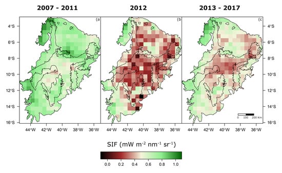
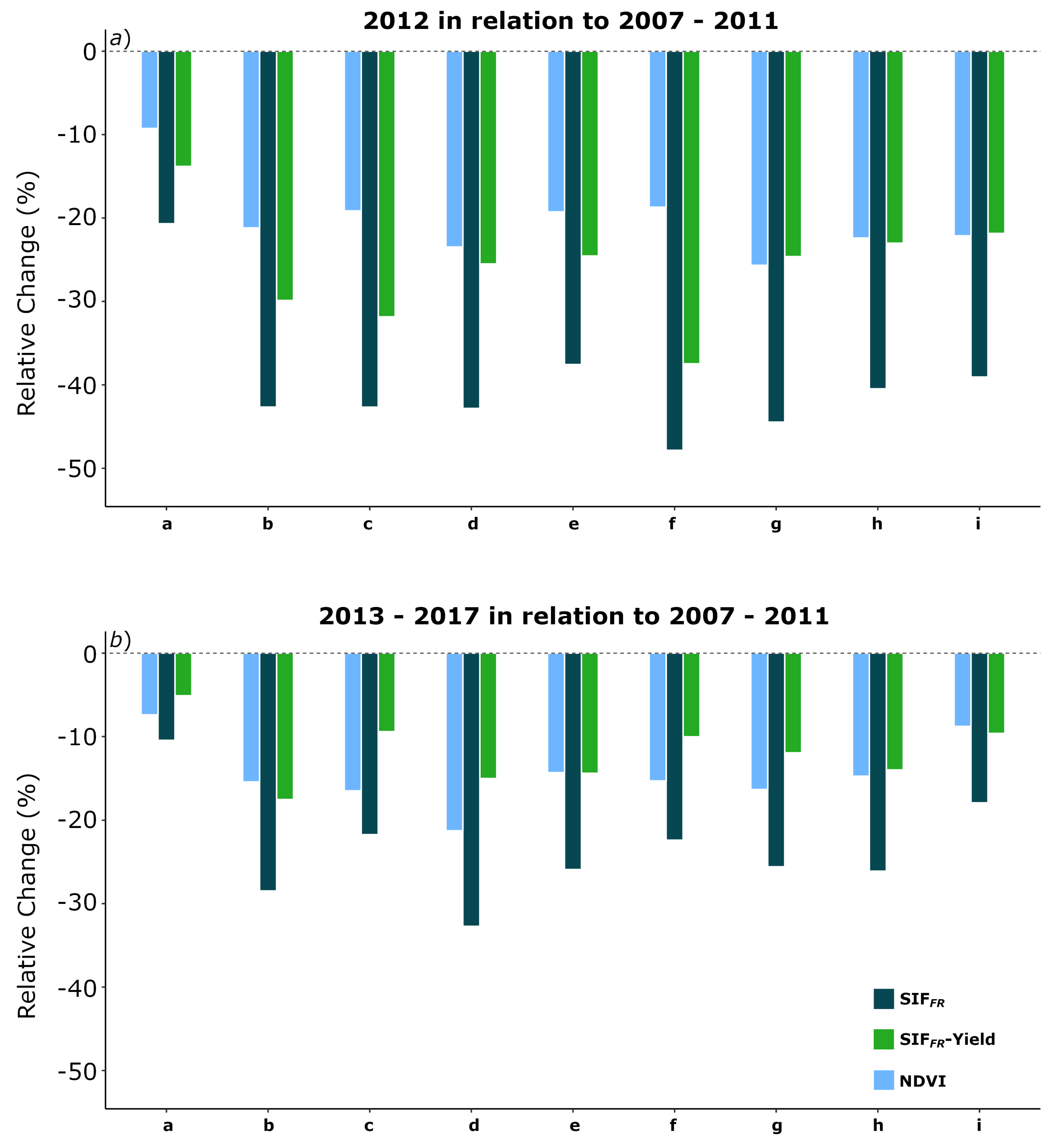
3.4. SIF and Climate: The 2012 Drought

The results of our trend analysis, showing a major drought at the year of 2012 (Figure 5), can be better understood in a spatial analysis subsetting our data into three periods: a more favorable period from 2007 to 2011, a drought period in the year of 2012 and an intermittent-droughts period from 2013 to 2017. The map of average precipitation shows a clear difference among these three periods and give a spatial perspective of the 2012 drought in the studied area (Figure 7). Spatial averages maps of SIF F R , NDVI and their correlation, illustrate the effects of that environmental variation on vegetation biochemistry, structure and photosynthesis (Figure 8, Figure 9 and Figure 10).
Precipitation maps show that the initial period from 2007 to 2011 had more favourable conditions (Figure 7a), while averages for the year of 2012 show a widespread drought in the region (Figure 7b). The subsequent interval from 2013 until 2017 comprised a mix of dry and wet years that was less-favourable than what we observed from 2007 to 2011, if better than 2012 conditions. While the 2012 drought is shown to affect the majority of the Caatinga, dry conditions persisted from 2013 to 2017 particularly at the region’s central area (Figure 7c).
The changes in studied variables observed in the year of 2012, in relation to the period from 2007 to 2011, were large and SIF F R dropped by over 40 % throughout most sites (Figure 11) while NDVI and EVI averages dropped by over 22 % . Even SIF R and SIF F R Yield decreased by over 25 % while Temperature increased by nearly 10 % and Precipitation Rate and Soil Moisture decreased by 54 % and 20 % respectively in 2012, in relation to the previous year’s average. The ratio between red and far-red SIF increased by over 16 % in the year of 2012, with large variation between the different ecoregions of the Caatinga (Figure 11 SIF R / F R ).
The particular response of each ecoregion’s vegetation to the sampled environmental influences can be better observed by comparing the relative change in NDVI (photosynthesis-related structure and biochemistry), SIF F R -Yield (photosynthesis) and their combined response as sampled through SIF F R . Results from 2012 show a marked drop in variables’ means, with vegetation at the Sao Francisco Dunes ecoregion displaying the greatest change in that year among all ecoregions (Figure 12a).
The milder drought period of 2013 to 2017 (as characterized by Figure 5 and Figure 7c) seems to have had a small impact on the Campo Maior ecoregion. Results show that the Northern Sertaneja Depression and the Borborema Plateau were the most affected ecoregions from 2013 to 2017 in relation to what can be observed from 2007 to 2011 (Figure 12b).

4. Discussion

4.1. SIF Responses to Environmental Variation

Fluorescence sampled from Caatinga vegetation seems to vary in similar amplitude as the environmental indicators at the different ecoregions (Figure 4 and Figure 5). The sensitivity of GOME-2 SIF to environmental variation can also be established by observing the results of our Linear Mixed Models (Table 2) and by comparing the relative change observed at the 2012 drought among the various variables (Figure 11) and between NDVI, SIF F R and SIF F R -Yield at each ecoregion (Figure 12). The variables SIF F R -Prod, dSIF F R , SIF F R -SZA and standard SIF F R presented a median drop of more than 40 % during the year of 2012 in relation to the period from 2007 to 2011 (Figure 11). While these variables include the phenological influences of biochemistry and structure on SIF radiative transfer, SIF F R -Yield has had most of these influences removed but it also dropped by a median value of over 25 % in 2012. Considering that both MODIS EVI and NDVI corrected through the MAIAC algorithm have a finer spatial resolution than GOME-2 SIF, it is interesting to see that SIF F R -Yield mean value still dropped by a higher margin than that of the sampled SVIs (Figure 11).
Results from our study show that the interpretation of chlorophyll fluorescence emissions is complex but very informative. As this study demonstrates and as it has been argued in recent reviews [3,11], the main factors to consider for the interpretation of SIF seem to be the resolution and temporal aspect of measurements and the characteristics of the vegetation being measured. Due to the nature of our study and our choice of GOME-2 SIF data, temporal influences in our results could not be controlled and thus, could not be directly tested. Phenology however, consisting of temporal variation on biochemical and structural characteristics of vegetation, has an apparently strong influence on SIF measured at the Caatinga as we will now discuss.

4.2. SIF Seasonality and Phenological Processes

In much of the Caatinga, SIF yearly minimum values were often about a quarter of the yearly maximum values (results not shown), characterizing a large seasonal variation in SIF (Figure 4). For most plants, physiological responses to heat and drought stress generally consist in adaptive measures like: limiting water loss through the closing of stomata and the consequent lowering of the photochemical quenching (qP) and fluorescence emissions [44]; Moreover, dissipating excess-energy through the Non-Photochemical Quenching (NPQ) pathways, which lowers fluorescence emissions, since these processes “compete” for the same energy [4,7,8]. Therefore, the more energy is dissipated through NPQ the less will be left for qP and its associated fluorescence emission. Nonetheless, since we are observing seasonal phenomena, not all variation can be attributed to physiology.
A study testing the effects of the exposure of plants to the combined stresses of drought and high-temperature at the leaf-level reported a five-fold decrease in fluorescence emissions that couldn’t be attributed only to photoadaptive processes such as qP and NPQ but, was instead found to be largely the result of chlorophyll degradation [88]. Similarly, the marked decrease in SIF emissions observed concomitantly with the ecoregion-specific dry seasons (Figure 4) suggests a combined effect of seasonal photosynthesis adaptation (e.g., non-transient lowering of qP and the increasing of NPQ) and phenological processes like chlorophyll degradation and leaf-shedding. These phenological processes are known to play a major role in the Caatinga’s vegetation dynamics [39] and it is reasonable to expect that they must account for much of the observed SIF seasonal variation. This is further supported by the sampled SVI seasonality which adheres closely to SIF seasonality (results not shown) and correlates well to SIF data at most ecoregions (Figure 10 and Appendix A Table A4). Nevertheless, even at the tested monthly scale, these processes are not the exclusive source of SIF output variation as is proven by SIF F R -Yield LMM results (Table 2). While the influences of phenological processes (e.g., leaf flushing, leaf maturation, chlorophyll degradation and leaf shedding) must be considered carefully, our results show that they do not invalidate the interpretation of chlorophyll fluorescence seasonality and stress responses.
Furthermore, the reversal in SIF F R and SIF R emission levels observed at the onset of the dry season (Figure 4) is consistent with the expected effects of leaf shedding and chlorophyll degradation on the reabsoption of SIF R [14,15] but, this effect is shown here with fluorescence emitted by a large sample of plants instead of that emitted by a single leaf as described by Buschmann [13]. To our knowledge, this is the only study showing the relationship between the SIF R / F R ratio and chlorophyll content at the community level in the seasonal scale, as it is demonstrated by the seasonality of SIF F R and SIF R emission levels (Figure 4), and also demonstrated at an anomalous drought by our trend analysis (Figure 5, year 2012). However, LMM results show that SIF R / F R variation is mostly driven by the phenological cycle as the effect of seasonality was constrained in our models though random factors and SIF R / F R was not significantly affected by any fixed factor (Table 2).

4.3. Apparent Influence of Vegetation Differences in SIF Responses

Land cover analysis through ESA’s GlobCover 2009 product agrees with the previously described dominance of shrublands and open forest physiognomies at the Caatinga area, as described by major biogeographic studies [37,89]. The prevalence of crop-related classes (mosaic classes, Figure 3 and Appendix A Table A1 and Table A2) is supported by the previously reported presence of subsistence agriculture with little or no irrigation at the Caatinga [36,40]. This simple land cover analysis supports our assumptions that Caatinga vegetation is a mosaic of diverse physiognomies, including widespread human occupation and land cover by subsistence agriculture, and shows that the ecoregions identified within the Caatinga [35] are different concerning not only geomorphology, climate and soil but also in their vegetation (Figure 3 and Appendix A Table A1 and Table A2).
Our results suggest that vegetation types and their particular characteristics significantly influence the observed seasonality of SIF and its apparent responses to abiotic stress (Table 4). We suggest that such influences might help to explain why some of our results seem counter-intuitive, or discrepant. For example, the seasonality of SIF F R and SIF R at the Ibiapaba-Araripe Complex ecoregion shows a discrepant pattern with a very small seasonal variation in SIF R that doesn’t seem comparable to that of SIF F R at that same region (Figure 4c). While we could speculate on differences in local vegetation composition (e.g., more presence of cacti, differences in deciduousness between vegetation strata) between the local types and those at other regions, we do not know the reasons for this particular discrepancy.
Furthermore, we have also observed considerable differences in the correlation of SIF and SVIs between different areas of the Caatinga (Figure 10 and Appendix A Table A4). Considering the nature of these data we suggest that temporal differences in responses to environmental variation must influence the observed correlation discrepancies since, while SIF can respond near instantly to environmental constraints SVIs will depend on slower biosynthesis and conversion of pigments and on similarly slow structural changes (Figure 11). Daily cycles of environmental variation and seasonal change in the ranges of such daily environmental variation have been already been shown to influence chlorophyll fluorescence output in temperate vegetation [90] as well as in the tropical semiarid vegetation of Caatinga [91]. Therefore, the time of day when measurements are made is greatly significant for the interpretation of SIF but not for the interpretation of vegetation indices like EVI and NDVI. Thus, we suggest that daily maxima of SIF should be more directly comparable to vegetation indices in the context of seasonal studies. Nevertheless, considering the spatial pattern observed in the correlation between SIF and NDVI (Figure 10) and how that matches the long term ecoregion-specific correlation discrepancies (Appendix A Table A4), we believe it is likely that vegetation structure and composition are also influencing these results.
Despite such uncertainties, the reliability of satellite measurements of SIF is further illustrated by the coherence of LMM slopes and land cover classification data. As our results have shown, the higher the percentage of the ecoregion’s vegetation was classified as forest, the weaker was that ecoregion’s response to tested environmental variables (Table 4). This is reasonable considering that the environmental factors modelled in LMMs were soil moisture and surface temperature (related to variations in water availability and vapour pressure deficit effects on vegetation) and that root depths in forest physiognomies are greater and also that moisture is conserved in the system due its structural characteristics [44]. Thus, denser and taller vegetation has greater resistance to drought effects (i.e., weaker response to changes in soil moisture at the measured depth) if compared to shorter physiognomies such as shrublands and savannas: this is an emergent property of forest ecosystems and it is closely related to the concept of ecosystem resilience [92,93]. Furthermore, the observed correlations between GlobCover physiognomies and response to environmental variables were greater with SIF F R than with SIF F R -Yield, in agreement with our assumptions regarding the expected effects of normalizing SIF by a structure and biochemistry vegetation proxy like NDVI. This is, to our knowledge, the first study to show results substantiating an emergent ecosystem property through remotely sensed measurements of chlorophyll fluorescence.
Considering the consistency of SIF responses with observed climate, we believe that our study did not suffer from the limitation of using land cover data from a single year in reference to SIF and other reflectance data from an eleven year period. However, this limitation and the mixed representativeness of GOME-2’s large pixels, preclude a more detailed discussion of SIF results in relation to the emitting vegetation. More studies using higher-definition SIF data (i.e., with other instruments like OCO-2, TanSat, TROPOMI, OCO-3 or the upcoming FLEX) accompanied by more precise land cover data, should be employed to advance knowledge of vegetation ecophysiological responses.

4.4. Linear Mixed Models and Our Adjustments to SIF

The LMM model using SIF F R -SZA, the normalization of SIF F R values by the cosine of the Solar Zenith Angle (SZA), effectively improved SIF’s relationship to environmental data (Table 3, slightly higher marginal R 2 and considerably lower RMSE, REML and BIC). These results contrast with conclusions from previous studies suggesting that SZA normalization could amplify noise if applied to measurements taken from lower intensity emissions (as observed at the Caatinga) and influence perceived sun/shade effects [29]. Furthermore, it is interesting to notice that our study region is under direct influence from the South Atlantic Anomaly (SAA) and it is, therefore, inherently noisy and perhaps a “worst-case scenario” for SZA normalization (see PAR normalization in Joiner et al. [28]).
The SIF F R -Prod adjustment, based on the classic productivity equation of Monteith and Moss [62,63], already shown in a preliminary study to increase the correlation between GOME-2 SIF and FLUXNET GPP across diverse vegetation types [66], yielded significant improvements on LMM goodness-of-fit in relation to standard SIF (Table 3). However, due to the substantial increase it caused in the effect size of the Ecoregion factor on tested LMMs (Table 2) and, considering that this effect encapsulates part of the structural variability between the different ecoregions, we conjecture that SIF F R -Prod may be “double-counting” the influence of emitting vegetation as it is calculated by multiplying SIF by NDVI and both variables are strongly influenced by vegetation structure and biochemistry. This is also suggested by the fact that although the SIF F R -Prod LMM had the highest coefficients of determination, it had relatively worse quality than what was observed with the SIF F R -SZA LMM (Table 3, RMSE, REML and BIC are higher for SIF F R -Prod than for the SIF F R -SZA LMM).
The spectral adjustment here called SIF F R -Yield, consisting on dividing the observed GOME-2 SIF by corresponding NDVI, had the largest effect on SIF among the tested modifications (Table 2 and Table 3). The observed decrease in goodness-of-fit of the SIF F R -Yield LMM in relation to models using SIF F R , dSIF F R , SIF F R -SZA and SIF F R -Prod is in agreement with the hypothesis that SIF F R -Yield normalizes SIF data according to biochemistry and structure as sampled by NDVI, removing much of these influences from SIF data in the proportion to which NDVI is able to capture them. Because in our LMMs the Ecoregion factor encapsulates all unmodelled differences between the sampled vegetation at the different ecoregions, the drop in relative effect of that factor in relation to environmental factors Temperature and Soil Moisture in Yield-normalized models (Table 2) shows that much of these unmodelled differences concern biochemical and structural influences on GOME-2 SIF data. Certainly NDVI would not be an adequate proxy to biochemistry- and structure-related effects on SIF emissions for all types of vegetation but, it is worth noting that NDVI at the Caatinga is not subject to strong saturation effects and it seldom rises above 0.7 in the majority of the region (Figure 9). We suggest that Yield-normalization is necessary for interpreting fluorescence measurements as our results show that SIF-Yield adds another perspective on SIF measurements (Figure 12), separating the long-term effects of phenology, biochemistry and structure (related to photosynthetic capacity) from the transient photosynthetic rate-related effects (related to photosynthetic performance).
Therefore, our findings support previous suggestions that SIF has potential to improve our understanding of plant responses to drought [30,31,32] and exemplify in a case study the premise that SIF can be more informative when combined with vegetation indices.

5. Conclusions

In this study of the semiarid Caatinga vegetation of northeast Brazil, we attempted to characterize eleven years of Sun-induced chlorophyll fluorescence (SIF) seasonality (from 2007 to 2017) and SIF responses to a major drought in 2012. To achieve these objectives we adjusted SIF through combination with NDVI and also used angular adjustments to SIF provided with original GOME-2 data. Original and modified SIF measures were tested against environmental data using time-series decomposition, rank correlation tests and linear mixed models (LMMs).
Results demonstrated that seasonal variation and drought responses of adjusted SIF emissions at the community/landscape level correspond to previously reported leaf-level physiological responses. These observations are more relevant since they include both red and far-red SIF, as well as their ratio, and they were made in the complex and heterogeneously structured plant communities of the semiarid Caatinga of northeast Brazil. Our results with angular and spectral adjustments to SIF, although partially implemented with geometrically and radiometrically incompatible data (GOME-2 SIF and MODIS MAIAC SVIs), suggest that many of the assumptions behind the tested adjustments are likely correct. Our findings are relevant considering GOME-2 SIF’s low spatial resolution and the noise inherent to measurements taken from this area due to the South Atlantic Anomaly. Here we show for the first time that environmental responses measured through adjusted GOME-2 SIF correlate with a known emergent ecosystem property (resilience), illustrating its value for ecological studies of vegetation.
We suggest that more studies testing angular and spectral adjustments to SIF using higher definition SIF data in combination with other reflectance data are necessary to improve our understanding of landscape-level vegetation responses. Furthermore, continuous chlorophyll fluorescence measurements from tower-based instruments and coordinated field campaigns are recommended to increase our understanding of vegetation ecophysiological responses at different scales, to validate our findings and to allow predictions of possible ecological shifts resulting from the ongoing global climate change.

Author Contributions

Conceptualization, E.B. and F.P.; methodology, E.B.; software, E.B. and R.D.; formal analysis, E.B.; resources, F.P. and D.V.; data curation, E.B. and R.D.; writing—original draft preparation, E.B.; writing—review and editing, E.B., R.D., F.P. and D.V.; supervision, F.P. and D.V.; funding acquisition, E.B., R.D., F.P. and D.V. All authors have read and agreed to the published version of the manuscript.

Funding

This research was funded by the PCI program of CNPq, the Brazilian National Council of Research, grant number 313142/2016-5, and by the São Paulo Research Foundation (FAPESP), grant 2015/22987-7 and by the Foundation for Science and Application of Space Technology (FUNCATE).

Acknowledgments

The authors thank Luis Guanter for his comments and suggestions on this manuscript, Rob J Hyndman for his instrumental advice on time-series analysis, NASA for the freely available data, Alexei Lyapustin and his team for the MODIS-MAIAC corrections, Flora Martins for the helpful discussion and the Foundation for Science and Application of Space Technology (FUNCATE) for its support.

Conflicts of Interest

The authors declare no conflict of interest. The funders had no role in the design of the study; in the collection, analyses, or interpretation of data; in the writing of the manuscript, or in the decision to publish the results.

Appendix A

Figure A1. Data trends of SIF F R , NDVI and EVI, from February 2007 to December 2017. Trends obtained from time-series decomposition with Locally Estimated Scatterplot Smoothing (LOESS). SIF F R is Sun-Induced Fluorescence from GOME-2 at the far-red peak. NDVI is MODIS MAIAC NDVI and EVI is MODIS MAIAC EVI. All graphs have the same axis ranges for all variables.
Remotesensing 12 03264 g0a1
Table A1. GlobCover 2009 land cover classification system codes and names correspondence table for the Caatinga of northeast Brazil.
Class NumberClass Name
14Rainfed croplands
20Mosaic cropland (50–70%)/vegetation (grassland/shrubland/forest) (20–50%)
30Mosaic vegetation (grassland/shrubland/forest) (50–70%)/cropland (20–50%)
40Closed to open (>15%) broadleaved evergreen or semi-deciduous forest (>5 m)
50Closed (>40%) broadleaved deciduous forest (>5 m)
60Open (15–40%) broadleaved deciduous forest/woodland (>5 m)
110Mosaic forest or shrubland (50–70%)/grassland (20–50%)
120Mosaic grassland (50–70%)/forest or shrubland (20–50%)
130Closed to open (>15%) (broadleaved or needleleaved, evergreen or deciduous) shrubland (<5 m)
140Closed to open (>15%) herbaceous vegetation (grassland, savannas or lichens/mosses)
150Sparse (<15%) vegetation
160Closed to open (>15%) broadleaved forest regularly flooded (semi-permanently or temporarily)
170Closed (>40%) broadleaved forest or shrubland permanently flooded
180Closed to open (>15%) grassland or woody vegetation on regularly flooded or waterlogged soil
190Artificial surfaces and associated areas (Urban areas >50%)
200Bare areas
210Water bodies
Table A2. Relative cover per Ecoregion from ESA’s GlobCover 2009—values represent percentages per ecoregion. Codes represent land cover types listed in Table A1. Ecoregions are represented by letter according to the following list: (a) Campo Maior; (b) Northern Sertaneja Depression; (c) Araripe-Ibiapaba Complex; (d) Borborema Plateau; (e) Major Southern Sertaneja Depression; (f) Sao Francisco Dunes; (g) Raso da Catarina; (h) Minor Southern Sertaneja Depression; (i) Chapada Diamantina. Numbers have been rounded to facilitate reading.
Class Number Ecoregion
abcdefghi
140.7017.653.5821.1512.762.9924.8428.707.13
208.5216.5419.9212.7629.9637.9914.7321.4521.74
3020.6729.3614.6628.7322.9711.2429.4931.5126.72
409.192.034.350.835.025.020.920.608.91
500.430.960.880.833.081.861.730.326.58
600.352.513.640.264.505.480.320.025.45
1100.629.330.9010.722.900.723.855.793.91
1200.010.280.020.150.270.370.370.300.69
13059.2519.9951.9624.0117.5827.4321.329.6117.80
1400.01
1500.010.200.010.070.070.580.080.080.30
1600.010.01
1700.01
1800.100.010.010.010.30
1900.090.010.120.020.010.05
2000.010.300.040.210.470.720.580.550.26
2100.130.750.030.160.385.591.761.030.20
Table A3. Linear Mixed Models’ Random Effect Variances—SIF F R is Sun-Induced Fluorescence at the far-red peak; dSIF F R is the daily average of SIF based on a clear sky PAR proxy; SIF F R -Prod is the product of SIF F R by NDVI; SIF F R SZA is the quotient of SIF F R by the cosine of the Sun’s Zenith Angle (SZA); SIF F R Yield is the quotient of SIF F R by NDVI; For all SIF F R models: n = 1179 ; M o n t h = 12 ; Month:Year = 131. SIF R is Sun-Induced Fluorescence at the red peak; SIF R / F R is the ratio between SIF R and SIF F R . For the two models involving SIF R : n = 747 ; M o n t h = 12 ; Month:Year = 83.
SIF FR dSIF FR SIF FR -ProdSIF FR -SZASIF FR -YieldSIF R SIF R / FR
EffectVarianceVarianceVarianceVarianceVarianceVarianceVariance
Month:Year0.0460.0530.0480.0110.0490.0730.006
Month0.1610.1920.1290.0210.2180.1720.017
residual0.1460.1480.1040.0280.2770.2180.985
Table A4. τ (tau) correlation rank from Kendall’s Correlation tests between SIF and SVIs by Ecoregion and for the whole Caatinga. SIF F R is Sun-Induced Fluorescence at the far-red peak, EVI is the Enhanced Vegetation Index and NDVI is the Normalized Difference Vegetation Index. For SIF F R tests: n = 131 pairs for each ecoregion and n = 1179 pairs for Caatinga; SIF R is Sun-Induced Fluorescence at the red peak; For SIF R tests: n = 59 pairs for each ecoregion and n = 531 pairs for Caatinga; Region letters are the ecoregions as in Figure 1: (a) Campo Maior; (b) Northern Sertaneja Depression; (c) Araripe-Ibiapaba Complex; (d) Borborema Plateau; (e) Major Southern Sertaneja Depression; (f) Sao Francisco Dunes; (g) Raso da Catarina; (h) Minor Southern Sertaneja Depression; (i) Chapada Diamantina. Asterisks denote significance levels: *** represents p value < 0.001.
RegionSIF FR and EVISIF FR and NDVISIF R and EVISIF R and NDVI
a0.42 ***0.47 ***0.25 ***0.26 ***
b0.72 ***0.73 ***0.65 ***0.68 ***
c0.54 ***0.57 ***0.50 ***0.59 ***
d0.70 ***0.71 ***0.54 ***0.54 ***
e0.65 ***0.65 ***0.54 ***0.56 ***
f0.58 ***0.59 ***0.37 ***0.42 ***
g0.64 ***0.64 ***0.28 ***0.30 ***
h0.46 ***0.47 ***0.31 ***0.34 ***
i0.42 ***0.44 ***0.25 ***0.25 ***
Caatinga0.57 ***0.58 ***0.41 ***0.43 ***

References

  1. Sellers, P.J.; Schimel, D.S.; Moore, B.; Liu, J.; Eldering, A. Observing carbon cycle–climate feedbacks from space. Proc. Natl. Acad. Sci. USA 2018, 115, 7860–7868. [Google Scholar] [CrossRef] [PubMed] [Green Version]
  2. Porcar-Castell, A.; Tyystjärvi, E.; Atherton, J.; Van Der Tol, C.; Flexas, J.; Pfündel, E.E.; Moreno, J.; Frankenberg, C.; Berry, J.A. Linking chlorophyll a fluorescence to photosynthesis for remote sensing applications: Mechanisms and challenges. J. Exp. Bot. 2014, 65, 4065–4095. [Google Scholar] [CrossRef] [PubMed]
  3. Mohammed, G.H.; Colombo, R.; Middleton, E.M.; Rascher, U.; van der Tol, C.; Nedbal, L.; Goulas, Y.; Pérez-Priego, O.; Damm, A.; Meroni, M.; et al. Remote sensing of solar-induced chlorophyll fluorescence (SIF) in vegetation: 50 years of progress. Remote Sens. Environ. 2019, 231, 111177. [Google Scholar] [CrossRef]
  4. Butler, W.L. Energy Distribution in the Photochemical Apparatus of Photosynthesis. Annu. Rev. Plant Physiol. 1978, 29, 345–378. [Google Scholar] [CrossRef]
  5. Demmig-Adams, B.; Adams, W.W. Photoprotection and Other Responses of Plants to High Light Stress. Annu. Rev. Plant Physiol. Plant Mol. Biol. 1992, 43, 599–626. [Google Scholar] [CrossRef]
  6. Demmig-Adams, B.; Adams, W.W. Xanthophyll cycle and light stress in nature: Uniform response to excess direct sunlight among higher plant species. Planta 1996, 198, 460–470. [Google Scholar] [CrossRef]
  7. Maxwell, K.; Johnson, G.N. Chlorophyll fluorescence—A practical guide. J. Exp. Bot. 2000, 51, 659–668. [Google Scholar] [CrossRef] [PubMed]
  8. Baker, N.R. Chlorophyll Fluorescence: A Probe of Photosynthesis In Vivo. Annu. Rev. Plant Biol. 2008, 59, 89–113. [Google Scholar] [CrossRef] [Green Version]
  9. Govindje, E. Sixty-three years since Kautsky: Chlorophyll a Fluorescence. Aust. J. Plant Physiol. 1995, 22, 131–160. [Google Scholar] [CrossRef]
  10. Meroni, M.; Rossini, M.; Guanter, L.; Alonso, L.; Rascher, U.; Colombo, R.; Moreno, J. Remote sensing of solar-induced chlorophyll fluorescence: Review of methods and applications. Remote Sens. Environ. 2009, 113, 2037–2051. [Google Scholar] [CrossRef]
  11. Ryu, Y.; Berry, J.A.; Baldocchi, D.D. What is global photosynthesis? History, uncertainties and opportunities. Remote Sens. Environ. 2019, 223, 95–114. [Google Scholar] [CrossRef]
  12. Malenovský, Z.; Mishra, K.B.; Zemek, F.; Rascher, U.; Nedbal, L. Scientific and technical challenges in remote sensing of plant canopy reflectance and fluorescence. J. Exp. Bot. 2009, 60, 2987–3004. [Google Scholar] [CrossRef] [PubMed] [Green Version]
  13. Buschmann, C. Variability and application of the chlorophyll fluorescence emission ratio red/far-red of leaves. Photosynth. Res. 2007, 92, 261–271. [Google Scholar] [CrossRef] [PubMed]
  14. Rossini, M.; Nedbal, L.; Guanter, L.; Ac, A.; Alonso, L.; Burkart, A.; Cogliati, S.; Colombo, R.; Damm, A.; Drusch, M.; et al. Red and far red Sun-induced chlorophyll fluorescence as a measure of plant photosynthesis. Geophys. Res. Lett. 2015, 42, 1632–1639. [Google Scholar] [CrossRef] [Green Version]
  15. Van Wittenberghe, S.; Alonso, L.; Verrelst, J.; Moreno, J.; Samson, R. Bidirectional sun-induced chlorophyll fluorescence emission is influenced by leaf structure and light scattering properties—A bottom-up approach. Remote Sens. Environ. 2015, 158, 169–179. [Google Scholar] [CrossRef]
  16. Ač, A.; Malenovský, Z.; Olejníčková, J.; Gallé, A.; Rascher, U.; Mohammed, G. Meta-analysis assessing potential of steady-state chlorophyll fluorescence for remote sensing detection of plant water, temperature and nitrogen stress. Remote Sens. Environ. 2015, 168, 420–436. [Google Scholar] [CrossRef] [Green Version]
  17. Fournier, A.; Daumard, F.; Champagne, S.; Ounis, A.; Goulas, Y.; Moya, I. Effect of canopy structure on sun-induced chlorophyll fluorescence. ISPRS J. Photogramm. Remote Sens. 2012, 68, 112–120. [Google Scholar] [CrossRef]
  18. Verrelst, J.; Rivera, J.P.; van der Tol, C.; Magnani, F.; Mohammed, G.; Moreno, J. Global sensitivity analysis of the SCOPE model: What drives simulated canopy-leaving sun-induced fluorescence? Remote Sens. Environ. 2015, 166, 8–21. [Google Scholar] [CrossRef]
  19. Tucker, C.J. Red and Photographic Infrared Linear Combinations for Monitoring Vegetation. Remote Sens. Environ. 1979, 8, 127–150. [Google Scholar] [CrossRef] [Green Version]
  20. Huete, A.R.; Liu, H.; Batchily, K.; Van Leeuwen, W. A comparison of vegetation indices global set of TM images for EOS-MODIS. Remote Sens. Environ. 1997, 59, 440–451. [Google Scholar] [CrossRef]
  21. Huete, A.R.; Justice, C.; Leeuwen, W. MODIS Vegetation Index (MOD 13): Algorithm Theoretical Basis Document, version 3; Technical Report; NASA: Washington, DC, USA, 1999. [Google Scholar]
  22. Bannari, A.; Morin, D.; Bonn, F.; Huete, A.R. A review of vegetation indices. Remote Sens. Rev. 1995, 13, 95–120. [Google Scholar] [CrossRef]
  23. Entcheva-Campbell, P.; Middleton, E.; Corp, L.; Kim, M. Contribution of chlorophyll fluorescence to the apparent vegetation reflectance. Sci. Total. Environ. 2008, 404, 433–439. [Google Scholar] [CrossRef] [PubMed]
  24. Calderón, R.; Navas-Cortés, J.; Lucena, C.; Zarco-Tejada, P. High-resolution airborne hyperspectral and thermal imagery for early detection of Verticillium wilt of olive using fluorescence, temperature and narrow-band spectral indices. Remote Sens. Environ. 2013, 139, 231–245. [Google Scholar] [CrossRef]
  25. Yang, P.; van der Tol, C.; Verhoef, W.; Damm, A.; Schickling, A.; Kraska, T.; Muller, O.; Rascher, U. Using reflectance to explain vegetation biochemical and structural effects on sun-induced chlorophyll fluorescence. Remote Sens. Environ. 2018, 231, 110996. [Google Scholar] [CrossRef]
  26. Gitelson, A.; Buschmann, C.; Lichtenthaler, H.K. Leaf chlorophyll fluorescence corrected for re-absorption by means of absorption and reflectance measurements. J. Plant Physiol. 1998, 152, 283–296. [Google Scholar] [CrossRef]
  27. Joiner, J.; Guanter, L.; Lindstrot, R.; Voigt, M.; Vasilkov, A.P.; Middleton, E.M.; Huemmrich, K.F.; Yoshida, Y.; Frankenberg, C. Global monitoring of terrestrial chlorophyll fluorescence from moderate-spectral-resolution near-infrared satellite measurements: Methodology, simulations, and application to GOME-2. Atmos. Meas. Tech. 2013, 6, 2803–2823. [Google Scholar] [CrossRef] [Green Version]
  28. Joiner, J.; Yoshida, Y.; Guanter, L.; Middleton, E.M. New methods for retrieval of chlorophyll red fluorescence from hyper-spectral satellite instruments: Simulations and application to GOME-2 and SCIAMACHY. Atmos. Meas. Tech. Discuss. 2016, 9, 3939–3967. [Google Scholar] [CrossRef] [Green Version]
  29. Köhler, P.; Guanter, L.; Kobayashi, H.; Walther, S.; Yang, W. Assessing the potential of sun-induced fluorescence and the canopy scattering coefficient to track large-scale vegetation dynamics in Amazon forests. Remote Sens. Environ. 2018, 204, 769–785. [Google Scholar] [CrossRef] [Green Version]
  30. Sun, Y.; Fu, R.; Dickinson, R.; Joiner, J.; Frankenberg, C.; Gu, L.; Xia, Y.; Fernando, N. Drought onset mechanisms revealed by satellite solar-induced chlorophyll fluorescence: Insights from two contrasting extreme events. J. Geophys. Res. Biogeosci. 2015, 120, 2427–2440. [Google Scholar] [CrossRef]
  31. Yoshida, Y.; Joiner, J.; Tucker, C.; Berry, J.; Lee, J.E.; Walker, G.; Reichle, R.; Koster, R.; Lyapustin, A.; Wang, Y. The 2010 Russian drought impact on satellite measurements of solar-induced chlorophyll fluorescence: Insights from modeling and comparisons with parameters derived from satellite reflectances. Remote Sens. Environ. 2015, 166, 163–177. [Google Scholar] [CrossRef]
  32. Wang, S.; Huang, C.; Zhang, L.; Lin, Y.; Cen, Y.; Wu, T. Monitoring and assessing the 2012 drought in the great plains: Analyzing satellite-retrieved solar-induced chlorophyll fluorescence, drought indices, and gross primary production. Remote Sens. 2016, 8, 61. [Google Scholar] [CrossRef] [Green Version]
  33. Jiao, W.; Chang, Q.; Wang, L. The sensitivity of satellite solar-induced chlorophyll fluorescence (SIF) to meteorological drought. Earth Future 2019, 7, 558–573. [Google Scholar]
  34. Cunha, A.P.; Alvalá, R.C.; Nobre, C.A.; Carvalho, M.A. Monitoring vegetative drought dynamics in the Brazilian semiarid region. Agric. For. Meteorol. 2015, 214–215, 494–505. [Google Scholar] [CrossRef]
  35. Velloso, A.L.; Sampaio, E.V.S.B.; Pareyn, F.G.C. (Eds.) Ecoregiões Propostas Para o Bioma Caatinga (in Portuguese), 2nd ed.; Associação Plantas do Nordeste; Instituto de Conservação Ambiental—The Nature Conservancy do Brasil: Recife, Brazil, 2002; p. 75. [Google Scholar]
  36. Silva, J.M.C.; Leal, I.R.; Tabarelli, M. (Eds.) Caatinga—The Largest Tropical Dry Forest Region in South America; Springer International Publishing: Cham, Switzerland, 2017; p. 482. [Google Scholar]
  37. Andrade-Lima, D. The Caatingas Domain (original article in English). Revista Brasileira Botânica 1981, 4, 149–162. [Google Scholar]
  38. Breckle, S.W. Walter’s Vegetation of the Earth, 4th ed.; Springer: Berlin/Heidelberg, Germany, 2002; p. 525. [Google Scholar]
  39. Pennington, R.; Prado, D.E.; Pendry, C. Neotropical Seasonally Dry Forests and Quaternary Vegetation Changes. J. Biogeogr. 2000, 27, 261–273. [Google Scholar] [CrossRef]
  40. Pennington, R.; Lehmann, C.E.R.; Rowland, L.M. Tropical savannas and dry forests. Curr. Biol. 2018, 28, 542–545. [Google Scholar] [CrossRef] [Green Version]
  41. Santos, J.C.; Leal, I.R.; Almeida-Cortez, J.S.; Fernandes, G.W.; Tabarelli, M. Caatinga: The Scientific Negligence Experienced by a Dry Tropical Forest. Trop. Conserv. Sci. 2011, 4, 276–286. [Google Scholar] [CrossRef]
  42. Zscheischler, J.; Mahecha, M.D.; Harmeling, S.; Rammig, a.; Tomelleri, E.; Reichstein, M. Extreme events in gross primary production: A characterization across continents. Biogeosci. Discuss. 2014, 11, 1869–1907. [Google Scholar] [CrossRef] [Green Version]
  43. Zscheischler, J.; Mahecha, M.D.; Avitabile, V.; Calle, L.; Carvalhais, N.; Ciais, P.; Gans, F.; Gruber, N.; Hartmann, J.; Herold, M.; et al. Reviews and syntheses: An empirical spatiotemporal description of the global surface-atmosphere carbon fluxes: Opportunities and data limitations. Biogeosciences 2017, 14, 3685–3703. [Google Scholar] [CrossRef] [Green Version]
  44. Larcher, W. Physiological Plant Ecology, 4th ed.; Springer: Berlin/Heidelberg, 2003; p. 514. [Google Scholar]
  45. Arino, O.; Ramos Perez, J.J.; Kalogirou, V.; Bontemps, S.; Defourny, P.; Van Bogaert, E. Global Land Cover Map for 2009 (GlobCover 2009). European Space Agency (ESA) and Universite catholique de Louvain (UCL), PANGAEA. 2012. Available online: https://doi.org/doi:10.1002/9781118786352.wbieg0878 (accessed on 10 June 2019).
  46. Wan, Z.; Hook, S.; Hulley, G. MOD11C3 MODIS/Terra Land Surface Temperature/Emissivity Monthly L3 Global 0.05Deg CMG V006. 2015. Distributed by NASA EOSDIS Land Processes DAAC. Available online: https://doi.org/10.5067/MODIS/MOD11C3.006 (accessed on 5 August 2018).
  47. TRMM (TMPA/3B43) Rainfall Estimate L3 1 Month 0.25 Degree x 0.25 Degree V7. 2011. Available online: https://doi.org/10.5067/TRMM/TMPA/MONTH/7 (accessed on 6 August 2018).
  48. Parker, J.A.; Kenyon, R.V.; Troxel, D.E. Comparison of Interpolating Methods for Image Resampling. IEEE Trans. Med. Imaging 1983, 2, 31–39. [Google Scholar] [CrossRef]
  49. Zhu, A.X. Resampling, Raster. In International Encyclopedia of Geography: People, the Earth, Environment and Technology; Richardson, D., Castree, N., Goodchild, M.F., Kobayashi, A., Liu, W., Marston, R.A., Eds.; Wiley Online Library: Hoboken, NJ, USA, 2017. [Google Scholar] [CrossRef]
  50. Dorigo, W.; Wagner, W.; Albergel, C.; Albrecht, F.; Balsamo, G.; Brocca, L.; Chung, D.; Ertl, M.; Forkel, M.; Gruber, A.; et al. ESA CCI Soil Moisture for improved Earth system understanding: State-of-the art and future directions. Remote Sens. Environ. 2017, 203, 185–215. [Google Scholar] [CrossRef]
  51. Lyapustin, A.I.; Wang, Y. MCD19A1 MODIS/Terra+Aqua Land Surface BRF Daily L2G Global 500 m and 1 km SIN Grid V006. 2018, distributed by NASA EOSDIS Land Processes DAAC. Available online: https://doi.org/10.5067/MODIS/MCD19A1.006 (accessed on 2 June 2019).
  52. Lyapustin, A.I.; Wang, Y.; Laszlo, I.; Hilker, T.; Hall, F.G.; Sellers, P.J.; Tucker, C.J.; Korkin, S.V. Multi-angle implementation of atmospheric correction for MODIS (MAIAC): 3. Atmospheric correction. Remote Sens. Environ. 2012, 127, 385–393. [Google Scholar] [CrossRef]
  53. Dalagnol, R.; Wagner, F.H.; Galvão, L.S.; Nelson, B.W.; De Aragão, L.E.O.E. Life cycle of bamboo in the southwestern Amazon and its relation to fire events. Biogeosciences 2018, 15, 6087–6104. [Google Scholar] [CrossRef] [Green Version]
  54. Frankenberg, C.; O’Dell, C.; Berry, J.; Guanter, L.; Joiner, J.; Köhler, P.; Pollock, R.; Taylor, T.E. Prospects for chlorophyll fluorescence remote sensing from the Orbiting Carbon Observatory-2. Remote Sens. Environ. 2014, 147, 1–12. [Google Scholar] [CrossRef] [Green Version]
  55. Köehler, P.; Frankenberg, C.; Magney, T.S.; Guanter, L.; Joiner, J.; Landgraf, J. Global retrievals of solar induced chlorophyll fluorescence with TROPOMI: First results and inter-sensor comparison to OCO-2. Geophys. Res. Lett. 2018, 45, 10456–10463. [Google Scholar] [CrossRef] [Green Version]
  56. Du, S.; Liu, L.; Liu, X.; Zhang, X.; Zhang, X.; Bi, Y.; Zhang, L. Retrieval of global terrestrial solar-induced chlorophyll fluorescence from TanSat satellite. Sci. Bull. 2018, 63, 1502–1512. [Google Scholar] [CrossRef] [Green Version]
  57. Joiner, J.; Yoshida, Y.; Vasilkov, A.P.; Middleton, E.M.; Campbell, P.K.; Yoshida, Y.; Kuze, A.; Corp, L.A. Filling-in of near-infrared solar lines by terrestrial fluorescence and other geophysical effects: Simulations and space-based observations from SCIAMACHY and GOSAT. Atmos. Meas. Tech. 2012, 5, 809–829. [Google Scholar] [CrossRef] [Green Version]
  58. Tilstra, L.G.; Tuinder, O.N.E.; Stammes, P. A New Method for in-Flight Degradation Correction of GOME-2 Earth Reflectance Measurements, with Application to the Absorbing Aerosol Index; Technical Report; EUMETSAT: Darmstadt, Germany, 2012. [Google Scholar]
  59. Miao, G.; Guan, K.; Yang, X.; Bernacchi, C.J.; Berry, J.A.; DeLucia, E.H.; Wu, J.; Moore, C.E.; Meacham, K.; Cai, Y.; et al. Sun-Induced Chlorophyll Fluorescence, Photosynthesis, and Light Use Efficiency of a Soybean Field from Seasonally Continuous Measurements. J. Geophys. Res. Biogeosci. 2018, 123, 610–623. [Google Scholar] [CrossRef]
  60. Verma, M.; Schimel, D.; Evans, B.; Frankenberg, C.; Beringer, J.; Drewry, D.; Magney, T.; Marang, I.; Hutley, L.; Moore, C.; et al. Effect of environmental conditions on the relationship between solar-induced fluorescence and gross primary productivity at an OzFlux grassland site. J. Geophys. Res. Biogeosci. 2018, 122, 716–733. [Google Scholar] [CrossRef] [Green Version]
  61. Sellers, P.; Berry, J.; Collatz, G.; Field, C.; Hall, F. Canopy reflectance, photosynthesis, and transpiration. III. A reanalysis using improved leaf models and a new canopy integration scheme. Remote Sens. Environ. 2003, 42, 187–216. [Google Scholar] [CrossRef]
  62. Monteith, J.L. Solar Radiation and Productivity in Tropical Ecosystems. J. Appl. Ecol. 1972, 9, 747. [Google Scholar] [CrossRef] [Green Version]
  63. Monteith, J.L.; Moss, C.J. Climate and the Efficiency of Crop Production in Britain. Philos. Trans. R. Soc. B Biol. Sci. 1977, 281, 277–294. [Google Scholar]
  64. Gitelson, A.A.; Gamon, J.A. The need for a common basis for defining light-use efficiency: Implications for productivity estimation. Remote Sens. Environ. 2015, 156, 196–201. [Google Scholar] [CrossRef] [Green Version]
  65. Hilker, T.; Coops, N.C.; Wulder, M.A.; Black, T.A.; Guy, R.D. The use of remote sensing in light use efficiency based models of gross primary production: A review of current status and future requirements. Sci. Total. Environ. 2008, 404, 411–423. [Google Scholar] [CrossRef] [Green Version]
  66. Bontempo, E.; Valeriano, D. Sun-Induced Fluorescence’s Correlation to Carbon-Flux Increases When Raw Data is Adjusted to Account for Vegetation Biochemistry and Structure. Earth Space Sci. Open Arch. 2020. [Google Scholar] [CrossRef] [Green Version]
  67. Kendall, M.G.; Ord, K.J. The Advanced Theory of Statistics: Design and Analysis, and Time-Series; Hodder Arnold: London, UK, 1993; p. 296. [Google Scholar]
  68. Hyndman, R.; Athanasopoulos, G. Forecasting: Principles and Practice, 2nd ed.; OTexts: Melbourne, Australia, 2018; p. 380. [Google Scholar]
  69. Kendal, M.; Gibbons, J.D. Rank Correlation Methods, 5th ed.; Oxford University Press: Oxford, UK, 1990; p. 272. [Google Scholar]
  70. Schielzeth, H.; Forstmeier, W. Conclusions beyond support: Overconfident estimates in mixed models. Behav. Ecol. 2009, 20, 416–420. [Google Scholar] [CrossRef]
  71. Zuur, A.F.; Ieno, E.N. A protocol for conducting and presenting results of regression-type analyses. Methods Ecol. Evol. 2016, 7, 636–645. [Google Scholar] [CrossRef]
  72. Zuur, A.F.; Ieno, E.N.; Elphick, C.S. A protocol for data exploration to avoid common statistical problems. Methods Ecol. Evol. 2010, 1, 3–14. [Google Scholar] [CrossRef]
  73. Harrison, X.A.; Donaldson, L.; Correa-Cano, M.E.; Evans, J.; Fisher, D.N.; Goodwin, C.E.; Robinson, B.S.; Hodgson, D.J.; Inger, R. A brief introduction to mixed effects modelling and multi-model inference in ecology. PeerJ 2018, 6, e4794. [Google Scholar] [CrossRef] [Green Version]
  74. Nakagawa, S.; Schielzeth, H. A general and simple method for obtaining R2 from generalized linear mixed-effects models. Methods Ecol. Evol. 2013, 4, 133–142. [Google Scholar] [CrossRef]
  75. QGIS Development Team. QGIS Geographic Information System; Open Source Geospatial Foundation: Beaverton, OR, USA, 2019. [Google Scholar]
  76. R Core Team. R: A Language and Environment for Statistical Computing; R Foundation for Statistical Computing: Vienna, Austria, 2013. [Google Scholar]
  77. Hafen, R.P. Local Regression Methods: Advancements, Aplications and New Methods. Ph.D. Thesis, University of Purdue, West Lafayette, IN, USA, 2010. [Google Scholar]
  78. Bates, D.; Mächler, M.; Bolker, B.; Walker, S. Fitting Linear Mixed-Effects Models Using lme4. J. Stat. Softw. 2015, 67, 1–48. [Google Scholar] [CrossRef]
  79. Fox, J.; Weisberg, S. An R Companion to Applied Regression, 3rd ed.; SAGE: Thousand Oaks, CA, USA, 2019. [Google Scholar]
  80. Wickham, H. Ggplot2: Elegant Graphics for Data Analysis; Springer: New York, NY, USA, 2016. [Google Scholar]
  81. Knowles, J.E.; Frederick, C. merTools: Tools for Analyzing Mixed Effect Regression Models. R Package Version 0.5.0. 2019. Available online: https://rdrr.io/cran/merTools/ (accessed on 28 August 2020).
  82. Hothorn, T.; Bretz, F.; Westfall, P. Simultaneous Inference in General Parametric Models. Biom. J. 2008, 50, 346–363. [Google Scholar] [CrossRef] [PubMed] [Green Version]
  83. Barton, K. MuMIn: Multi-Model Inference. R Package Version 1.43.6. 2019. Available online: https://rdrr.io/cran/MuMIn/ (accessed on 28 August 2020).
  84. Hijmans, R.J. Raster: Geographic Data Analysis and Modeling. R Package Version 2.9-23. 2019. Available online: https://rdrr.io/cran/raster/ (accessed on 28 August 2020).
  85. Perpiñán, O.; Hijmans, R. rasterVis: Visualization methods for the raster package. R Package Version 0.45. 2018. Available online: http://rasterVis.R-Forge.R-project.org/ (accessed on 28 August 2020).
  86. Bivand, R.; Keitt, T.; Rowlingson, B. Rgdal: Bindings for the ‘Geospatial’ Data Abstraction Library. R Package Version 1.4-4. 2019. Available online: http://rgdal.r-forge.r-project.org (accessed on 28 August 2020).
  87. Bontempo, E. Scripts used in article: Adjustments to SIF Aid the Interpretation of Drought Responses at the Caatinga of Northeast Brazil. Preprints 2020. [Google Scholar] [CrossRef]
  88. Lang, M.; Lichtenthaler, H.K.; Sowinska, M.; Heisel, F.; Miehé, J.A. Fluorescence imaging of water and temperature stress in plant leaves. J. Plant Physiol. 1996, 148, 613–621. [Google Scholar] [CrossRef]
  89. Prado, D. As caatingas da América do Sul. In Ecologia e Conservação das Caatingas; Leal, I., Tabarelli, M., Silva, J., Eds.; Universitaria UFPE: Recife, Brazil, 2003; p. 822. [Google Scholar]
  90. Bontempo e Silva, E.A.; Ono, K.; Sumida, A.; Uemura, S.; Hara, T. Contrasting traits, contrasting environments, and considerations on population dynamics under a changing climate: An ecophysiological field study of two co-dominant tree species. Plant Species Biol. 2014, 31, 38–49. [Google Scholar] [CrossRef]
  91. Santos, M.; Oliveira, M.; Figueiredo, K.; Falcao, H.; Arruda, E.; Almeida-Cortez, J.; Sampaio, E.; Ometto, J.; Menezes, R.; Oliveira, A.; et al. Caatinga, the Brazilian dry tropical forest: Can it tolerate climate changes? Theor. Exp. Plant Physiol. 2014, 26, 83–99. [Google Scholar] [CrossRef]
  92. Odum, E. Basic Ecology; CBS College Publishing: New York, NY, USA, 1983; p. 434. [Google Scholar]
  93. Gunderson, L.H. Ecological Resilience—In Theory and Application. Annu. Rev. Ecol. Syst. 2000, 31, 425–439. [Google Scholar] [CrossRef] [Green Version]
Figure 1. Caatinga and its ecoregions according to Velloso et al. [35]: (a) Campo Maior; (b) Northern Sertaneja Depression; (c) Araripe-Ibiapaba Complex; (d) Borborema Plateau; (e) Major Southern Sertaneja Depression; (f) Sao Francisco Dunes; (g) Raso da Catarina; (h) Minor Southern Sertaneja Depression; (i) Chapada Diamantina. Regions e and h are represented with the same color because they are parts of the same ecoregion.
Remotesensing 12 03264 g001
Figure 2. Flowchart of the general study design. All data is represented within shaded parallelograms, while data groups, major procedures and tests are in rectangles. Please see Materials and Methods section for details.
Remotesensing 12 03264 g002
Figure 3. Relative cover percentage by ecoregion from ESA GlobCover 2009 product: The acronyms within parenthesis indicate cover density within that class (“CO” for Closed to Open or cover density above 15%, “C” for Closed or cover density above 40% and, “O” for Open or cover density below 15%), Flooding regime (“RF” for Regularly Flooded) and phenology (“EvSd” for Evergreen and Semi-deciduous mix and, “De” for Deciduous). For Mosaic classes, the first class named is dominant occupying 50–70% proportion and the second class named occupies a relative proportion between 20–50% of the land thus classified. “For/Shr” stands for the mixed class Forest and Shrubland, denoting vegetation with height below 5 m. Letters on the horizontal axis are in reference to Figure 1 and the name of each ecoregion is written to the right of its respective bar.
Remotesensing 12 03264 g003
Figure 4. Seasonal components of SIF F R , SIF R , Temperature and Precipitation, from February 2007 to December 2017. Seasonal components obtained from time-series decomposition with Locally Estimated Scatterplot Smoothing (LOESS). SIF F R and SIF R are Sun-Induced Fluorescence from GOME-2 at the far-red and red peaks, respectively. Temperature is daytime Land Surface Temperature. Precipitation is Precipitation rate. All graphs have the same axis ranges for all variables.
Remotesensing 12 03264 g004
Figure 5. Data trends of SIF F R , SIF R , Temperature and Precipitation, from February 2007 to December 2017. Trends obtained from time-series decomposition with Locally Estimated Scatterplot Smoothing (LOESS). SIF F R and SIF R are Sun-Induced Fluorescence from GOME-2 at the far-red and red peaks, respectively. Temperature is MODIS daytime Land Surface Temperature. Precipitation is TRMM Precipitation rate. All graphs have the same axis ranges for all variables.
Remotesensing 12 03264 g005
Figure 6. Linear Mixed Models’ (LMM) Fixed Effect Slopes. All variables were rescalled to improve model quality and, therefore, slopes are in relative units. Panel “a” represents SIF F R LMM slopes, and panel “b” represents SIF F R -Yield LMM slopes. Ecoregions are represented by letters, corresponding to Figure 1: (a) Campo Maior; (b) Northern Sertaneja Depression; (c) Araripe-Ibiapaba Complex; (d) Borborema Plateau; (e) Major Southern Sertaneja Depression; (f) Sao Francisco Dunes; (g) Raso da Catarina; (h) Minor Southern Sertaneja Depression; (i) Chapada Diamantina. Significance levels are marked in bars according to the following legend: *** for p < 0.001 , ** for p < 0.01 , * for p < 0.05 and ’ for p < 0.1 . n = 131 for each ecoregion.
Remotesensing 12 03264 g006
Figure 7. Map of period averages of Precipitation Rate for the three periods: from 2007/02 to 2011/12 (a), 2012 (b) and, from 2013/01 to 2017/12 (c).
Remotesensing 12 03264 g007
Figure 8. Map of period averages of Sun-Induced Fluorescence (SIF F R ) for the three periods: from 2007/02 to 2011/12 (a), 2012 (b) and, from 2013/01 to 2017/12 (c).
Remotesensing 12 03264 g008
Figure 9. Map of period averages of NDVI for the three periods: from 2007/02 to 2011/12 (a), 2012 (b) and, from 2013/01 to 2017/12 (c).
Remotesensing 12 03264 g009
Figure 10. Map of period averages of the correlation between Sun-Induced Fluorescence (SIF F R ) and NDVI, for the three periods: from 2007/02 to 2011/12 (a), 2012 (b) and, from 2013/01 to 2017/12 (c).
Remotesensing 12 03264 g010
Figure 11. Relative Change of mean 2012 values in relation to mean 2007–2011 values for all variables. Thick lines within boxes are medians. Precip is Precipitation Rate; SM is Soil Moisture.; dLST is daytime Land Surface Temperature; EVI is MODIS-MAIAC Enhanced Vegetation Index; NDVI is MODIS-MAIAC Normalized Difference Vegetation Index; SIF F R -Prod is the product of SIF F R by NDVI; dSIF F R is the daily average of SIF based on a clear sky PAR proxy; SIF F R -SZA is the quotient of SIF F R by the cosine of the Sun’s Zenith Angle (SZA); SIF F R is Sun-Induced Fluorescence at the far-red peak; SIF R is Sun-Induced Fluorescence at the red peak; SIF F R -Yield is the quotient of SIF F R by NDVI; SIF R / F R is the ratio between SIF R and SIF F R . Colors separate the variable types: environmental, spectral vegetation indices and SIF-related. 2012 period n = 12 while 2007–2011 period n = 59 , per variable.
Remotesensing 12 03264 g011
Figure 12. Ecoregion-specific relative change on NDVI, SIF F R -Yield and SIF F R observed on the year 2012 (panel a), and on the period from 2013 to 2017 (panel b), in relation to the period from 2007 to 2011. Ecoregions are represented by letters, corresponding to Figure 1: (a) Campo Maior; (b) Northern Sertaneja Depression; (c) Araripe-Ibiapaba Complex; (d) Borborema Plateau; (e) Major Southern Sertaneja Depression; (f) Sao Francisco Dunes; (g) Raso da Catarina; (h) Minor Southern Sertaneja Depression; (i) Chapada Diamantina. n = 12 for each variable at each ecoregion.
Remotesensing 12 03264 g012
Table 1. List of SIF response variables used in this study. For detailed description of these variables, their source and calculation, please refer to the Introduction section and to the Sun-Induced Fluorescence sub-section of Materials and Methods.
Variable LabelDescriptionData Source
SIF F R Sun-induced chlorophyll fluorescence at the far-red wavelength peak.GOME-2 MetOP-A + MetOP-B
SIF R Sun-induced chlorophyll fluorescence at the red wavelength peak.GOME-2 MetOP-A
SIF R / F R The ratio between SIF at both wavelength peaks.GOME-2 MetOP-A
dSIF F R Daily average of SIF F R based on a clear sky PAR proxy.GOME-2 MetOP-A + MetOP-B
SIF F R -SZAThe quotient of SIF F R by the cosine of the Sun’s zenith angle (SZA).GOME-2 MetOP-A + MetOP-B and MODIS
SIF F R -YieldThe quotient of SIF F R by NDVI—analog to “real fluorescence”.GOME-2 MetOP-A + MetOP-B and MODIS
SIF F R -ProdThe product of SIF F R by NDVI—well correlated to GPP.GOME-2 MetOP-A + MetOP-B and MODIS
Table 2. Linear Mixed Models’ Fixed Effects—“SE” is the Standard Error of each fixed effect estimate, “Chisq” is the chisquare value from each Wald type II test, “df” is the degree of freedom of each effect in its Wald type II test, “p” is the probability value of each Wald test. SIF F R is Sun-Induced Fluorescence at the far-red peak; dSIF F R is the daily average of SIF based on a clear sky PAR proxy; SIF F R -Prod is the product of SIF F R by NDVI; SIF F R -SZA is the quotient of SIF F R by the cosine of the Sun’s Zenith Angle (SZA); SIF F R -Yield is the quotient of SIF F R by NDVI; For all models above: n = 1179 ; M o n t h = 12 ; Month:Year = 131. SIF R is Sun-Induced Fluorescence at the red peak; SIF R / F R is the ratio between SIF R and SIF F R . For the last two models: n = 747 ; Month:Year = 83. Significance levels are marked according to the following legend: *** for p < 0.001 and * for p < 0.05 .
ModelFixed EffectEstimateSEChisqdfp
SIF FR Temperature (T) 0.306 0.03976.8871<0.001***
Soil Moisture (SM)0.6140.032395.0871<0.001***
T: SM0.0350.0165.05710.025*
Ecoregion 670.3768<0.001***
dSIF FR Temperature (T) 0.340 0.04090.1801<0.001***
Soil Moisture (SM)0.5710.033325.7601<0.001***
T : SM 0.069 0.0155.07010.0243*
Ecoregion 645.6108<0.001***
SIF FR -ProdTemperature (T) 0.386 0.034110.7301<0.001***
Soil Moisture (SM)0.5560.028541.1201<0.001***
T: SM 0.054 0.01316.2901<0.001***
Ecoregion 1149.7508<0.001***
SIF FR -SZATemperature (T) 0.165 0.017101.9211<0.001***
Soil Moisture (SM)0.2390.014325.1151<0.001***
T: SM0.0050.0070.48110.488
Ecoregion 599.2598<0.001***
SIF FR -YieldTemperature (T) 0.071 0.04911.33010.148
Soil Moisture (SM)0.6780.041219.4861<0.001***
T: SM0.1500.02151.6821<0.001***
Ecoregion 199.5738<0.001***
SIF R Temperature (T) 0.210 0.05721.6451<0.001***
Soil Moisture (SM)0.5420.048126.7211<0.001***
T: SM0.0650.0247.18010.007*
Ecoregion 344.0708<0.001***
SIF R / FR Temperature (T)0.0030.0680.00010.985
Soil Moisture (SM) 0.089 0.0682.08810.148
T: SM0.0040.0450.00910.925
Ecoregion 2.46780.963
Table 3. Linear Mixed Models’ Goodness of Fit—R 2 is the coefficient of determination; RMSE is Root Mean Square Error, REML is Restricted Maximum Likelihood and BIC is Bayesian Information Criterion. SIF F R is Sun-Induced Fluorescence at the far-red peak; dSIF F R is the daily average of SIF based on a clear sky PAR proxy; SIF F R -Prod is the product of SIF F R by NDVI; SIF F R SZA is the quotient of SIF F R by the cosine of the Sun’s Zenith Angle (SZA); SIF F R Yield is the quotient of SIF F R by NDVI; SIF R is Sun-Induced Fluorescence at the red peak; SIF R / F R is the ratio between SIF R and SIF F R . For all models: d f = 15 . For all SIF F R models: n = 1179 . For the two models involving SIF R : n = 747 .
MetricSIF FR dSIF FR SIF FR -ProdSIF FR -SZASIF FR -YieldSIF R SIF R / FR
R 2 (marginal)0.6780.6480.7450.7050.4780.5390.012
R 2 (conditional)0.8670.8670.9050.8620.7350.7830.035
RMSE0.3640.3650.3060.1580.5040.4430.978
REML13401366982−588203511652145
BIC144614721088−482214112652244
Table 4. Kendall rank correlation tests between the GlobCover 2009 forest physiognomies cover and Linear Mixed Model fixed effect slopes, per ecoregion. τ (tau) is the correlation rank and p is the probability value of Kendall’s test. SIF F R is Sun-induced Fluorescence at the far-red wavelength peak and SIF F R -Yield is the quotient of Sun-induced Fluorescence at the far-red wavelength peak by NDVI; n = 9 per fixed effect. Significance levels are marked according to the following legend: ** for p < 0.01 , * for p < 0.05 and ’ for p < 0.1 .
Response Var.Fixed Effect τ p
SIF F R Soil Moisture (SM) 0.56 0.045*
Temperature (T) 0.61 0.025*
SM: T 0.67 0.013*
SIF F R -YieldSoil Moisture (SM) 0.50 0.075
Temperature (T) 0.44 0.119
SM: T 0.72 0.006**

