MYI Floes Identification Based on the Texture and Shape Feature from Dual-Polarized Sentinel-1 Imagery

Abstract

The Northwest Passage (NWP) in the Arctic is usually covered with hazardous multi-year ice (MYI) and seasonal first-year ice (FYI) in winter, with possible thin ice and open-water areas during transition seasons. Ice classification is important for both marine navigation and climate change studies. Satellite-based Synthetic Aperture Radar (SAR) systems have shown advantages of retrieving this information. Operational ice mapping relies on visual analysis of SAR images along with ancillary data. However, these maps estimate ice types and concentrations within large-size polygons of a few tens or hundreds of kilometers, which are subjectively identified and selected by analysts. This study aims at developing an automated algorithm to identify individual MYI floes from SAR images then classify the rest of the image as FYI and other ice types. The algorithm identifies the MYI floes using extended-maximum operator, morphological image processing, and a few geometrical features. Classifying the rest of the image uses texture and neural network model. The input data is a set of Sentinel-1 A/B Extended Wide (EW) mode images, acquired between September and March 2016–2019. Although the overall accuracy (for all type classification) from the new method scored 93.26%, the accuracy from using the texture classifier only was 75.81%. The kappa coefficient from the former was higher than the latter by 0.25. Compared with the operational ice charts from the Canadian Ice Service, ice type maps from the new method show better distribution of MYI at the fine scale of individual floes. Comparison against MYI concentration from two automated algorithms that use a combination of coarse-resolution passive and active microwave data also confirms the advantage of resolving MYI floes from the fine-resolution SAR.

1. Introduction

The Northwest Passage (NWP) connects the eastern Arctic to the Chukchi Sea, passing through the Canadian Arctic Archipelago (CAA). Parts of the route are usually blocked by the multi-year ice (MYI), which is hazard to marine navigation, all year round. With the recent decline of Arctic ice cover and the replenishment of MYI by thinner and less navigational-hazard first-year ice (FYI) [1,2,3], it is predicted that the NWP may open for marine navigation in future summers if it becomes MYI-free. This will provide an alternative shipping route between Asia and Europe [4,5].

MYI in the CAA is mostly adverted from the northern part of the Arctic Ocean though some is formed locally in the form of land fast ice [6,7]. The balance between MYI and FYI along the NWP has been addressed in previous studies [8,9]. Although MYI in the Arctic has been sharply decreasing in the past two decades [10,11], its amount in the NWP varies from year to year as the low ice concentration in summer allows more MYI floes imported from the Arctic basin [12,13]. This emphasizes the importance of monitoring sea ice type in the NWP.

Satellite-based Synthetic Aperture Radar (SAR) systems have proven to be an excellent tool for monitoring polar sea ice because of their fine spatial resolution, self-illumination (as they transmit their own radar pulses, hence can image the surface during polar nights) and their ability to penetrate clouds [14,15]. Other passive microwave sensors such as ESA-SMOS (European Space Agency-Soil Moisture and Ocean Salinity) can be used in polar ice classification but their coarse resolution does not allow identification of individual floes, which is the purpose of the present study. The observed SAR backscatter from the surface can be used to discriminate between ice types [16,17,18]. Operational sea ice monitoring centers (e.g., the Canadian Ice Service (CIS) and the Norwegian Ice Service) use SAR as a prime tool to generate maps of ice types and concentration [19,20]. To meet the fast turnaround time and robustness requirements of the operations, SAR image analysis is usually performed visually by experts. Though several methods of automated analysis of SAR data for sea ice mapping have been developed [21,22,23,24,25], none has been operationally adopted. They are mostly used to support offline ice analysis for climate studies.

Several studies concluded that identification of ice types using backscatter from a single SAR channel is difficult [26,27]. This is because backscatter from each type usually occupies a wide range under varying environmental conditions [28]. For that reason, extra information is needed to facilitate ice classification. This includes multi-channel SAR data, and textural and geometrical features of ice types.

Contextual information, namely texture, from SAR image are commonly used in ice classification. One of the most widely used statistical-based texture method is the grey-level co-occurrence matrix (GLCM) [28]. This approach has been widely used in sea ice classification [15,19,29,30,31,32]. The computation time of GLCM depends on several required texture features and selected input parameters; namely discretized grey levels, size of the convolution window and displacement between adjacent pixels. Improving the accuracy of sea ice classification may be possible by adding the texture features. However, with adding the texture features, the computation time also increases which makes this approach not conforming to the operational requirement of fast turnaround time.

In addition to texture, shape features of sea ice types are proven to be useful in sea ice classification. A complete analysis system named Advanced Reasoning using Knowledge for Typing Of Sea ice (ARKTOS) based on attributes, such as roundness and eccentricity, developed from segmented region in SAR images is presented in Soh [33]. An automated segmentation and classification benefited from the incorporation of various high-level features, such as the shape of ice floes, was proposed in [34]. Using shape features proved to correct some misclassifications [34].

Although many studies of sea ice classification focus on the Beaufort Sea [15,27] and Baffin Bay [34,35], a few studies have been performed for the NWP region. Ice information from this region is often obtained from the CIS weekly and seasonal products [8,36]. The information is retrieved mainly from Radarsat data in addition to other satellite observations and ship measurements, and presented in the forms of ice charts and bulletin format. Ice charts have been used to study the interannual variabilities of ice types in this region [37]. However, its weekly frequency and coarse spatial resolution (a few kilometers) is not suitable for accurate and timely monitoring the ice conditions [21], let alone identifying individual hazardous MYI floes. Operational ice charts are commonly used to validate ice classification methods [23,32,34].

The objective of this study is to develop a robust method to identify MYI floes in SAR image using its shape features in addition to the backscatter and its texture. Then a quick method is applied to classify the rest of the scene into FYI and other types in NWP region. This approach resolves the issue of misclassification of MYI using backscatter or texture signature when the signature overlaps with that from other ice types. Results will offer better information for marine navigation in areas that feature hazardous MYI. It will complement operational ice charts which are generated at much coarser scale than SAR images. The method was applied to eight scenes from the Northwest Passage. Assessment of the method was performed using visual interpretation of the input SAR images as well as results from two other methods of automated sea ice classification. Comparison against operational ice charts was also performed to show the difference in ice type mapping when generated using fine-resolution SAR data to identify individual ice floes.

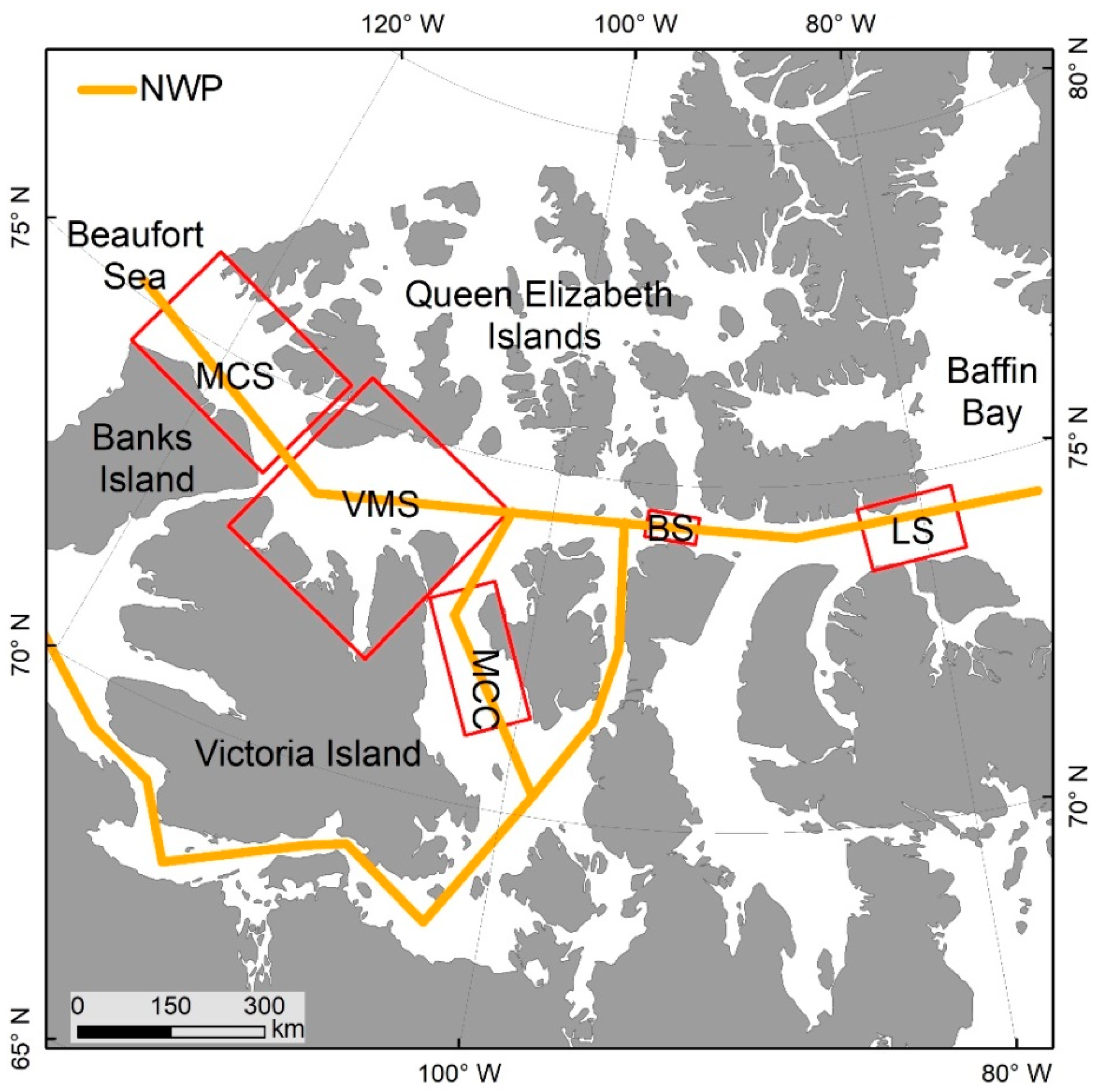
2. Study Area and Data

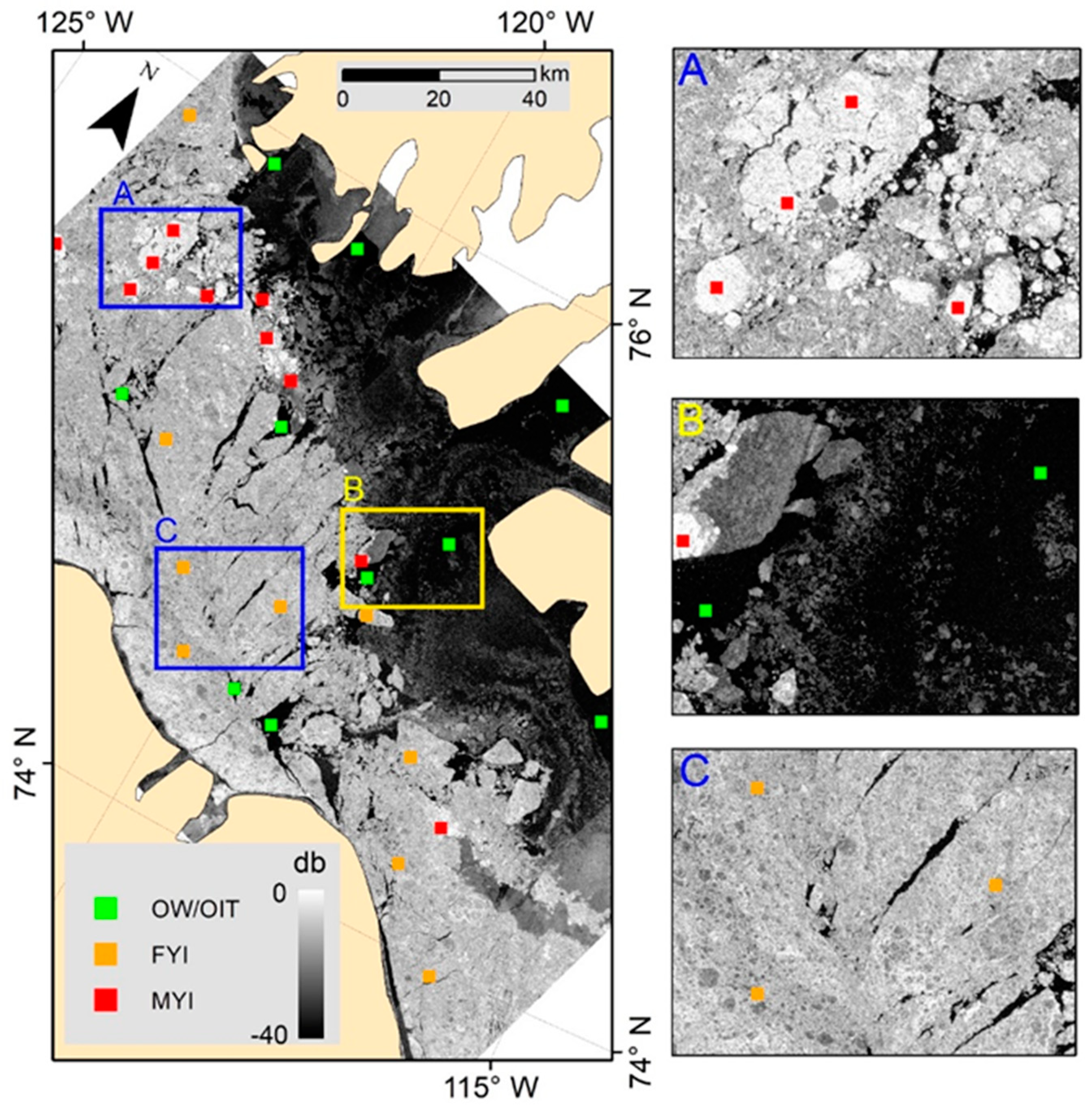
2.1. Study Area

The CAA is located at the north of the Canadian continental mainland. It is bounded by the Beaufort Sea to the west and the Baffin Bay to the east. CAA covers an area of around 1,500,000 km² and consists of 94 major islands and more than 36,000 minor ones. These islands are separated by numerous waterways, some major ones constitute the Northwest Passage. The passage is mainly covered by FYI and MYI all year round. However, owing to the recent significant changes in the Arctic climate, summer sea ice has decreased substantially [38], leading to an increasing number of vessels navigating through this once-impossible route. In our study, five critical water passages are selected, including M’Clintock Channel (MCC), Viscount Melville strait (VMS), M’clure Strait (MCS), Barrow Strait (BS), and Lancaster Sound (LS) (Figure 1).

2.2. Sentinel-1 A/B SAR Images

Sentinel-1A/B (https://sentinel.esa.int/web/sentinel/missions/sentinel-1) is a constellation of two satellites. They are developed and operated by the European Space Agency (ESA), carrying a SAR system that operates in the C-band dual-polarized channel. Sentinel-1 has four standard operational modes: Stripmap (SM); Interferometric Wide Swath (IW); Extra Wide Swath (EW); Wave (WV). In this study, we use the Level-1 Ground Range Detected (GRD) product. All scenes were acquired in EW Mode with dual polarization (HH and HV). This mode employs the Terrain Observation with Progressive Scans SAR (TOPSAR) technique to acquire data over a wider area using five sub-swaths, EW1-EW5 with lowest-highest incidence angle ranges, respectively. The swath width for EW Mode is approximately 400 km with an incidence angle ranging from 18.9° to 47° and pixel spacing of 40 m × 40 m. The constellation provides relatively large spatial coverage and high temporal resolution.

We selected 17 Sentinel-1 EW dual-polarized SAR images (HH and HV), acquired between September and March of 2016–2019 as shown in

Table 1. List of Sentinel-1 SAR images used for training and classification in NWP.

No.	SAR Images for Training				SAR Images for Classification
	Acquisition Date	Acquisition Time	Coverage	Satellite	Acquisition Date	Acquisition Time	Coverage	Satellite
1	11-03-2019	13:49:25	MCC	Sentinel-1A	16-01-2016	13:33:03	MCC	Sentinel-1A
2	10-12-2017	13:49:21	MCC	Sentinel-1A	21-04-2018	13:49:20	MCC	Sentinel-1A
3	07-01-2018	22:09:48	LS	Sentinel-1B	27-12-2017	12:18:05	LS	Sentinel-1A
4	05-02-2019	14:21:16	VMS	Sentinel-1B	26-11-2016	12:18:07	LS	Sentinel-1A
5	06-04-2019	14:21:16	VMS	Sentinel-1B	23-03-2017	14:21:03	VMS	Sentinel-1B
6	21-10-2018	13:23:53	BS	Sentinel-1B	24-02-2019	14:13:04	VMS	Sentinel-1B
7	22-09-2018	14:53:43	MCS	Sentinel-1B	30-09-2016	13:31:30	BS	Sentinel-1B
8	26-09-2018	14:21:19	MCS	Sentinel-1B	04-10-2018	14:53:44	MCS	Sentinel-1B
9	14-11-2017	14:53:37	MCS	Sentinel-1B

. Nine images acquired in different dates and covering different straits are used for training data, and eight images are used for MYI identification and sea ice classification. The images cover the five passages (listed in the previous sub-section) and are coded as shown in Table 1. All Sentinel-1A/B images were provided by the Alaska Satellite Facility.

2.3. Comparison Data

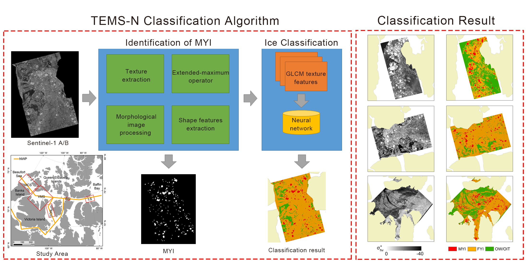
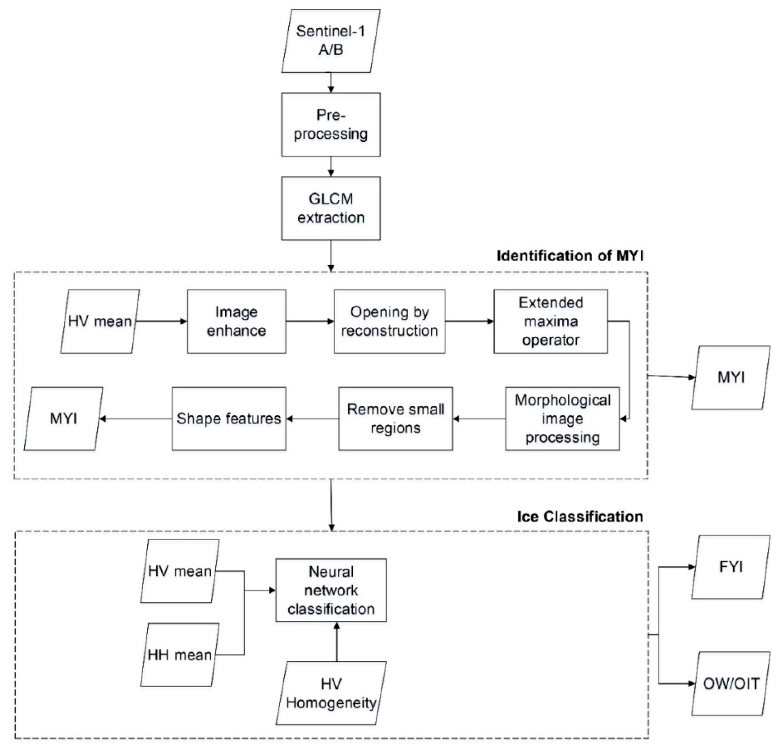
Three datasets were used to compare with the classification results in this study. The first is CIS ice charts (https://iceweb1.cis.ec.gc.ca/CISWebApps/page1.xhtml?lang=en). For the Arctic region, ice charts are generated at weekly basis using visual analysis of remote sensing data (mainly SAR) combined with meteorological and climatic information at a grid resolution of 5 km. In each chart the scene is divided into polygons (subjectively selected) and each polygon is assigned a code (called egg code), indicating the existing ice types (up to three types) and their concentrations based on the subjective estimate of the ice analysts. Details can be found in the manual of procedures for observing and reporting ice conditions [39].

The second dataset is MYI concentration maps from the Environment Canada’s Ice Concentration Extractor (ECICE) algorithm [40] with modifications to account for anomalous observations during transition seasons [41]. It uses a combination of scatterometer and microwave radiometer, then adds air temperature and sea ice drift data to correct for anomalies of the microwave observations. The algorithm outputs concentrations of ice types from each pixel. Maps of MYI concentrations were downloaded from University of Bremen (https://seaice.uni-bremen.de/multiyear-ice-concentration/data-access/) at grid spacing of 12.5 km. As the algorithm does not work during the melt season, the data record usually spans October to May.

The third dataset offers maps of FYI and MYI from an algorithm that also uses a combination of scatterometer and passive microwave observations at 4.45 km resolution [9]. Data are available from winter (November to April) seasons of 2002 throughout 2017.

Table 2. Comparison datasets.

Datasets	Data Source
CIS ice chart	SAR imagery (Radarsat/Envisat)
ECICE	scatterometer from ASCAT, brightness temperature from AMSR-2, Air temperature at 2 m level ERA-Interim and sea ice drift data
Zhang	microwave scatterometer data from QuikSCAT and the ASCAT, microwave radiometer data from the AMSR-E, SSMI/S, and AMSR-2

includes radar data (SAR and scatterometer) used in each set of comparison data.

3. Method

The study area hosts an ice cover composed of FYI, MYI, and open-water (OW)/other ice type (OIT). The OIT includes smooth fast ice, from which backscatter signature is typically low. OIT is difficult to be distinguished from smooth OW in SAR image. Therefore, we classify them as one type in this paper. As mentioned above, the new method presented here involves two parts (Figure 2). This method is referred to by the first letters of the five undermentioned processes: TEMS-N. The first part is about identification of individual MYI floes. It employs four processes: texture extraction, extended-maximum operator, morphological image processing and shape features extraction (TEMS). The second part is about classification of the rest of the scene into FYI and OW/OIT. It uses a neural network scheme (N) with input from three GLCM texture parameters: mean from ${\sigma }_{hv}^o$, mean from ${\sigma }_{hh}^o$ and homogeneity from ${\sigma }_{hv}^o$. Another method that uses texture parameters only in a neural network scheme (referred to as TPO) is used to compare its results against TEMS-N and therefore assess the extra processes involved in TEMS-N (besides texture) to identify individual MYI floes.

3.1. Pre-Processing

The pre-processing consists of thermal noise removal, radiometric calibration with conversion to dB and terrain correction, all performed in the Sentinel Application Platform (SNAP) which was developed by ESA (http://step.esa.int/main/toolboxes/snap/). SNAP provides a thermal noise removal function which uses a noise look-up table (LUT) provided by Sentinel-1 products. The LUT could be used to derive calibrated noise profiles. Calibration is carried out by using parameters within the Sentienl-1 product for radiometrically calibrated backscatter values (sigma 0), then the backscatter values are converted to dB using a logarithmic transformation. The terrain correction is applied to output data using Range Doppler Terrain Correction Operator in SNAP. The images should be corrected for these effects in the terrain correction step by using digital elevation model (ACE30 was used). Polar stereographic projection/WGS 84 was chosen for map coordinate system in terrain correction resulting in a geocoded image.

Variation of backscatter with respect to incidence angle is shown in Figure 3. No obvious decreasing trend with the angle is observed in the FYI or MYI data. On the other hand, both backscatter coefficients demonstrate strong angular decreasing trend for the OW/OIT category; −0.37 dB/deg for ${\sigma }_{hh}^o$ and −0.15 dB/deg for ${\sigma }_{hv}^o$. Based on these data, and given the difficulty of applying incidence angle correction to pixels of unknown ice types, we decided to proceed with the classification without incidence angle correction.

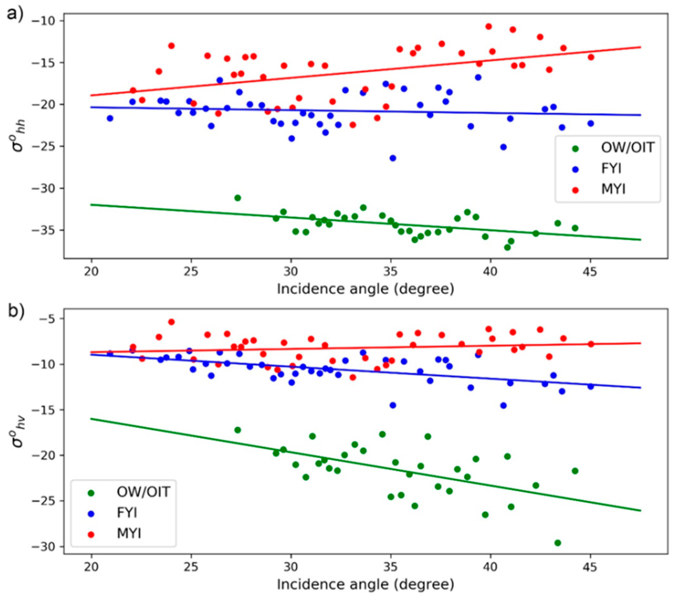
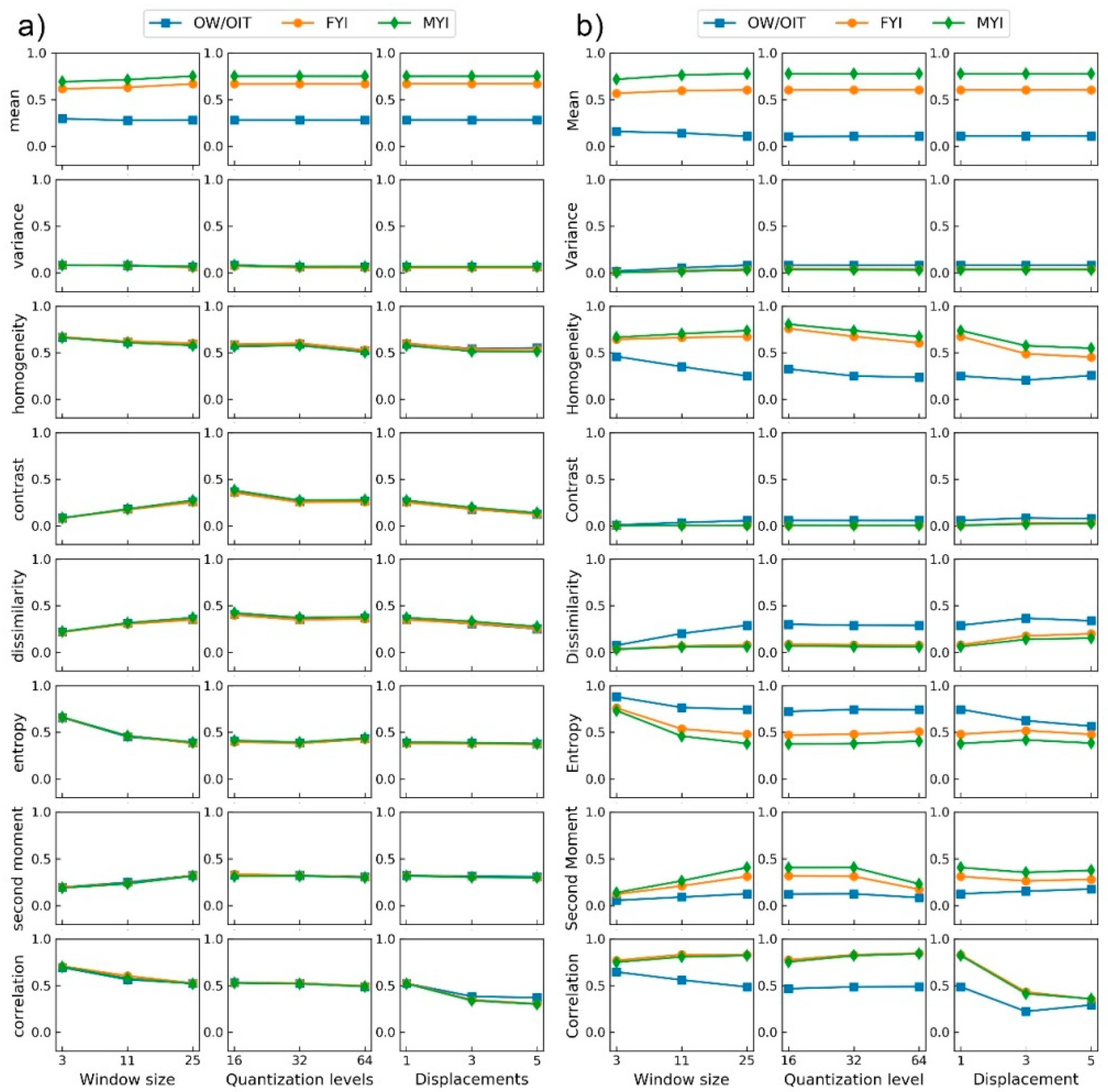
3.2. Texture Feature Selection

The GLCM parameters characterize the texture of objects in an image by calculating a set of grey-tone spatial-dependence matrices using various angular and distance relationships between neighboring pixel pairs; then extracting statistical measures from the matrices [28]. The window size (W), displacement (D), quantization level (K) and orientation are inputs for calculations of the matrices. Texture parameters derived from the GLCM are the mean, variance, homogeneity, contrast, dissimilarity, entropy, second moment and correlation [28,29].

Previous studies that used GLCM texture for ice classification usually set the K, W, D as fixed values. In this study, we tested the above-mentioned eight texture statistical parameters using different combinations of W (3, 11 and 25), D (1, 3 and 5) and K (16, 32 and 64) for their abilities to discriminate the given ice types. Nine images acquired in different months were used for this test. Samples from each ice type (OW/OIT, FYI and MYI) were selected using visual interpretation of the images. Figure 4 shows the samples from the ${\sigma }_{hv}^o$ SAR image acquired on 22 September 2018. The samples from SAR images for training (Table 1) are used to calculate the backscatter coefficient as a function of incidence angle (Section 3.1), evaluation of classification capability of each texture parameter and in the selection of most powerful texture features for training the neural network model (Section 3.5).

None of the texture parameters derived from the co-polarization backscatter ${\sigma }_{hh}^o$ is found to be useful for discriminating the three surface types (Figure 5a). Different selections of the W, D, and K have virtually no discrimination power. Only the mean from ${\sigma }_{hh}^o$ can discriminate between OW/OIT and two sea ice types (MYI and FYI). On the other hand, texture parameters derived from ${\sigma }_{hv}^o$ data have better discrimination power. Figure 5b shows the superiority of the mean in discriminating between OW/OIT and the two types using any combination of W, D, and K. However, discrimination between FYI and MYI is still relatively ambiguous. The variance and contrast obtained from ${\sigma }_{hv}^o$ data are particularly useless in discriminating any type using any combination of W, D, and K. Homogeneity and correlation had good performance in discriminating OW/OIT from other ice types. The performance improves with increasing window size and degrades with increasing displacement. Nevertheless, these results suggest that discrimination between FYI and MYI is still difficult using texture alone.

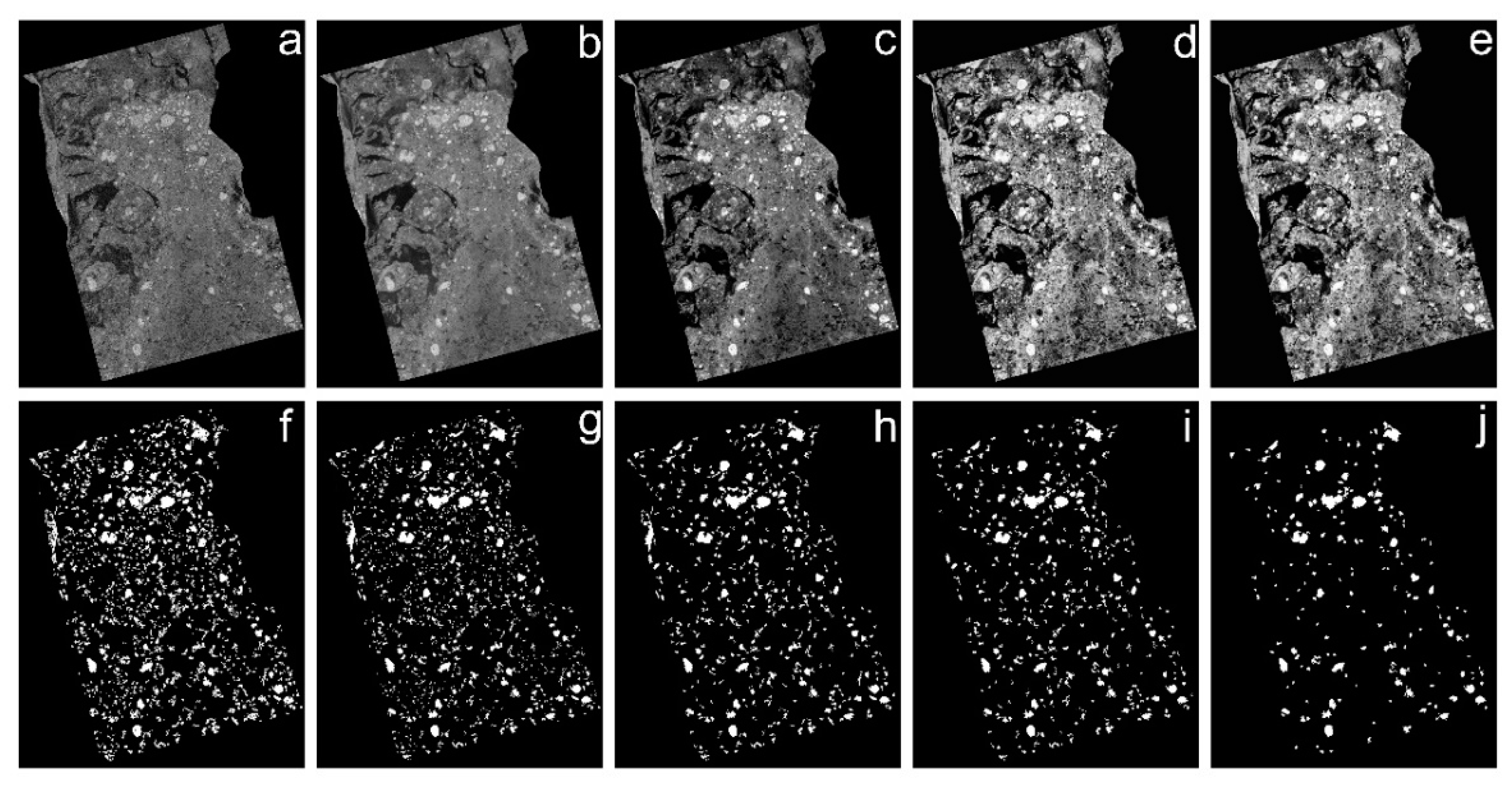
3.3. The TEMS Method

The synthesis of the TEMS-N method is presented in Figure 2. Here, the six steps for identifying MYI floes in the TEMS component of the algorithm are presented. The neural network component is present in a later section. It should be noted that TEMS identify MYI floes based on their rounded/elliptic shape and high backscatter/texture. This criterion applies to most MYI floes as explained in Section 5. Results from each step are presented in Figure 6 for the image of a section in the Beaufort Sea acquired on 30 September 2016. The original SAR image, discretized into 256 levels, is shown in Figure 6a, where MYI floes appear bright against the background. The image of GLCM texture mean parameter from ${\sigma }_{hv}^o$ with (W = 11, D = 1, K = 32) is shown in Figure 6b. Here, contrast between the MYI floes and background is enhanced.

The first step involves enhancement of ${\sigma }_{hv}^o$ image using a linear stretch of the 20–80% range of grey tone to occupy the full scale (0–256) (Figure 6c). This step removes the darkest area (e.g., OW and smooth fast ice) and accentuates the MYI floes with uneven brightness. It is followed by the adaptive histogram equalization to improve the image contrast (Figure 6d) which further enhances the appearance of some MYI floes against the dark background.

The second step, opening-by-construction, is an erosion followed by a morphological reconstruction [42]. It was performed to eliminate small objects that are considered to be noise (Figure 6e), hence facilitate extraction of MYI later. The erosion “shrinks” an image according to the shape of a given structuring element, removing objects that are smaller than the given element. We used the structuring element with 8 × 8 pixels in this step. The dilation step “regrows” the remaining objects by the same shape.

In the third step, the extended-maxima operator is applied to identify bright objects (potentially MYI and rough FYI). The output is a binary image (Figure 6f). The extended-maxima operator is composed of two steps, H-maxima transform and regional maximum [43]. The H-maxima transform, where h is a nonnegative scalar, suppresses all maxima in the intensity image whose height (grey tone) is less than h, as shown in the following:

$${\mathrm{H}\mathrm{MAX}}_h\left(f\right)={\mathrm{R}}_f^{\delta }\left(f-h\right)$$

(1)

where f is the greyscale of original greyscale image, and h is the threshold value. We set h at a value of 50. The extended-maxima EMAX are as shown in the following:

$${\mathrm{E}\mathrm{MAX}}_h\left(f\right)=RMAX\left[{\mathrm{MAX}}_h\left(f\right)\right]$$

(2)

The regional maxima connect pixels with a constant intensity value and whose pixels outside the region’s boundary have a lower value. By using the extended-maxima operator, we identify areas with higher grey tone intensity in SAR images (potential MYI floes). The drawback is that some MYI floes may include some dark areas that would be rejected by the extended-maximum operator. This may lead to misidentification of ridges, rubble, rims, and surface deformation as MYI. The following steps are implemented to mitigate these problems.

In the fourth step, the morphological image processing is used to improve the identification of MYI floes (Figure 6g). It includes morphological closing, eroding, and filling holes. Closing is a dilation followed by an erosion. We used the structuring element with 5 × 5 pixels for closing and eroding in this step. Closing and eroding can remove some small ridges and some connection between the ice floes. Filling holes can fill some dark area in the MYI floes.

In the fifth step the objects with area less than 1000 pixels (i.e., small areas) are removed (Figure 6h). This was performed to save processing time in the next (and last) step of “shape features” that appears in the flowchart in Figure 2. The MYI ice floes has more rounded edges than younger ice types which are caused by the more frequent collision of floating floes [44]. This information is used in the sixth step.

The sixth step is about quantifying some features that qualify the surviving regions as being MYI floes. It simply keeps bright objects with round shape and reject those with linear or non-defined shapes (i.e., ridges and deformed ice). Three features were used: eccentricity, area, and extent. The first feature is the eccentricity of the ellipse that has the same second-moments as the object. It is the ratio of the distance between the foci of the ellipse and its major axis length. The value is between 0 and 1. An ellipse whose eccentricity is 0 is a circle, while an ellipse with eccentricity of 1 is a line segment. We used this feature to remove some deformed FYI objects with high backscatter similar to that of MYI but assume a long linear shape. Area is defined as the actual number of pixels in the object to be labeled. Extent is the ratio of number of pixels inside the region to pixels in the total bounding box around the region. A threshold of the eccentricity is set to 0.95. If the eccentricity is greater than this threshold, the region is not considered to be MYI floe. The result is shown in Figure 6i (a long linear shape in the upper left corner of the image is removed). If the area is less than 5000 pixels and the extent is less than 0.5, the region will be removed. This step removes ridges with high backscatter. The final result in shown in Figure 6j.

After identifying MYI floes, we used the neural network model to classify the rest of the image into FYI or OW/OIT types. Three GLCM texture features were selected as input: Mean (W = 11, D = 1, K = 32) and Homogeneity (W = 25, D = 1, K = 32) from ${\sigma }_{hv}^o$ data and mean (W = 11, D = 1, K = 32) from ${\sigma }_{hh}^o$.

3.4. The TPO Method

Although Figure 5 demonstrates the difficulty of using GLCM only to classify FYI and MYI, the TPO method is used to classify these two surfaces in addition to the OIT in order to demonstrate the advantage of employing the above-mentioned steps in the TEMS-N method. For this task, we selected the following texture features: Mean (W = 11, D = 1, K = 32), Homogeneity (W = 25, D = 1, K = 32), Entropy (W = 25, D = 1, K = 32), Second Moment (W = 25, D = 1, K = 16) (all from ${\sigma }_{hv}^o$ data) and mean (W = 11, D = 1, K = 32) from ${\sigma }_{hh}^o$. Then the five texture features were put into the neural network scheme.

3.5. Neural Network Classification Algorithm

The neural network is a computation model whose layered structure resembles the networked structure of neurons in the brain, with layers of connected nodes [45]. Many studies have demonstrated the usefulness of this model in sea ice classification [46,47,48,49]. We used single-layer feedforward networks model in MATLAB (The MathWorks, Inc., Natick, MA, USA). The chosen network training function updates weight and bias values according to Levenberg-Marquardt optimization. This function is often the fastest backpropagation algorithm in the toolbox of MATLAB. The hidden layer size is 10. The normalization step is applied to both the input vectors and the target vectors in the dataset. The training images are shown in Table 1. The images for classification were not used in training. For the TEMS-N method, there are two and three neurons in the input and output layer, respectively. For the TPO method, the input layer has five input neurons from GLCM features and the output layer has three neurons. The training data are composed by GLCM features values of three sea ice types, which are input into model for training after normalization.

3.6. Validation Method

Visual classification of ice types in SAR images was used to evaluate results from TEMS-N and TPO methods. This was performed using one image every month from March to September. Decision on ice types from selected points was compared with TPO and TEMS-N results from the same point. Stratified random sampling is employed to derive the sampling points, which is a commonly used sampling technique in the accuracy assessment of land cover maps [50,51]. It satisfies the basic accuracy assessment objective and most of the desirable design criteria. It can also increase the sample size in classes occupying areas to reduce the standard errors of the class-specific accuracy estimates for these rare classes. The user’s accuracy, product’s accuracy, kappa coefficient and overall accuracy were calculated from confusion matrices (shown in Section 4.2) as tools of assessment. Finally, classification maps from TEMS-N are compared with operational ice charts and ice type estimates from two microwave radiometer and scatterometer-based algorithms in order to compare ice type mapping in coarse-resolution products against SAR fine-resolution results.

4. Results

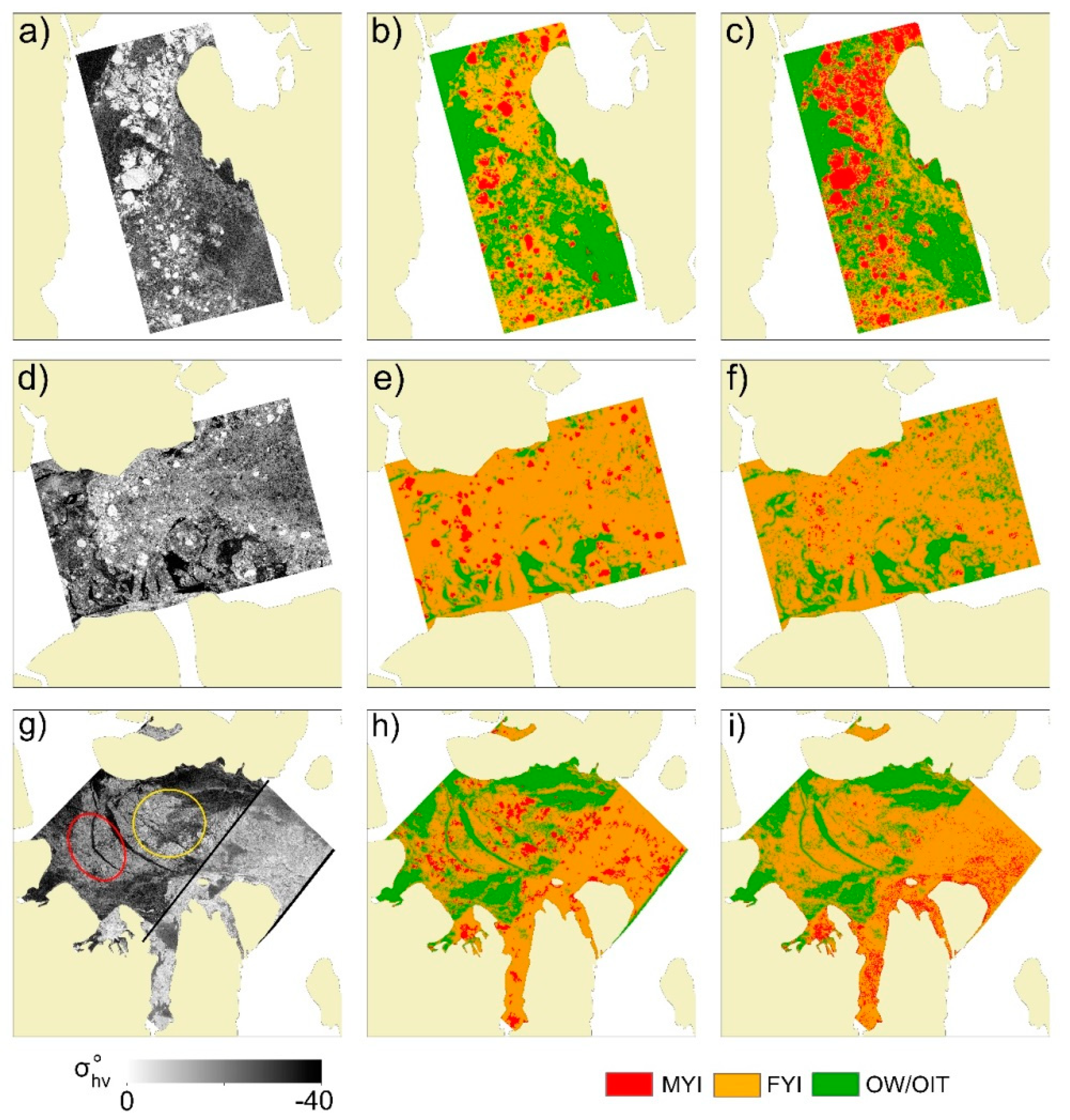
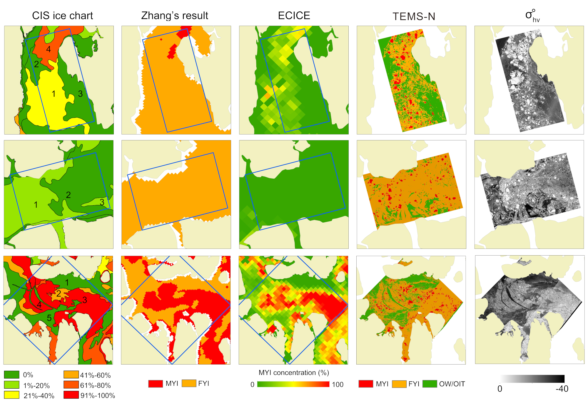
4.1. Qualitative Comparison of Classification Maps against SAR Images

In this section, we present comparison of classification maps from using TEMS-N and TPO methods against selected ${\sigma }_{hv}^o$ images from dates and areas listed in Table 1. Visual interpretation of the images is used for the comparison.

The top image in Figure 7, acquired on 16 January 2016, shows a section in the M’Clintock Channel. This channel is a pathway of sea ice from the central Arctic, but it does not end at an open sea. Therefore, numerous MYI floes usually accumulate in the channel (appear as bright rounded objects in the ${\sigma }_{hv}^o$ images). The figure shows that TEMS-N method identifies most of the visible MYI floes in the ${\sigma }_{hv}^o$ image and avoids misidentification of the relatively high backscatter from deformed FYI as being MYI. On the other hand, the TPO method overestimates the areal extent of the MYI because the texture of the surrounding FYI is very similar to that of MYI. TEMS-N and TPO methods have similar classification results of OW/OIT. Similar classification performance of the two methods was observed in the other image of M’Clintock Channel acquired on 21 April 2018 (not shown here).

The middle image in Figure 7 is from Lancaster Sound at a location near its eastern end where it connects to the Baffin Bay. The image was acquired during late fall (26 November 2016). The freeze-up at this location usually starts during the first week of October though it may be delayed by a month because of strong wind and tidal activity. Moreover, ice consolidation rarely prevails in this location [52]. MYI floes appear bright with identifiable rounded shape in the ${\sigma }_{hv}^o$ image. The surrounding deformed FYI appears in different grey shades. Dark areas could be smooth FYI or OIT. The TEMS-N method seems to reproduce the individual MYI floes while the TPO method reproduces a fewer number of floes. Similar TEMS-N performance was found in the scene of 27 December 2017 in the Lancaster Sound though the TPO method reproduces more floes. The good contrast between MYI floes and the background in both images of the Lancaster Sound allows the extended-maxima function to identify the MYI floes easily. The separation of the floes and their fairly well rounded shape justify the use of morphology processing and shape features. The TPO method could not classify MYI effectively in both images.

The bottom scene shows a scene located in the Viscount Melville Sound, acquired on 23 March 2017. This location is a choke point on the western part of the Northwest Passage where old ice concentration was observed to be relatively high in the 2000′s (~40%), up from 30–50% in the 1970′s [53]. Nevertheless, the ${\sigma }_{hv}^o$ image reveals only a few MYI floes with small size. The thermal noise is apparent in this scene and is replicated in the results from both methods. Both methods misclassified OW/OIT as FYI in the areas with thermal noise. The TEMS-N method identifies MYI floes in this scene though more floes are identified than what is already visible in the ${\sigma }_{hv}^o$ images. This is apparent in the areas marked by the red ellipse and yellow circle (the latter is enlarged in Figure 8). The well-identified rounded MYI floe is reproduced in the TEMS-N image. However, other MYI floes in TEMS-N map originate from bright areas which may not form circular shapes in the original ${\sigma }_{hv}^o$ image. The uneven distribution of backscatter, hence texture, from MYI or deformed FYI adds to the complication of MYI floe identification. The FYI (grey areas in the ${\sigma }_{hv}^o$ images) is fairly well identified by TPO method in the scene of 23 March 2017 but misidentified as MYI in the scene of 24 February 2019 in the Viscount Melville Sound and 4 October 2018 over the M’clure Strait (not shown here) because it has high backscatter and texture, both similar to the MYI.

4.2. Accuracy of the Classification Schemes

Confusion matrices were calculated to summarize the accuracy of the two classification methods against the visual classification. Results are presented in

Table 3. Classification results from the TPO method.

No.	Coverage	Date	User’s Accuracy (%)			Producer’s Accuracy (%)			Kappa	Overall Accuracy (%)
			OW/OIT	FYI	MYI	OW/OIT	FYI	MYI
1	MCC	16-01-2016	92.93%	97.82%	78.36%	99.20%	80.30%	97.81%	0.8659	91.59%
2	MCC	21-04-2018	99.54%	69.25%	79.78%	59.23%	75.39%	98.88%	0.6809	79.06%
3	LS	27-12-2017	100.00%	88.77%	77.69%	77.34%	94.64%	72.22%	0.7413	87.29%
4	LS	26-11-2016	97.60%	90.44%	97.80%	100%	98.84%	62.24%	0.8569	92.71%
5	VMS	23-03-2017	100.00%	86.13%	91.00%	90.04%	98.03%	65.47%	0.8290	90.31%
6	VMS	24-02-2019	100.00%	92.08%	19.39%	91.19%	42.20%	98.29%	0.4264	59.75%
7	BS	30-09-2016	99.63%	54.49%	89.00%	68.29%	100%	48.11%	0.5908	73.33%
8	MCS	04-10-2018	99.69%	99.63%	12.30%	99.69%	28.84%	100.00%	0.3565	50.73%
		Overall	98.19%	83.69%	47.60%	84.58%	69.37%	81.53%	0.6191	75.81%

(for TPO method) and

Table 4. Classification results from the TEMS-N method.

No.	Coverage	Date	User’s Accuracy (%)			Producer’s Accuracy (%)			Kappa	Overall Accuracy (%)
			OW/OIT	FYI	MYI	OW/OIT	FYI	MYI
1	MCC	16-01-2016	98.75%	83.65%	95.00%	98.75%	97.44%	65.52%	0.8679	91.73%
2	MCC	21-04-2018	100.00%	90.41%	98.00%	86.98%	99.64%	76.56%	0.8696	93.27%
3	LS	27-12-2017	98.92%	97.48%	84.85%	97.87%	97.87%	83.17%	0.8931	96.30%
4	LS	26-11-2016	100.00%	99.71%	86.87%	100.00%	98.12%	97.73%	0.9553	98.31%
5	VMS	23-03-2017	95.20%	91.74%	83.00%	91.54%	94.07%	81.37%	0.8532	91.73%
6	VMS	24-02-2019	100.00%	97.89%	52.00%	97.73%	90.61%	92.86%	0.8715	93.02%
7	BS	30-09-2016	100.00%	78.76%	94.06%	74.28%	98.45%	80.51%	0.7749	86.66%
8	MCS	04-10-2018	100.00%	100.00%	49.00%	95.61%	92.95%	100.00%	0.8752	94.00%
		Overall	98.97%	93.48%	80.35%	91.51%	96.17%	81.58%	0.8715	93.26%

for (TEMS-N method). The average overall classification accuracy from the eight scenes are 75.81% for the TPO method and 93.26% for the TEMS-N method. The overall user’s and producer’s accuracy are highest for the OW/OIT class and lowest for the MYI class, with the producer’s accuracy always higher. The overall user’s accuracy of all classes from the TEMS-N classification are higher than the TPO classification (e.g., for MYI it is 80.35% and 47.60% from TEMS-N and TPO, respectively). The overall producer’s accuracy is also higher from TEMS-N. The TPO method often overestimate MYI areas.

The kappa coefficient is a statistical measure of agreement between two raster images (in this study, they are the result from the classification methods and the manual classification) [54]. Kappa ranges from 0 to 1, with 1 means perfect agreement and 0 means agreement equivalent to chance. It scores overall values (i.e., from all scenes) of 0.6191 and 0.8715 from TPO and TEMS-N, respectively.

Data from individual scenes (Table 3 and Table 4) show that TEMS-N method has higher kappa and overall accuracy than TPO method from all tested scenes. The lowest kappa from TEMS-N is 0.7749 estimated from the 30 September 2016 image. In this image, the misclassification of OW/OIT as FYI caused low producer’s accuracy of OW/OIT and low user’s accuracy of FYI. The errors of OW/OIT in this image are mainly caused by thermal noise. The lowest kappa from TPO is 0.3565, obtained from the 4 October 2018 image. TPO classified many FYI ice floes with high brightness as MYI in the 4 October 2018 image. This caused low producer’ accuracy of FYI and low user’s accuracy of FYI. The TEMS-N method demonstrates better performance of identifying MYI compared with the TPO method. Two images located in the MCS and VMS (acquired on 24 February 2019) have lower user’s accuracy of MYI from the two methods, with the lowest value from the TPO method. Many FYI pixels were misclassified as MYI by the TPO method in other images, which caused low user’s accuracy of MYI. Most of images have high user’s and producer’s accuracy of OW/OIT by both methods. FYI classification errors is caused mostly by the similarity of texture features between FYI and MYI.

4.3. Comparison against Other MYI Classification Data

Three datasets of ice type/concentration maps (all from coarse-resolution sources) have been used for comparison against the output from TEMS-N method. These are the CIS weekly ice charts (concentration of MYI), MYI concentration maps from ECICE algorithm produced by Bremen University and maps of Arctic sea ice classification (FYI and MYI) produced a published study [9]. The latter is referred to as ZR (Zhang’s results). The three products are described in Section 2.3. Examples of comparison from the four methods, along with the original ${\sigma }_{hv}^o$ images, are shown in Figure 9. The figures aim at assessing the results from the coarse-resolution sources against the fine-resolution TEMS-N results.

In the CIS charts in Figure 9 each polygon is assigned MYI concentration (including second-year and older ice). The ZR product assigns one ice type, MYI or FYI, to each pixel of 4.45 km. The ECICE product uses a combination of passive and active microwave observations (same as the ZR method) and provides the concentration of MYI at grid spacing of 12.5 km. It should be noted that the resolution of the TEMS-N results from Sentinel-1 is much finer than the resolution of all the comparison datasets.

Table 5. Comparisons among the CIS chart, ECICE and the TEMS-N result in regions in some scenes.

Coverage	Date	Polygon	CIS		TEMS-N			ECICE
		No.	FYI	MYI	OW/OIT	FYI	MYI	MYI
MCC	16-01-2016	1	60%	40%	36.70%	53.27%	10.03%	19.59%
		2	100%	-	92.56%	7.42%	0.01%	7.45%
		3	100%	-	70.57%	28.04%	1.39%	5.29%
		4	20%	80%	17.07%	65.77%	17.16%	39.88%
LS	26-11-2016	1	90%	10%	1.32%	80.54%	6.56%	1.32%
		2	100%	-	0.00%	84.58%	3.95%	0.00%
		3	90%	10%	0.00%	87.94%	7.53%	0.00%
VMS	23-03-2017	1	100%	-	63.74%	35.46%	0.80%	15.61%
		2	50%	50%	6.75%	78.45%	14.80%	57.50%
		3	10%	90%	37.56%	57.37%	5.07%	83.36%
		4	10%	90%	17.14%	72.52%	10.35%	69.31%
		5	100%	-	61.42%	36.96%	1.62%	29.34%

includes quantitative comparison of ice type concentration from TEMS-N versus CIS and ECICE. The digital values of the concentrations are not available from the ZR.

In the top scene of the MCC site (Figure 9), acquired on 11 January 2016, maps of MYI from CIS, ZR and ECICE reproduce nearly same concentration observed in the fine-resolution TEMS-N (particularly in polygon 4). The only exception is the failure of ZR to reproduce the concentration that appears in the lower part of the image (polygon 1). From Table 5, polygons 1 in the CIS map of this scene show 40% MYI concentration while TEMS-N show 10%. These are not the best polygons for comparison because part of the polygon extends outside the SAR frame. Please note that the 0% MYI concentration in polygons 2 and 3 is reproduced in TEMS-N data and to some extent in ECICE data. In the scene of 21 April 2018 over M’Clintock Channel, the difference between MYI concentration from TEMS-N and both CIS and ECICE is large possibly because of the large difference between the spatial resolution of the two data sets.

In the middle scene in Figure 9 (26 November 2016) the 10% MYI concentration in polygon 1 matches an area where several MYI floes in TEMS-N is observed while the 0% MYI concentration in polygon 2 ignores a few visible floes. Once again, the advantage of producing maps at the better spatial resolution of SAR is evident. In this image, the concentrations of MYI and FYI from TEMS-N are not significantly different from those obtained from the other three datasets. In the 27 December 2017 image MYI concentration from CIS also agree with TEMS-N while ECICE overestimates it.

In the bottom scene of the VMS (Figure 9), a few MYI floes appear as bright spots in the ${\sigma }_{hv}^o$ image and are replicated in the TEMS-N results. However, a larger and continuous MYI cover is shown in the three coarse-resolution comparison maps. Based on visual interpretation of SAR image and the TEMS-N results, all three methods identified areas between the visible MYI floes as MYI. These areas usually contain deformed FYI if the ice regime is highly mobile, which is the case in the western Arctic region. More discussions of the physical reason are presented in Section 5. It is interesting to note that the CIS map in the bottom panel of Figure 6 captures the leads in polygon 4, which is visible in the original ${\sigma }_{hv}^o$. This is an advantage of the visual analysis when the polygon is narrowed down to capture a single feature in the SAR image. The apparent FYI in polygon 1 and 5 are correctly classified in all other maps.

The striking quantitative information from the 23 March 2017 data in Table 5 is the significantly lower MYI concentration in polygons 3 and 4 from TEMS-N (5% and 10.3%, respectively) compared to 90% from the CIS chart and average of 75% from ECICE. Although estimates of ice types and concentrations in operational ice charts are usually conservative (see next section), it is also possible that TEMS-N underestimates the MYI concentration in this scene because of thermal noise.

5. Discussion

Operational ice charts are generated to identify sea ice types and their partial concentrations in delineated areas (called polygons) generated manually by trained ice analysts. The information is used by marine operators to support navigation decisions particularly regarding avoidance of hazardous ice such as MYI. With the assumption of uniform distribution of concentration of each ice type inside the polygon, identification of individual MYI floes (the hazardous objects) is missing in the ice charts. This information, however, is available in the fine-resolution SAR images and, in fact, is retrieved through the visual analysis of the images. Although many research studies were performed to automate this retrieval, an automated detection method is still far from achieving the robustness required by an operational scheme. This study is an attempt to develop an automated tool to identify MYI floes in SAR images, then classify the rest of the scene.

Prior methods of using texture to detect MYI are disadvantaged by the intensive computations required to generate the texture parameters and the non-inclusive classification results due to overlapping texture values from different ice types. This problem is more severe in the present data set than what has been reported in previous studies [25,48,55] because we found no texture parameter can discriminate between MYI and FYI.

The challenge of identifying MYI cover using radar imagery data is the heavy overlap between the MYI backscatter (and texture) and the deformed FYI in the surrounding. The deformed ice results from the mobility of the ice cover, especially in the presence of MYI floes, which is usually intensive in the western section of the Arctic due to the Beaufort Sea Gyre [56]. Due to the coarse resolution of the comparison data used in the present study, particularly the operational ice mapping product, the deformed ice is usually considered part of the MYI cover. Physically speaking, the deformed ice between MYI floes is likely to be seasonal ice, not MYI. This is because during the melt season (which MYI floes survive) all surface roughness/deformation forms, including protruding upturned ice blocks, usually melt, leaving the MYI floes with smooth undulating surface, which features hummocks and flat depressions (i.e., frozen melt pond). The floe shape is typically rounded or elliptic, i.e., not angular or elongated. This assumption is used in the present method. Although it is well-recognized and usually true because of the continuous collision of the floes with the surrounding ice during its long life, any deviation from this typical shape presents a limitation on the application of the present method.

TEMS-N method combines texture with extended-maximum operator, morphological, and shape features to identify individual MYI floes. Subsequently, a neural network scheme, trained by a few texture parameters is applied to perform the classification. A few advantages of the steps involved in TEMS-N are demonstrated in this paper. The extended-maxima operator can extract areas with higher intensity in SAR images (potential MYI floes) to adapt the change of backscatter of MYI with days and seasons. When the backscatter or its texture varies inside the same MYI floe, the morphology operator in TEMS-N can resolve the identification of the whole floe by filling “holes” inside the floe. In high latitude areas, such as M’clure Strait and Viscount Melville strait, deformed FYI returns high backscatter and texture similar to that of MYI, using texture parameters alone in a classification scheme lead to misidentification as MYI. The shape features, including eccentricity, area, and extent, could remove misidentification of deformed FYI or ridges.

Although TEMS-N has improved the identification of MYI floes, the deformed FYI could still complicate the classification result. It is difficult to ensure the accuracy in the presence of extensive and heavy deformed ice cover. This is evident in the three images in VMS and MCS, which typically have high concentration mixtures of deformed, thick FYI and MYI. This leads to low MYI user’s accuracies as shown in Table 3 and Table 4. Classification results are also affected by thermal noise, an inherent feature in Sentinel-1 images. In this study, thermal noise removal is performed based on the given information. However, the remaining thermal noise still leads to misclassification of OW/OIT as FYI. Although methods for thermal noise removal was developed (e.g., [57]), there is still no simple and effective method to remove the noise completely. A better thermal noise removal approach could improve the classification.

Operational ice charts usually provide conservative information, tending to overstress thicker and older ice types such as MYI [58]. This is favored by operational community. They provide gross information about ice type composition and their partial concentration within identified polygons but details about the number, location, and size of hazardous ice floes are sometimes become critically needed. Comparison of results from TEMS-N method against CIS ice charts serves to shed light on this issue. An example is shown in the case of the VMS images (Figure 9 and Table 5). Here, the gross MYI concentration from CIS charts reveals 100% or near 100% in the shown polygons. The corresponding concentration of the identified floes from TEMS-N reveals only a range from 5% to 12%. Field observations or just airborne photos are still needed to reveal the true composition. Nevertheless, the present study demonstrates the advantage of the detailed information output from an automated SAR-based approach compared to the coarse-resolution operational maps based on subjective analysis of SAR images within large polygons. Information provided by TEMS-N method is needed for tactical navigation purposes when a ship sails in a hazardous ice field. So far, in this situation timely SAR images are provided to the ship to be analyzed by an expert onboard.

The conservative estimates of MYI concentration in the CIS charts are sometimes backed by estimates from ECICE algorithm as shown in a few cases such as the MCC scene of 16 January 2016, the VMS scene of 23 March 2017 (both shown in Figure 9) and MCS scene of 30 September 2016 (not shown). MYI concentration from the CIS charts is found to be identical to the results from TEMS-N in most cases. An example is found in two scenes of LS. The accuracy of CIS operational charts is demonstrated also in capturing the leads which are visible in the original ${\sigma }_{hv}^o$ image in the VMS scene of 23 March 2017 (Figure 9). This is an advantage of the visual analysis of SAR images when polygons are narrowed down to focus on a single/uniform ice type.

Results from this study demonstrate potential application of the method to reveal distribution of hazardous MYI floes in the route of an operational marine activity (e.g., ship navigation). This can offer a special product when it is crucially needed. In this study, we just selected SAR images from September to March of following year to avoid the summer season when the difference between FYI and MYI in SAR images diminishes and neither backscatter nor texture becomes useful for classification. However, ships often plan to navigate the Arctic waters through summer. Therefore, the sea ice classification, particularly MYI, from SAR in the melt season should be a focus of future studies. Although we just selected eight scenes for application in this paper, much more validation is needed.

6. Conclusions

In this study, we propose an automatic sea ice classification approach (TEMS-N) to identify individual MYI floes in SAR image and then classify the rest of the image through a neural network approach trained by a few texture parameters. The first part of the method employs texture, an extended-maxima operator, morphological, and shape features. The method has been applied to eight scenes of Sentinel-1 SAR images with pixel spacing of 40 m in a study area that includes a few passages within the CAA. This region needs detailed monitoring of MYI floes as they constitute hazard for marine operations through parts of the Northwest Passage. The selected SAR images cover the period from September to March of 2016 to 2019.

Results from TEMS-N classification compare favorably with visual analysis of Sentinel-1 SAR images. Comparison of classification results from TEMS-N and another classification scheme that uses texture parameters only (referred to as TPO) shows that adding morphological and geometrical processing in the former improves the classification accuracy (particularly MYI identification) significantly. TEMS-N achieves higher overall kappa coefficient (0.87) from all ice types compared to 0.25 from the latter. This shows TEMS-N has better agreement with manual visual classification than TPO. The overall MYI user’s and product’s accuracy from the TEMS-N method were 80.35% and 81.58%, respectively, while the TPO method accuracies are 47.60% and 81.53%. The overall FYI user’s and product’s accuracy from TEMS-N method were 93.48% and 96.17% which were higher than TPO method. The TEMS-N and TPO methods have similar and relatively low OW/OIT classification accuracy since the effect of thermal noise is more obvious for OW/OIT.

TEMS-N ice classification results were compared qualitatively and quantitatively against MYI concentration from the weekly ice charts of the CIS, an ice type concentration and ice type product from coarse microwave observations. The three sources are generated at a much coarser spatial resolution than SAR. Comparison has shown that identification of individual MYI floes by TEMS-N produce MYI concentration remarkably less than what is shown in the coarse-resolution products in most of the eight cases studied. Nevertheless, good agreement is found in a few cases.

In conclusion, the TEMS-N method is proven to be an effective method to classify sea ice and identify MYI floes using dual-polarized Sentinel-1 imagery. Future studies are needed to be focus on the thermal noise removal of image and sea ice classification, particularly MYI, in the melt season.

References

1. Maslanik, J.; Stroeve, J.; Fowler, C.; Emery, W. Distribution and trends in Arctic sea ice age through spring 2011. Geophys. Res. Lett. 2011, 38, L13502. [Google Scholar] [CrossRef]
2. Cavalieri, D.J.; Parkinson, C.L. Arctic sea ice variability and trends, 1979–2010. Cryosphere 2012, 6, 881–889. [Google Scholar] [CrossRef] [Green Version]
3. Polyakov, I.V.; Walsh, J.E.; Kwok, R. Recent changes of Arctic multiyear sea ice coverage and the likely causes. Bull. Am. Meteorol. Soc. 2012, 93, 145–151. [Google Scholar] [CrossRef]
4. Khon, V.C.; Mokhov, I.I.; Latif, M.; Semenov, V.A.; Park, W. Perspectives of Northern Sea Route and Northwest Passage in the twenty-first century. Clim. Chang. 2009, 100, 757–768. [Google Scholar] [CrossRef]
5. Smith, L.C.; Stephenson, S.R. New Trans-Arctic shipping routes navigable by midcentury. Proc. Natl. Acad. Sci. USA 2013, 110, 1191–1195. [Google Scholar] [CrossRef] [Green Version]
6. McLaren, A.S.; Wadhams, P.; Weintraub, R. The sea ice topography of M’Clure Strait in winter and summer of 1960 from submarine profiles. Arctic 1984, 37, 110–120. [Google Scholar] [CrossRef] [Green Version]
7. Melling, H. Sea ice of the northern Canadian Arctic Archipelago. J. Geophys. Res. Ocean. 2002, 107, 2-1–2-21. [Google Scholar] [CrossRef]
8. Howell, S.E.L.; Tivy, A.; Yackel, J.J.; McCourt, S. Multi-year sea-ice conditions in the western Canadian arctic archipelago region of the northwest passage: 1968–2006. Atmos. Ocean 2008, 46, 229–242. [Google Scholar] [CrossRef]
9. Zhang, Z.; Yu, Y.; Li, X.; Hui, F.; Cheng, X.; Chen, Z. Arctic Sea Ice Classification Using Microwave Scatterometer and Radiometer Data During 2002–2017. IEEE Trans. Geosci. Remote Sens. 2019, 57, 5319–5328. [Google Scholar] [CrossRef]
10. Maslanik, J.A.; Fowler, C.; Stroeve, J.; Drobot, S.; Zwally, J.; Yi, D.; Emery, W. A younger, thinner Arctic ice cover: Increased potential for rapid, extensive sea-ice loss. Geophys. Res. Lett. 2007, 34, 497–507. [Google Scholar] [CrossRef] [Green Version]
11. Kwok, R. Arctic sea ice thickness, volume, and multiyear ice coverage: Losses and coupled variability (1958–2018). Environ. Res. Lett. 2018, 13, 105005. [Google Scholar] [CrossRef]
12. Howell, S.E.L.; Duguay, C.R.; Markus, T. Sea ice conditions and melt season duration variability within the Canadian Arctic Archipelago: 1979–2008. Geophys. Res. Lett. 2009, 36. [Google Scholar] [CrossRef]
13. Howell, S.E.L.; Wohlleben, T.; Dabboor, M.; Derksen, C.; Komarov, A.; Pizzolato, L. Recent changes in the exchange of sea ice between the Arctic Ocean and the Canadian Arctic Archipelago. J. Geophys. Res. Ocean. 2013, 118, 3595–3607. [Google Scholar] [CrossRef]
14. Curlander, J.C.; McDonough, R.N. Synthetic Aperture Radar; John Wiley and Sons: New York, NY, USA, 1991; Volume 396. [Google Scholar]
15. Liu, H.; Guo, H.; Zhang, L. SVM-based sea ice classification using textural features and concentration from RADARSAT-2 dual-pol ScanSAR data. IEEE J. Sel. Top. Appl. Earth Obs. Remote Sens. 2015, 8, 1601–1613. [Google Scholar] [CrossRef]
16. Carsey, F.D. Microwave Remote Sensing of Sea Ice; American Geophysical Union: Washington, DC, USA, 1992. [Google Scholar]
17. Kwok, R.; Cunningham, G.F. Backscatter characteristics of the winter ice cover in the Beaufort Sea. J. Geophys. Res. Ocean. 1994, 99, 7787–7802. [Google Scholar] [CrossRef]
18. Askne, J.; Carlstrom, A.; Dierking, W.; Ulander, L. ERS-1 SAR backscatter modeling and interpretation of sea ice signatures. In Proceedings of the IGARSS’94-1994 IEEE International Geoscience and Remote Sensing Symposium, Pasadena, CA, USA, 8–12 August 1994; pp. 162–164. [Google Scholar]
19. Shokr, M.E. Evaluation of second-order texture parameters for sea ice classification from radar images. J. Geophys. Res. Ocean. 1991, 96, 10625–10640. [Google Scholar] [CrossRef]
20. Falkingham, J.C. Operational remote sensing of sea ice. Arctic 1991, 44, 29–33. [Google Scholar] [CrossRef]
21. Ochilov, S.; Clausi, D.A. Operational SAR sea-ice image classification. IEEE Trans. Geosci. Remote Sens. 2012, 50, 4397–4408. [Google Scholar] [CrossRef]
22. Zakhvatkina, N.; Korosov, A.; Muckenhuber, S.; Sandven, S.; Babiker, M. Operational algorithm for ice–water classification on dual-polarized RADARSAT-2 images. Cryosphere 2017, 11, 33–46. [Google Scholar] [CrossRef] [Green Version]
23. Komarov, A.S.; Buehner, M. Detection of First-Year and Multi-Year Sea Ice from Dual-Polarization SAR Images Under Cold Conditions. IEEE Trans. Geosci. Remote Sens. 2019, 57, 9109–9123. [Google Scholar] [CrossRef]
24. Xie, T.; Perrie, W.; Wei, C.; Zhao, L. Discrimination of open water from sea ice in the Labrador Sea using quad-polarized synthetic aperture radar. Remote Sens. Environ. 2020, 247, 111948. [Google Scholar] [CrossRef]
25. Boulze, H.; Korosov, A.; Brajard, J. Classification of sea ice types in Sentinel-1 SAR data using convolutional neural networks. Remote Sens. 2020, 12, 2165. [Google Scholar] [CrossRef]
26. Rignot, E.; Drinkwater, M.R. Winter sea-ice mapping from multi-parameter synthetic-aperture radar data. J. Glaciol. 1994, 40, 31–45. [Google Scholar] [CrossRef] [Green Version]
27. Zhang, L.; Liu, H.; Gu, X.; Guo, H.; Chen, J.; Liu, G. Sea Ice Classification Using TerraSAR-X ScanSAR Data With Removal of Scalloping and Interscan Banding. IEEE. J. Sel. Top. Appl. Earth Obs. Remote Sens. 2019, 12, 589–598. [Google Scholar] [CrossRef]
28. Haralick, R.M.; Shanmugam, K.; Dinstein, I.H. Textural features for image classification. IEEE Trans. Syst. ManCybern. 1973, SMC-3, 610–621. [Google Scholar] [CrossRef] [Green Version]
29. Soh, L.-K.; Tsatsoulis, C. Texture analysis of SAR sea ice imagery using gray level co-occurrence matrices. IEEE Trans. Geosci. Remote Sens. 1999, 37, 780–795. [Google Scholar] [CrossRef] [Green Version]
30. Ressel, R.; Frost, A.; Lehner, S. A neural network-based classification for sea ice types on X-band SAR images. IEEE J. Sel. Top. Appl. Earth Obs. Remote Sens. 2015, 8, 3672–3680. [Google Scholar] [CrossRef] [Green Version]
31. Zhu, T.; Li, F.; Heygster, G.; Zhang, S. Antarctic Sea-Ice Classification Based on Conditional Random Fields From RADARSAT-2 Dual-Polarization Satellite Images. IEEE J. Sel. Top. Appl. Earth Obs. Remote Sens. 2016, 9, 2451–2467. [Google Scholar] [CrossRef]
32. Tan, W.; Li, J.; Xu, L.; Chapman, M.A. Semiautomated segmentation of Sentinel-1 SAR imagery for mapping sea ice in Labrador coast. IEEE J. Sel. Top. Appl. Earth Obs. Remote Sens. 2018, 11, 1419–1432. [Google Scholar] [CrossRef]
33. Soh, L.-K.; Tsatsoulis, C.; Gineris, D.; Bertoia, C. ARKTOS: An intelligent system for SAR sea ice image classification. IEEE Trans. Geosci. Remote Sens. 2004, 42, 229–248. [Google Scholar] [CrossRef] [Green Version]
34. Yu, Q.; Clausi, D.A. SAR sea-ice image analysis based on iterative region growing using semantics. IEEE Trans. Geosci. Remote Sens. 2007, 45, 3919–3931. [Google Scholar] [CrossRef]
35. Deng, H.; Clausi, D.A. Unsupervised segmentation of synthetic aperture radar sea ice imagery using a novel Markov random field model. IEEE Trans. Geosci. Remote Sens. 2005, 43, 528–538. [Google Scholar] [CrossRef]
36. Haas, C.; Howell, S.E.L. Ice thickness in the Northwest Passage. Geophys. Res. Lett. 2015, 42, 7673–7680. [Google Scholar] [CrossRef]
37. Pizzolato, L.; Howell, S.E.L.; Derksen, C.; Dawson, J.; Copland, L. Changing sea ice conditions and marine transportation activity in Canadian Arctic waters between 1990 and 2012. Clim. Chang. 2014, 123, 161–173. [Google Scholar] [CrossRef]
38. Stroeve, J.; Holland, M.M.; Meier, W.; Scambos, T.; Serreze, M. Arctic sea ice decline: Faster than forecast. Geophys. Res. Lett. 2007, 34, L09501. [Google Scholar] [CrossRef]
39. MANICE. Manual of Standard Procedures for Observing and Reporting Ice Conditions; Canadian Ice Service (CIS), Meteorological Service of Canada: Ottawa, ON, Canada, 2005. [Google Scholar]
40. Shokr, M.; Lambe, A.; Agnew, T. A new algorithm (ECICE) to estimate ice concentration from remote sensing observations: An application to 85-GHz passive microwave data. IEEE Trans. Geosci. Remote Sens. 2008, 46, 4104–4121. [Google Scholar] [CrossRef]
41. Ye, Y.; Heygster, G.; Shokr, M. Improving multiyear ice concentration estimates with reanalysis air temperatures. IEEE Trans. Geosci. Remote Sens. 2016, 54, 2602–2614. [Google Scholar] [CrossRef]
42. Vincent, L. Morphological Grayscale Reconstruction in Image Analysis: Applications and E cient Algorithms. IEEE Trans. Image Process. 1993, 2, 176–201. [Google Scholar] [CrossRef] [Green Version]
43. Soille, P. Morphological Image Analysis: Principles and Applications; Springer Science and Business Media: Berlin, Germany, 2013; pp. 17–392. [Google Scholar]
44. Shokr, M.; Sinha, N. Sea Ice: Physics and Remote Sensing; John Wiley and Sons: Hoboken, NJ, USA, 2015. [Google Scholar]
45. Hopfield, J.J. Neural networks and physical systems with emergent collective computational abilities. Proc. Natl. Acad. Sci. USA 1982, 79, 2554–2558. [Google Scholar] [CrossRef] [Green Version]
46. Kaleschke, L.; Kern, S. ERS-2 SAR image analysis for sea ice classification in the marginal ice zone. In Proceedings of the IEEE International Geoscience and Remote Sensing Symposium, Toronto, ON, Canada, 24–28 June 2002; pp. 3038–3040. [Google Scholar]
47. Bogdanov, A.V.; Sandven, S.; Johannessen, O.M.; Alexandrov, V.Y.; Bobylev, L.P. Multisensor approach to automated classification of sea ice image data. IEEE Trans. Geosci. Remote Sens. 2005, 43, 1648–1664. [Google Scholar] [CrossRef] [Green Version]
48. Zakhvatkina, N.Y.; Alexandrov, V.Y.; Johannessen, O.M.; Sandven, S.; Frolov, I.Y. Classification of sea ice types in ENVISAT synthetic aperture radar images. IEEE Trans. Geosci. Remote Sens. 2012, 51, 2587–2600. [Google Scholar] [CrossRef]
49. Ressel, R.; Singha, S.; Lehner, S.; Rösel, A.; Spreen, G. Investigation into different polarimetric features for sea ice classification using X-band synthetic aperture radar. IEEE J. Sel. Top. Appl. Earth Obs. Remote Sens. 2016, 9, 3131–3143. [Google Scholar] [CrossRef] [Green Version]
50. Olofsson, P.; Foody, G.M.; Herold, M.; Stehman, S.V.; Woodcock, C.E.; Wulder, M.A. Good practices for estimating area and assessing accuracy of land change. Remote Sens. Environ. 2014, 148, 42–57. [Google Scholar] [CrossRef]
51. Congalton, R.G.; Green, K. Assessing the Accuracy of Remotely Sensed Data: Principles and Practices; CRC Press: Boca Raton, FL, USA, 2019. [Google Scholar]
52. Guard, C.C. Ice Navigation in Canadian Waters; Information Canada: Ottawa, ON, Canada, 1972. [Google Scholar]
53. Fissel, D.B.; de Saavedra Álvarez, M.; Kulan, N.; Mudge, T.D.; Marko, J.R. Long-Terms Trends for Sea Ice in the Western Arctic Ocean: Implications for Shipping and Offshore Oil and Gas Activities. In Proceedings of the Twenty-first International Offshore and Polar Engineering Conference, Maui, HI, USA, 19–24 June 2011; pp. 992–997. [Google Scholar]
54. McHugh, M.L. Interrater reliability: The kappa statistic. Biochem. Med. 2012, 22, 276–282. [Google Scholar] [CrossRef]
55. Casey, J.A.; Howell, S.E.; Tivy, A.; Haas, C. Separability of sea ice types from wide swath C-and L-band synthetic aperture radar imagery acquired during the melt season. Remote Sens. Environ. 2016, 174, 314–328. [Google Scholar] [CrossRef] [Green Version]
56. Proshutinsky, A.; Krishfield, R.; Timmermans, M.L. Introduction to special collection on arctic ocean modeling and observational synthesis (FAMOS) 2: Beaufort gyre phenomenon. J. Geophys. Res. Ocean. 2020, 125, e2019JC015400. [Google Scholar] [CrossRef]
57. Park, J.-W.; Korosov, A.A.; Babiker, M.; Sandven, S.; Won, J.-S. Efficient thermal noise removal for Sentinel-1 TOPSAR cross-polarization channel. IEEE Trans. Geosci. Remote Sens. 2017, 56, 1555–1565. [Google Scholar] [CrossRef]
58. Shokr, M.; Markus, T. Comparison of NASA Team2 and AES-York ice concentration algorithms against operational ice charts from the Canadian ice service. IEEE Trans. Geosci. Remote Sens. 2006, 44, 2164–2175. [Google Scholar] [CrossRef]
Figure 1. Study area with possible routes of NWP (solid lines) and the five straits and channels used in the study. Red frames are the shapes of the desired straits for clipping. The continent and islands are presented with grey.
Remotesensing 12 03221 g001
Figure 2. Flow chart of the TEMS-N method. Only mean texture parameter from the σ h v o image is used in Identification of MYI while mean texture from σ h h o , mean from the σ h v o and homogeneity texture from σ h v o are used in neural network classification.
Remotesensing 12 03221 g002
Figure 3. Backscatter coefficient as a function of incidence angle for various ice types at co-polarized σ h h o (a) and cross-polarized channels σ h v o (b). OW/OIT (32 points), FYI (42 points), MYI (41 points).
Remotesensing 12 03221 g003
Figure 4. The selected samples of the three ice types in Sentinel-1B σ h v o image acquired on 22 September 2018. The sub-images show some samples for each type (A is for MYI, B is for OW/OIT, C is for FYI).
Remotesensing 12 03221 g004
Figure 5. Values of the tested GLCM features for the three ice types FYI, MYI and OW/OIT for σ h h o (a) and σ h v o (b). Three sets of calculation parameters are given on the x-axis. The orientation parameter in all cases is 0°.
Remotesensing 12 03221 g005
Figure 6. Steps of identifying MYI in SAR image (the example is from image No.4 in the classification columns in Table 1. (a) original σ h v o image, (b) image of GLCM texture mean parameter with (W = 11, D = 1, K = 32), (c) linear stretch, (d) adaptive histogram equalization, (e) opening by reconstruction, (f) extended-maxima operator, (g) morphological image processing. (h) removal of small regions, (i) using the eccentricity of shape feature, (j) using the extent and area of shape feature.
Remotesensing 12 03221 g006
Figure 7. σ h v o images (a,d,g), classification results from the TEMS-N method (b,e,h) and from TPO method (c,f,i). Data in the top, middle and bottom rows are from 16 January 2016 (M’Clintock Channel), 26 November 2016 (Lancaster Sound) and 23 March 2017 (Viscount Melville strait). A dark line in (g) which separate areas with thermal noise.
Remotesensing 12 03221 g007
Figure 8. Enlargement of the area marked by the yellow circle in Figure 7g and the corresponding map of ice types from the TEMS-N method. The color code is the same as in Figure 7.
Remotesensing 12 03221 g008
Figure 9. Comparison of TEMS-N results against other classification data in the M’Clintock Channel scene (top), Lancaster Sound scene (middle) and Viscount Melville Strait (bottom) scenes. In the top row CIS map is from 11 January 2016 and the rest of the maps from 16 January 2016. In the middle row the CIS map is from 21 November 2016 and the rest from 26 November 2016. In the bottom row the CIS map is from 20 March 2017 and the rest of the maps from 23 March 2017. The color of CIS chart indicates MYI concentration of the polygon.
Remotesensing 12 03221 g009