1. Introduction
Icebergs are formed either by the calving of the seaward margins of floating glacier tongues or ice shelves or by the fragmentation of existing icebergs [
1]. Iceberg calving represents up to half of the total loss of mass from Antarctic ice shelves [
2,
3,
4]. Icebergs play an important role in the global freshwater cycle by transporting large amounts of fresh water away from the Antarctic coast and then distributing it into the upper few hundred meters of the open ocean [
5,
6]. The fresh-water flux generated by iceberg melting lowers the water density, and the icebergs cool their surroundings when they melt, increasing the water density. This effect is sufficient to alter the vertical density profile, affecting the characteristics of the pycnocline and the stability of the stratification of the upper ocean (e.g., [
7]). Thus, icebergs are a mobile mediator of deep-water formation. Any increase in freshwater from iceberg discharge or ice shelf melting likely has a major impact on the ocean circulation [
8,
9,
10]. For example, a large amount of fresh water added over the continental shelf could limit the production of Antarctic bottom water [
11,
12], while a more moderate addition of fresh water in the same location could instead only result in fresher Antarctic bottom water [
13]. Thus, accurate estimates of iceberg volume are crucial to predicting the future of the Southern Ocean freshwater budget changes and its impact on the freshwater balance of the Southern Ocean.
The iceberg freeboard is an important geometric parameter for measuring the thickness of an iceberg and then estimating its volume, which is the difference between the surface elevation and the sea level elevation. The ice thickness can be indirectly estimated from the iceberg freeboard by assuming hydrostatic equilibrium [
14]. Satellite laser and radar altimeter are widely used for freeboard extraction. Elevation profiles measured by the geoscience laser altimeter system (GLAS) carried on the Ice, Cloud, and Land Elevation Satellite (ICESat) have been used to study several large icebergs [
15,
16,
17]. For example, Jansen et al. [
15] observed the freeboard change of iceberg A-38B calved from the Ronne Ice Shelf. Wang et al. [
17] measured the freeboard and ice thickness to estimate the mass of the disintegrated Mertz Ice Tongue. The radar altimeter is more widely used to estimate the freeboard of various icebergs [
18,
19,
20,
21]. For example, Tournadre et al. [
18] proposed a method for estimating the annual mean total volume of ice in the Southern Ocean from 2002 to 2010, using the complete Jason-1 archive. Then, Tournadre et al. [
19] created a database of 5366 iceberg freeboards covering the period from 2002 to 2012 by analyzing high-rate waveforms of radar altimeters. In recent research on icebergs, CryoSat-2 Synthetic Aperture Interferometric Radar Altimeter (SIRAL) data has been used to help analyze the freeboard change of Iceberg A68, which broke away from the Larsen C Ice Shelf [
20]. Tournadre et al. [
22] detected and analyzed the area, freeboard, and volume of the relatively small iceberg (<3 km in length) using three operation modes of the Cryosat-2 SIRAL.
The constraint of the altimeter method is that it only measures a profile of iceberg along the ground track. Mainly because of the large spacing between the altimeter satellite tracks, even those of the Cryosat-2 and ICESat-2, a follow-up mission of ICESat, cannot achieve the comprehensive observation of the freeboard of icebergs, especially small icebergs. Although they constitute only 3–4% of the total ice volume, small icebergs represent a major part of the freshwater flux into the ocean [
5]. Wesche and Dierking [
23] and Li et al. [
24] found that small icebergs with an area ranging from 0.06 to 10 km² accounted for more than 90% of all Antarctic icebergs.
The optical image can also be used in iceberg freeboard estimation. The full freeboard of an iceberg can be estimated using the Digital Surface Model (DSM) generated using automatic image matching from optical stereo images. For example, Enderlin et al. [
25] and Dryak et al. [
26] used the DSM generated using WorldView satellite data to measure the freeboard and then the basal melting of icebergs. Li et al. [
27] generated a DSM covering an iceberg area in Prydz Bay using Unmanned Aerial Vehicle (UAV) optical images. For Southern Ocean observation, this method has significant limitations in terms of data acquisition. The shadow-height method is an alternative way to measure the freeboard using optical images. Although shadows often are usually not desired for many remote-sensing applications, they can also provide useful hints about the features of the objects that cast those shadows [
28]. Researchers have long used shadow information to estimate building height using high-resolution optical remote-sensing images [
29,
30,
31]. Shadows on medium resolution satellite images can also be identified easily. This is especially true for images with low-solar-elevation angles in winter when iceberg shadows on sea ice are obvious and long, which makes it possible to accurately measure the iceberg freeboard. Few researchers, however, have extracted the shadows on satellite images and assessed their potential for polar iceberg freeboard applications. Li et al. [
27] briefly discussed the relationship between iceberg shadows and their freeboard heights at low-solar-elevation angles, but a systematic and comprehensive study of this method has not yet been conducted.
In this study, we used freely available Landsat-8 satellite panchromatic images with solar elevation angles ranging from 5.4° to 17.8° to estimate the iceberg freeboard in Prydz Bay, Antarctica. Our methodology can be easily applied in other regions, thereby providing a valuable tool for generating widespread iceberg freshwater flux estimations. This paper is organized as follows.
Section 2 introduces test and validation data.
Section 3 describes the principles and procedures of the proposed model for iceberg shadow extraction, iceberg freeboard estimation and precision evaluation in detail. The experimental results and validation are presented in
Section 4,
Section 5 and
Section 6 provides a discussion and conclusion and the direction of future work.
2. Data and Case Study Area
We used the Landsat-8 Operational Land Imager (OLI) 15-m resolution panchromatic images to extract the iceberg freeboard. The satellite is in a sun-synchronous, near-polar orbit, with a 16-day revisit period. We used Landsat-8 OLI Level 1T (Level 1 Terrain Corrected) GeoTIFF products. Those products were under WGS84 Antarctic Polar Stereographic projection and were post-processed through systematic radiometric and geometric corrections using the Level 1 Product Generation System [
32] (obtained from
http://glovis.usgs.gov/). In the case study, we used four 15-m panchromatic images with solar elevation angles of 5.2° on 29 August, 7.5° on 7 September, 11.2° on 16 September, and 17.5° on 30 September 2016 (
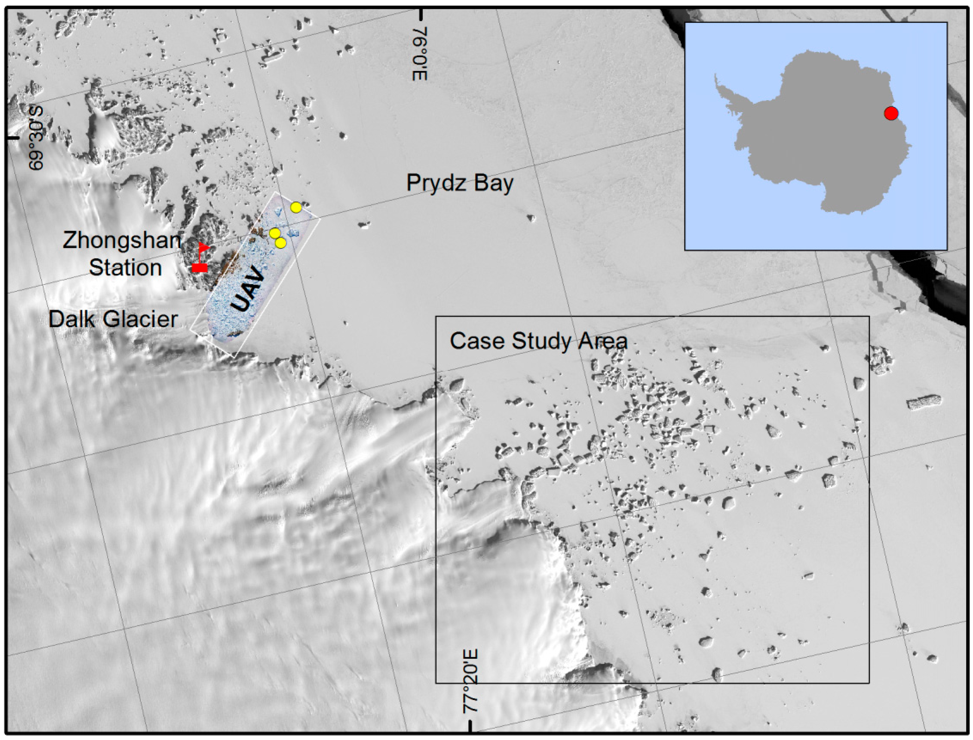
Table 1), for the bi-temporal iceberg freeboard measurements. We applied the bi-temporal shadow freeboard method across an 860-km² iceberg region near the Chinese Zhongshan Station, in Prydz Bay, East Antarctica. We identified more than 400 icebergs with sizes ranging from 0.001 to 0.7 km
2 (
Figure 1).
Three capsized icebergs near the case study area were observed by the Polar Hawk-III unmanned aerial vehicle (UAV) on 13 December 2016, collected in the Prydz Bay near the Chinese Zhongshan Station. The Polar Hawk-III is a fixed-wing UAV with an integrated remote sensing system. We used the freeboards derived from the 0.17-m resolution DSM generated using the UAV data for the method validation. The UAV freeboard was calculated as the elevation difference between the iceberg and its surrounding sea ice. The DSM was generated by gridding the 3D model. The image obtained by the UAV was used to generate a high-quality sparse 3D point cloud after image key-point extraction and an initial alignment, and then, on-board global positioning system (GPS) and inertial measurement unit (IMU) information were employed to geo-reference our data [
27]. The sparse clouds were manually filtered, followed by a densification using a multi-view stereopsis (MVS) algorithm to generate the high-quality dense point cloud. The dense point cloud was used to construct a DSM, from which a digital orthophoto map (DOM) was created with a 0.17-m pixel resolution. The vertical precision of the DSM was about 1 m and the estimated freeboard precision was about 1.4 m. A more in-depth description of the workflow and accuracy of these results can be found in Li et al. [
27].
3. Methods
3.1. Iceberg Freeboard Measured by the Shadow-Height Method
The freeboard of an iceberg surrounded by sea ice can be expressed as follows:
where
Hiceberg and
Hseaice are the freeboards of the iceberg and the sea ice, respectively; and
H is called the shadow freeboard of the iceberg (i.e., the difference between the elevations of the iceberg and the sea ice), which is the height of the iceberg measured using the shadow-height method.
If the shadow length
L of the iceberg on sea ice can be fully measured and the solar elevation angle
θ causing the shadow is known, the shadow freeboard
H can be calculated using simple trigonometry, as follows:
3.2. Shadow Length Determination from Remote Sensing Image
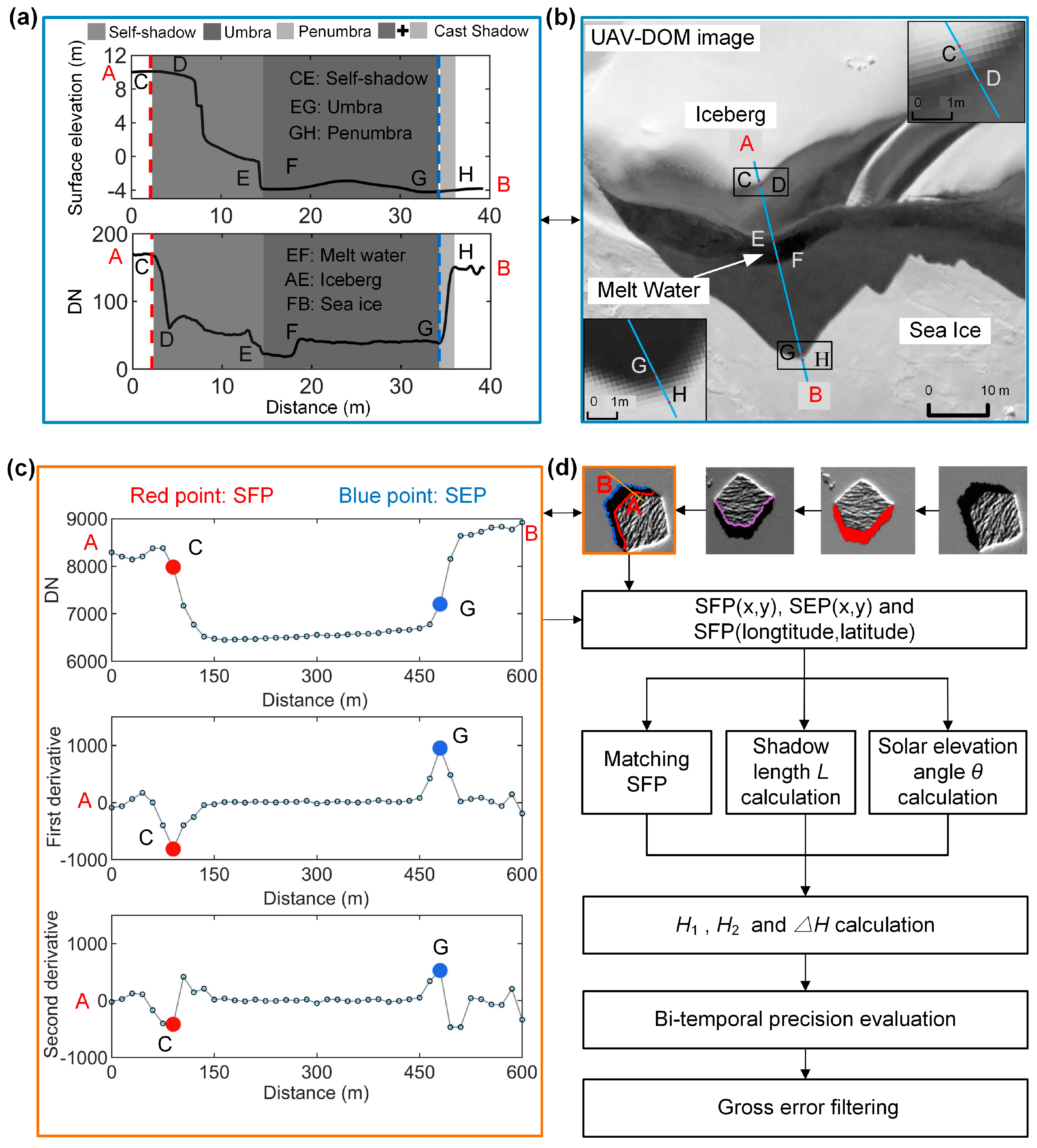
Shadows in remotely sensed imagery occur when objects totally or partially occlude the direct light coming from a source of illumination, which includes cast shadows (shadows cast on the ground, or on other objects, by high-rise objects), and self-shadows (the part of the object that is not illuminated by direction light). A cast shadow consists of two parts: the umbra and the penumbra. The umbra is created when direct light is completely blocked by an object, and the penumbra is created by something partially blocking the direct light [
33,
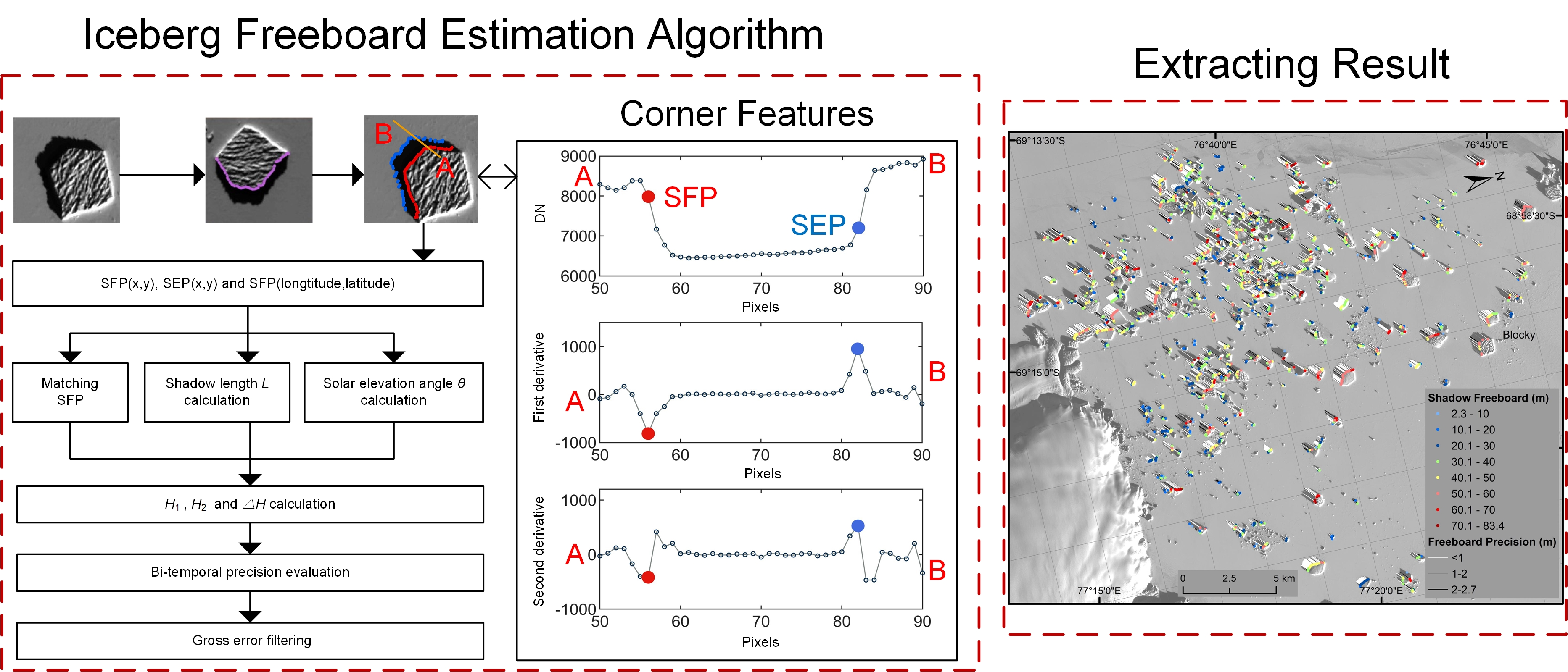
34]. The distance from the iceberg’s peak point (called the shadow formation point, SFP) along the shaded area to the end point (called the shadow edge point, SEP) of the umbra is the extracting length required in the shadow-height method. The elevation and digital number (DN) profile of the iceberg along a beam of direct light is shown in
Figure 2a,b.
The gray DN-profile presents a U-shaped distribution showing that the shaded area is distinctly darker than the non-shaded area (
Figure 2a,c), which is the basis for our shadow detection using the simple histogram thresholding method [
35]. The DN-value sharply decreased after the SFP and the DN-value sharply increased after SEP, usually named as corner features [
36], which provides the basis for precisely identifying the SFPs and the SEPs. Corner features are used to detect points where the curvature and the gradient magnitude are simultaneously high [
37,
38]. In particular, the curvature of the discrete point is approximately equal to its second-order derivative (as shown in
Figure 2c). Thus, we combined the simple histogram threshing method and the corner features to accurately determine the iceberg shadow length.
3.3. Solar Elevation Angle Calculation
The Landsat-8 metadata only provides the solar elevation and azimuth angles of the scene center point. The solar elevation and azimuth angle differences between the scene upper left corner and the scene lower right corner are up to 3 and 7 degrees, respectively. The freeboard measurement error caused by this would be more than several meters. Therefore, the solar elevation angle is calculated in each SFP to account for the differences in the accurate geographical coordinates of the SFPs, the date, and the time of the image acquisition. We used the Solar Position Algorithm (SPA) distributed by the National Renewable Energy Laboratory (NREL) Solar Radiation Research Laboratory [
39,
40] to calculate the solar elevation and azimuth angles of the SFPs. We derived the solar elevation angle and the solar azimuth angle from the accurate geographical coordinates of the SFPs, the date, and the time of image acquisition. The SPA algorithm was used to calculate the solar elevation and azimuth angles in the period from the year −2000 to 6000, with uncertainties of ±0.0003 degrees based on the date, time, and location [
41], which contributes a freeboard measurement error of less than 0.001 m. Thus, we could ignore the error in the measured height resulting from the solar elevation angle.
3.4. Data Filtering by Bi-Temporal Evaluating Method
The bi-temporal shadow freeboard measurement aims to evaluate the precision and to automatically filter out the gross error. With negligible iceberg movement in the two continuous phase images, we measured shadow freeboard
H of the matching SFP two times at different solar elevation angles. The difference between the two freeboard measurements,
, is calculated as follows:
The combined standard uncertainty with correlated input quantities,
, is determined by the combined standard uncertainty of
H1 and
H2,
and
, and the correlation coefficient between
and
,
.
Since we ignored the solar elevation angle error,
and
are determined by the shadow length uncertainty (i.e., shadow length precision) and by the solar elevation angle, as follows:
When the solar azimuth angles are equal or very close to each other, it can be assumed that
. Then,
For any given , can be obtained by iterations under the assumption of initial and . Then, we calculated the correlation between the probability distribution of the observed at the given interval and the modeled following a random normal distribution with a mean of and a standard deviation (σ) of the at a given interval in the interval of (hereinafter referred to as the P-correlation). The fixed and for subsequent precision evaluation were the iterative calculation results of and at the , where the P-correlation coefficient reached the maximum.
Then, the measurement uncertainty of shadow length,
, in the interval of
, is calculated as follows:
where
is the σ of the
. The expected uncertainty of shadow length,
, is
, which is the σ of the modeled normally distributed shadow length error in the interval of
. The relative difference between the
and
is as follows:
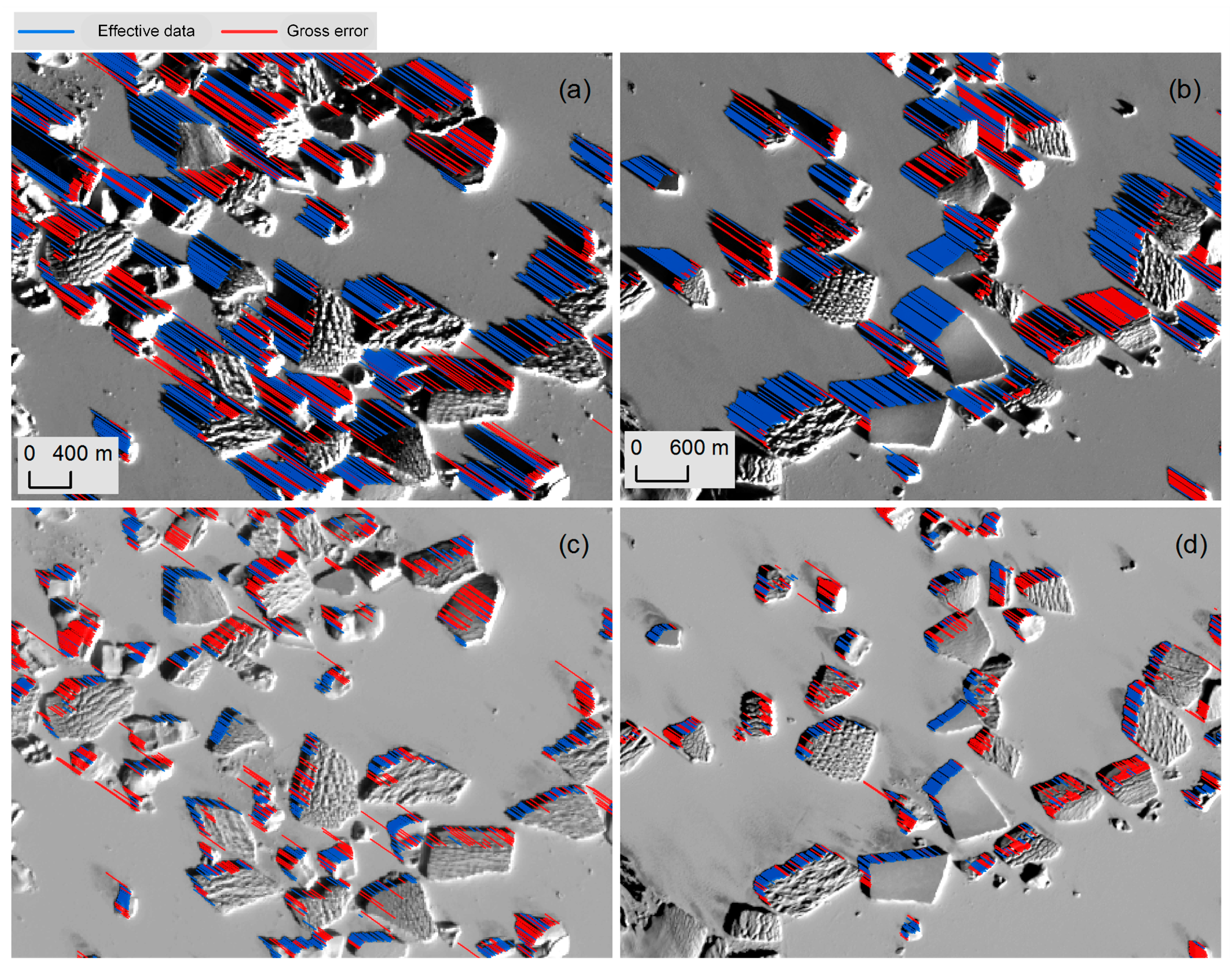
was considered to be acceptable when was less than 0.1 and the P-correlation coefficient was greater than 0.8. Then, we selected the freeboard data with the expected available freeboard precision of . The effective data had a shadow length precision of better than 2 pixels (30 m), and the gross error without the effective interval was filtered out.
3.5. The Process of Automatic Bi-Temporal Shadow Freeboard Measurement
We developed an automatic process to measure the shadow freeboard
H. The proposed process has six steps: (1) automatic extraction of the iceberg’s shadow regions, filtering the shadows fully on icebergs and locating initial SFPs (SFP0s); (2) accurate determination of the locations of SFPs and SEPs using the corner features of interpolated DN-profile along the exact shadow direction of SFP0s (
Figure 2c); (3) bi-temporal SFPs matching; (4)
H1,
H2, and
calculation; (5) bi-temporal precision evaluation; and (6) gross error filtering. The general framework of the proposed method is shown in
Figure 2d.
Shadow region detection, shadow filtering, and SFP0s acquisition. We automatically extracted the shadow regions from the Landsat-8 panchromatic images using a histogram thresholding method. This method is based on the fact that the shaded areas are distinctly darker than the nonshaded areas. The shadow threshold is simply visually interpreted using the three-dimensional (3D) analyst tool. The full shadows on the icebergs were not our aim for iceberg freeboard measurement. These shadows could be filtered easily by the thresholds of the area and perimeter area ratio of the shaded areas. In this process, we also filtered out some of the shadows that were fully on the sea ice of the small icebergs with size less than 0.002 km
2. Then, along the direction of the light, the first pixel of the shadow we obtained was the initial SFP (SFP0). The initial direction of the light is calculated based on the solar elevation and azimuth angles of the center point of the iceberg area. However, automating this process is complicated. If we redirect the shadow to the south of the image (e.g., parallel to the y-axis in the image coordinate system, as shown in
Figure 2d) through rotation, automatically obtaining the SFP0 becomes easy. Thus, first we rotated the original image to redirect the shadow to the south of the image. To avoid losing the coordinate information, we rotated the original x, y coordinate images. The Landsat-8 Level 1T image products for Antarctica are defined in the Polar Stereographic Projection with −71°S standard latitude to reduce the area distortion in the polar regions [
42]. The image rotation angle is
, where
α is the solar azimuth angle and
β is the longitude at the center of the iceberg region. Then, we automatically determined the initial SFP0s and SEP0s for the shadow length calculation as the first and end pixels of the shadow regions from the north to south of the rotated binary shadow image and obtained their x, y coordinates from the rotated x, y coordinate images.
Accurate determination of the SFPs and SEPs. To further accurately determine the SFPs and SEPs, we interpolated the DN-profile of the shaded area with a step length of 10-m and their neighboring nonshaded areas crossing every SFP0 along the shadow orientation. We accurately determined the shadow orientation using the SFP0’s longitude and the solar azimuth angle that we derived from the extracted geographical coordinates of the SFP0s using the NREL’s SPA. The angle between the direction of the shadow’s orientation and the y-axis direction used to obtain the SFP0’s DN-profile was calculated as follows:
where
αi is the solar azimuth angle of the SFP0s, and
βi is the longitude of the SFP0s. Thus, the purpose of the image rotation was to obtain the initial SFP0 and its corresponding shadow direction. Then, the accurate SFPs and SEPs were extracted using the corner features (
Figure 2c).
Bi-temporal SFPs matching. We determined the two bi-temporal SFPs as the bi-temporal matching SFPs when the distance between them was less than the threshold of 15-m.
H1, H2, and calculation. According to the accurate location of the matching SFPs and their related SEPs, we calculated their shadow lengths, the solar elevation angles of the SFPs, and the single-shadow heights of H1 and H2. is the difference between H1 and H2.
Bi-temporal precision evaluation. We estimated the shadow length precision and calculated the freeboard precision according to the method described in
Section 3.4.
Gross error filtering. We filtered out the gross error using the expected shadow length precision.
5. Validation
In the study area, we obtained 9294 pairs of H9/16–H8/29, 8670 pairs of H9/30–H8/29, and 9218 pairs of H9/30–H9/16 bi-temporal matching SFPs, and 6313 tri-temporal matching SFPs from the single shadow freeboard measurements of H8/29, H9/16, and H9/30, respectively. The solar elevation angles of the H8/29, H9/16, and H9/30 were 5.17 ± 0.05°, 11.16 ± 0.05°, and 17.50 ± 0.05°, respectively. Their solar azimuth angles were 47.6 ± 0.05°, 49.24 ± 0.05°, and 48.36 ± 0.05°, respectively, which were so similar that we could ignore the shadow length precision differences among H8/29, H9/16, and H9/30.
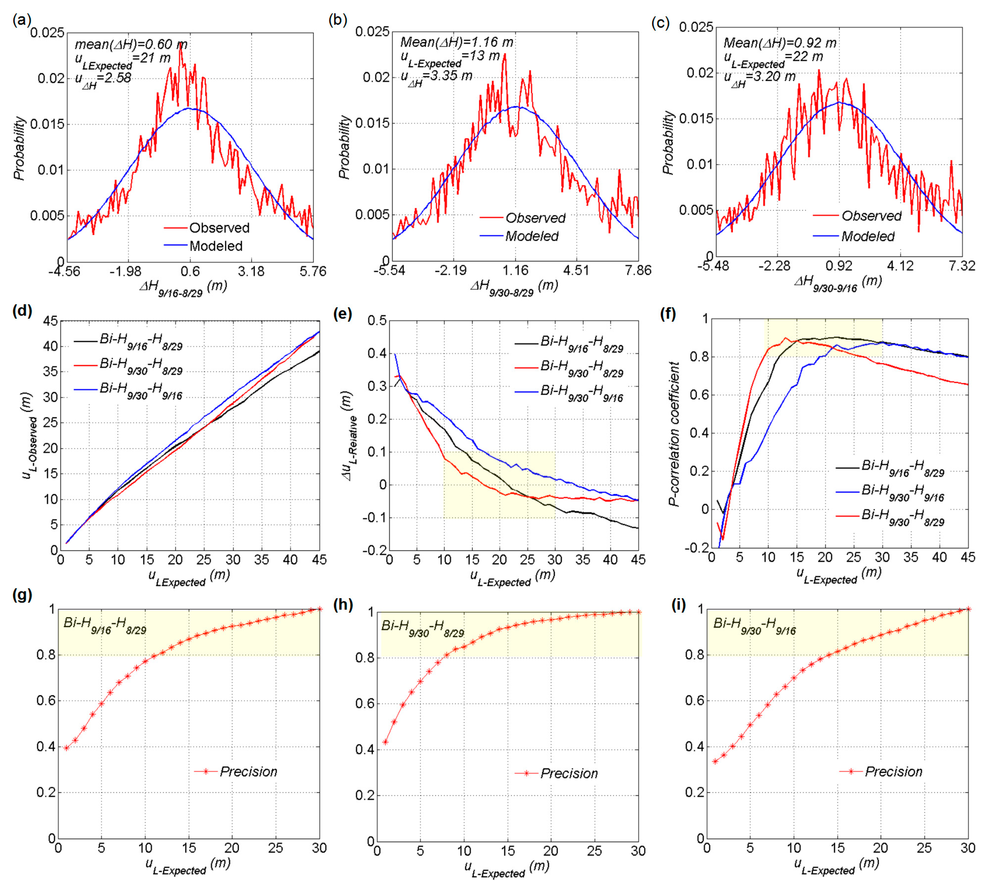
Our test showed that the best fits of the P-correlations between the observed
,
, and
and a modeled normally distributed
(
Figure 5a–c) appeared at the
of 21 m, 13 m, and 22 m, respectively. Their correspondence
r(
H1,
H2) values were 0.986, 0.968, and 0.976, respectively. The bi-temporal measurements of the
H9/16–
H8/29 and
H9/30–
H9/16 had similar time intervals and their bi-temporal evaluations had more identical and consistent results. The
,
, and
are 0.60 m, 1.16 m, and 0.92 m, respectively, which indicated the system errors of the shadow length are 5.5 m, 5.0 m, and 7.1 m (all less than half a pixel) rather than the freeboard change due to snowfall, the basal freezing of iceberg or the basal melting of the sea ice. This is because snowfall both increases the iceberg and sea ice elevation, which contribute little shadow to the freeboard of the iceberg. Such shadow freeboard changes due to basal freezing of the iceberg would cause sea ice breakage that we did not observe. The possible changes in the sea ice freeboard in 32 days is on the order of less than 0.1 m. With known
and
r(
H1,
H2), we calculated the variations of the
,
and P-correlation coefficient with the
(
Figure 5d–f). The analysis of variance (ANOVA) test results were consistent with the expectation that there were no significant differences (
p > 0.05) among the three bi-temporal
or between any two when
ranged from 0 m to 45 m at 1-m intervals. These results demonstrated the effectiveness of the bi-temporal method for shadow length precision evaluation.
Our required
range should be less than 30 m (2 pixels), and the effective shadow precision range judged by the
less than 0.1 was consistent with those judged by the P-correlation coefficient greater than 0.8 (
Figure 5e,f). The effective
ranges of the bi-
H9/16–
H8/29, bi-
H9/30–
H8/29, and bi-
H9/30–
H9/16 were 14–30 m, 10–26 m, and 19–30 m, which indicated that we could select available freeboard data with expected precision within these ranges. Furthermore, we tested the precision of our proposed evaluation method by cross-validation of the three bi-evaluations. The precision of one bi-evaluated set was calculated as
P =
NuL/
UNuL, where the
NuL was the number of one bi-evaluated set and
UNuL was the number the union of the three bi-shadow evaluated sets. Excluding the gross error, there were 2728 of tri-temporal matching SFPs with
better than 30 m. As expected, these results showed that high-precision appeared in the effective ranges of shadow length precision (
Figure 5g–i).
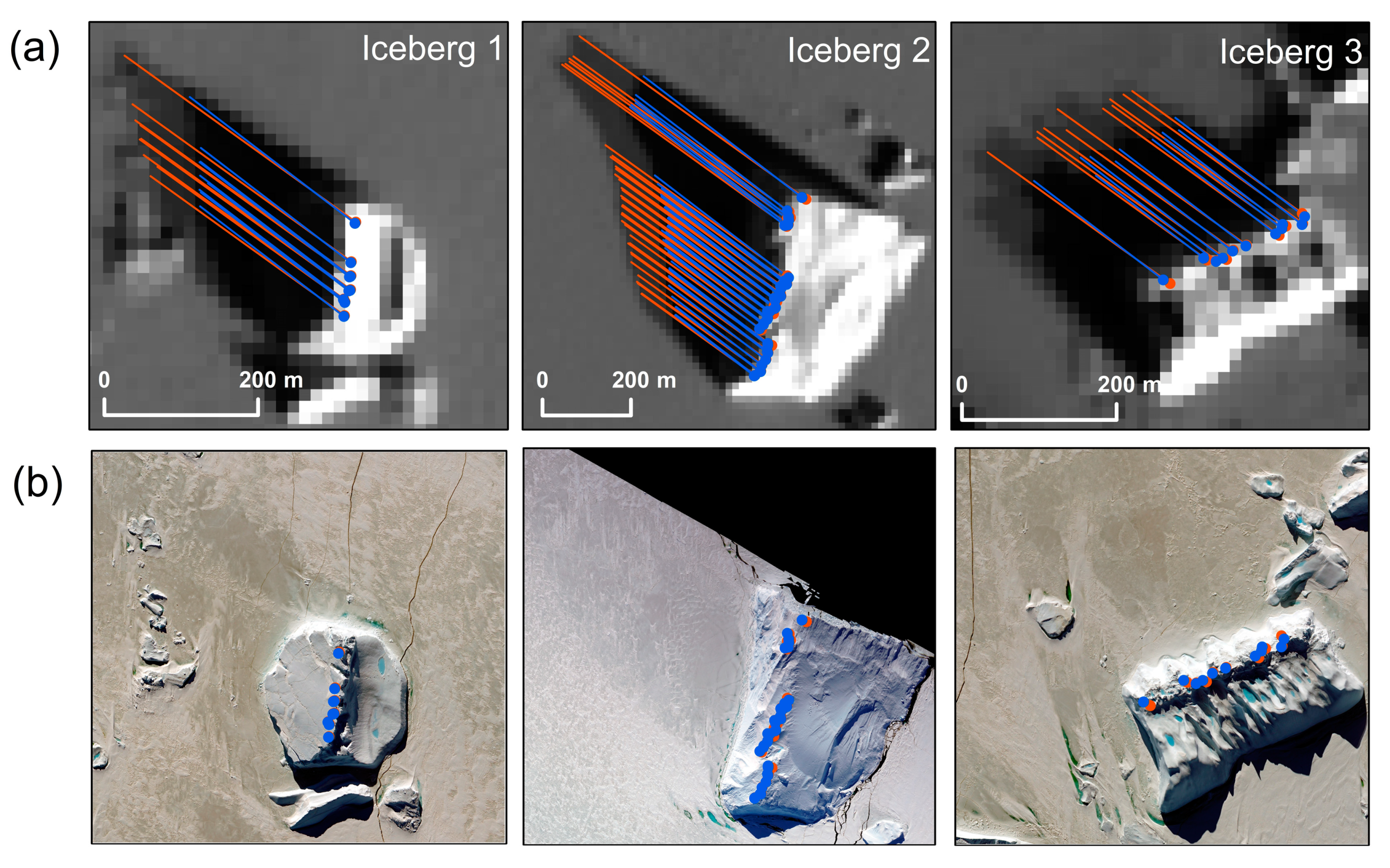
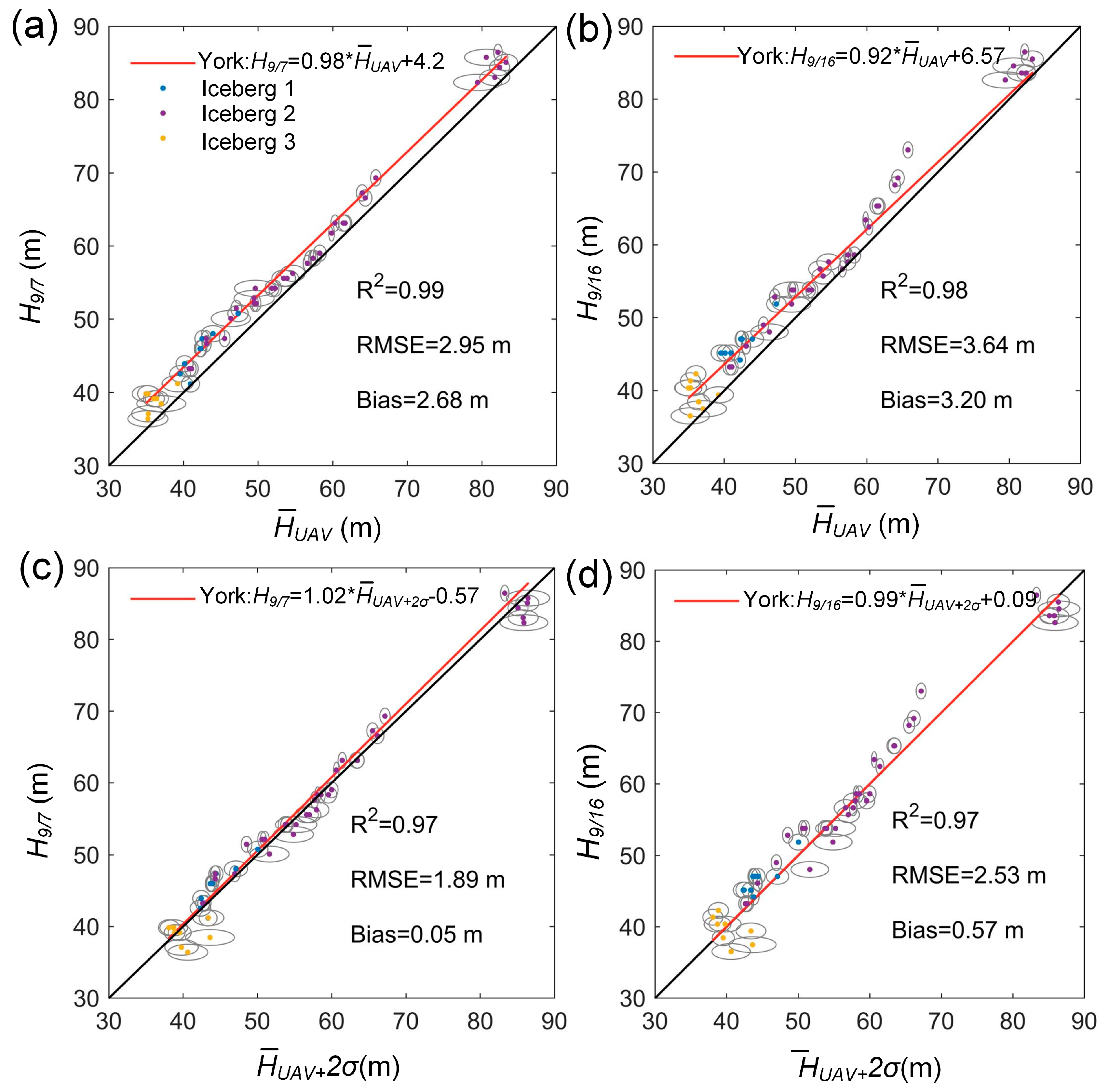
To further validate freeboard precision, we compared the effective shadow freeboard
H9/7 and
H9/16 with the UAV freeboard of
HUAV12/13. The former Landsat-8 freeboards had the expected precision of 2.1 m and 3.0 m, whereas the latter had an estimated precision of 1.4 m. We used the 51 effective matchings SFP pairs of H
9/7 and H
9/16 on the three UAV-investigated icebergs for validation (
Figure 6a,b). The locations of the SFPs agreed well with the iceberg peaks along with the light directions. The spatial resolution of the UAV image of 0.17-m was about 100 times higher than the 15-m Landsat-8 panchromatic image. The average standard deviation of the
HUAV12/13 measurements within an SFP grid was up to 1.32 m (
n = 51). The shadow freeboards
H9/7 and
H9/16 were highly correlated with the
and the
(r > 0.99) (
Figure 7). The shadow freeboards
H9/7 and
H9/16 had better York’s linear fits with errors [
43] and a smaller basis with the
(
Figure 7c,d). These results indicated that the shadow freeboard better represented the peak profile within the area of the SFP grid. Thus, the precision of the shadow freeboards of
H9/7 and
H9/16 validated by UAV freeboards were 1.89 m and 2.53 m, which were within the expected precision by the bi-temporal measurement.
6. Discussion and Conclusions
Our proposed method provided a general methodological framework for various iceberg freeboard extraction using freely available Landsat-8 OLI, 15-m bi-temporal panchromatic image shadows. This method has the advantage that it is simple to model, required less manual intervention, and has a considerably high precision.
The combination of the histogram thresholding method and the corner features of the shadow’s DN-profile was able to break through the difficulties caused by the complex interactions of geometry, albedo, and illumination and accurately determined the iceberg shadow length. The automatic shadow length acquisition was easily achieved by redirecting the shadow to the south. We precisely estimated the shadow freeboard based on the previously noted precise shadow length extraction and the SPA’s accurate solar elevation angle calculation.
For many reasons, the full length of the iceberg shadow cannot always be obtained completely, for example, shadows can be obscured by the other icebergs, which leads to ineffective shadow freeboard measurement. Manually filtering the gross error can be time-consuming and laborious, especially for a large number of measurements. Our proposed bi-temporal evaluation method successfully evaluated the measurement precision and filtered out the gross error. Its effectiveness was tested and validated by generating the freeboard data of the icebergs in an area in Prydz Bay, East Antarctic, using the four Landsat-8 panchromatic images and the UAV freeboard data. The bi-evaluation method enabled us to obtain the system error of the shadow length measurement of this method, which is less than half a pixel. Furthermore, it enabled us to select available data with expected precision within the effective precision range. The effective precision range was dependent on the minimum solar elevation angle of the bi-temporal freeboard measurements and the time interval between the two measurements. We expect to select out higher precision data from the bi-temporal measurements with lower minimum solar elevation angle and longer time interval. The bi-temporal evaluation has a harmless disadvantage. According to Equation (6), the precision of the single shadow freeboard was more likely to be underestimated when there was little systematic error. This indicated that some effective data were filtered out as gross errors. Tri-temporal evaluation using three shadow freeboard measurements may be effective in avoiding this problem to some extent, but it faces the difficulty of data acquisition.
The freeboard changes of iceberg and sea ice had a rather small impact on the bi-temporal shadow freeboard estimation and validation when the iceberg was trapped in sea ice from August to December. Tournadre et al. [
19] ignored the iceberg freeboard change when the iceberg was trapped in sea ice and regarded the change of freeboard as a function of accumulated days of positive sea surface temperature. Most of the observed freeboard change of iceberg was due to melting [
19]. Neither the cross validation using the bi-temporal Landsat-8 freeboards nor the comparison between and the UAV freeboard and the Landsat-8 shadow freeboard showed a decrease in the freeboard over time, which indicates that the impact of iceberg melting can be ignored. The long-term sea ice thickness (including ridges) in the Southern Ocean has been reported to be 0.87 ± 0.91 m [
44]. Assuming that the ratio of the thickness of the ice below sea level to the freeboard of the sea ice (i.e., the thickness of ice plus snow above sea level) is 7 based on the mean ratio of those of the snow-free ice and the ridged ice are 9 and 5.1, respectively [
44], the mean freeboard of the sea ice is 0.11 ± 0.12 m, which is relatively small compared to the freeboard of the iceberg and its measurement error obtained from the shadow height. Therefore, the impact of the freeboard change on the bi-temporal elevation and precision validation can be ignored. Notably, the shadow freeboard is not the full freeboard of iceberg and the freeboard of the sea ice is relatively small but cannot be ignored in the estimation of the freeboard of iceberg.
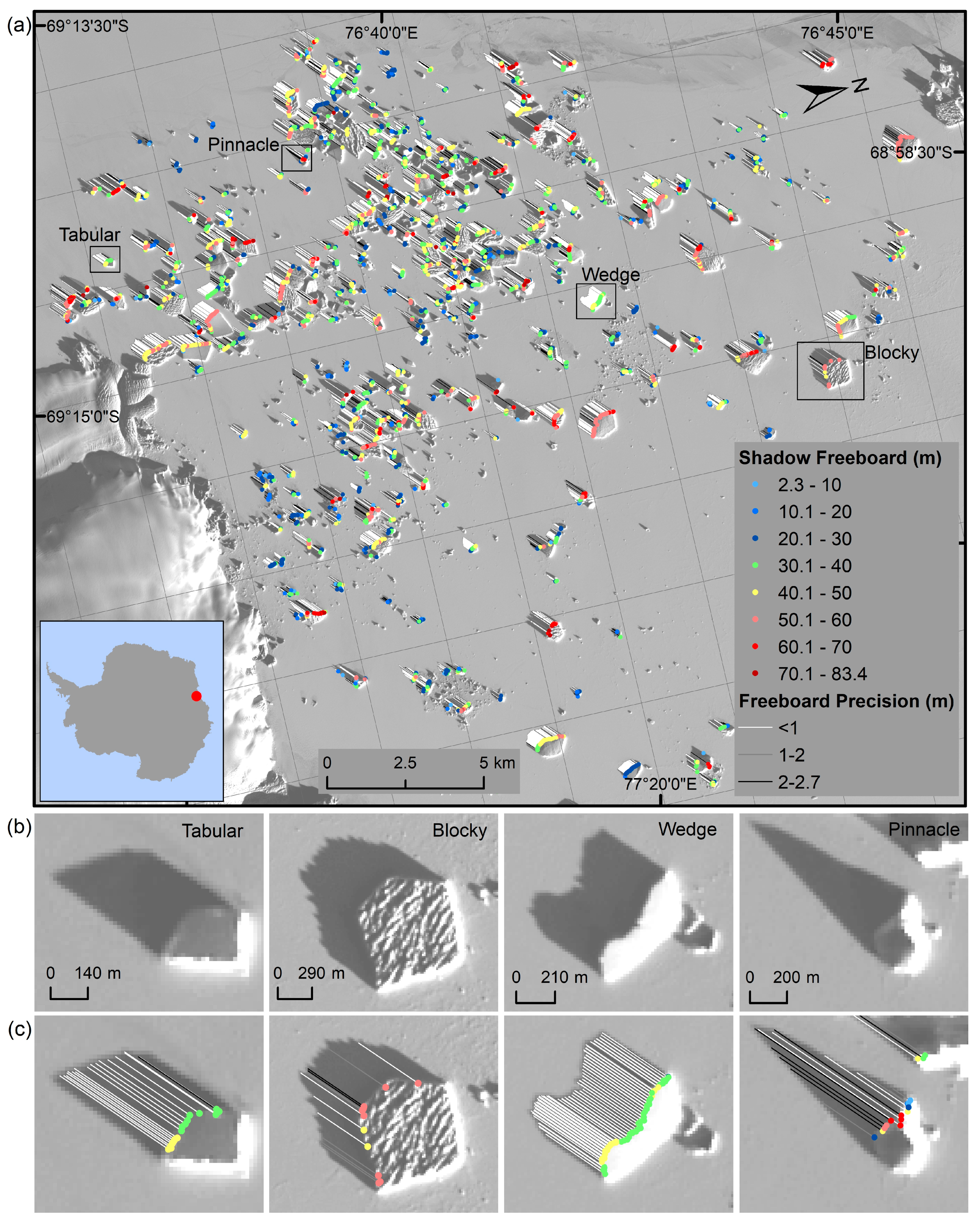
The DSM generated from high resolution optical images can be used to measure the full freeboard of the entire iceberg just as the UAV freeboard used in our validation. However, this method has significant limitations in terms of data acquisition at a continental scale. Like the constraint of the altimeter method, the shadow height method only measures a certain profile of the iceberg. Unlike the altimeter, which measures a profile of iceberg along the ground track, this method measures the highest profile along the direction of the sun’s rays. For the average freeboard estimation of a tabular or block iceberg (
Figure 3b), the errors could be offset by multiple measurements around the half-edge of the iceberg. For the average freeboard estimation of an iceberg with distinct elevation differences, such as a pinnacle or capsized iceberg, it was likely to be overestimated. Fortunately, the tabular or block icebergs accounted for the majority of the total Antarctic iceberg area. The disadvantage became an advantage in the iceberg freeboard change investigation. The high points of the iceberg were likely to be observed repeatedly by the shadow-height method even if the iceberg drifted or rotated, whereas the track profile rarely could be observed repeatedly by the altimeter [
21]. This indicates that the shadow height method can be used to detect the freeboard change of an iceberg, and then its basal melting.
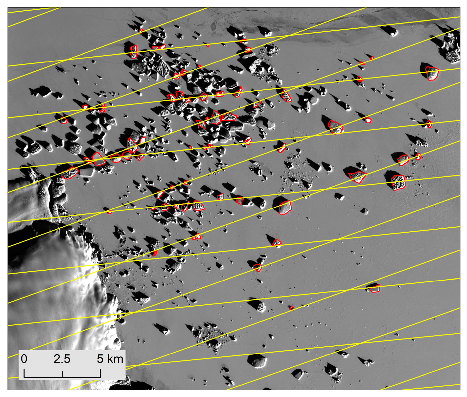
Further, unlike the altimeter, which only measures the icebergs covered by the orbit tracks, the optical image can measure nearly all of the icebergs with full shadow using the shadow height method. For example, the orbit spacing of the ICESat-2 satellite is about 6.6 km at 70° S/N. Only 76 icebergs could be tracked by all of the ICESat-2’s repeated orbits in our case study area, while 376 icebergs could be effectively measured using the Landsat-8 images (
Figure 8). Furthermore, the other optical satellite images with higher resolution (such as the Sentinel-2 10-m visible images, and the WorldView-2 0.5-m images) could also be used to measure the freeboard of the icebergs using the shadow height method. Therefore, it can fill the significant gaps resulting from the insufficient altimeter coverage of the icebergs in the Southern Ocean. However, the shadow freeboard method depended on sea ice coverage and its precision depended on the solar elevation angle, which restricted its applicability. The optical remotely sensed data could be used in the shadow freeboard method, which was also affected by cloud cover. Thus, this method could not replace the altimeter method but provided a good supplementary means.
The method presented in this study is a part of ongoing work to generate a high-quality freeboard dataset of the various Antarctic icebergs. In the future, we plan to estimate basal melting of the icebergs using repeated shadow freeboard measurements.


 ,
, 


