STAIR 2.0: A Generic and Automatic Algorithm to Fuse Modis, Landsat, and Sentinel-2 to Generate 10 m, Daily, and Cloud-/Gap-Free Surface Reflectance Product

Abstract

Remote sensing datasets with both high spatial and high temporal resolution are critical for monitoring and modeling the dynamics of land surfaces. However, no current satellite sensor could simultaneously achieve both high spatial resolution and high revisiting frequency. Therefore, the integration of different sources of satellite data to produce a fusion product has become a popular solution to address this challenge. Many methods have been proposed to generate synthetic images with rich spatial details and high temporal frequency by combining two types of satellite datasets—usually frequent coarse-resolution images (e.g., MODIS) and sparse fine-resolution images (e.g., Landsat). In this paper, we introduce STAIR 2.0, a new fusion method that extends the previous STAIR fusion framework, to fuse three types of satellite datasets, including MODIS, Landsat, and Sentinel-2. In STAIR 2.0, input images are first processed to impute missing-value pixels that are due to clouds or sensor mechanical issues using a gap-filling algorithm. The multiple refined time series are then integrated stepwisely, from coarse- to fine- and high-resolution, ultimately providing a synthetic daily, high-resolution surface reflectance observations. We applied STAIR 2.0 to generate a 10-m, daily, cloud-/gap-free time series that covers the 2017 growing season of Saunders County, Nebraska. Moreover, the framework is generic and can be extended to integrate more types of satellite data sources, further improving the quality of the fusion product.

1. Introduction

High spatiotemporal-resolution time series of optical satellite data are critical for the effective modeling and precise monitoring of land surface features and processes. Rich spatial information and temporal dynamics of surface reflectance can improve the output accuracy of several applications, including land cover mapping [1,2], evapotranspiration estimates and crop monitoring [3], crop yields estimates [4,5,6,7,8], and urban applications [9,10].

The currently available satellite missions, however, cannot simultaneously achieve both high spatial resolution and high revisiting frequency due to the tradeoff between scanning swath and pixel size [11]. For example, MODIS, AVHRR, and SeaWiFS provide daily images but their spatial resolutions ranges from 250 m to 1 km. On the other hand, Landsat and Sentinel-2 deliver a finer spatial granularity (e.g., 10–30 m), but in a lower sampling frequency (from days to weeks). The revisiting frequency can extend longer due to clouds, cloud shadow, atmospheric conditions, and satellite sensor damages (e.g., the failure of the scan-line corrector (SLC) of Landsat 7) [12]. Therefore, lack of dense time series with high spatial resolution becomes the one major obstacle, particularly considering the need for precision agriculture and capturing in field variabilities [13,14].

Data fusion algorithms have been developed for integrating multiple optical satellite sources and generating high spatiotemporal data from simple [7,15] to more complex approaches [3,16]. Notable examples, among others, include the STARFM algorithm [17] and its successor Enhanced STARFM (ESTARFM) [18] that blend Landsat and MODIS datasets. These methods generally follow similar principles: (i) using matching pairs of coarse- and fine-resolution images from the same date; (ii) considering a coarse-resolution image of the target date; and (iii) generating a fine-resolution image for the target date using a weighted neighborhood voting process. Several attempts have been proposed to improve STARFM and ESTARFM, and the details of these algorithms can be found in [19]. The major limitation of methods sharing the same spirit as STARFM is the need for the manual selection of matching pairs of cloud-free images acquired on the same date, which significantly hinders their applicability in generating dense high-quality time series of surface reflectance data. To address these challenges, we previously developed STAIR, a generic and fully-automated method for fusing multiple sources of satellite data and generating a cloud-/gap-free data with both high frequency and high resolution [20]. STAIR benefits from a filling algorithm that can effectively impute the missing pixels (due to cloud or sensor damage) as well as an automatic fusion framework that does not require the manual selection of matching pairs of cloud-free images as input. The advanced performances of the algorithm for fusing Landsat and MODIS data and generating 30-m daily surface reflectance data has been validated over a large agricultural landscape [20]. The availability of Sentinel-2 data has created new opportunities to enhance the spatial resolution of the Landsat-based fused products. In particular, the recent Harmonized Landsat and Sentinel-2 (HLS) project combines surface observations from Landsat 8 and Sentinel-2, with necessary radiometric and geometric corrections, to provide a near-daily surface reflectance dataset at 30-meter resolution [21].

While the fusion of two satellite sources has been extensively studied, the increasing number of satellite missions and their complementary characteristics open new avenues of the fusion of more than two satellite datasets. For example, CESTEM (a CubeSat enabled spatiotemporal enhancement method) was proposed to integrate three satellite sources, including MODIS, Landsat 8, and PlanetScope [22]. However, the main purpose of CESTEM is to use Landsat and MODIS data to correct for radiometric inconsistencies between CubeSat acquisitions of PlanetScope images. Additionally, CESTEM is not able to remove and impute cloud pixels in the input images, and thus still requires manual selection of near-coincident, cloud-free input images. To the best of our knowledge, to date, the fusion of a more rigorously calibrated satellite data (e.g., Sentinel-2) with MODIS and Landsat has not been explored in existing works.

In this work, we introduce STAIR 2.0, an extension of STAIR which provides a framework to fuse three satellite data sources (namely, Landsat, MODIS, and Sentinel-2), to generate 10-m and daily surface reflectance data (Figure 1). We quantitatively evaluate the quality of the fusion results and show the advantages of using three satellite data sources as compared only using two types of satellite data.

2. Materials and Methods

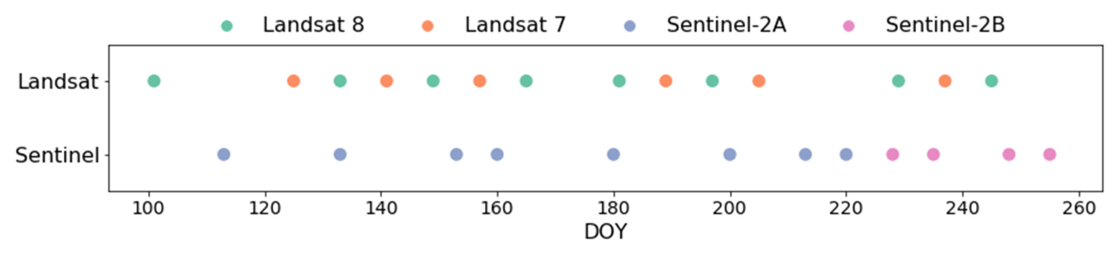
2.1. Dataset

We aimed to build fusion data using MODIS, Landsat, and Sentinel-2 images of Saunders, NE, in 2017 to evaluate the performance of STAIR 2.0. We selected MODIS, Landsat, and Sentinel-2 surface reflectance data that cover various dates in the growing seasons from 1 April to 1 October across six spectral bands (red, green, blue, NIR, SWIR1, and SWIR2). More specifically, we collected MODIS MCD43A4 products [23,24], Landsat data (Landsat 5, 7, and 8) [25,26], and Sentinel-2A and -2B Level 1C products for the year 2017 that cover Saunders, NE. The MODIS product has a frequent (daily) revisit cycle, but a coarse spatial resolution (500 m). While the Landsat product has a higher spatial resolution (30 m), its temporal resolution is relatively lower (16-day revisit cycle), and the images in Landsat are often cloud-contaminated. The Sentinel product has a 20-day revisiting frequency, and the spatial resolution is 10 m for the RGB and NIR bands and 20 m for SWIR1 and SWIR2 bands. We further used the Sen2Cor processor [27] to perform the atmospheric, terrain, and cirrus correction of Sentinel-2 Level 1C products, which also resampled the SWIR1 and SWIR2 bands to 10-m resolution. Radiance calibration and atmospheric corrections were applied to both Landsat and MODIS surface reflectance data, and only clear-day pixels are retained for fusion. For Landsat data, we filtered out cloudy pixels using the cloud mask band in the surface reflectance product, while for MODIS data only pixels flagged as “good quality” were used for fusion. We excluded scenes with the fraction of cloud pixels greater than 75%, as the non-cloud pixels in those images are often low-quality and inaccurate. SWIR1 and SWIR2 bands in sentinel-2 were resampled to 10-m resolution before the fusion.

2.2. Data Preprocessing

2.2.1. Spatial Co-Registration

To correct the spatial shifts existing in MODIS, Landsat, and Sentinel-2 images, we used Landsat images as the reference and performed spatial co-registration to correct the pixel coordinates of MODIS and Sentinel-2 images. Due to the difference in spatial resolutions, we used different registration approaches for MODIS–Landsat and for Sentinel–Landsat.

We first co-registered each Landsat–MODIS pair acquired on the same day by enumerating all the possible shifts of the Landsat image in each of the four cardinals and four ordinal directions. In each direction, we shifted the image by at most 20 pixels. This choice was made based on the fact that one MODIS pixel approximately corresponds to one block of 17 × 17 pixels in the Landsat image. The optimal shifting that maximized the correlation between the shifted Landsat and the MODIS images was then applied to co-register the Landsat–MODIS pair.

We used an algorithm based on tie point detection to perform co-registration between Landsat and Sentinel 2 images. We first used the Scale-Invariant Feature Transform (SIFT) [28] to find image key points in Landsat and Sentinel 2 images. For each key point on the Landsat image, we then searched for potential matching key points in the Sentinel 2 image. The matching criteria for the key points included: (1) close pixel distance; and (2) similar corner orientation. The matchings were used to fit a transformation of geolocation. In this step, we provided the flexibility of three methods to perform the co-registration to better accommodate different use cases: (1) assume a constant offset vector across the image and derive it by averaging over the shift vector of all matching key point pairs; (2) smooth the spatial variance of shift vectors of the matching key points and perform a 2D interpolation of the shift vector to generate an offset map; and (3) assume affine transformation and fit the following transform using all matching key point pairs

$$d\left(\widehat{p}\right)=w\widehat{p}+\widehat{r}$$

(1)

where $\widehat{p}$ is the position on the image; $d\left(\widehat{p}\right)$ is the offset vector at $\widehat{p}$; $w$ is a 2 by 2 weight matrix; and $\widehat{r}$ is an offset vector. $w$ and $\widehat{r}$ are the fitted values. Finally, the offset map generated by either one of the three methods was applied to the Sentinel 2 image, completing Landsat–Sentinel geometric calibration.

2.2.2. Spectral Adjustment

It is necessary to perform the spectral adjustment of surface reflectance values before the fusion step. There are small differences of wavelengths existing between equivalent spectral bands of Landsat and Sentinel-2 satellite sensors (

Table 1. Band wavelengths (nm) of MODIS, Landsat 5/7/8, and Sentinel-2 satellite sensors.

Band	MODIS	Landsat 5/7	Landsat 8	Sentinel-2
Blue	459–479	441–514	452–512	458–523
Green	545–565	519–601	533–590	543–578
Red	620–670	631–692	636–673	650–680
NIR	841–876	772–898	851–879	785–900
SWIR1	1628–1652	1547–1749	1566–1651	1565–1655
SWIR2	2105–2155	2064–2345	2107–2294	2100–2280

). For example, the central wavelengths of the blue band in MODIS, Landsat 5/7, Landsat 8, and Sentinel-2 are 469, 477, 482, and 490 nm, respectively. Here, we used Landsat images as the reference and adjust the MODIS and Sentinel-2 spectral bands to it. We first used the regression model derived in previous work [29] to transform the surface reflectance values of Landsat 5/7 to the comparable bands of Landsat 8. We then adopted the approach used in previous work [21], which systematically collected Landsat and Sentinel scenes worldwide and built a linear regression model to adjust Sentinel-2 spectral bands to Landsat bands. We applied the same technique to adjust the equivalent spectral bands of Landsat and MODIS datasets.

2.3. Imputation of Missing Pixels

For MODIS, Landsat, and Sentinel-2 images of frequently cloudy regions, there is often a large portion of missing-value pixels being masked out by the cloud mask due to cloud contamination, leaving only a small fraction of pixels unmasked. In addition, Landsat 7 SLC-off data’s utility was greatly limited by the spatial discontinuity (strips) caused by sensor damage. The imputation of missing-value pixels, including cloudy and/or un-scanned pixels, not only helps reconstruct the full view of the region but also facilitates analyses and applications such as the data fusion of multiple satellite images.

Here, we describe our effective algorithm for imputing the missing-value pixels in MODIS/Landsat/Sentinel-2 images caused by clouds or sensor damage. As an overview, the gap-filling algorithm takes as input time-series images of one type of satellite data (MODIS, Landsat, or Sentinel-2), and iteratively fills images in the time series that have missing pixels. At each iteration, two images are processed: an image with missing pixels (hereinafter, target image) and the temporally closest image that has valid non-missing pixel values (hereinafter, reference image) at the missing regions in the target image. Missing pixels in the target image are first filled by the alternative pixels from the same land cover region in the reference image, and then adjusted by a pixel-wise correction step, which improves the filling quality. The imputation approach of STAIR 2.0 has improvements in both efficacy and efficiency as compared to that of STAIR. First, STAIR 2.0 additionally uses the similarity between time series of pixels to identify similar neighborhood pixels to correct filled values, which makes the gap-filling more robust and accurate. Second, the gap-filling process is parallelized on multiple CPU cores, speeding up the process by up to 20 times.

2.3.1. Step 1: Segmentation of Land Covers

A single satellite image often contains heterogeneous land cover types, and each type may exhibit a unique temporal changing trend in the time series. Considering these differences in changing patterns of heterogeneous pixels, we thus filled the missing pixels of each group of homogeneous pixels separately in the target image. For this purpose, we first applied a clustering algorithm to partition an image into multiple segments, with each segment containing a set of homogeneous pixels corresponding to a specific type of land cover. In contrast to classical clustering workflows where the number of segments ($N_s$) needs to be pre-specified, here we also automatized the algorithm in a way such that it can adaptively choose a proper value of $N_s$ to segment the image. In this work, the k-means clustering algorithm [30] was applied to partition the image into multiple segments of homogeneous pixels, with each segment corresponding to a certain land cover. To automatize the selection of the number of segments ($N_s$) that optimally explains the heterogeneity of land covers in an image, we used gap statistic, an index derived in [31], to quantify the dispersion of the image segmentation results with their expected values under a null reference distribution of the data (a random image with no obvious clustering). Generally, a higher gap statistic indicates the segmentation that better captures the grouping patterns in the image. In this work, we iteratively ran the k-means clustering algorithm the values of $N_s$ ranging 2–8 and computed the corresponding gap statistic for each value of $N_s$. We then selected the segmentation with the highest gap statistic value as the optimal one. We observed that the optimal segmentation was obtained with $N_s=$ 2, 3, or 4 in most cases for the study area in our work. Since the target image has missing pixels, the segmentation process cannot be directly applied to the target image. However, given that the target image and the reference image are temporally close, and it is unlikely to have rapid land cover changes in the short time frame, we first applied the segmentation on the reference image and then applied the segmentation results of the reference image to the target image.

2.3.2. Step 2: Temporal Interpolation through a Linear Regression

To fill the missing-value pixels in the target image, one straightforward approach is to use a linear regression model to linearly interpolate the missing values in the target image using the available pixel values of the geolocation in other temporarily close reference images. The assumption behind this solution is that the surface reflectances typically change in a linear way within a reasonably short period of time. This local-linearity property enables one to derive the value of gap pixels or cloud pixels in the target image by linearly interpolating the pixel values of the reference image(s), whenever these pixels in the reference image are clear (not in gap or cloud region). Given the fact that Landsat 7 stripes or cloud pixels generally have offsets across images in the time series over the same region, it is likely to find a temporarily close reference image that contains gap-/cloud- free pixels at the geolocation that corresponds to cloud regions or Landsat 7 stripes in the target image, which makes the linear interpolation a feasible solution to gap-filling. Formally, let $I\left(p_c,t_0\right)$ and $I\left(p_c,t_1\right)$ be the surface reflectance values of pixel $p_c$ of land cover class $c$ in the reference image and the target image, respectively; then, the temporal relationship between the two surface reflectance values can be modeled by a linear function:

$$I\left(p_c,t_1\right)=a_{c}I\left(p_c,t_0\right)+b_c,$$

(2)

where $a_c$ and $b_c$ are the linear regression parameters specific to land cover class $c$. To estimate parameters $a_c$ and $b_c$, we fit the linear function using all class-$c$ pixels that are not located in missing-value regions from the target image and the reference image. The surface reflectance value of each pixel (including missing pixels and non-missing pixels) in the target image can then be filled as:

$$\widehat{I}\left(p_c,t_1\right)={\widehat{a}}_{c}I\left(p_c,t_0\right)+{\widehat{b}}_c,$$

(3)

where $\widehat{a}$ and $\widehat{b}$ are the estimated regression parameters and $\widehat{I}\left(p_c,t_1\right)$ is the predicted surface reflectance value of pixel $p_c$ in the target image.

Despite its simplicity and effectiveness, in practice, the approach based on linear interpolation does not always give satisfactory filling results [20]. One of the potential reasons is that the temporal dynamics of surface reflectance could exhibit rapid changes in some time frames throughout the year. For example, surface reflectance changes rapidly and possibly also non-linearly in May and September, due to the fast emergence after planting and fast senescence before harvesting. In this case, the temporal dynamics of surface reflectance are often nonlinear, and a simple linear regression may result in inaccurate interpolation results, In addition, the systematic bias in the reference images, e.g., differences of atmospheric correction across different images, may also lead to inaccurate linear interpolation, causing the derived values of missing-value pixels in the target images to be over- or underestimated and thus display visually noticeable stripes or cloud shapes. To provide high-quality gap-filled input images for the fusion algorithm, therefore, it is desirable to have the magnitude of values of filled pixels matched with that of the surrounding original pixels in the target image, without displaying any visually noticeable artifacts.

2.3.3. Step 3: Adaptive-Average Correction with Similar Neighborhood Pixels

To remove visual artifacts in the gap-filling results and quantitatively match the filled pixels to be consistent with surrounding original pixels in the target image, we propose to correct the biases (over- or underestimation) of the filled pixels using a “correcting-by-neighborhood” approach. A key observation here is that, although being inharmonic with the surrounding original pixels in terms of the absolute surface reflectance value, the filled pixels have captured the correct texture patterns, and what we need to correct is to adjust the value or magnitude of filled pixels so that the visually noticeable artifacts can be smoothed out. Our correction method is built upon an invariance across images in the time series—the relative difference between a pixel and its neighborhood pixels rarely substantially changes across dates in the time series, especially within a short period of time. Formally, let $\widehat{I}\left(p_c,t_1\right)$ be the predicted surface reflectance value (described above) at pixel $p_c$ of land cover class $c$ in the un-scanned SLC strips or cloud regions in the target image at date $t_1$, and $\widehat{I}\left(q_c,t_1\right)$ be the predicted value at a pixel $q_c$ of the same land cover class in the target image, which is close to $p_c$ (called neighborhood pixel) but not in strips or cloud regions. Similarly, let $I\left(p_c,t_0\right)$ and $I\left(q_c,t_0\right)$ be the actual pixel values of the same geolocation in the gap-/cloud-free reference image at another date $t_0$. Note that by definition here $I\left(p_c,t_0\right)$ is a clear pixel. Our above observations imply that if the two images are temporarily close (e.g., dates $t_0$ and $t_1$ are away from each other by less than two or three weeks), the relative changes of surface reflectance values relationship in pixels $p_c$ and $q_c$ can be regarded roughly as the same. That is,

$$I\left(p_c,t_0\right)-I\left(q_c,t_0\right)\approx \widehat{I}\left(p_c,t_1\right)-\widehat{I}\left(q_c,t_1\right).$$

(4)

or, equivalently, we have

$$\delta \left(p_c\right)\approx \delta \left(q_c\right),$$

(5)

where $\delta \left(p_c\right)=I\left(p_c,t_0\right)-\widehat{I}\left(p_c,t_1\right)$ and $\delta \left(q_c\right)=I\left(q_c,t_0\right)-\widehat{I}\left(q_c,t_1\right)$ are the prediction residuals of pixels $p_c$ and $q_c$, respectively.

Our assumption here is that, if pixels $p_c$ and $q_c$ are from the same land cover, then they will experience a similar temporal change in a short time frame. Therefore, even if the value of $p_c$ and $q_c$ may change nonlinearly and greatly in that time frame, their relative difference remains roughly the same. With this assumption, we first computed the prediction residuals of a clear pixel $q_c$ outside the strips or cloud regions and used this residual to correct the filled value at pixel $p_c$ derived by the linear regression model:

$$I^{*}\left(p_c,t_0\right)=\widehat{I}\left(p_c,t_0\right)+\delta \left(p_c\right)\approx \widehat{I}\left(p_c,t_0\right)+\delta \left(q_c\right),$$

(6)

where $\widehat{I}\left(p_c,t_0\right)$ is the filled value derived using the linear interpolation based filling algorithm and $I^{*}\left(p_c,t_0\right)$ is the filled value after correction. To make this correction more robust and reliable, we did not correct the filled value using the residual of only a single clear pixel. Instead, we calculated the weighted average of prediction residuals of a set of “similar neighborhood pixels” of pixel $p_c$:

$${\delta }^{*}\left(p_c\right)={{\displaystyle \sum }}_{q_c\in N\left(p_c\right)}^{}{w}_{q_c}\delta \left(q_c\right),$$

(7)

where $N\left(p_c\right)$ is the set of similar neighborhood clear pixels of pixel $p_c$ and $w_{q_c}$ is the weight that quantifies the importance of each neighborhood pixel $q_c$ in computing the weighted average of prediction residuals. The identification of similar neighborhood pixels and the determination of average weights are described in the next step. Given the weighted average of prediction residuals, the final correction of the filled pixel $p_c$ is computed as

$$I^{*}\left(p_c,t_0\right)=\widehat{I}\left(p_c,t_0\right)+{\delta }^{*}\left(p_c\right).$$

(8)

We refer to this approach as “imputation with adaptive-average correction” as it adaptively finds similar neighborhood pixels of the corresponding land covers to correct the filled value of the filled pixel.

2.3.4. Step 4: Searching Similar Neighborhood Pixels

As described above, to correct a filled value $\widehat{I}\left(p_c,t_0\right)$, we searched a set of “similar neighborhood pixels”, i.e., pixels that are spatially close to pixel $p_c$ and have similar temporal changing patterns in the time series. The neighborhood region is defined as a window of 31 × 31 pixels centered on pixel $p_c$, and all pixels of the same land cover class $c$ in this window are considered as candidate pixels. Our goal is to find pixels that not only have similar spectral values on date $t_0$ but also share similar temporal changing patterns across the time series. Therefore, we define the similarity of two pixels as the cosine similarity of their surface reflectance profiles. For example, the surface reflectance profile $x\left(p\right)$ of pixel $p$ is a vector composed of all surface reflectance values of pixel $p$ in the time series $\left[I\left(p,t_0\right),I\left(p,t_1\right),\dots ,I\left(p,t_n\right)\right]$, where $n$ is the number of available images. We then computed the pairwise cosine similarity between pixel $p_c$ and each candidate pixel $q_c$:

$$s\left(p_c,q_c\right)=\frac{{{\displaystyle \sum }}_{i=1}^{n}I(p_c,t_i)I{\left(q_c,t_i\right)}_{}}{\sqrt{{{\displaystyle \sum }}_{i=1}^{n}I{(p_c,t_i)}^2}\sqrt{{{\displaystyle \sum }}_{i=1}^{n}I{(q,t_i)}^2}}$$

(9)

in which we ignored surface reflectance values that are missing-value in the summations. The profile similarity is a value in between 0 and 1, and a larger value suggests the two pixels have similar temporal changing patterns in the time series.

From the candidate pixels, we selected the top 20 pixels that have the largest profile similarity with pixel $p_c$ as the similar neighborhood pixels. The weight of each selected pixel in computing the weighted average is defined as $w_{q_c}=1/d\left(p_c,q_c\right)$, where $d\left(p_c,q_c\right)$ is the Euclidean pixel distance between pixels $p_c$ and $q_c$. We then computed the weighted average of prediction residuals ${\delta }^{*}\left(p_c\right)$ as described in the previous step to apply the adaptive-average correction.

The search of similar neighborhood pixels requires exhaustively computing all pairwise similarities between pixel $p_c$ and every candidate pixel $q_c$, which could lead to a long running time. To accelerate this process, we implemented a multiprocessing searching algorithm that splits the candidate pixels into multiple groups and compute the pairwise similarity in parallel on multiple CPU cores. In this work, we found that using 20 CPU cores can speed up the step of similar pixel searching by 20 times.

2.3.5. Step 5: Iterative Imputation Using Multiple Reference Images

For a target image, we sorted other images in the time-series in the ascending order of their temporal distance to the target image and used each of the sorted images as the reference image to iteratively fill the missing pixels in the target image, where each iteration is a repetition of the aforementioned steps. In this way, missing-value pixels in an image can be imputed iteratively and also further be used to fuse pixels in other images.

To reduce the memory usage during the missing-pixel imputation, we partitioned the whole input image into small patches of 200 × 200 pixels, applied the imputation algorithm on each of the patches, and merged all patches together after the missing-pixel imputation. To avoid discontinuities appearing alone patch boundaries after the merging, in the implementation of our algorithm, we used a sliding window of 200 × 200 pixels but ensured that two adjacent windows have 100 pixels overlapped. Furthermore, we attached an adjustable margin to all four sides of the segmented tiles. The margins come from the neighboring tiles and are only included to ensure that all points within the tile can have a sufficient search window extending all four ways. When obtaining the final output, the margins are trimmed off and the “core” parts of the tiles are mosaiced. We found in this way we can effectively avoid the discontinuity issue.

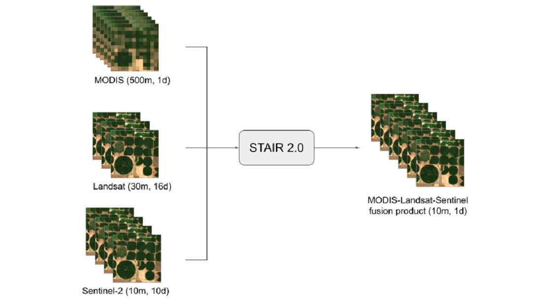
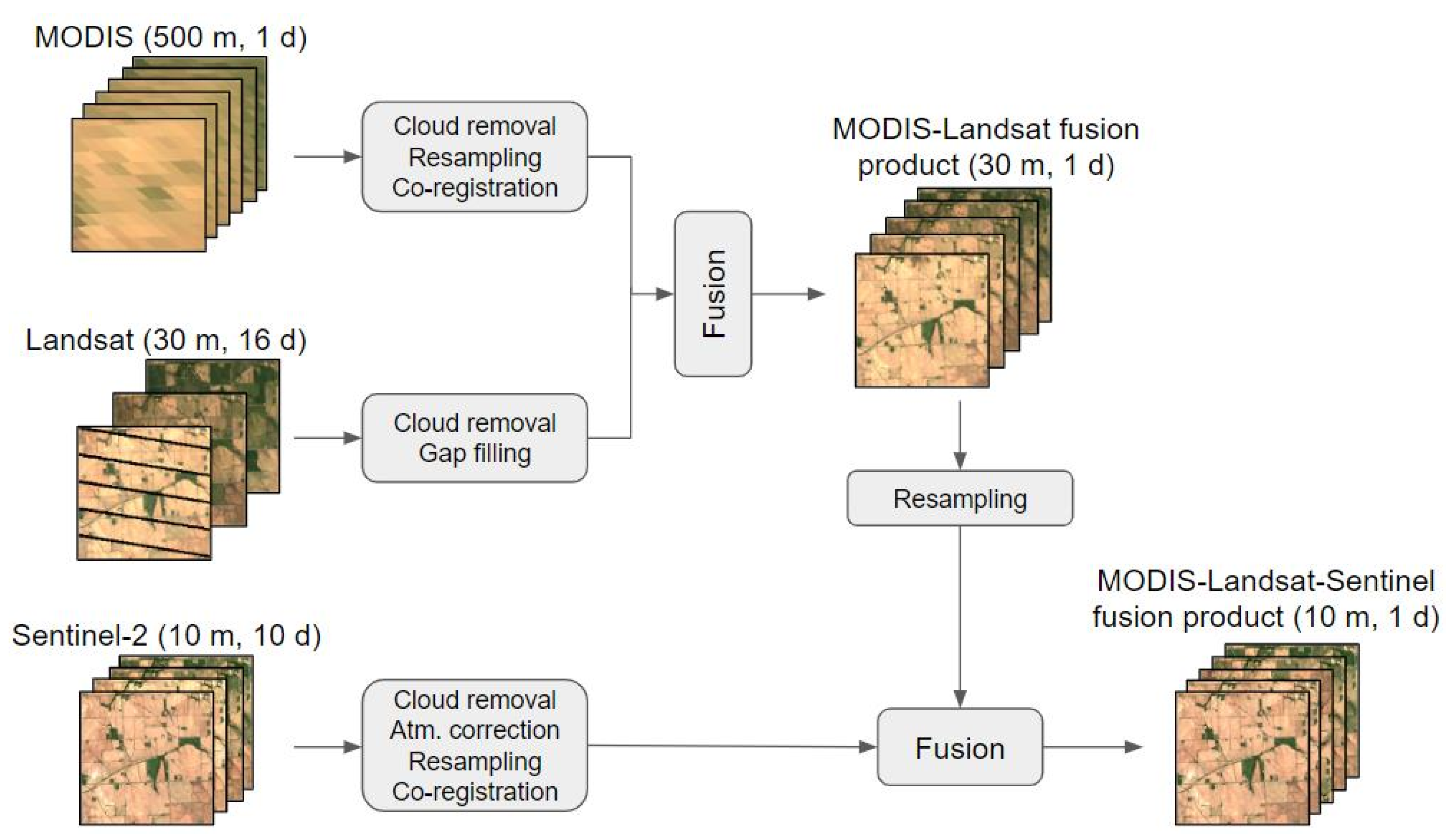
2.4. Fusion of Multiple Sources of Optical Satellite Data

In this section, we describe the fusion framework that fuses multiple sources of optical satellite data (Figure 1). After the imputation of missing pixels for each of the satellite data sources, we used a stepwise strategy to fuse multiple satellite data from coarse resolution to fine resolution. As a proof of concept, we demonstrated how to generate a daily fusion product with 10-m resolution using MODIS (500 m), Landsat (30 m), and Sentinel-2 (10 m) images: we first generated a daily fusion images of 30-m resolution using MODIS and Landsat data, and then fused the Sentinel-2 data and the MODIS–Landsat synthetic data to generate a fusion product of 10-m resolution. Compared to STAIR, STAIR 2.0 provides more informative spatial details in the fusion product by integrating the 10-m-resolution Sentinel-2 dataset (Figure 2). The details of the fusion framework are described below.

2.4.1. Fusion of MODIS and Landsat Data

In the first step, we integrated MODIS and Landsat images to generate a synthetic product with both high spatial resolution (30 m) and high frequency (daily). This synthetic product were later refined to 10-m resolution by fusing with Sentinel-2, which we describe in the next subsection. The fusion method of MODIS and Landsat data was built on our previous algorithm STAIR 1.0. We briefly revisit the method here and refer interested readers to [20] for more details and motivations of the method.

Suppose our goal is to fuse MODIS and Landsat images to generate a time series that has both high spatial resolution and temporal frequency for $n$ dates $t_i$ ($i=1,2,..,n$), and $k$ matching pairs of MODIS and Landsat images (acquired on the same day) are available for dates $T_j$ ($j=1,2,..,k$). After the preprocessing steps, here we assume that the MODIS images have been geo-co-registered and super-sampled to Landsat images such that images from the two datasets have the same size and resolution under the same projection system. The MODIS images are also available for dates $t_i$ ($i=1,2,\dots ,n$) on which we aim to predict the fine-resolution image.

Formally, consider a MODIS image $M$ and a Landsat image $L$ that are both acquired on date $T_j$. We can model the relationship of homogeneous pixels between the Landsat and MODIS images as

$$L\left(x,y,T_j\right)=M\left(x,y,T_j\right)+ϵ(x,y,T_j),$$

(10)

where $L\left(x,y,T_j\right)$ is the surface reflectance value at position $\left(x,y\right)$ in the Landsat image acquired on date $T_j$ and $M\left(x,y,T_j\right)$ has a similar meaning. The term $ϵ(x,y,T_j)$ is the difference between the surface reflectances captured by Landsat and MODIS for $\left(x,y\right)$ at date $T_j$. This difference is often caused by measurement errors of the sensors, solar and viewing angles, systematic noises or biases, and others [18]. Our task is to predict a fine-resolution image $F$ for date $t_p$ where only the MODIS image $M$ is available but the Landsat image is not provided. Using similar notations, we model pixels in the fine-resolution image by $F\left(x,y,t_p\right)=M\left(x,y,t_p\right)+\Delta (x,y,t_p)$, where $\Delta (x,y,t_p)$ is the prediction residuals between the surface reflectances in MODIS image $M$ and the predicted fine-resolution image $F$ of position $\left(x,y\right)$ at date $t_p$. Therefore, one solution of predicting a fine-resolution image $F$ is to first predict the residual term $\Delta$ and then add back the MODIS image $M$. Our method obtains the residues $\Delta (x,y,t_p)$ of position $\left(x,y\right)$ at date $t_i$ by interpolating the surface reflectance differences between the available matching MODIS–Landsat pairs. That is, we first calculate the surface reflectance difference of every position for each date $T_j$ ($j=1,..,k$) as $ϵ(x,y,T_j)=L\left(x,y,T_j\right)-M\left(x,y,T_j\right)$ and then linearly interpolate the difference terms $ϵ(x,y,T_j)$ into each date $t_i$ to obtain the estimated residuals $\Delta (x,y,t_i)$ for all positions $\left(x,y\right)$ on each date $t_i$. Finally, we add the MODIS image back to obtain the fine-resolution predicted image following

$$F\left(x,y,t_i\right)=M\left(x,y,t_i\right)+\Delta (x,y,t_i).$$

(11)

Intuitively, the residuals term $\Delta (x,y,t_i)$ captures the rich spatial information uniquely provided by Landsat for position $\left(x,y\right)$ while the temporal dynamics is encoded in the dense MODIS time series $M\left(x,y,t_i\right)$ for dates $t_i$ ($i=1,2,\dots ,n$). Integrating these two sources of information collectively, the fine-resolution images thus have both rich spatial details and high frequency. We refer to the MODIS–Landsat fusion results as ML-fusion.

2.4.2. Fusion of Sentinel-2 and Synthetic MODIS–Landsat Data

In the last step, we obtain a synthetic MODIS–Landsat product that has daily temporal resolution and 30-m spatial resolution. In this step, we further fuse this product with Sentinel-2 imagery to generate a daily, 10-m fusion product. The fusion process is very similar to the fusion of MODIS and Landsat, except that here Sentinel-2 data are used as the high-resolution image input (10 m) and the synthetic MODIS–Landsat data are the low-resolution image input (30 m). We resample the 30-m synthetic MODIS–Landsat images to 10-m resolution and then estimate the pixel difference $\Delta (x,y,t_i)$ for all positions $\left(x,y\right)$ of the Sentinel 2 image $S\left(x,y,t_i\right)$ and the synthetic MODIS–Landsat image $F\left(x,y,t_i\right)$ at date $t_i$. The final fusion image $P\left(x,y,t_i\right)$ is obtained by computing

$$P\left(x,y,t_i\right)=F\left(x,y,t_i\right)+\Delta (x,y,t_i).$$

(12)

The final fusion product contains daily, 10 m-resolution images. We refer to the MODIS–Landsat–Sentinel-2 fusion results as MLS-fusion.

2.5. Assessments of Fusion Results

To quantitatively assess the fusion results of STAIR 2.0, we held out three observed Sentinel-2 images of Saunders County, NE, on 29 June, 19 July, and 8 August 2017, respectively. These three images were used as the target images and no pixels of target images were available to our fusion method. The availability of Landsat, MODIS, and Sentinel data over this region is visualized in Figure 3. We sampled two areas (with size 3 km × 3 km and 5 km × 5 km, respectively) from each of the withheld images as the test area (Figure S1). The major land cover types for the test areas are corn and soybean. For each test area, we applied STAIR 2.0 on all images for this area in 2017 except the target images to generate a fusion image on that date and compare the fusion image to the observed image.

We calculated two evaluation metrics, the Pearson correlation and the root-mean-square error (RMSE), to quantify how consistent the predicted images and the observed images are in both spatial patterns and surface reflectance values. The Pearson correlation, a number between -1 and +1, measures the consistency of texture features reconstructed by the fusion algorithm and the actual ones in the observed image. A fusion algorithm that accurately recovers the textures in the target image would receive a coefficient close to +1, while an algorithm that poorly captures the textures would receive a smaller or negative coefficient. This RMSE metric quantifies the absolute difference between the predicted and observed surface reflectance values. To explicitly visualize the quality of synthesis, following previous work [32], we calculated the structural similarity (SSIM) for each pixel between the fused image and the observed image. SSIM is a metric between 0 and 1 that quantifies the similarity between two images, with 1 indicating a perfect prediction. We used the scikit-image library (with default parameter) to compute the average SSIM value and generate the SSIM map. For comparison purposes, we include a baseline method where the STAIR 2.0 fusion algorithm was applied to MODIS–Sentinel image pairs. We refer to this baseline method as “MS fusion” while our presented method that integrated MODIS, Landsat, and Sentinel-2 as “MLS fusion” in the following results.

3. Results

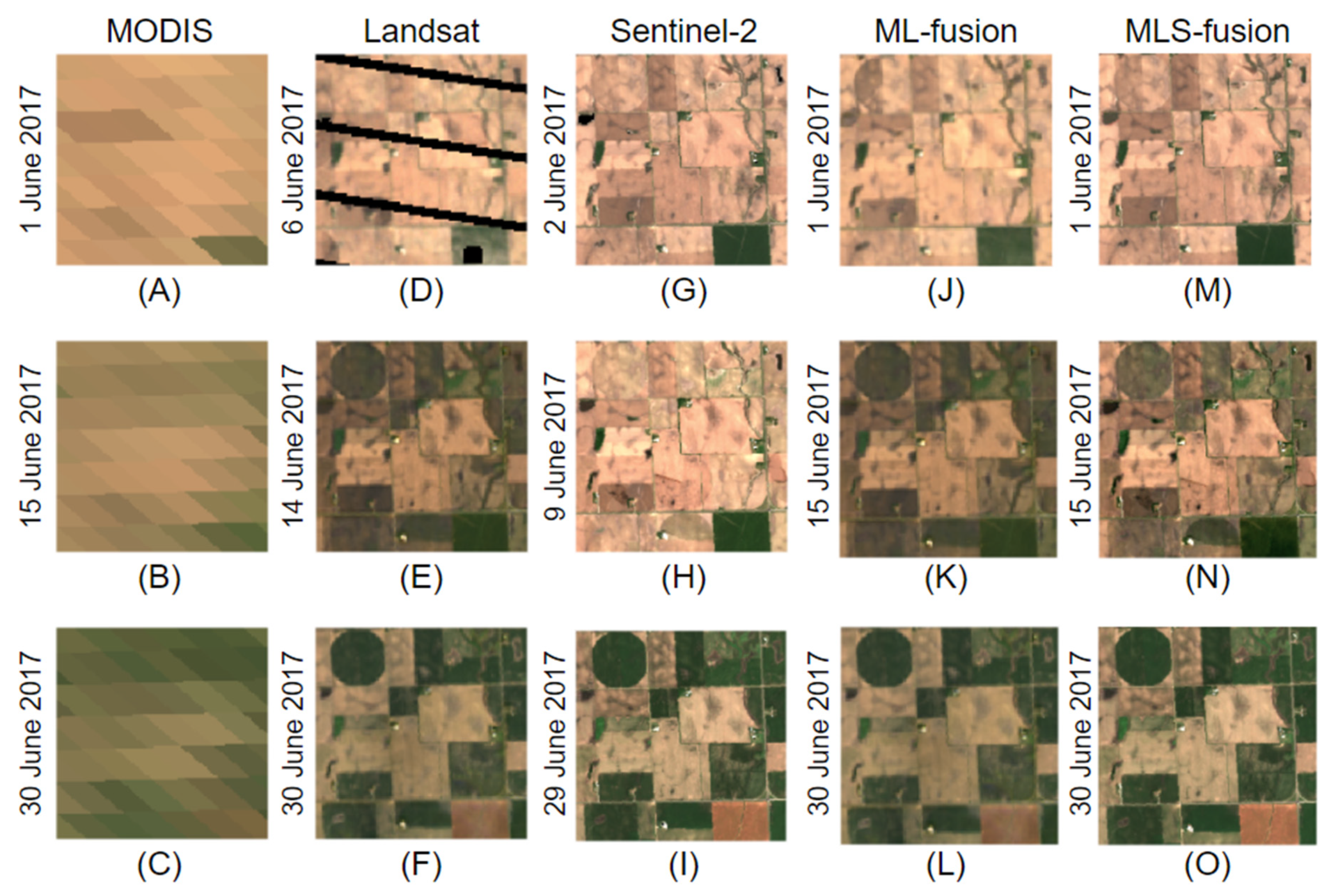
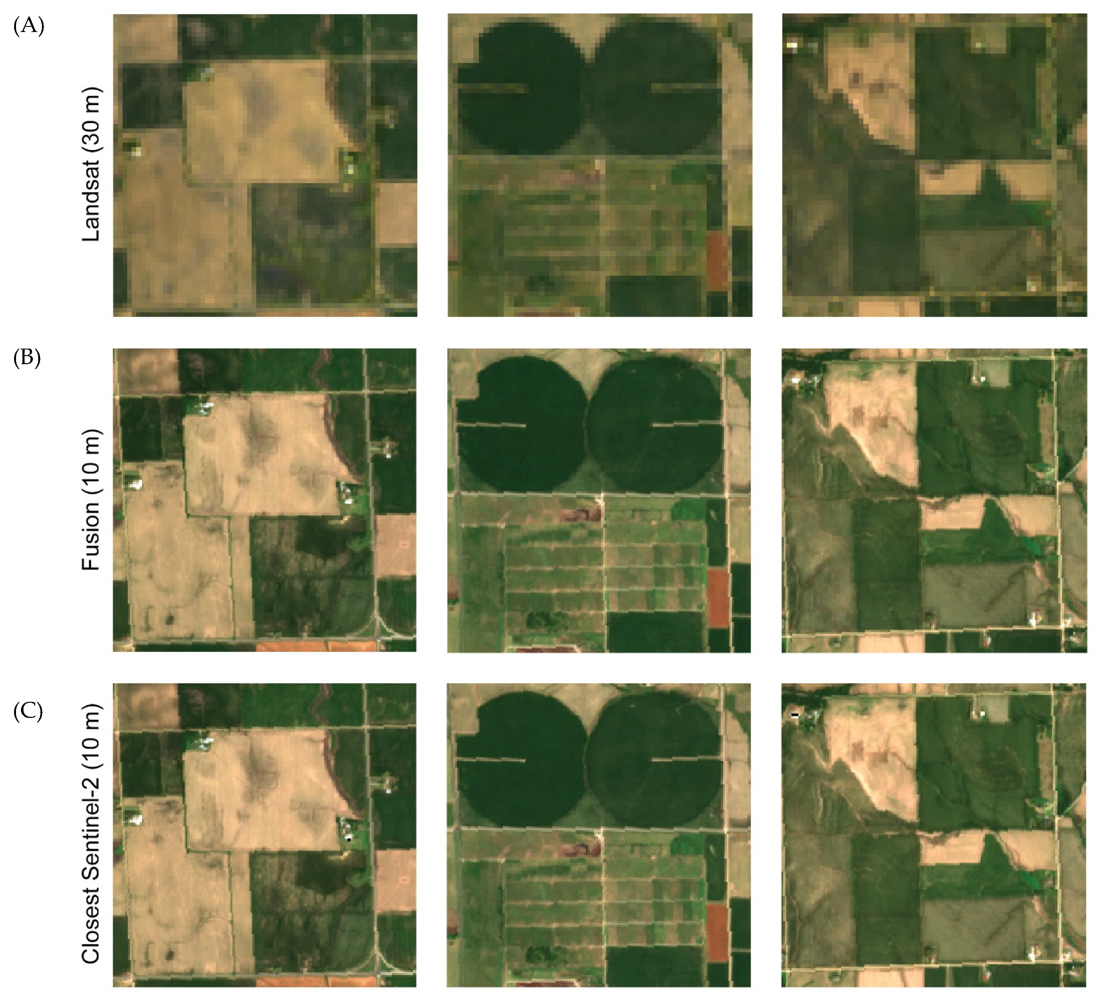
3.1. STAIR 2.0 Generates Daily, 10-m Time Series of Surface Reflectance

We demonstrate the applicability of STAIR 2.0 by applying it to the study area Saunders County, NE in 2017 to produce a fusion product. We compiled MODIS, Landsat and Sentinel-2 images that cover the growing season (1 April 207 to 30 September 2017) and manually removed images with less than 75% clear pixels. In total, 183 MODIS images, 14 Landsat images, and 12 Sentinel-2 images were used in this study. The temporal coverage of the Landsat and Sentinel-2 images is shown in Figure 3.

Taking daily MODIS time series and sparsely available Landsat and Sentinel-2 images (Figure 4A–I) as input, STAIR 2.0 generates a surface reflectance product with both high spatial resolution (10 m) and high temporal resolution (daily). The product contains high-quality time series that covers the growing season (from1 April 207 to 30 September 2017). Images in the time-series product are cloud-/gap-free. Missing-value pixels that are due to Landsat 7 un-scanned strips or clouds (e.g., Figure 4D) were filled accurately and effectively by the imputation process. Using a stepwise fusion strategy, STAIR 2.0 first combines the MODIS and Landsat datasets to generate an intermediate fusion product that contains daily, 30 m-resolution time series (Figure 4J–L). This MODIS–Landsat fusion product is then upsampled to 10-m resolution and fused with the Sentinel-2 dataset, resulting in a fusion product that contains a time series cloud-/gap-free images with 10-m resolution and daily frequency (Figure 4M–O).

The dense time series produced by STAIR 2.0 also enables the high-resolution monitoring of the land surface. For example, for 30 June 2017, where there was one Landsat acquisition for Saunders, NE while no Sentinel-2 image was available, we applied STAIR 2.0 to generate a synthetic 10-m resolution image (Figure 5). Compared to the available Landsat image, the fusion image provides richer spatial information about the land surfaces and reveals many nuanced details that were not captured by Landsat due to the limitation of sensor resolution. In the next section, we quantitatively show that STAIR 2.0 not only refines the spatial details of land surfaces but also accurately recovers the time series of surface reflectance. Taken together, the STAIR 2.0 algorithm has great potential in enabling a more precise and fine-scale monitoring and analysis of the dynamics of land surfaces.

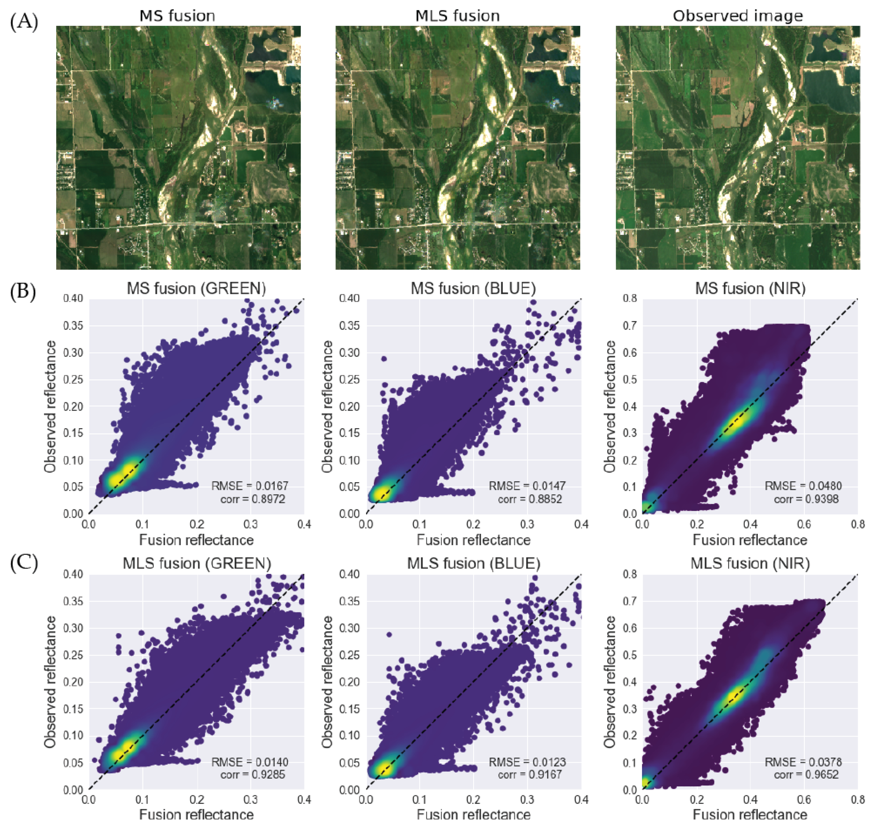
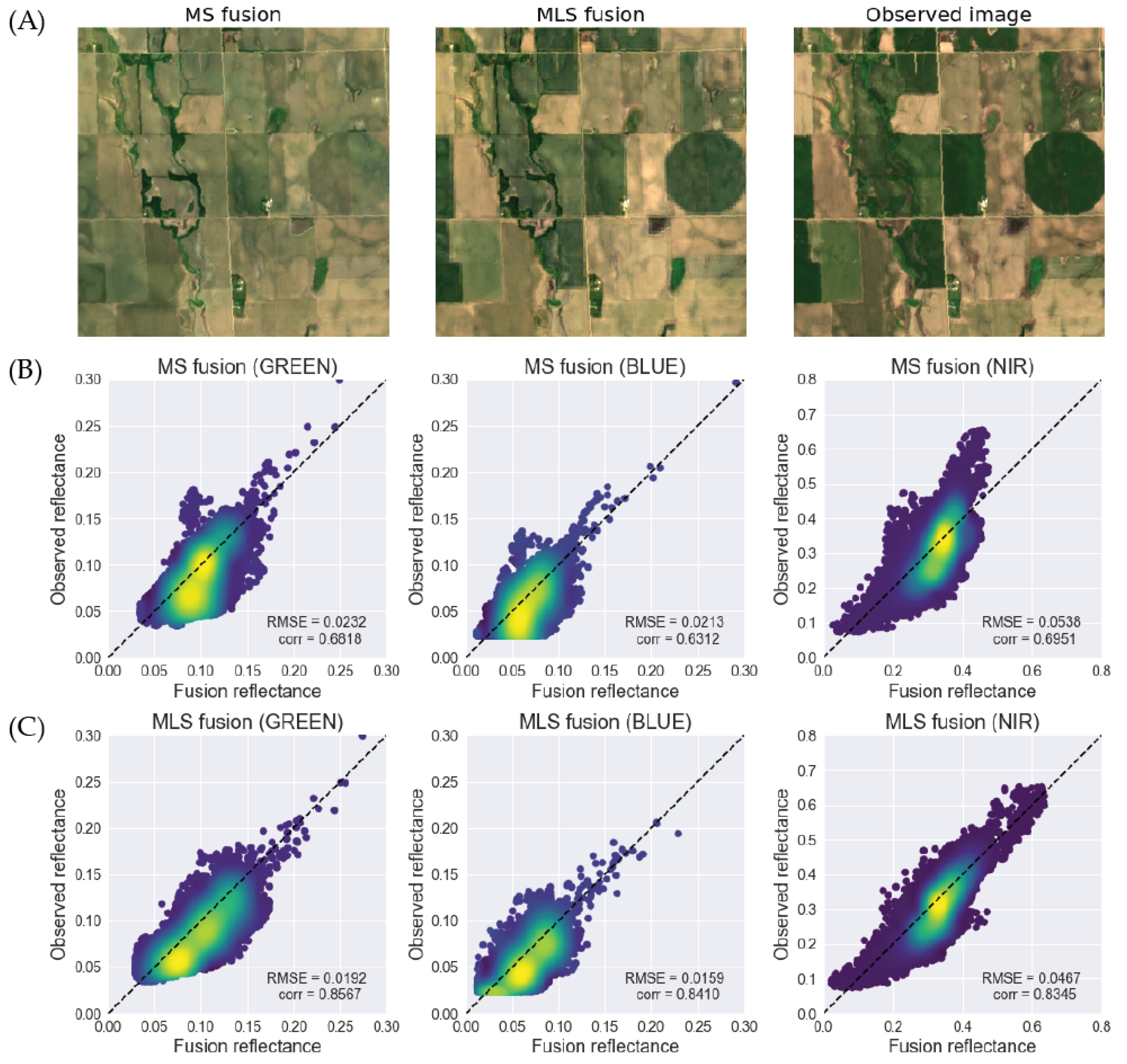
3.2. Quantitative Assessments

By evaluating STAIR 2.0 on the withheld test areas, we found that STAIR 2.0 produces accurate fusion results with an RMSE <0.1, a correlation around 0.8-0.9, and an SSIM >0.9 for red, NIR, and SWIR2 bands on all of the test areas (

Table 2. Quantitative assessments of STAIR 2.0 fusion. Three observed Sentinel-2 images on 29 June, July 19, and 8 August 2017 were held out as the ground truth image to assess the fusion results of STAIR 2.0. For each image, two areas were randomly sampled as the test areas. Two fusion settings, MODIS–Sentinel (MS) and MODIS–Landsat–Sentinel (MLS), were compared. Pearson correlation, root-mean-square error (RMSE), and structural similarity (SSIM) were used as the evaluation metrics. Results of red, NIR, and SWIR2 bands are shown. For each test band, the better performance (lower RMSE, higher correlation, or higher SSIM) is in bold. See Table S1 for the results of other bands (green, blue, and SWIR1).

Test Date	Band	RMSE		Pearson correlation		SSIM
		MS Fusion	MLS Fusion	MS Fusion	MLS Fusion	MS Fusion	MLS Fusion
29 June 2017 (area 1)	Red	0.0354	0.0222	0.7409	0.9117	0.8667	0.9349
	NIR	0.0656	0.0620	0.5570	0.7509	0.8767	0.9002
	SWIR2	0.0558	0.0455	0.7863	0.9341	0.8836	0.9232
29 June 2017 (area 2)	Red	0.0334	0.0236	0.7023	0.9042	0.884	0.9342
	NIR	0.0538	0.0467	0.6951	0.8345	0.898	0.9222
	SWIR2	0.0563	0.0693	0.7669	0.8800	0.8903	0.9002
19 July 2017 (area 1)	Red	0.0195	0.0165	0.6770	0.7675	0.9328	0.9522
	NIR	0.0529	0.0458	0.7656	0.8617	0.9108	0.9249
	SWIR2	0.0315	0.0336	0.8123	0.8184	0.9513	0.9490
19 July 2017 (area 2)	Red	0.0216	0.0181	0.9035	0.9344	0.949	0.9595
	NIR	0.0515	0.0380	0.9376	0.9669	0.9131	0.9142
	SWIR2	0.0339	0.0248	0.9060	0.9494	0.9467	0.9539
8 August 2017 (area 1)	Red	0.0103	0.0100	0.8328	0.8508	0.9785	0.9813
	NIR	0.0497	0.0432	0.9059	0.9300	0.9274	0.9344
	SWIR2	0.0185	0.0180	0.8701	0.8762	0.9771	0.9782
8 August 2017 (area 2)	Red	0.0109	0.0096	0.8485	0.8877	0.9745	0.9797
	NIR	0.0417	0.0347	0.9427	0.9564	0.9288	0.9361
	SWIR2	0.0144	0.0134	0.9337	0.9422	0.9817	0.9818

). These results suggest that STAIR 2.0 is able to both capture the spatial texture patterns and accurately predict the surface reflectance values. In addition, STAIR 2.0 under the MLS fusion setting consistently outperforms the MS fusion setting in terms of Pearson correlation, RMSE, and SSIM. The difference between these two settings is that STAIR 2.0 further integrates Landsat in the MLS fusion setting but not in the MS setting. We also observed similar results for other bands, including green, blue, and SWIR1 bands (see Table S1 for detailed results). We visualize one example of the STAIR 2.0 fusion image for both MS and MLS fusion settings in Figure 6. The qualitative comparison reveals that the MLS fusion image is more consistent with the observed image in color scheme and provides more accurate texture details. This was also confirmed by the quantitative evaluation, where the MLS fusion achieved higher correlation and lower RMSE than the MS fusion (Figure 6). For example, for the NIR band, the RMSE and correlation of the MLS fusion are 0.037 and 0.965, which outperforms the MS fusion (with RMSE 0.048 and correlation 0.939). To further assess the fusion quality, we calculated the SSIM values for both MS and MLS fusion results. MLS fusion improved the SSIM value from 0.943 to 0.956 as compared to MS fusion (Table S1). We visualized the SSIM maps to show the pixel-level SSIM values in Figure S2, which clearly shows that MLS fusion captures more details accurately then MS fusion. These results thus indicate that multiple sources of optical satellite data can mitigate the sparsity in the data and improve the accuracy of the fusion images.

3.3. Values of Integrating Three Satellite Sources

To demonstrate the advantages of integrating more types of satellite data for fusion, we performed a case study in which we held out one Sentinel-2 image on June 29 (DOY 180) and applied STAIR 2.0 to generate a fusion image for this target date. The removal of this image makes the data availability around this date very sparse (Figure 3) and the temporarily closest Sentinel-2 images are 20 days apart (on DOY 160 and DOY 200), creating a challenging setting for evaluating the fusion algorithm. The sparsity of the Sentinel-2 time series in this timeframe makes the fusion a challenging task as there is little accurate information about the target date available for the fusion algorithm. Moreover, the surface reflectance typically changes rapidly in a nonlinear way in this timeframe, which further exacerbates the data sparsity issue.

We first applied STAIR 2.0 to generate the MODIS–Sentinel-2 fusion images (MS fusion) for the target date. The fusion image does not fully capture the texture details or accurately recover the surface reflectance (Figure 7A). The RGB visualization of the fusion image is also clearly different from the observed image (Figure 7A). The reason is mainly the sparse frequency of Sentinel-2 data and the low spatial resolution of MODIS data: the surface reflectance greatly changes in this timeframe and the closest available Sentinel-2 images, which are 20 days apart, cannot offer accurate reference reflectance values for the target date. The MODIS data, even though at a daily frequency, have a relatively low spatial resolution and did not provide informative details or effective correction of reflectance values in the fusion. We note that existing fusion algorithms that integrate two types of satellite data (e.g., STARFM and ESTARFM) would also have the same issue here due to a similar reason.

Next, we applied STAIR 2.0 to further integrate Landsat (MLS fusion), in addition to MODIS and Sentinel-2, to produce a fusion image for the target date. The Landsat dataset provides additional information to the input time series. For example, there are four Landsat images (on DOYs 165, 181, 189, and 197) that are closer to the target date than the two temporarily closest Sentinel-2 images, and one of them is only one day away from the target date. We observed that introducing the Landsat effectively mitigated the data sparsity issue. The MLS fusion image is visually more consistent with the observed image than the MS fusion image (Figure 7B). The quantitative evaluation also indicates that the MLS fusion image has lower RMSE error and higher correlation than the MS fusion image across three bands (Figure 7C). Although the MLS fusion image still does not fully recover texture details and surface reflectance, we expect the fusion results can be improved qualitatively and quantitatively providing more available Landsat and/or Sentinel-2 images in the input time series.

We further demonstrated the utility of MLS fusion by using the fusion data to derive the normalized difference vegetation index (NDVI) for land covers. We selected a region (Figure S3) of Saunders, NE, in 2017 and used the MS and MLS fusion data to compute the NDVI series. We observed that the fusion data captured the temporal dynamics of the NDVI time series (Figure S3). By integrating more sources of data, the MLS fusion, as compared to the MS fusion, reflects more detailed temporal changes in the time series.

Low coverage on the temporal dimension is a frequent issue in the spatial-temporal fusion of optical satellites, due to various reasons including cloud contamination and the satellite revisit frequency. The above results demonstrate that integrating multiple satellite sources can effectively mitigate this issue. With its ability to fuse multiple sources of satellite data, we expect STAIR 2.0 to be a practically useful fusion algorithm that can fully take advantage of each input dataset to generate a high-quality product of surface reflectance time series.

4. Discussion

4.1. Advancements of STAIR 2.0

Compared to its predecessor STAIR, STAIR 2.0 achieves several improvements. It fuses more satellite datasets, with higher computational efficiency, to generate a surface reflectance product at a higher resolution. The synthetic product consists of daily, could-/gap-free, spectral-/spatial- co-registered surface reflectance observations at 10-m resolution.

STAIR 2.0 offers the flexibility and convenience of usage for fusing multiple satellite sources. STAIR 2.0 is able to integrate the time series of input satellite data that consist of a large number of images, fully taking advantage of complementary information available across different data. In contrast, fusion methods such as STARFM and ESTARFM only support up to two matching Landsat–MODIS image pairs as input and thus have limited integration ability. In addition, STAIR 2.0 does not require the input to contain MODIS–Landsat–Sentinel triples that are nearly coincident: it first fuses MODIS and Landsat data to generate daily fusion images so each Sentinel-2 image will have a matching fusion image. This is a big relaxation of stringent requirements in previous fusion methods that integrate three types of satellite data. For example, the CESTEM method must have near-coincident MODIS–Landsat–PlanetScope images as input, which greatly limits its applicability when coincident images are very scarce [22].

STAIR 2.0 also provides a high-performance gap-filling algorithm to impute missing-value pixels due to cloud or sensor damage in input images. Fusion methods such as STARFM and ESTARFM do not explicitly impute missing-value pixels in input pixels, e.g., cloud regions or strips in Landsat 7 SLC-off images. Instead, these methods rely on users to provide cloud-/gap-free input images. To deal with this, users have to apply other cloud detection and gap-filling algorithms before applying these fusion methods. STAIR 2.0 streamlines this process by developing a fusion framework with the gap-filling function, which frees users from the tedious process of combining multiple independently developed methods into a pipeline. Our gap-filling algorithm is an improved version of the one in STAIR and is itself a novel method. It additionally uses temporal surface reflectance profiles to search similar neighborhood pixels to better adjust a filled pixel, thus leading to higher-quality gap-filling results. The gap-filling algorithm is also optimized to run on multiple CPU cores. When applied to the test areas in this work, the multi-core version of STAIR 2.0 is 20× faster than its single-core version. Different from existing gap-filling algorithms (e.g., NSPI [33] and its enhanced version GNSPI [34]), which use a single reference image for imputing missing-value pixels, our gap-filling algorithm uses a time series of reference images and thus is more effective in identifying similar pixels and producing high-fidelity filling results. In addition to facilitating the downstream fusion process, the gap-filling algorithm is also of independent interest and useful in other remote sensing-based analyses.

4.2. Spectral Correction and Spatial Alignments of Multiple Satellite Sources

Images from different satellite sensors have many differences in spatial resolution, bandwidth, spectral response, solar geometry, and viewing angle. Therefore, for the best practice, cautions should be given before fusing different satellite data sources. Major considerations include unifying spectral responses and cross geo-registration. Firstly, differences in bandwidth, spectral response, and atmospheric conditions may lead to systematic bias across different types of satellite images. Most existing fusion methods, such as STARFM, have already taken the systematic bias into account in modeling the relationship between Landsat and MODIS surface reflectance. STAIR implicitly considers the differences in spectral responses of Landsat and MODIS and thus has a limited impact on fusion accuracy. In STAIR 2.0, we additionally performed pre-processing using calibrated models from literature to unify the spectral responses across bands and sensors. Therefore, the spectral difference does not have a significant impact on fusion accuracy in most spatiotemporal fusion methods. On the other hand, cross-sensor geo-registration is a critical factor for the successful fusion of multiple satellite sources. Virtually all spatiotemporal fusion methods, including STARFM and STAIR 2.0, assume that a coarse-resolution pixel and all of its corresponding internal fine-resolution pixels observe the same region of the land surface. However, satellite sensors have their own inherent uncertainty of geolocations, and geolocation errors exist across different sensors, all of which will lead to misalignment of geolocations in images from different satellite sensors. The issue becomes more notable for the fusion of two high-resolution satellite data. For example, it has been reported that the current Landsat and Sentinel-2 images are misaligned by more than several 10-m pixels [35]. In STAIR 2.0, we used a tie-point matching approach to perform the geo-registration of different satellite data sources. Other approaches, for example, based on image texture/spectral matching algorithms [35], are alternative solutions to our approach.

4.3. Fusion Strategy of Multiple Satellite Sources

To date, there are very few efforts on the spatiotemporal fusion of more than three satellite data sources, and there is no consensus strategy for fusing multiple sources, i.e., in which order and in what manner should multiple (more than three) datasets be integrated. For example, in CESTEM, PlanetScope images are compared to MODIS and Landsat images separately for calibration purposes, the PlanetScope images are integrated with Landsat images to produce high-frequency Landsat-consistent PlanetScope images. In STAIR 2.0, we used a simple yet effective stepwise approach to integrate MODIS, Landsat, and Sentinel-2 images. MODIS (500 m) and Landsat (30 m) images are first fused to generate daily synthetic images (30 m), which are then further fused with Sentinel-2 images (10 m) to produce a final fusion product with daily frequency and 30-m resolution. There are other different fusion strategies to integrate the three datasets. For example, one can first down-scale the Sentinel-2 images to the resolution of Landsat and generate a Landsat–Sentinel time series, then apply the fusion on MODIS and this hybrid time series. Since the information is denser in the hybrid time series, this fusion strategy potentially will improve fusion accuracy. It should be noted that spectral correction and spatial alignment are critical in constructing the hybrid time series from two- or multiple-source satellite data. Moreover, benchmarking different fusion strategies for the data from the three satellites could be a valuable future direction of the development of spatiotemporal fusion methods.

4.4. Computational Efficiency and Scalability

Spatiotemporal fusion methods with high computational efficiency are extremely needed in high-resolution monitoring and modeling of land surface dynamics, especially for continental-scale applications. The major bottleneck of efficiency in STAIR 2.0 is the extensive computation of pairwise similarity of pixels within a sliding window. Pixel-wise computation and moving window strategy are also identified as the major factors that limit the wide application of existing spatiotemporal fusion methods such as STARFM [19]. To boost the fusion process, we implemented a multi-process version of STAIR 2.0 that performs the pairwise similarity calculation for multiple sliding windows in parallel on multiple CPU cores. We found this optimization brings a 20X speedup for the fusion of Champaign, Illinois, USA, 2017, using 20 CPU cores. There is still room for efficiency improvement of STAIR 2.0. For example, the current framework is implemented in Python and utilizes CPUs only. Orders of magnitude of acceleration for the whole fusion pipeline can be achieved by translating the implementation from Python to C/C++ and parallelizing it on GPUs.

5. Conclusions

In this paper, we present STAIR 2.0, a generic and automatic fusion method to integrate multiple satellite data sources, including MODIS, Landsat, and Sentinel-2, to generate daily, 10-m resolution, cloud- and gap-free time series of surface reflectance. STAIR 2.0 is an improved and extended version of STAIR, a fusion method we developed to integrate MODIS and Landsat data to produce a daily, 30 m surface reflectance product. STAIR 2.0 consists of an effective gap-filling algorithm and a flexible fusion method. Compared to its predecessor, STAIR 2.0 provides an improved gap-filling algorithm that more effectively imputes the missing-value pixels in the input image due to cloud or sensor damage, as well as a flexible fusion framework that uses a stepwise strategy to integrate MODIS, Landsat, and Sentinel-2 data. The gap-filling algorithm, equipped with a multiprocessing implementation, efficiently utilizes time series similarity to impute missing-value pixels due to cloud or sensor damage in the input image. The fusion method integrates the three satellite sources using a stepwise strategy, from coarse resolution (MODIS) to fine resolution (Sentinel-2). This work is a demonstration of the STAIR algorithm’s nature of genericness and flexibility to fuse all sorts of optical satellite data after the proper pre-processing. Through quantitative assessments, we show that STAIR 2.0 is able to produce accurate fusion products, with a low RMSE and a high correlation as compared to the ground truth images. We also demonstrate that the fusion of three satellite sources, by leveraging the information from more frequently dynamics and finer spatial scales, provides independent and additive values that cannot be offered by the integration of only two satellite sources. We expect STAIR 2.0 to be a practical tool for various remote sensing applications based on time series modeling.

References

1. Schneider, A. Monitoring land cover change in urban and peri-urban areas using dense time stacks of Landsat satellite data and a data mining approach. Remote Sens. Environ. 2012, 124, 689–704. [Google Scholar] [CrossRef]
2. Cai, Y.; Guan, K.; Peng, J.; Wang, S.; Seifert, C.; Wardlow, B.; Li, Z. A high-performance and in-season classification system of field-level crop types using time-series Landsat data and a machine learning approach. Remote Sens. Environ. 2018, 210, 35–47. [Google Scholar] [CrossRef]
3. Gao, F.; Anderson, M.C.; Zhang, X.; Yang, Z.; Alfieri, J.G.; Kustas, W.P.; Mueller, R.; Johnson, D.M.; Prueger, J.H. Toward mapping crop progress at field scales through fusion of Landsat and MODIS imagery. Remote Sens. Environ. 2017, 188, 9–25. [Google Scholar] [CrossRef] [Green Version]
4. Johnson, M.D.; Hsieh, W.W.; Cannon, A.J.; Davidson, A.; Bédard, F. Crop yield forecasting on the Canadian Prairies by remotely sensed vegetation indices and machine learning methods. Agric. For. Meteorol. 2016, 218, 74–84. [Google Scholar] [CrossRef]
5. Guan, K.; Wu, J.; Kimball, J.S.; Anderson, M.C.; Frolking, S.; Li, B.; Hain, C.R.; Lobell, D.B. The shared and unique values of optical, fluorescence, thermal and microwave satellite data for estimating large-scale crop yields. Remote Sens. Environ. 2017, 199, 333–349. [Google Scholar] [CrossRef] [Green Version]
6. Guan, K.; Li, Z.; Rao, L.N.; Gao, F.; Xie, D.; Hien, N.T.; Zeng, Z. Mapping Paddy Rice Area and Yields Over Thai Binh Province in Viet Nam from MODIS, Landsat, and ALOS-2/PALSAR-2. IEEE J. Sel. Top. Appl. Earth Obs. Remote Sens. 2018, 11, 2238–2252. [Google Scholar] [CrossRef]
7. Jamshidi, S.; Zand-Parsa, S.; Naghdyzadegan Jahromi, M.; Niyogi, D. Application of a simple Landsat-MODIS fusion model to estimate evapotranspiration over a heterogeneous sparse vegetation region. Remote Sens. 2019, 11, 741. [Google Scholar] [CrossRef] [Green Version]
8. Jamshidi, S.; Zand-parsa, S.; Pakparvar, M.; Niyogi, D. Evaluation of evapotranspiration over a semiarid region using multiresolution data sources. J. Hydrometeorol. 2019, 20, 947–964. [Google Scholar] [CrossRef]
9. Stone, B., Jr.; Rodgers, M.O. Urban form and thermal efficiency: How the design of cities influences the urban heat island effect. Am. Plan. Assoc. J. Am. Plan. Assoc. 2001, 67, 186. [Google Scholar] [CrossRef]
10. Imhoff, M.L.; Zhang, P.; Wolfe, R.E.; Bounoua, L. Remote sensing of the urban heat island effect across biomes in the continental USA. Remote Sens. Environ. 2010, 114, 504–513. [Google Scholar] [CrossRef] [Green Version]
11. Streets, D.G.; Canty, T.; Carmichael, G.R.; De Foy, B.; Dickerson, R.R.; Duncan, B.N.; Edwards, D.P.; Haynes, J.A.; Henze, D.K.; Houyoux, M.R.; et al. Emissions estimation from satellite retrievals: A review of current capability. Atmos. Environ. 2013, 77, 1011–1042. [Google Scholar] [CrossRef] [Green Version]
12. Arvidson, T.; Goward, S.; Gasch, J.; Williams, D. Landsat-7 long-term acquisition plan. Photogramm. Eng. Remote Sens. 2006, 72, 1137–1146. [Google Scholar] [CrossRef]
13. Budaev, D.; Lada, A.; Simonova, E.; Skobelev, P.; Travin, V.; Yalovenko, O. Conceptual design of smart farming solution for precise agriculture. Manag. App. Complex Syst. 2019, 13, 309–316. [Google Scholar]
14. Dong, T.; Shang, J.; Liu, J.; Qian, B.; Jing, Q.; Ma, B.; Huffman, T.; Geng, X.; Sow, A.; Shi, Y.; et al. Using RapidEye imagery to identify within-field variability of crop growth and yield in Ontario, Canada. Precis. Agric. 2019, 20, 1231–1250. [Google Scholar] [CrossRef]
15. Cammalleri, C.; Anderson, M.C.; Gao, F.; Hain, C.R.; Kustas, W.P. A data fusion approach for mapping daily evapotranspiration at field scale. Water Resour. Res. 2013, 49, 4672–4686. [Google Scholar] [CrossRef]
16. Wu, M.; Wu, C.; Huang, W.; Niu, Z.; Wang, C.; Li, W.; Hao, P. An improved high spatial and temporal data fusion approach for combining Landsat and MODIS data to generate daily synthetic Landsat imagery. Inf. Fusion 2016, 31, 14–25. [Google Scholar] [CrossRef]
17. Gao, F.; Masek, J.; Schwaller, M.; Hall, F. On the blending of the Landsat and MODIS surface reflectance: Predicting daily Landsat surface reflectance. IEEE Trans. Geosci. Remote Sens. 2006, 44, 2207–2218. [Google Scholar]
18. Zhu, X.; Chen, J.; Gao, F.; Chen, X.; Masek, J.G. An enhanced spatial and temporal adaptive reflectance fusion model for complex heterogeneous regions. Remote Sens. Environ. 2010, 114, 2610–2623. [Google Scholar] [CrossRef]
19. Zhu, X.; Cai, F.; Tian, J.; Williams, T. Spatiotemporal fusion of multisource remote sensing data: Literature survey, taxonomy, principles, applications, and future directions. Remote Sens. 2018, 10, 527. [Google Scholar]
20. Luo, Y.; Guan, K.; Peng, J. STAIR: A generic and fully-automated method to fuse multiple sources of optical satellite data to generate a high-resolution, daily and cloud-/gap-free surface reflectance product. Remote Sens. Environ. 2018, 214, 87–99. [Google Scholar] [CrossRef]
21. Claverie, M.; Ju, J.; Masek, J.G.; Dungan, J.L.; Vermote, E.F.; Roger, J.-C.; Skakun, S.; Justice, C. The Harmonized Landsat and Sentinel-2 surface reflectance data set. Remote Sens. Environ. 2018, 219, 145–161. [Google Scholar] [CrossRef]
22. Houborg, R.; McCabe, M.F. A CubeSat enabled spatio-temporal enhancement method (CESTEM) utilizing Planet, Landsat and MODIS data. Remote Sens. Environ. 2018, 209, 211–226. [Google Scholar] [CrossRef]
23. Schaaf, C.; Gao, F.; Strahler, A.H.; Lucht, W.; Li, X.; Tsang, T.; Strugnell, N.C.; Zhang, X.; Jin, Y.; Muller, J.-P.; et al. First operational BRDF, albedo nadir reflectance products from MODIS. Remote Sens. Environ. 2002, 83, 135–148. [Google Scholar] [CrossRef] [Green Version]
24. Wang, Z.; Schaaf, C.; Strahler, A.H.; Chopping, M.J.; Román, M.O.; Shuai, Y.; Woodcock, C.E.; Hollinger, D.Y.; Fitzjarrald, D.R. Evaluation of MODIS albedo product (MCD43A) over grassland, agriculture and forest surface types during dormant and snow-covered periods. Remote Sens. Environ. 2014, 140, 60–77. [Google Scholar] [CrossRef] [Green Version]
25. Masek, J.; Vermote, E.; Saleous, N.; Wolfe, R.; Hall, F.; Huemmrich, K.; Lim, T. A Landsat Surface Reflectance Dataset for North America, 1990–2000. IEEE Geosci. Remote Sens. Lett. 2006, 3, 68–72. [Google Scholar] [CrossRef]
26. Roy, D.; Wulder, M.A.; Loveland, T.; Woodcock, C.E.; Allen, R.; Anderson, M.C.; Helder, D.; Irons, J.; Johnson, D.; Kennedy, R.; et al. Landsat-8: Science and product vision for terrestrial global change research. Remote Sens. Environ. 2014, 145, 154–172. [Google Scholar] [CrossRef] [Green Version]
27. Louis, J.; Debaecker, V.; Pflug, B.; Main-Knorn, M.; Bieniarz, J.; Mueller-Wilm, U.; Cadau, E.; Gascon, F. Sentinel-2 Sen2Cor: L2A Processor for Users. In Proceedings of the Living Planet Symposium 2016, Prague, Czech Republic, 9–13 May 2016; Volume 740, p. 91. [Google Scholar]
28. Lowe, D. Object Recognition from Local Scale-Invariant Features. In Proceedings of the Seventh IEEE International Conference on Computer Vision, Corfu, Greece, 20–27 September 1999. [Google Scholar]
29. Roy, D.P.; Kovalskyy, V.; Zhang, H.K.; Vermote, E.F.; Yan, L.; Kumar, S.S.; Egorov, A. Characterization of Landsat-7 to Landsat-8 reflective wavelength and normalized difference vegetation index continuity. Remote Sens. Environ. 2016, 185, 57–70. [Google Scholar] [CrossRef] [Green Version]
30. Lloyd, S. Least squares quantization in PCM. IEEE Trans. Inf. Theory 1982, 28, 129–137. [Google Scholar] [CrossRef]
31. Tibshirani, R.; Walther, G.; Hastie, T. Estimating the number of clusters in a data set via the gap statistic. J. R. Stat. Soc. Ser. B (Stat. Methodol.) 2001, 63, 411–423. [Google Scholar] [CrossRef]
32. Zhu, X.; Helmer, E.H.; Gao, F.; Liu, D.; Chen, J.; Lefsky, M.A. A flexible spatiotemporal method for fusing satellite images with different resolutions. Remote Sens. Environ. 2016, 172, 165–177. [Google Scholar] [CrossRef]
33. Chen, J.; Zhu, X.; Vogelmann, J.E.; Gao, F.; Jin, S. A simple and effective method for filling gaps in Landsat ETM+ SLC-off images. Remote Sens. Environ. 2011, 115, 1053–1064. [Google Scholar] [CrossRef]
34. Zhu, X.; Liu, D.; Chen, J. A new geostatistical approach for filling gaps in Landsat ETM+ SLC-off images. Remote Sens. Environ. 2012, 124, 49–60. [Google Scholar] [CrossRef]
35. Yan, L.; Roy, D.; Zhang, H.; Li, J.; Huang, H. An automated approach for sub-pixel registration of Landsat-8 Operational Land Imager (OLI) and Sentinel-2 Multi Spectral Instrument (MSI) imagery. Remote Sens. 2016, 8, 520. [Google Scholar] [CrossRef] [Green Version]
Figure 1. Schematic overview of the fusion method of STAIR 2.0. STAIR 2.0 is a generic framework that can fuse multiple sources of optical satellite data and produce a high-resolution, daily and cloud-/gap-free surface reflectance product. The input of STAIR 2.0 is multiple sources of optical satellite data with different spatial and temporal resolutions, i.e., MODIS (500 m, 1 day), Landsat (30 m, 16 days), and Sentinel-2 (10–20 m, 10 days). STAIR 2.0 pre-processes the input data, imputes missing-value pixels (due to cloud and sensor damages), and uses a stepwise strategy—from coarse resolution to fine resolution—to produce a high spatial- (10m) and temporal-resolution (daily) product.
Remotesensing 12 03209 g001
Figure 2. Example visualization of MODIS, Landsat, and Sentinel-2 images: (A) three temporarily close images of MODIS (June 30, 2017), Landsat (June 30, 2017), and Sentinel-2 (June 29, 2017) dataset are selected and the RGB composite images are displayed for a sub-region of Saunders, NE; and (B,C) two levels of zoom-in views of the selected region.
Remotesensing 12 03209 g002
Figure 3. Data availability of Landsat and Sentinel-2 imaginary. Each dot represents an acquisition of Landsat or Sentinel-2 image from April 1 to September 30, 2017, in Saunders, NE. The x-axis shows the DOY (day of the year) from April 1 (DOY 91) to September 30 (DOY 273). Images with clear pixels less than 75% were removed and not shown.
Remotesensing 12 03209 g003
Figure 4. Example of STAIR 2.0 fusion results. STAIR 2.0 is applied to produce the daily time-series with 10-m resolution that covers the growing season (from 1 April to 30 September 2017) of a test region in Saunders, NE in 2017. The input and fused images in June 2017 are shown. (A–C) MODIS images are available every day and three MODIS images on (A) 1 June 2017, (B) 15 June 2017, and (C) 30 June 2017are shown. (D–F) Three Landsat images are available, on (D) 6 June 2017, (E) 14 June 2017, and (F) 30 June 2017. (G–I) Three Sentinel-2 images are available, on (G) 2 June 2017, (H) 9 June 2017, and (I) 29 June 2017. (J–L) intermediate MODIS–Landsat fusion product (ML-fusion). MODIS and Landsat datasets are fused to generate a daily, 30-m fusion product. Three ML-fusion images on (J) 1 June 2017, (K) 15 June 2017, and (L) 30 June 2017 are shown. (M–O) final MODIS–Landsat–Sentinel-2 fusion product (MLS-fusion). Three MLS images on (M) 1 June 2017, (N) 15 June 2017, and (O) 30 June 2017 are shown. Missing-value pixels due to clouds or Landsat 7 un-scanned strips are shown as black pixels.
Remotesensing 12 03209 g004
Figure 5. Comparison of the spatial texture details of the Landsat product (30-m resolution) and STAIR 2.0 fusion product (10-m resolution). The Landsat images (A) were acquired on 30 June 2017, while no Sentinel-2 image (10-m resolution) was available on that day. STAIR 2.0 was applied to generate 10 m-resolution images for this date (B). Sentinel-2 images (C) from the closet date (29 June 2017) are shown for reference. All images are visualized in RGB composition.
Remotesensing 12 03209 g005
Figure 6. Visualization and evaluation of STAIR 2.0 fusion example. STAIR 2.0 was applied to produce a fusion image for an area in Saunders, NE, on 19 July 2017. The fusion image produced by MS fusion and MLS fusion are compared to the observed image, respectively. (A) RGB visualizations of MS (MODIS–Sentinel) fusion image, MLS (MODIS–Landsat–Sentinel) fusion image, and the observed image; (B) scatter plots of observed and fusion reflectance generated by MS fusion for green, blue and NIR bands; and (C) scatter plots of observed and fusion reflectance generated by MLS fusion for green, blue and NIR bands.
Remotesensing 12 03209 g006
Figure 7. Advantages of fusing multiple satellite datasets. STAIR 2.0 under MS and MLS settings was applied to produce a fusion image for an area in Saunders, NE, on June 29, 2017. The fusion image produced by MS fusion and MLS fusion are compared to the observed image, respectively. (A) RGB visualizations of MS fusion image, MLS fusion image, and the observed image; (B) scatter plots of observed and fusion reflectance generated by MS fusion for green, blue, and NIR bands; and (C) scatter plots of observed and fusion reflectance generated by MLS fusion for green, blue, and NIR bands.
Remotesensing 12 03209 g007