Author Contributions
Conceptualization, O.K.; methodology, D.G., O.K.; software, S.S., D.G.; validation, D.G., A.Y., S.V., P.K., I.S.; formal analysis, D.G., A.Y., S.V., P.K.; investigation, D.G., A.Y., S.V., P.K.; data curation, S.S.; writing—D.G., O.K. and others; writing—review and editing, O.K.; visualization, D.G., A.Y., S.V., P.K., I.S. All authors have read and agreed to the published version of the manuscript.
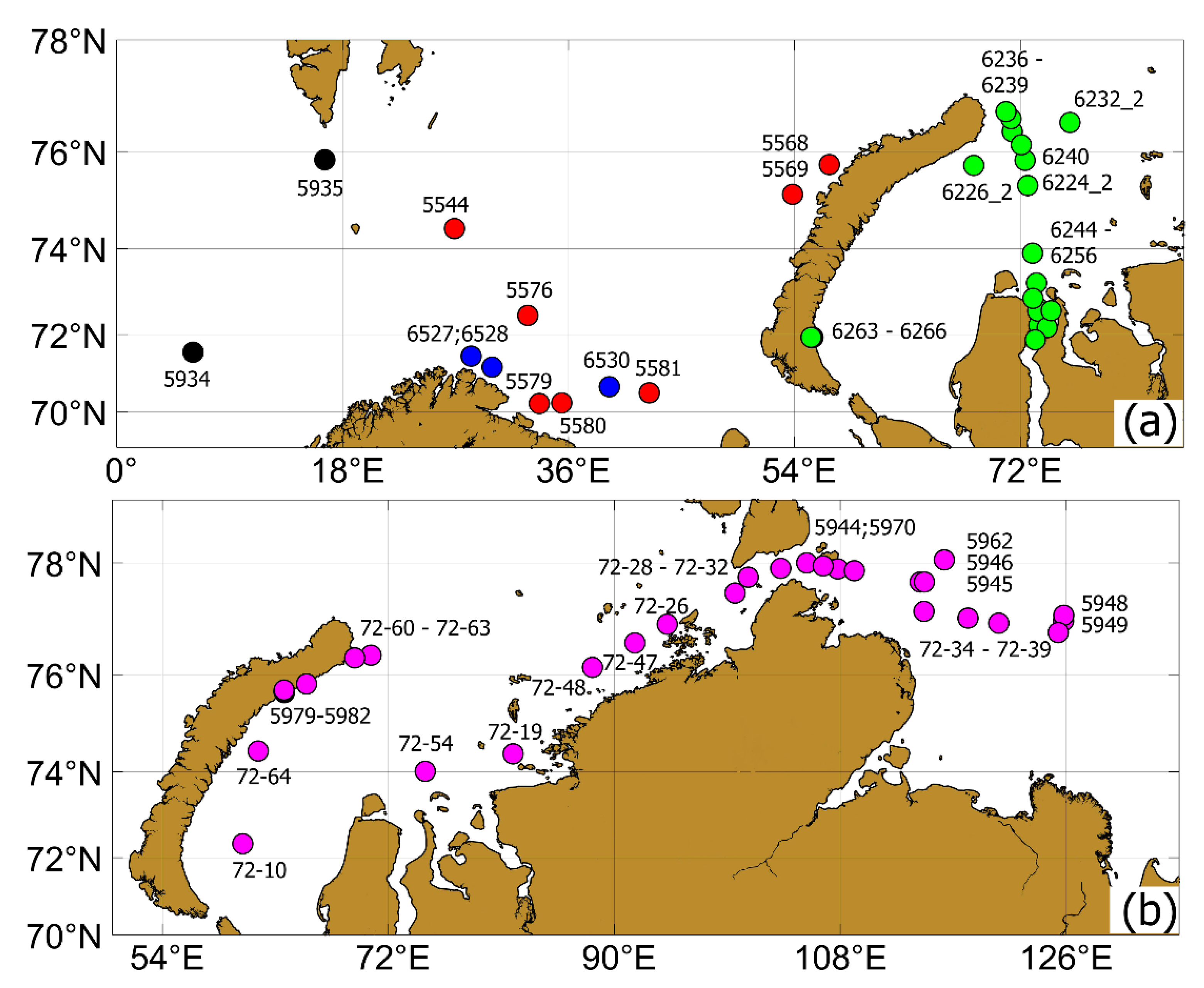
Figure 1.
Location of the selected stations: (a)—AMK-65 (blue), AMK-68 (red), AMK-71 (black), AMK-76 (green), (b)—AMK-72 (magenta).
Figure 1.
Location of the selected stations: (a)—AMK-65 (blue), AMK-68 (red), AMK-71 (black), AMK-76 (green), (b)—AMK-72 (magenta).
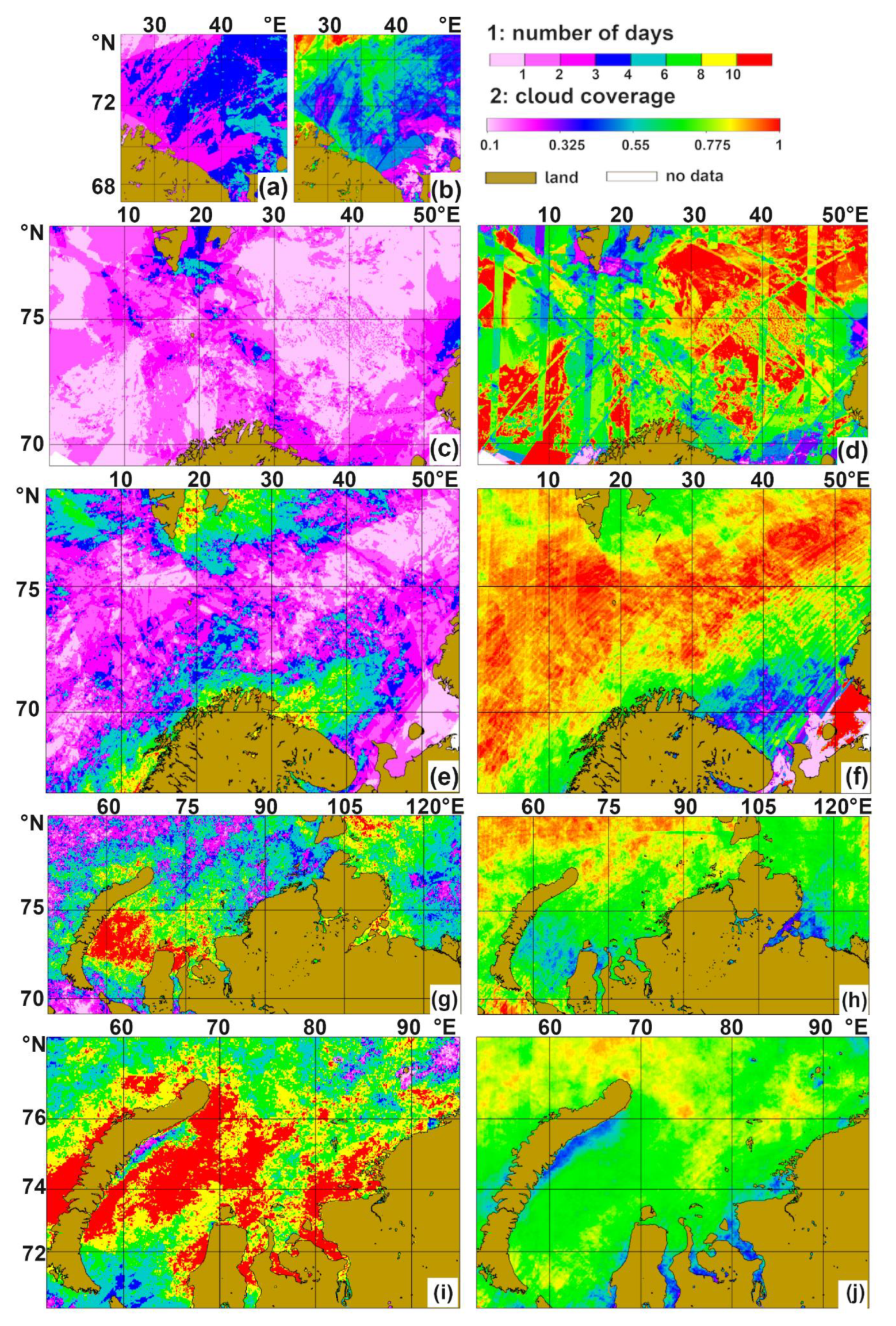
Figure 2.
Distributions of the number of days with data per bin (a,c,e; scale 1) and cloud coverage according to OLCI_CLOUD flag data (b,d,f; scale 2). AMK-65: (a,b); AMK-68: (c,d); AMK-71: (e,f), AMK-72: (g,h), AMK-76: (i,j).
Figure 2.
Distributions of the number of days with data per bin (a,c,e; scale 1) and cloud coverage according to OLCI_CLOUD flag data (b,d,f; scale 2). AMK-65: (a,b); AMK-68: (c,d); AMK-71: (e,f), AMK-72: (g,h), AMK-76: (i,j).
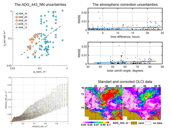
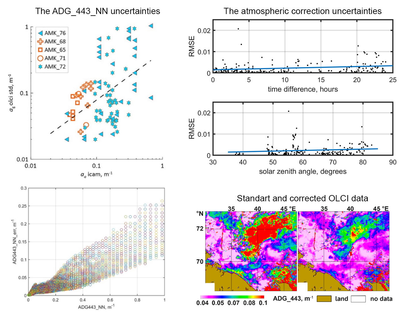
Figure 3.
Top: scatter plots of the in situ measured and satellite derived ag(443) values: (a)—complete dataset; (b)—river estuary data excluded. The Barents Sea points are shown in orange, the Kara and Laptev seas are shown in turquoise. Various cruises are represented by symbols. The dotted line is the correlation across all data. Bottom: the standard product errors ADG_443_NN_err in comparison with the ADG_443_NN values for OLCI Level 2 file S3A_OL_2_WFR_20170814T091713; (c) complete dataset; (d) the same in the enlarged scale. The Barents Sea, 14 August 2017.
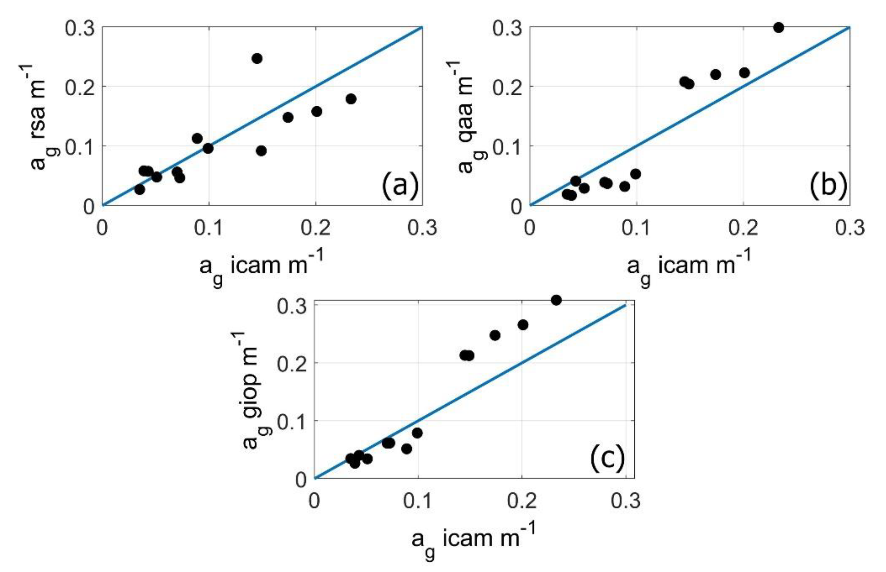
Figure 4.
Comparison of the absorption values calculated from the
Rrs measurements by the floating (or deck) spectroradiometer using different algorithms with the values measured by the ICAM device for 13 stations. The solid line is 1:1 dependency. (
a)—RSA algorithm (RMSE = 0.042, RE = 40%); (
b) QAA (RMSE = 0.04, RE = 38%); (
c)—GIOP (RMSE = 0.045, RE = 36%) (see
Section 2.3).
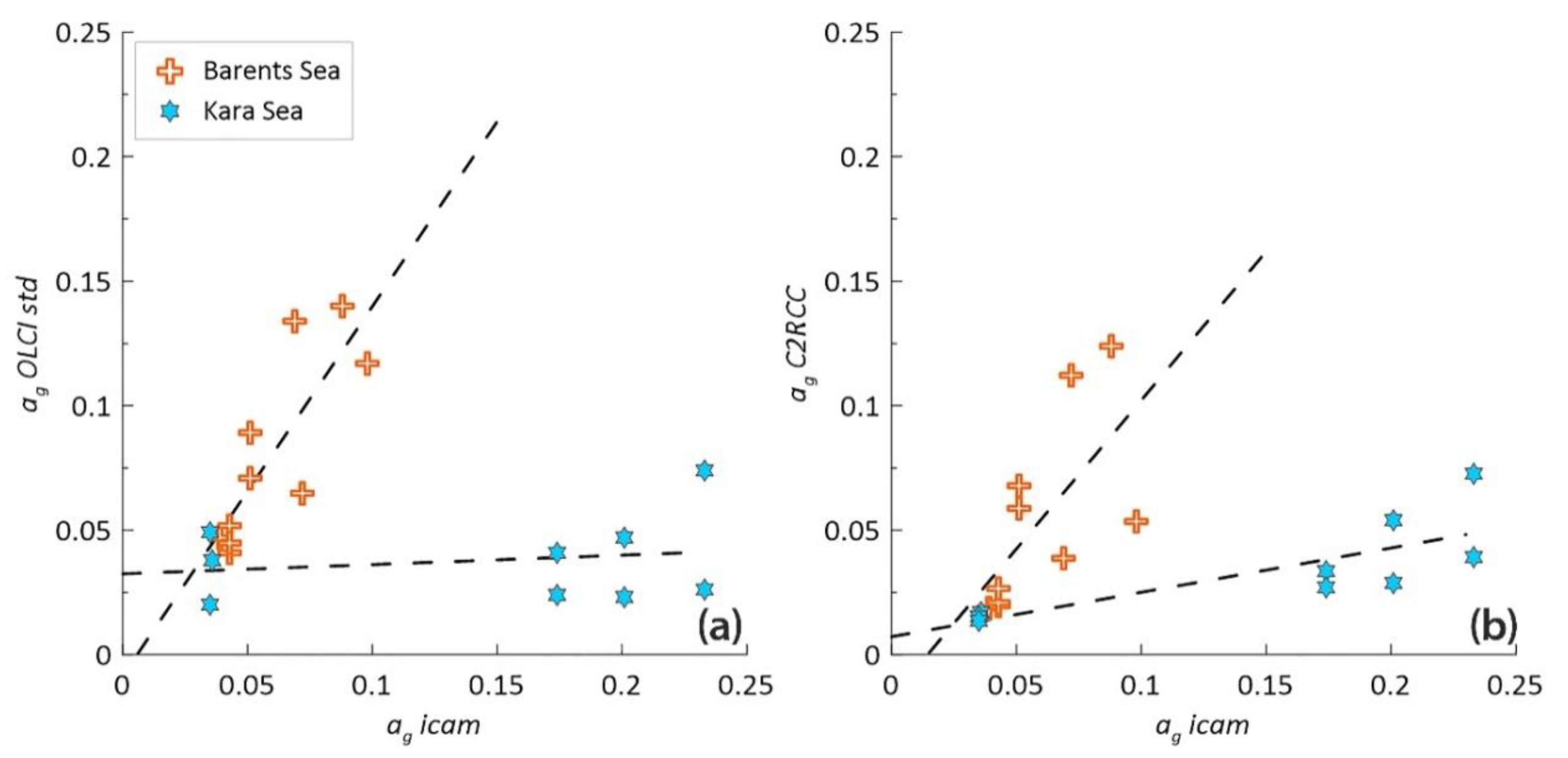
Figure 5.
Regressions of satellite values ag_olci_std (a) and ag_olci_C2RCC (b) vs. measured values ag_icam. The dotted lines represent the correlations for the corresponding seas.
Figure 5.
Regressions of satellite values ag_olci_std (a) and ag_olci_C2RCC (b) vs. measured values ag_icam. The dotted lines represent the correlations for the corresponding seas.
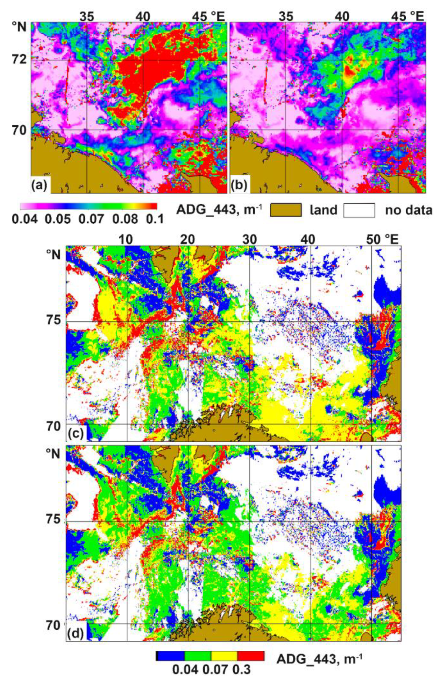
Figure 6.
The ADG_443_NN distributions based on standard OLCI data ag_olci_std (a,c) and corrected ag_corr data (b,d) for the AMK-65 (a,b) and AMK-68 (c,d) cruises.
Figure 6.
The ADG_443_NN distributions based on standard OLCI data ag_olci_std (a,c) and corrected ag_corr data (b,d) for the AMK-65 (a,b) and AMK-68 (c,d) cruises.
Figure 7.
Dependences of the average RMSE of the Rrs values on the absolute difference between the time of the in situ and the satellite measurements (A) and on the zenith angle of the sun (B). The blue lines show the trend assessment.
Figure 7.
Dependences of the average RMSE of the Rrs values on the absolute difference between the time of the in situ and the satellite measurements (A) and on the zenith angle of the sun (B). The blue lines show the trend assessment.
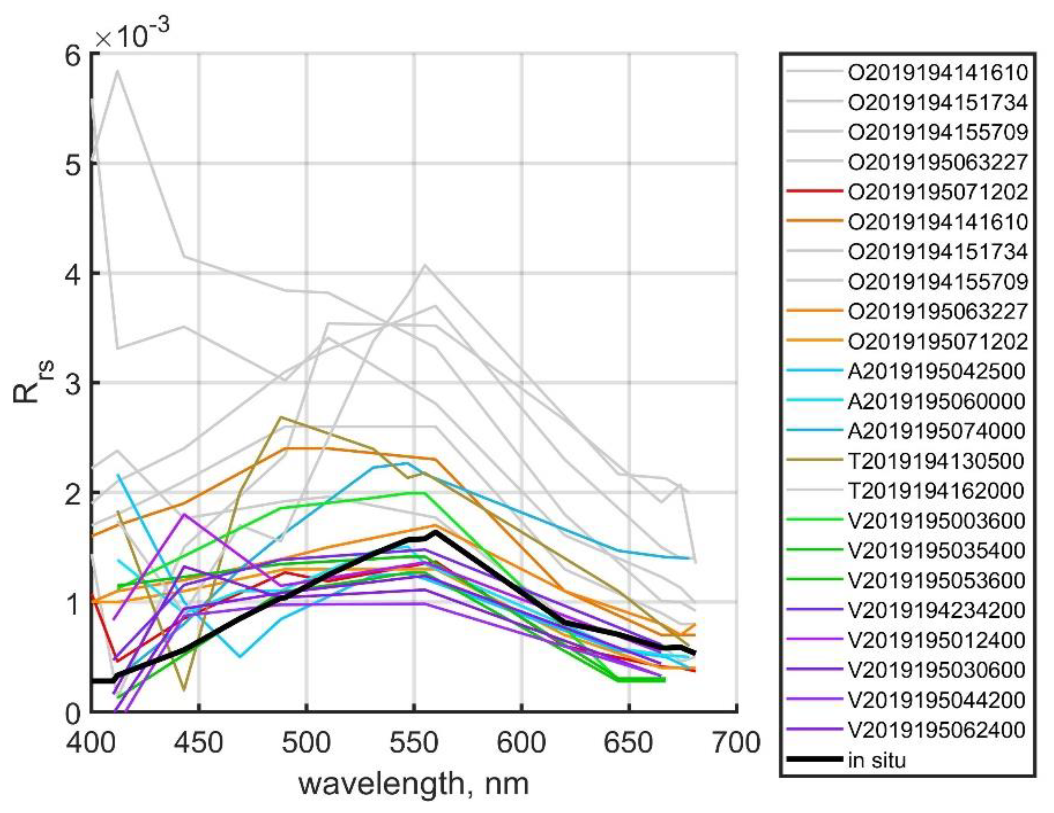
Figure 8.
Rrs(λ) values obtained from the shipboard (black line) and satellite measurements (colored lines: red—OLCI BAC, orange—OLCI AAC, blue—MODIS Aqua, brown—MODIS Terra, green—VIIRS SNPP, purple—VIIRS NOAA-20). The grey color shows data for which the RMSE values obtained by comparing shipboard and satellite data were greater than 0.001. Station 6240, Kara Sea, 14 July 2019.
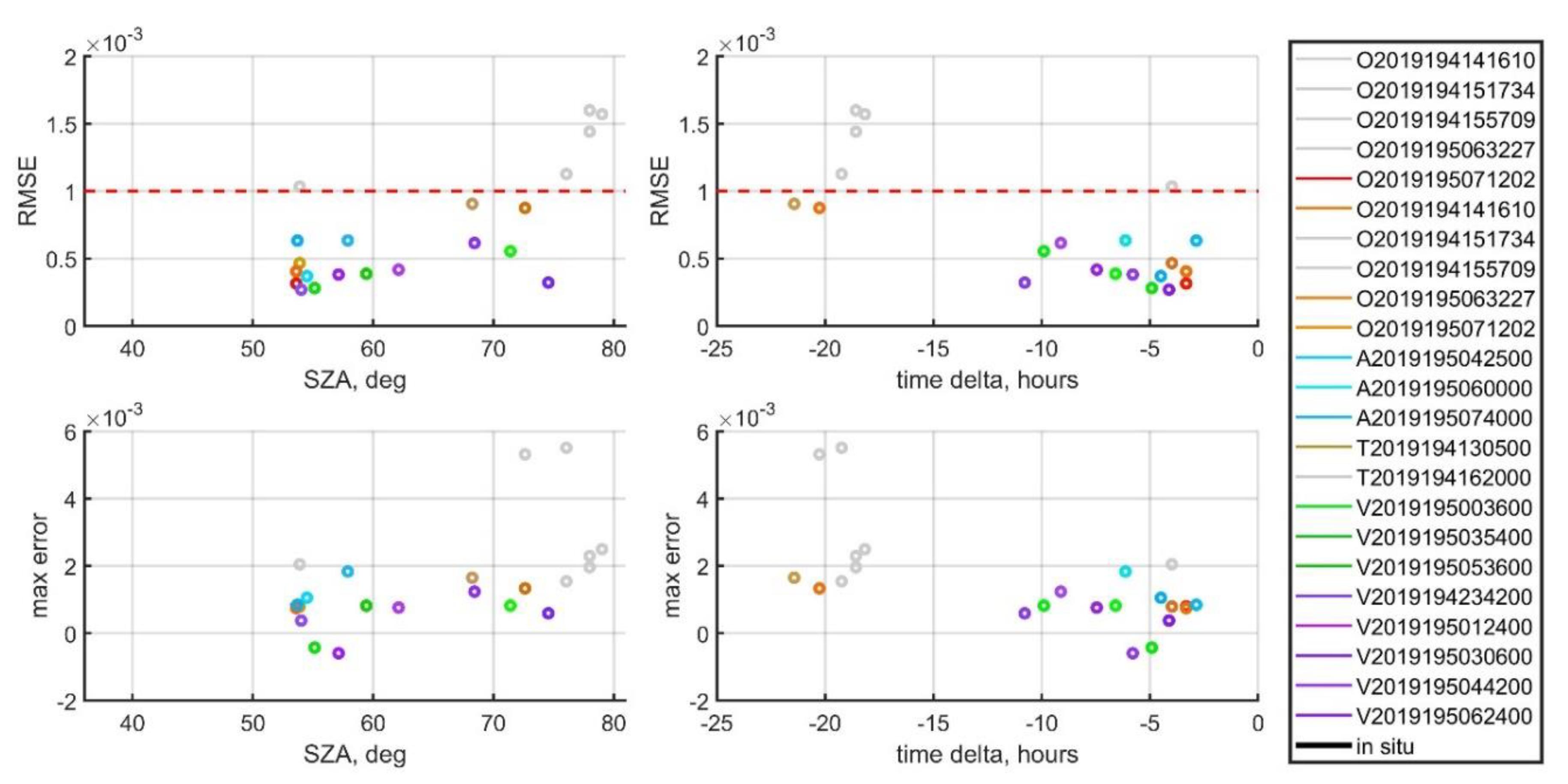
Figure 9.
RMSE (top row) and maximum error (bottom row) values obtained when comparing shipboard and satellite data depending on the sun zenith angle (left column) and the time interval between data (right column). The colors of the circles correspond to the colors of the lines in
Figure 1. The gray circles show the data for which the RMSE values exceed 0.001. The red dotted line on the right side of the figure corresponds to RMSE = 0.001. Station 6240, Kara Sea, 14 July 2019.
Figure 10.
Spatial distribution of the beam attenuation coefficient c measured in the Kara Sea on 14 July 2019. The dotted line shows the position of station 6240.
Figure 10.
Spatial distribution of the beam attenuation coefficient c measured in the Kara Sea on 14 July 2019. The dotted line shows the position of station 6240.
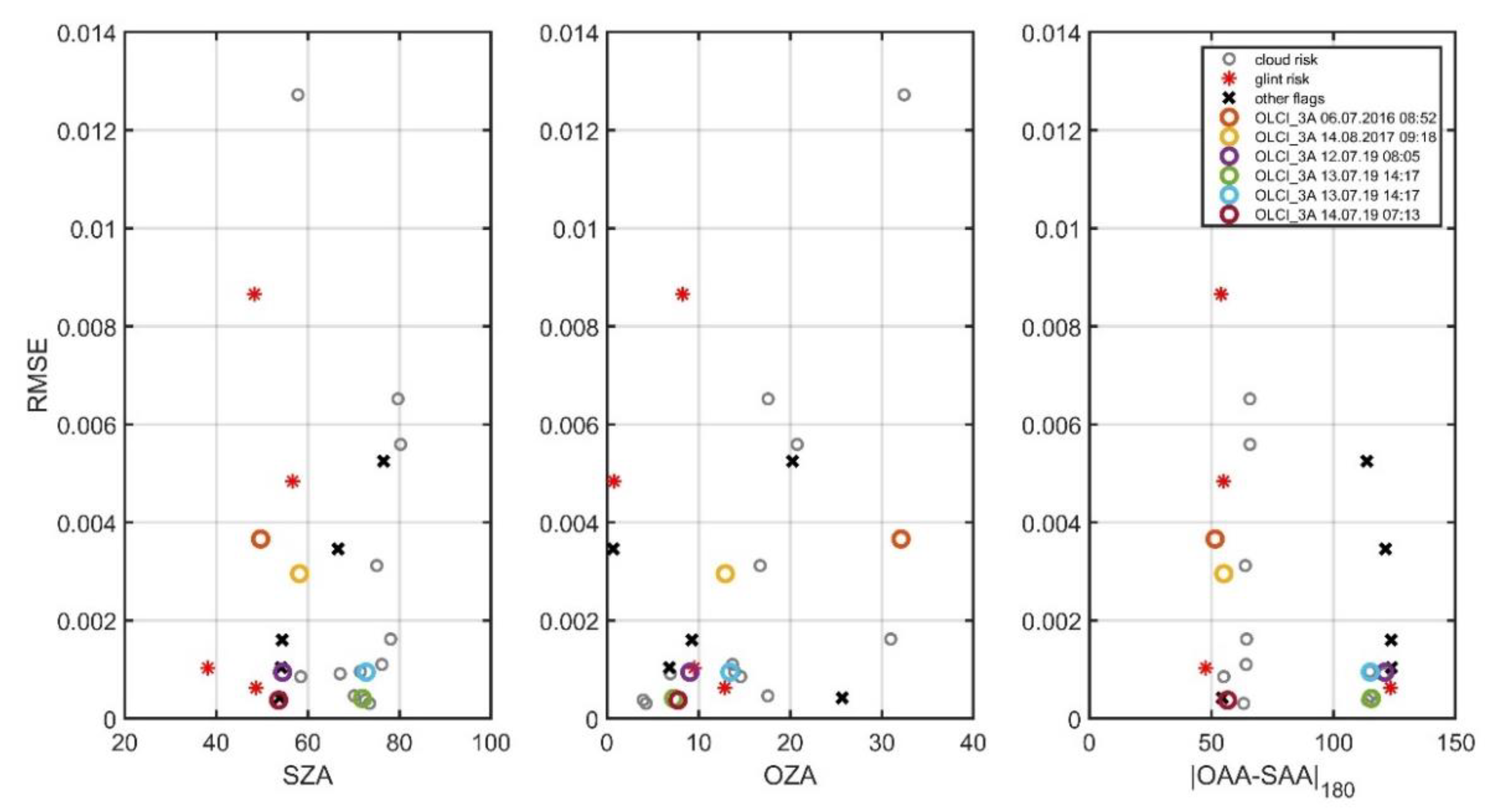
Figure 11.
Average RMSE values obtained by comparing shipboard and satellite data for 15 ship stations and 27 OLCI spectra calculated using the C2RCC processor, depending on the solar zenith angle (left), observation zenith angle (center), and the absolute values of azimuth angle differences (right). Gray circles indicate the cloud risk flag, red asterisks—glint risk, black crosses—any other flag, colored circles—data without flags.
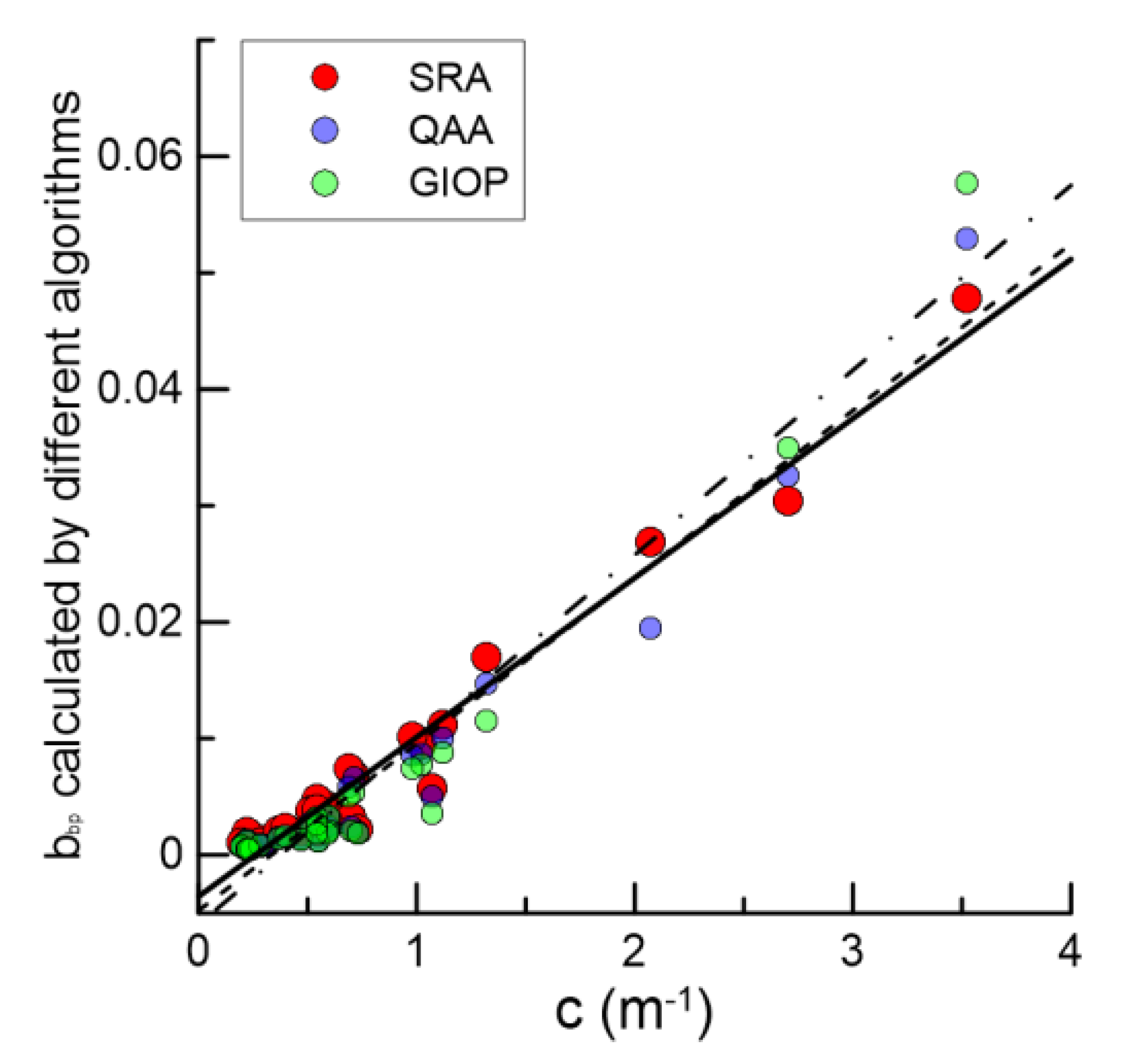
Figure 12.
Comparison of the particle backscattering coefficient bbp(555) with the beam attenuation coefficient c(530) for the Barents Sea. Red circles—SRA algorithm, blue—QAA algorithm, green—GIOP algorithm. The black line is a correlation based on SRA, black dotted line—correlation based on QAA data, dash-dotted line – based on GIOP data.
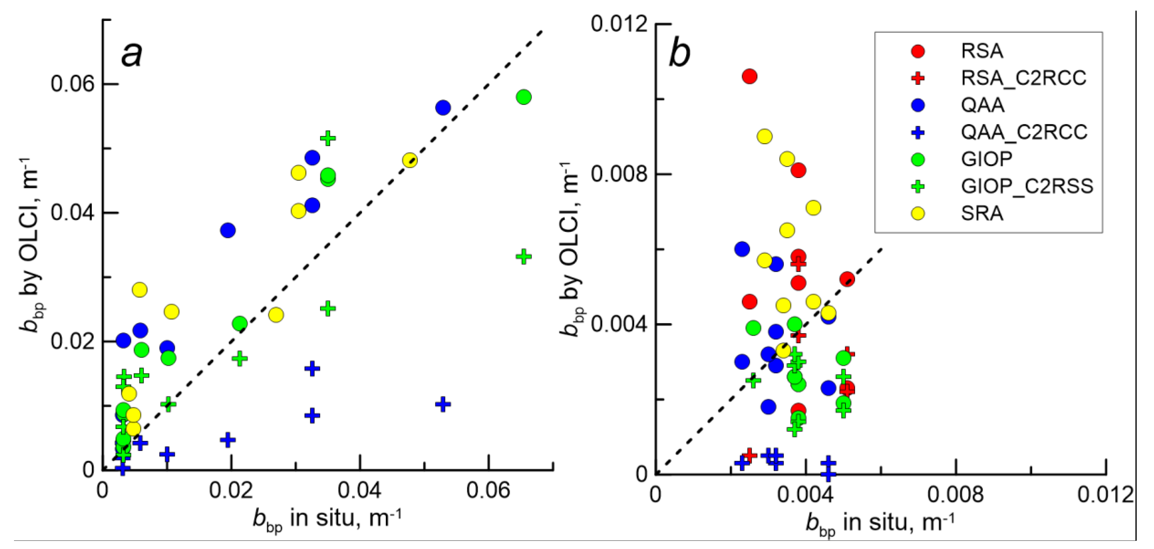
Figure 13.
Scatterplots of in situ bbp(555) data and data from satellite calculations for the Barents Sea (a), the Kara Sea, and the Laptev Sea (b). Red circles—RSA algorithm for the Level 2 data, red crosses—RSA_C2RCC algorithm; blue circles—QAA algorithm for the Level 2 data, blue crosses—QAA_C2RCC algorithm; green circles—GIOP algorithm for the Level 2 data, green crosses—GIOP _C2RCC algorithm; yellow circles—SRA. Dashed lines—1: 1 match.
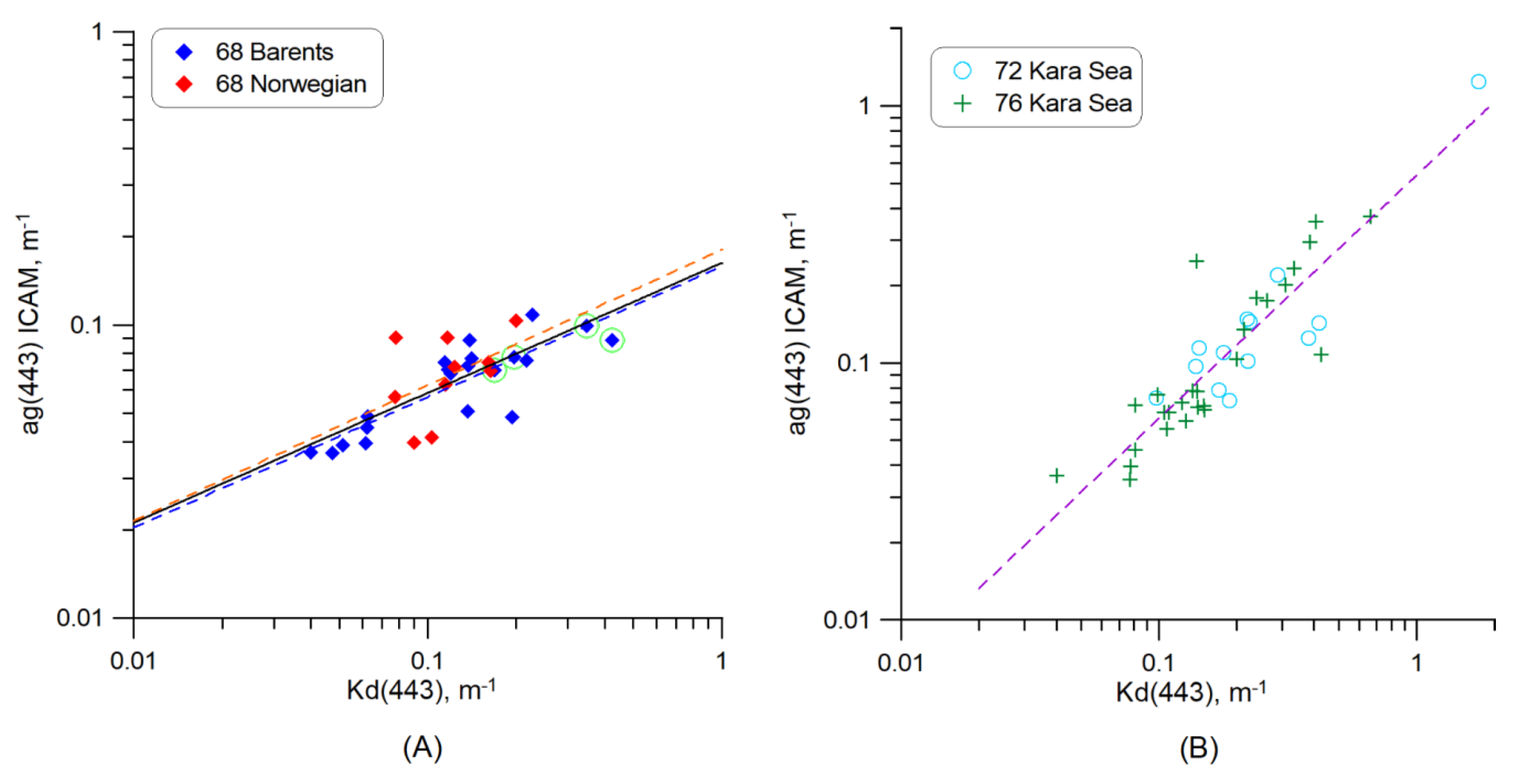
Figure 14.
Comparison of the yellow substance absorption coefficient ag(443) and the diffuse attenuation coefficient Kd(443) measured in situ: (A) for the Barents and Norwegian seas (AMK 68); (B) the Kara Sea (AMK 72 and 76). The solid black line is the regression line for all AMK 68 data; blue dotted line—the Barents Sea, AMK 68; red dotted line—the Norwegian Sea, AMK 68; purple dotted line—the Kara Sea, AMK 72 and 76. Green circles show the stations with coccolithophore blooms.
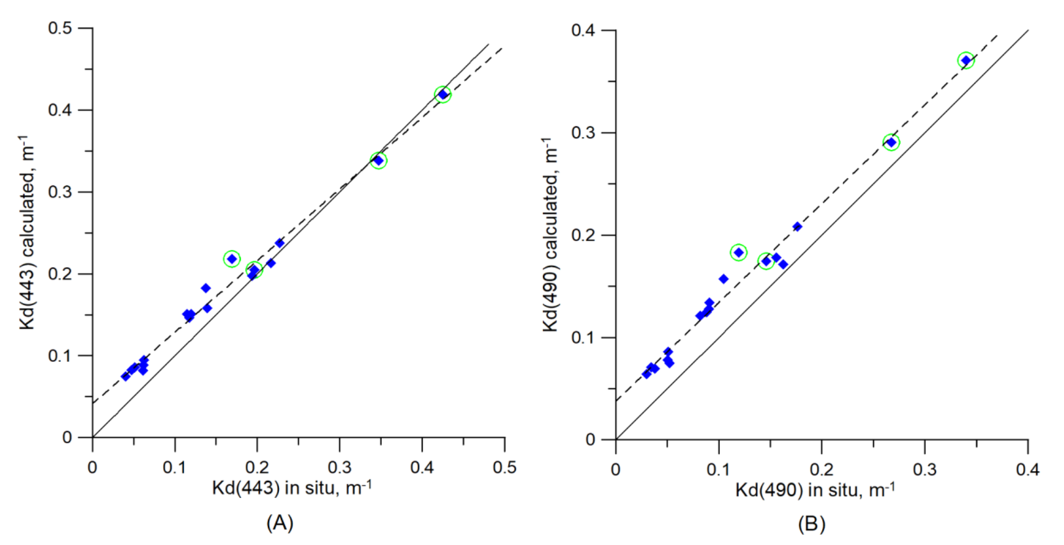
Figure 15.
Scatterplot of the diffuse attenuation coefficient
Kd for the wavelengths 443 (
A) and 490 (
B) nm calculated by formula [
52], and from in situ measurements of underwater irradiance at 18 stations in the Barents Sea (AMK 68). Solid black line—perfect correspondence 1:1; dotted black line—linear regression. Green circles show the stations with coccolithophore blooms.
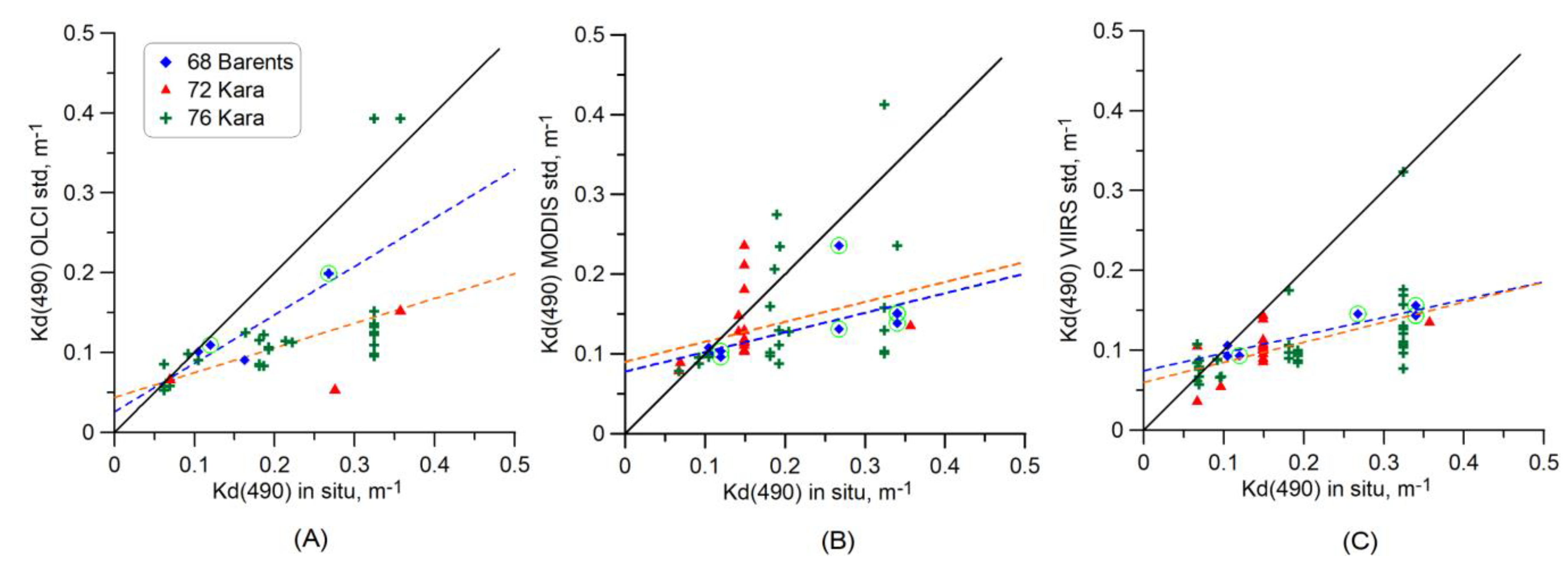
Figure 16.
Scatterplot of the diffuse attenuation coefficient Kd(490) values calculated from field measurements and satellite data (standard algorithm, nearest pixel): (A) OLCI; (B) MODIS; (C) VIIRS. Solid black line—perfect correspondence 1:1; dotted blue line—the regression line for the Barents Sea, AMK 68; dotted red line—the Kara Sea, AMK 72, and 76. Green circles show the stations with coccolithophore blooms.
Table 1.
The Arctic and Atlantic R/V AMK voyages with measured data.
Table 1.
The Arctic and Atlantic R/V AMK voyages with measured data.
| Cruise and Vessel | Region | Measurement Period | Number of Stations |
|---|
| AMK-65 | Norwegian and Barents Seas | 29 June–9 July 2016 | 14 |
| AMK-68 | North Atlantic (60°N section), Barents Sea | 30 June–7 August 2017 | 72 |
| AMK-71 | North Atlantic (60°N section), Norwegian and Barents seas | 28 June–13 August 2018 | 75 |
| AMK-72 | Kara Sea and Laptev Sea | 20 August–16 September 2018 | 105 |
| AMK-76 | Kara Sea | 7–28 July 2019 | 47 |
Table 2.
Regression parameters between the absorption values derived from satellite and in situ data for various algorithms and neural networks (NN) OLCI. N is the number of pairs to calculate the regression, R2 is the coefficient of determination.
Table 2.
Regression parameters between the absorption values derived from satellite and in situ data for various algorithms and neural networks (NN) OLCI. N is the number of pairs to calculate the regression, R2 is the coefficient of determination.
| | MODIS | VIIRS | OLCI |
|---|
| | Aqua | Terra | SNPP | NOAA-20 | Standard | C2RCC |
|---|
| | N * | R2 | N | R2 | N | R2 | N | R2 | N | R2 | N | R2 |
| RSA | 21 | 0.52 | 23 | 0.44 | 23 | 0.38 | 12 | 0.29 | 18 | 0.04 | 14 | 0.24 |
| QAA | 21 | 0.27 | 15 | 0.03 | 20 | 0.55 | 8 | 0.13 | 18 | 0 | 19 | 0.47 |
| GIOP | 24 | 0.02 | 30 | 0.2 | 30 | 0.08 | 13 | 0.02 | 19 | 0.08 | 19 | 0.33 |
| NN | | | | | | | | | 19 | 0.04 | 19 | 0.03 |
Table 3.
Regression parameters of the absorbance values calculated from OLCI data (
ag_olci_std, m
−1 (
Figure 5a) and
ag_olci_C2RCC (
Figure 5b)) versus those measured by ICAM (
ag_icam), m
−1.
Table 3.
Regression parameters of the absorbance values calculated from OLCI data (
ag_olci_std, m
−1 (
Figure 5a) and
ag_olci_C2RCC (
Figure 5b)) versus those measured by ICAM (
ag_icam), m
−1.
| Sea | N | Regression Equation | <X> | <Y> | R2 | Sregr | RE *, % |
|---|
| OLCI_standard vs. ag_ICAM |
| Barents | 10 | Y = 1.48 X − 0.008 | 0.06 | 0.08 | 0.670 | 0.023 | 28 |
| Kara | 9 | Y = 0.037 X + 0.032 | 0.147 | 0.038 | 0.035 | insignificant | - |
| OLCI_C2RCC vs. ag_ICAM |
| Barents | 10 | Y = 1.19 X − 0.017 | 0.06 | 0.054 | 0.430 | 0.03 | 56 |
| Kara | 9 | Y = 0.178 X + 0.007 | 0.147 | 0.033 | 0.624 | 0.012 | 38 |
Table 4.
Regression equations for calculation of the absorption coefficient from OLCI data.
Table 4.
Regression equations for calculation of the absorption coefficient from OLCI data.
| Sea | N | Regression Equation | <X> | <Y> | R2 | s_regr. | RE, % |
|---|
| ag_corr vs. OLCI_standard | |
| Barents | 10 | Y = 0.67 X + 0.020 | 0.06 | 0.06 | 0.670 | 0.010 | 17 |
| ag_corr vs. OLCI_C2RCC | |
| Barents | 10 | Y = 0.43 X + 0.034 | 0.06 | 0.06 | 0.430 | 0.011 | 18 |
| Kara | 9 | Y = 0.62 X + 0.055 | 0.147 | 0.147 | 0.624 | 0.045 | 30 |
Table 5.
The total number of satellite data points for 15 stations with shipboard reflectance measurements and their number with RMSE ≤ 0.001. AAC—Alternative Atmospheric Correction, BAC—Baseline Atmospheric Correction.
Table 5.
The total number of satellite data points for 15 stations with shipboard reflectance measurements and their number with RMSE ≤ 0.001. AAC—Alternative Atmospheric Correction, BAC—Baseline Atmospheric Correction.
| Sensor | All Data | RMSE ≤ 0.001 |
|---|
| OLCI BAC | 27 | 3 |
| OLCI AAC | 27 | 13 |
| MODIS Aqua | 36 | 16 |
| MODIS Terra | 40 | 13 |
| VIIRS SNPP | 37 | 14 |
| VIIRS NOAA-20 | 22 | 18 |
Table 6.
The statistical parameters of the regression bbp(555) (Y) vs. c(530) (X) with different algorithms.
Table 6.
The statistical parameters of the regression bbp(555) (Y) vs. c(530) (X) with different algorithms.
| Algorithm | N | Regression | <X> | <Y> | R2 | RMSE, m−1 | RE, % |
|---|
| SRA | 31 | Y = 0.01 X − 0.004 | 0.78 | 0.01 | 0.96 | 0.0020 | 29 |
| QAA | 31 | Y = 0.014 X − 0.005 | 0.78 | 0.01 | 0.95 | 0.0026 | 40 |
| GIOP | 29 | Y = 0.02 X − 0.006 | 0.75 | 0.005 | 0.94 | 0.0031 | 51 |
Table 7.
Regression parameters between bbp(555) from satellite (Y) and in situ (X) data for different algorithms (only cases where the values of the coefficient of determination exceed 0.3).
Table 7.
Regression parameters between bbp(555) from satellite (Y) and in situ (X) data for different algorithms (only cases where the values of the coefficient of determination exceed 0.3).
| Algorithm X | Algorithm Y | Seas | N | Regression | <X> | <Y> | R2 | RMSE, m−1 | RE, % |
|---|
| QAA | Standard | Barents | 11 | Y = 1.01 X + 0.01 | 0.02 | 0.03 | 0.87 | 0.0072 | 28 |
| QAA | C2RCC | Barents | 11 | Y = 0.21 X + 0.002 | 0.02 | 0.005 | 0.61 | 0.0031 | 54 |
| QAA | C2RCC | Kara and Laptev | 9 | Y = −0.11 X + 0.001 | 0.003 | 0.0003 | 0.33 | 0.0002 | 56 |
| GIOP | Standard | Barents | 11 | Y = 0.89 X + 0.01 | 0.02 | 0.02 | 0.92 | 0.0059 | 26 |
| GIOP | C2RCC | Barents | 11 | Y = 0.52 X + 0.01 | 0.02 | 0.02 | 0.56 | 0.0102 | 54 |
| SRA | SRA | Barents | 11 | Y = 0.86 X + 0.01 | 0.02 | 0.03 | 0.75 | 0.0084 | 32 |
Table 8.
Regression parameters between values of ag and Kd measured in situ at a wavelength of 443 nm.
Table 8.
Regression parameters between values of ag and Kd measured in situ at a wavelength of 443 nm.
| Data Set | N | Regression Equation | R2 |
|---|
| Barents Sea, AMK 68 | 20 | ag = 0.16 Kd 0.44 | 0.72 |
| Norwegian Sea, AMK 68 | 10 | ag = 0.18 Kd 0.46 | 0.21 |
| all AMK 68 data | 30 | ag = 0.16 Kd 0.44 | 0.56 |
| Kara Sea, AMK 72 and 76 | 31 | ag = 0.55 Kd 0.94 | 0.73 |
Table 9.
Correspondence parameters between the Kd(490) values obtained from field measurements (X) and satellite data (Y). Satellite data for the nearest pixel.
Table 9.
Correspondence parameters between the Kd(490) values obtained from field measurements (X) and satellite data (Y). Satellite data for the nearest pixel.
| Data Set | Regression Equation | N * | R2 | <Y>/<X> | RMSE | RE |
|---|
| OLCI |
| AMK 68 | Y = 0.61 X + 0.03 | 4 | 0.80 | 0.76 | 0.05 | 20% |
| AMK 72 and 76 | Y = 0.31 X + 0.04 | 24 | 0.24 | 0.51 | 0.14 | 45% |
| MODIS |
| AMK 68 | Y = 0.25 X + 0.08 | 13 | 0.48 | 0.63 | 0.11 | 26% |
| AMK 72 and 76 | Y = 0.25 X + 0.09 | 32 | 0.09 | 0.74 | 0.09 | 33% |
| VIIRS |
| AMK 68 | Y = 0.22 X + 0.07 | 7 | 0.91 | 0.55 | 0.13 | 36% |
| AMK 72 and 76 | Y = 0.25 X + 0.06 | 49 | 0.31 | 0.58 | 0.14 | 47% |

 ,
, 


