Building Extraction from Airborne LiDAR Data Based on Min-Cut and Improved Post-Processing


Abstract
:1. Introduction
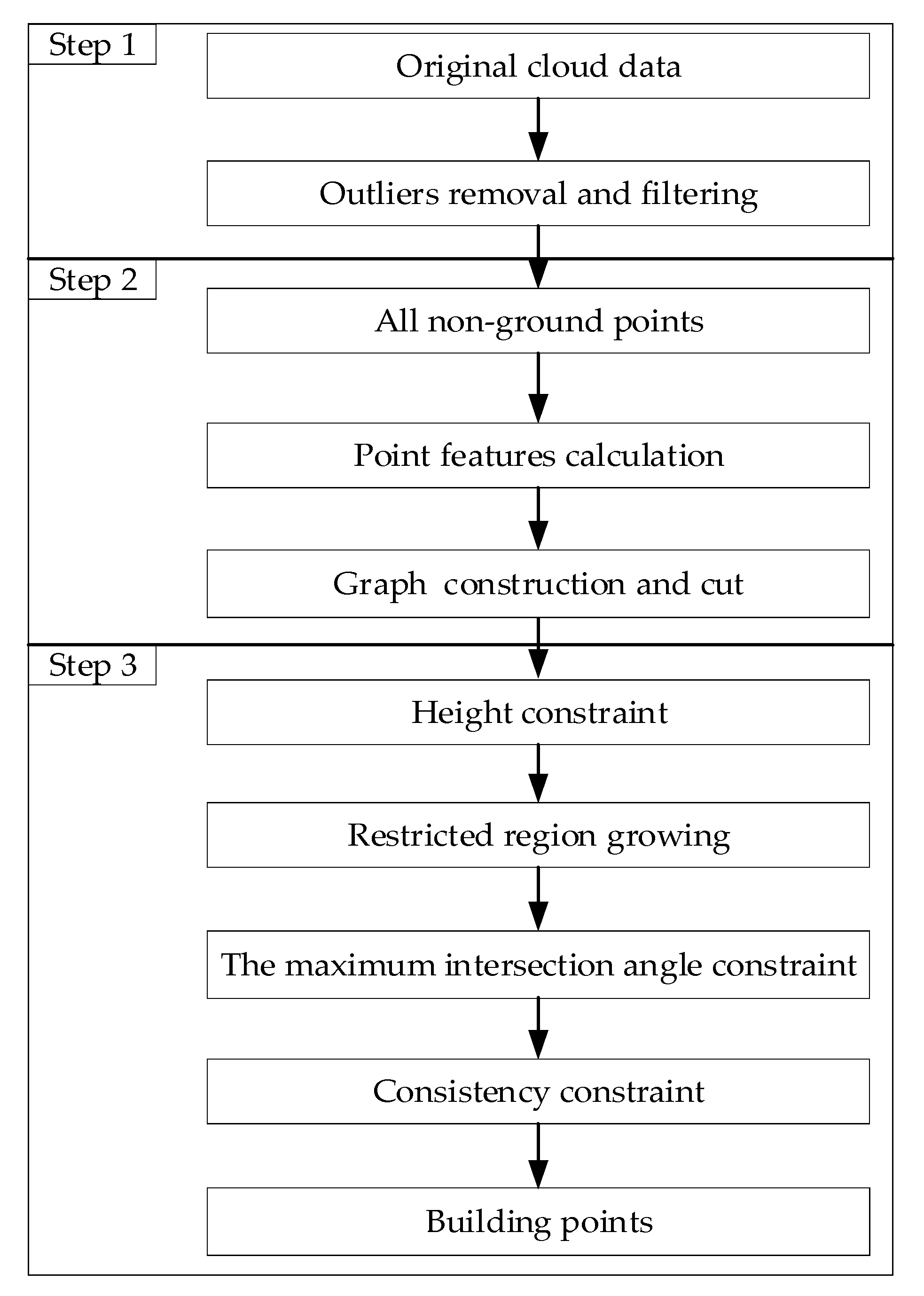
2. Methodology
2.1. Outliers Removal and Filtering
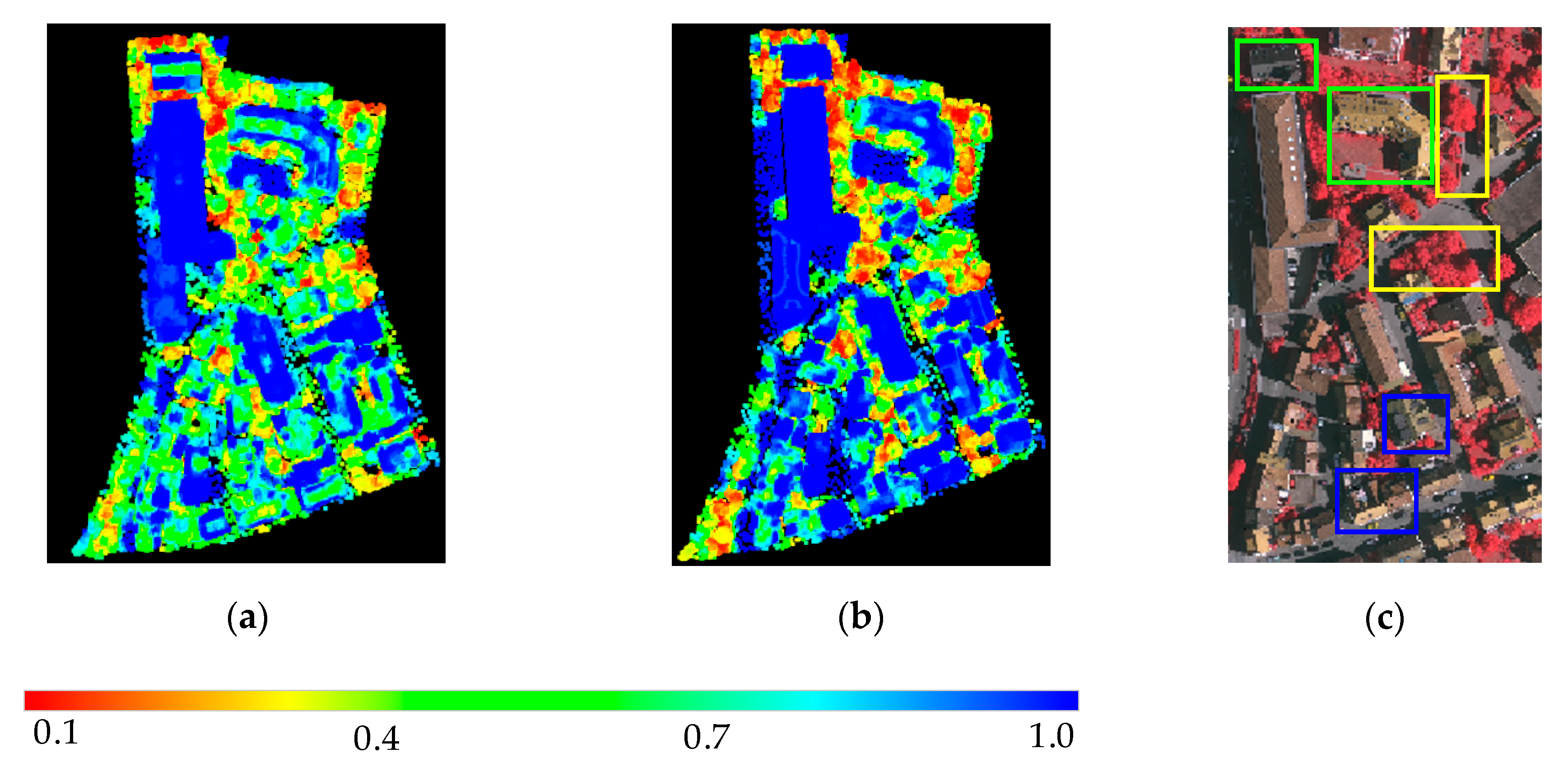
2.2. Point Features Calculation and Normalization
2.2.1. Curvature Feature
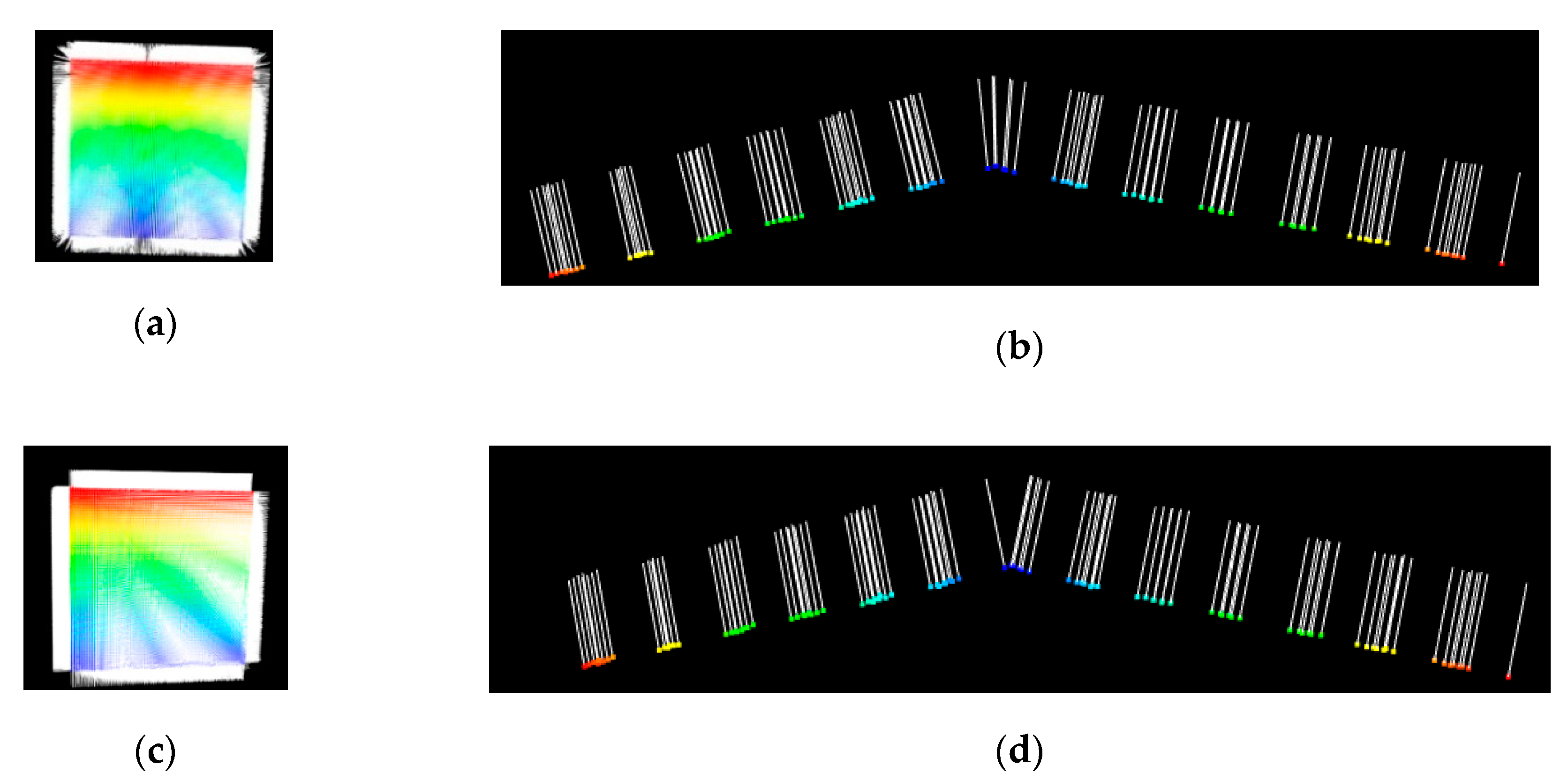
2.2.2. Variance of LRSC-Based Normal Vector Feature
2.2.3. Feature Normalization
2.2.4. Graph Construction and Cut
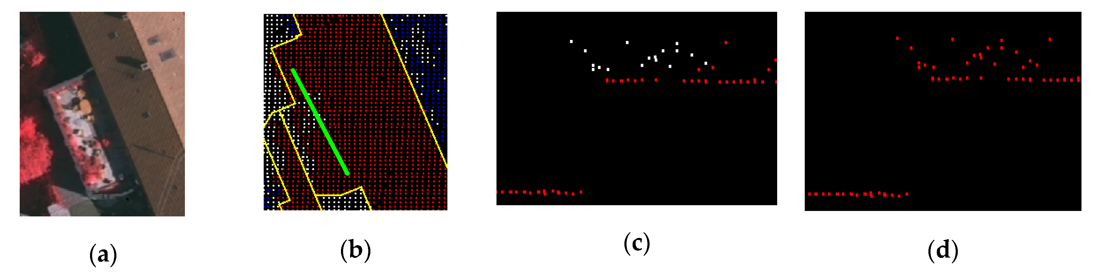
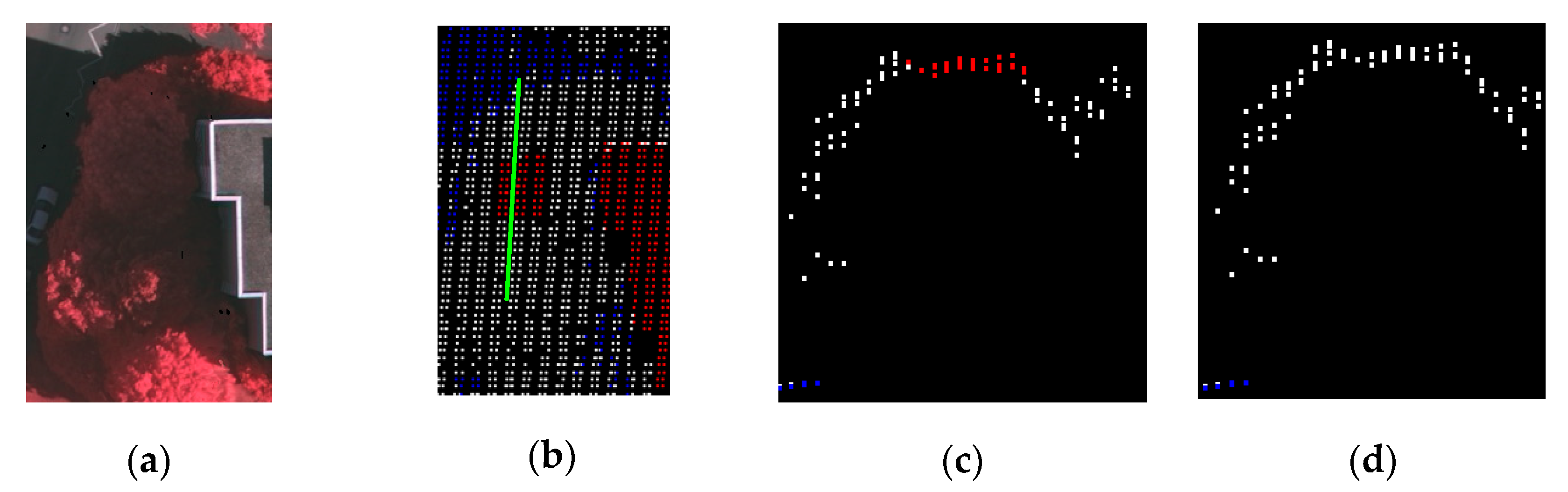
2.3. Improved Post-Processing
2.3.1. Height Constraint
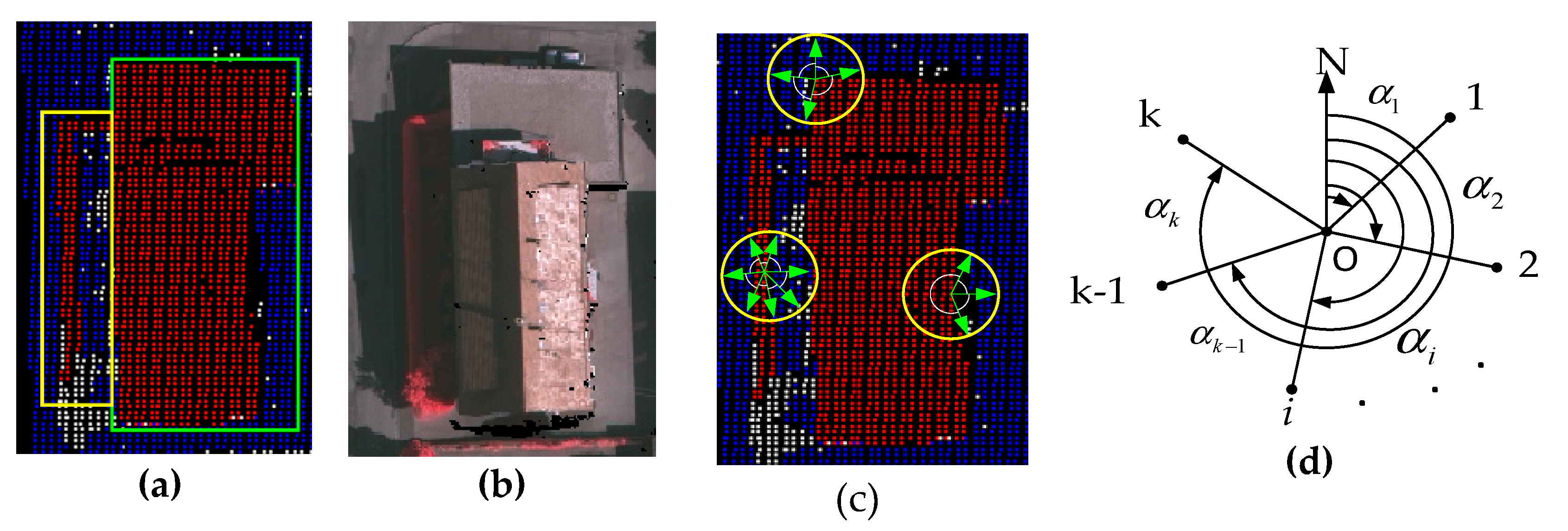
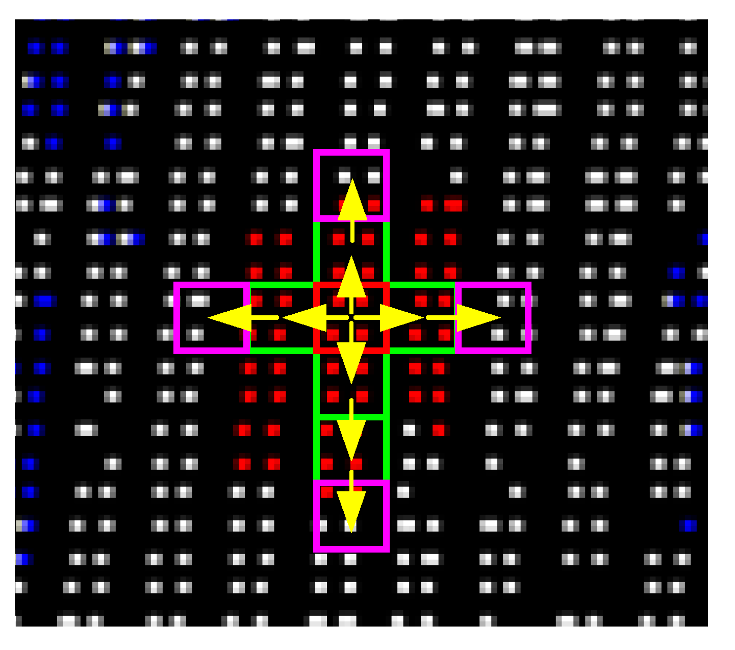
2.3.2. Restricted Region Growing
2.3.3. Maximum Intersection Angle Constraint
2.3.4. Consistency Constraint
3. Experimental Results and Analysis
3.1. Experiments on the ISPRS Benchmark Dataset
3.1.1. Data Description
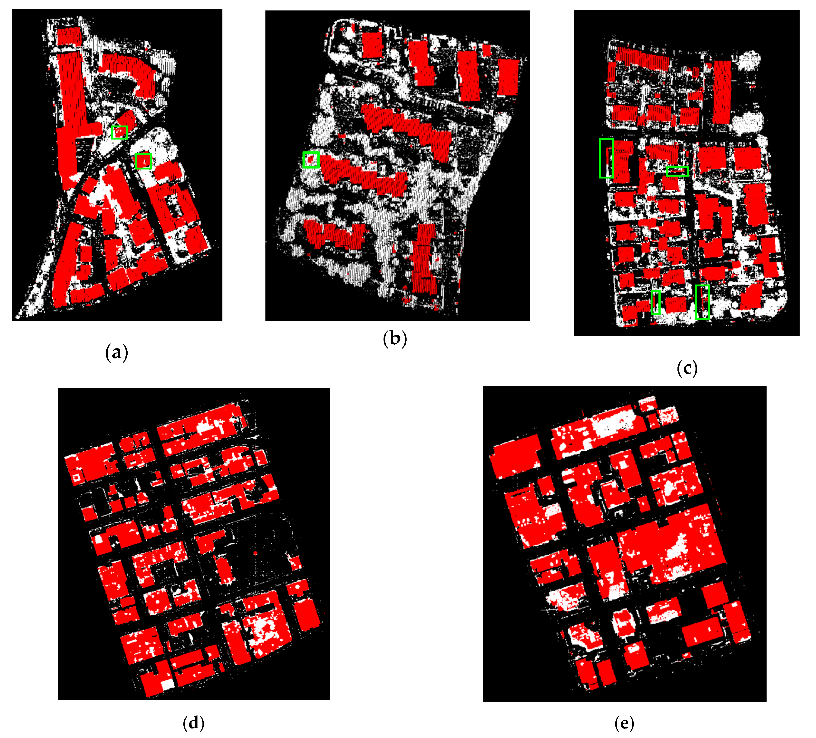
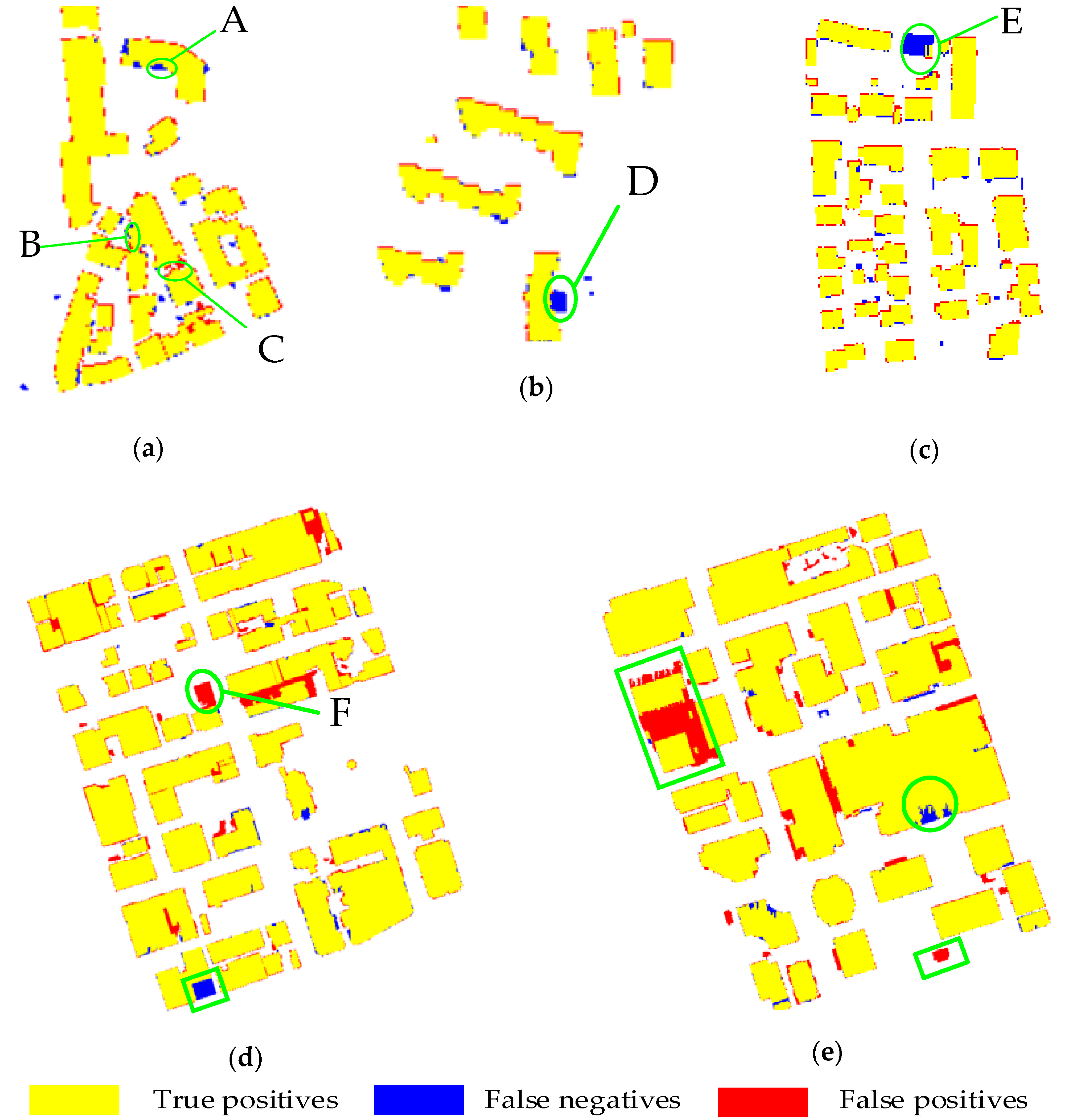
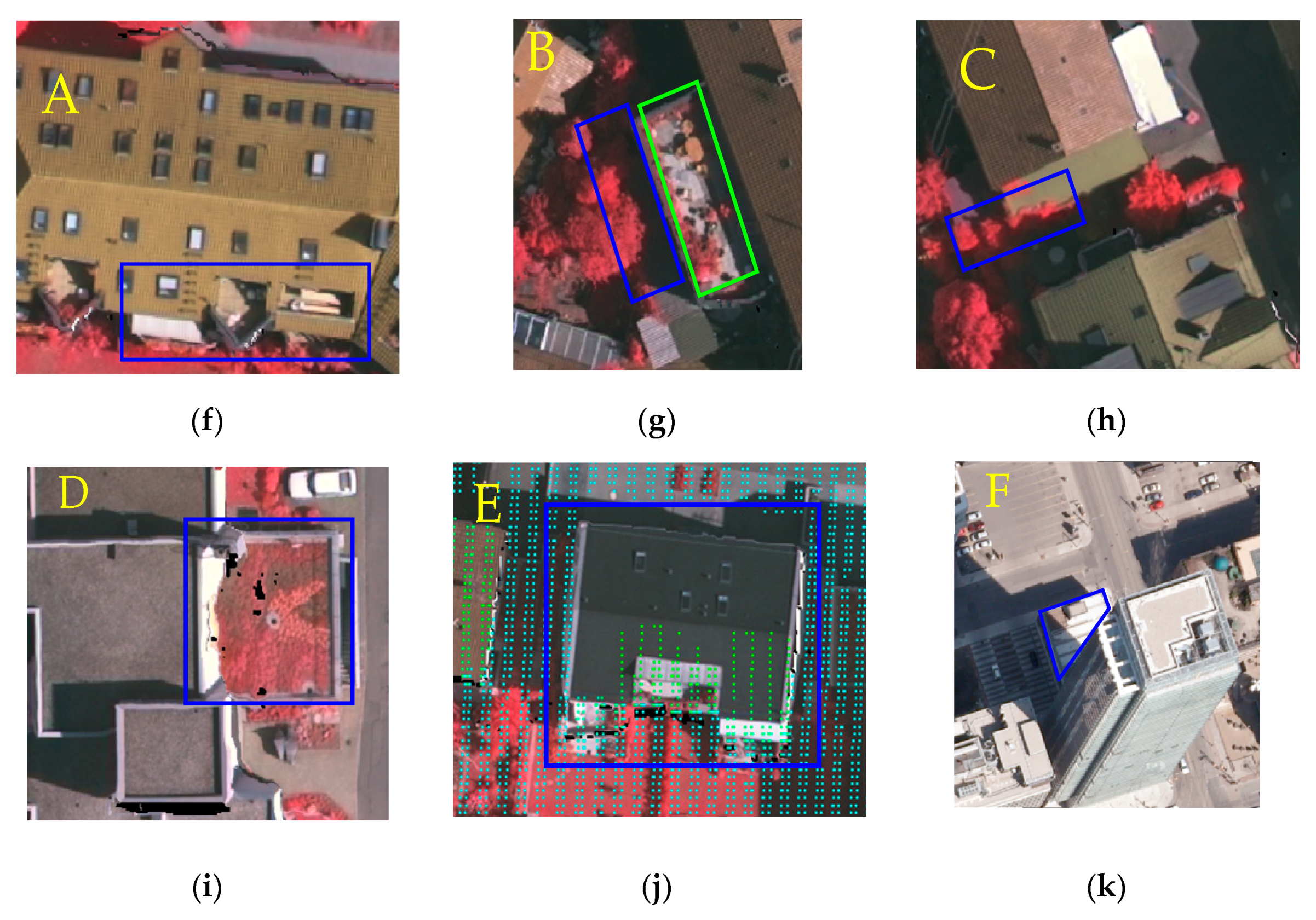
3.1.2. Results and Analysis
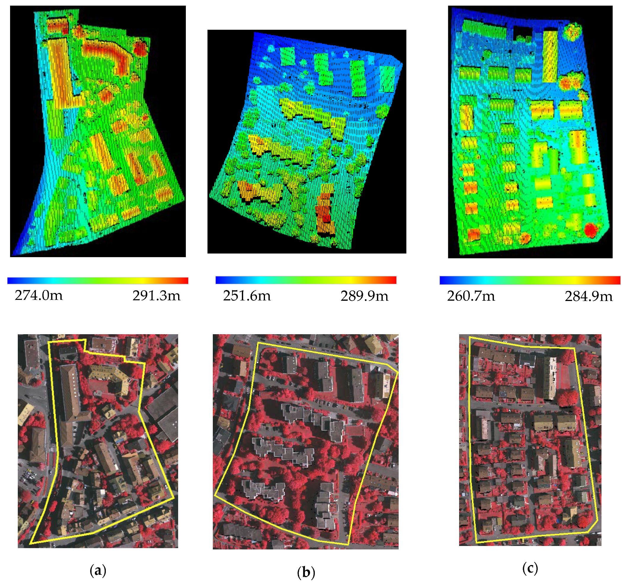
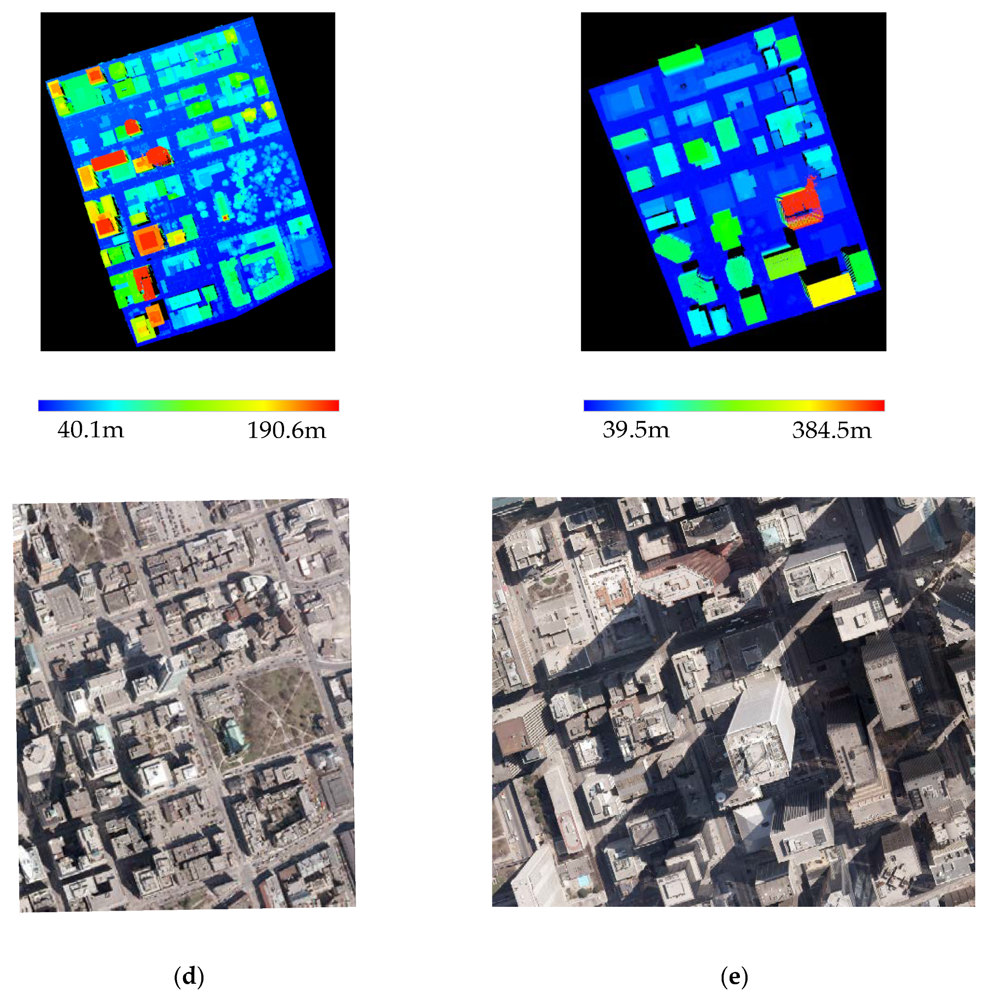
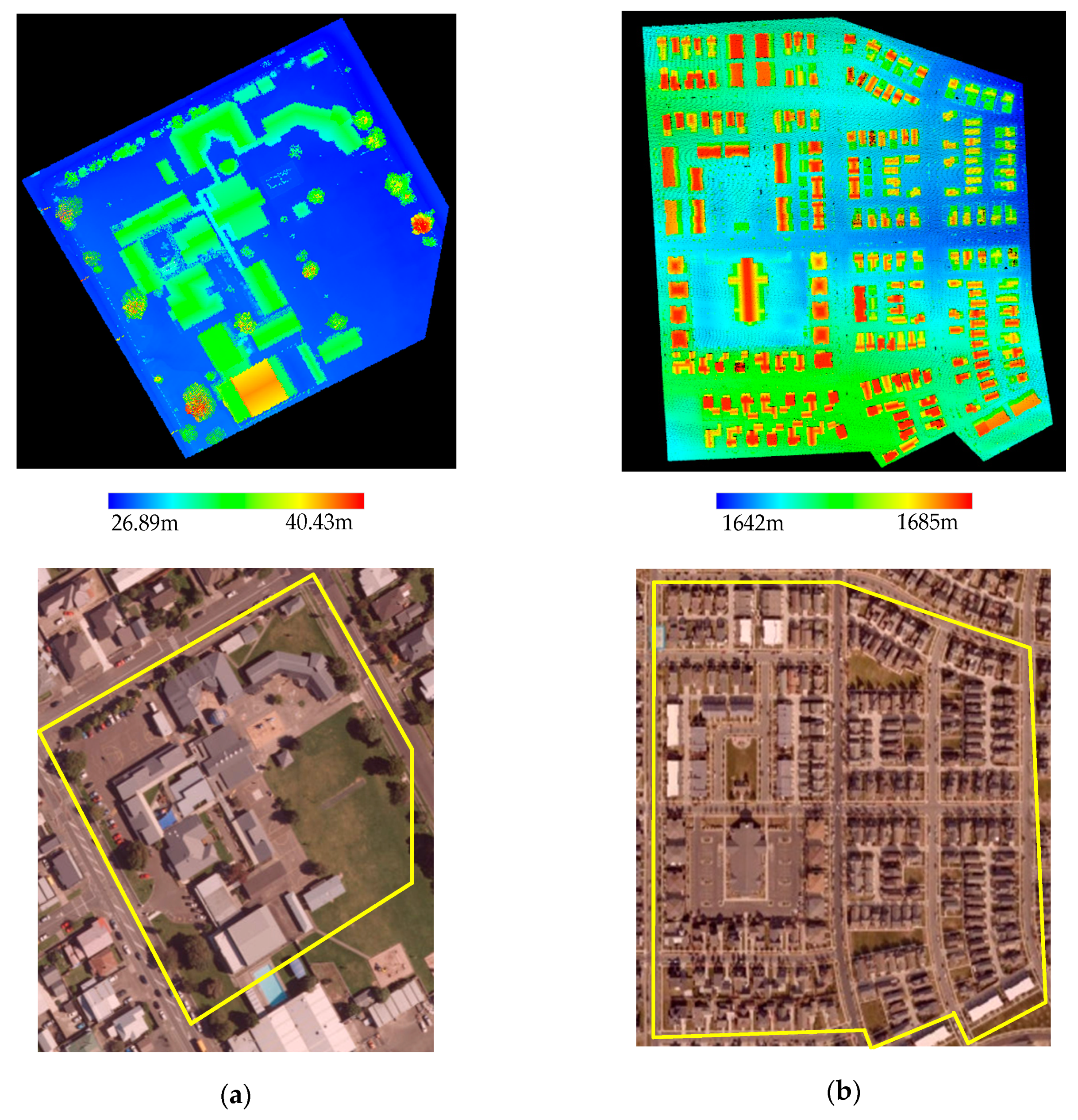
3.2. Experiments on Other Two LiDAR Datasets
3.2.1. Data Description
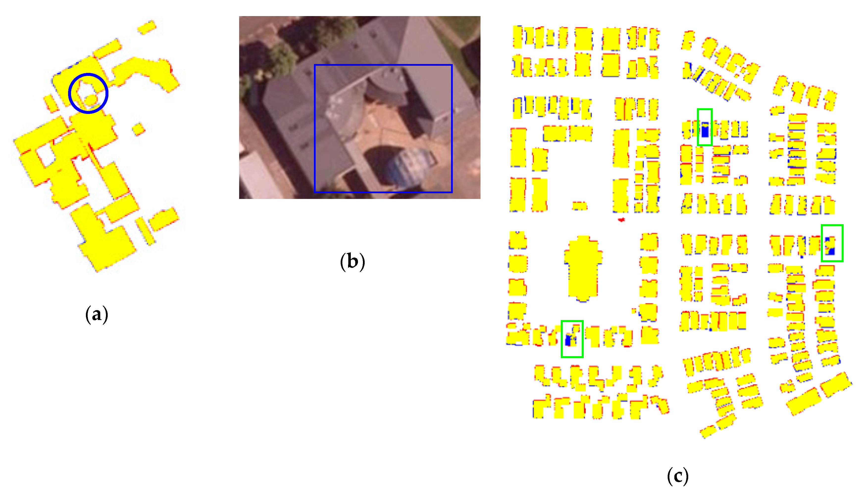
3.3.2. Results and Analysis
4. Discussion
4.1. Discussion of
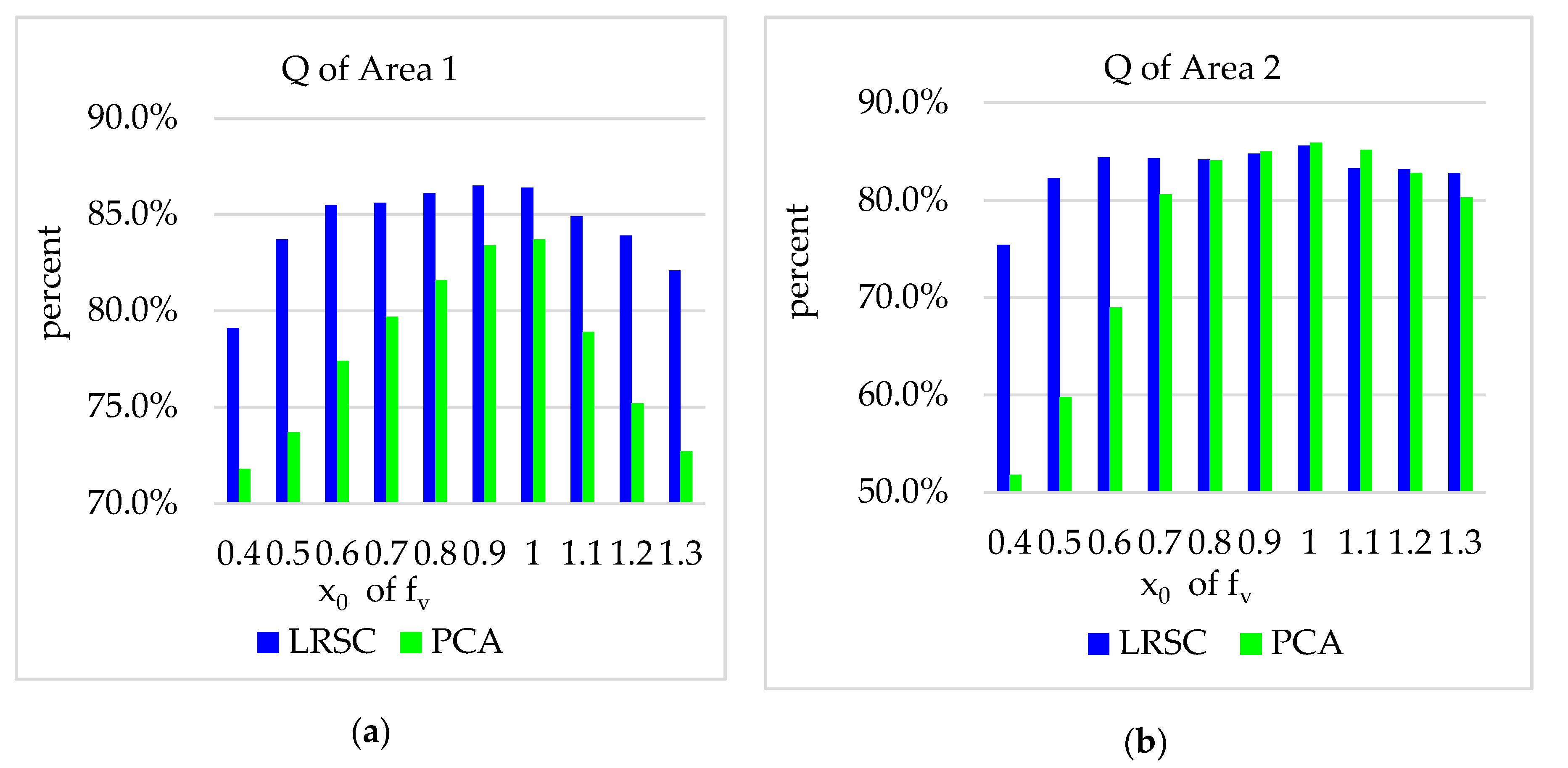
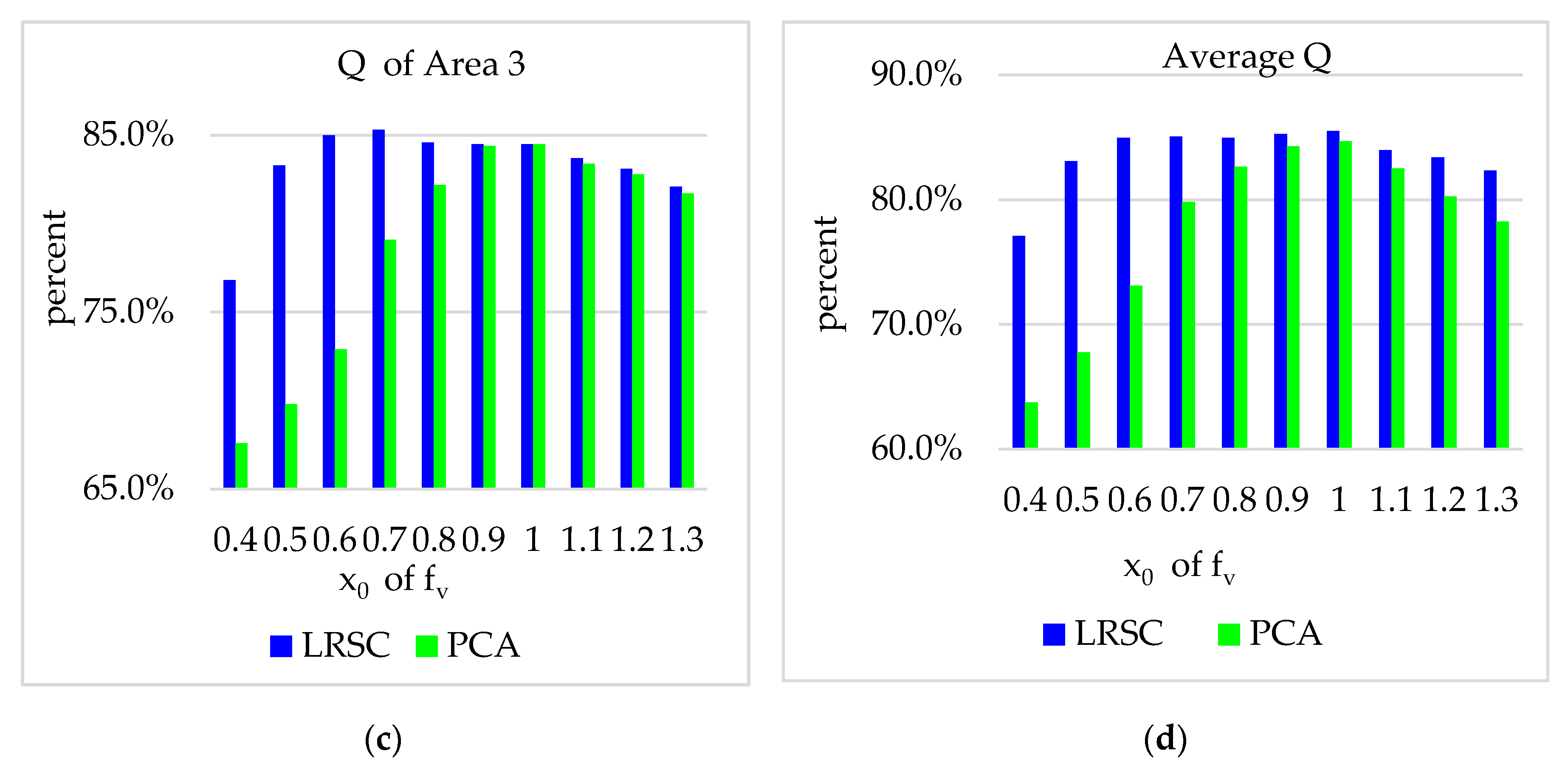
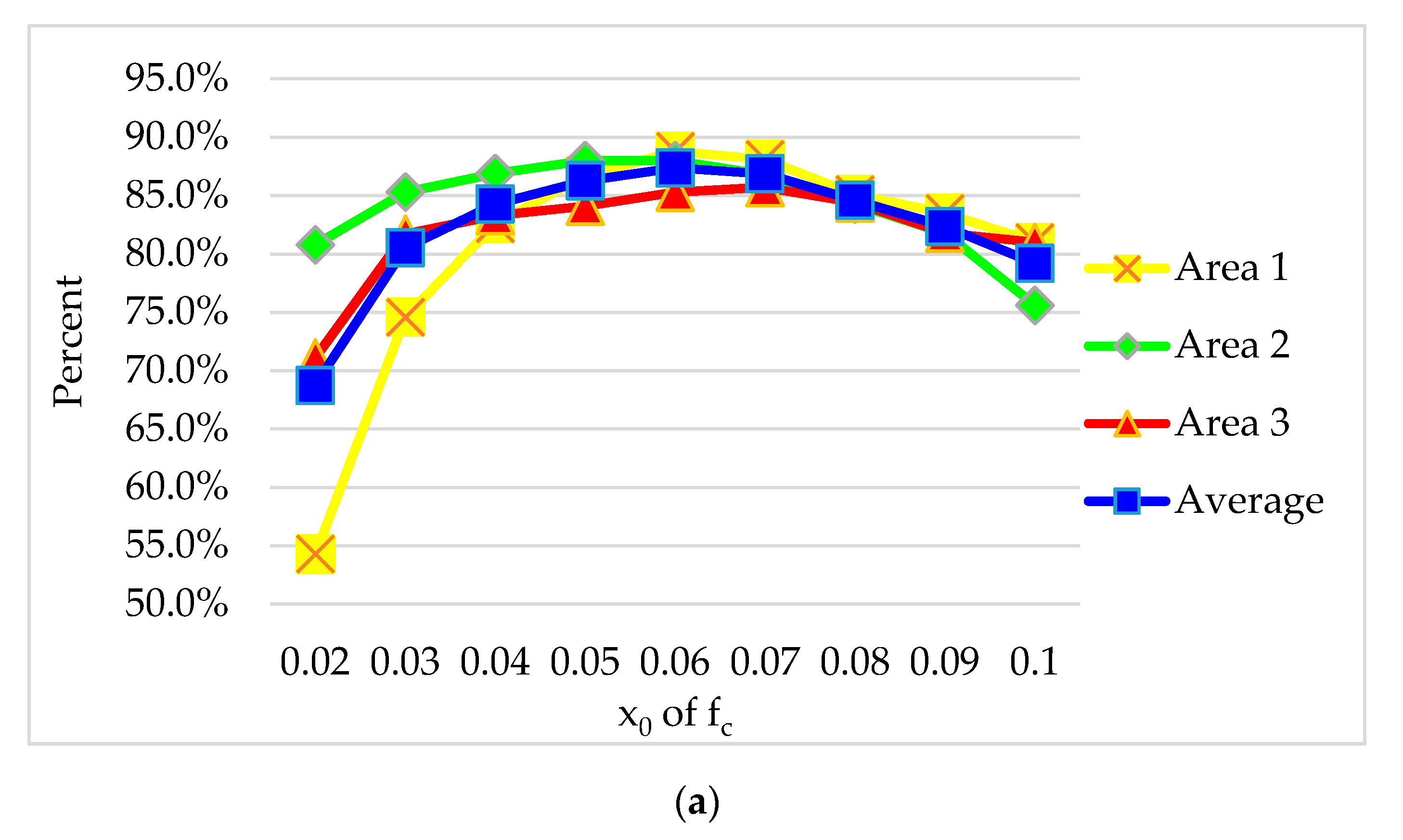
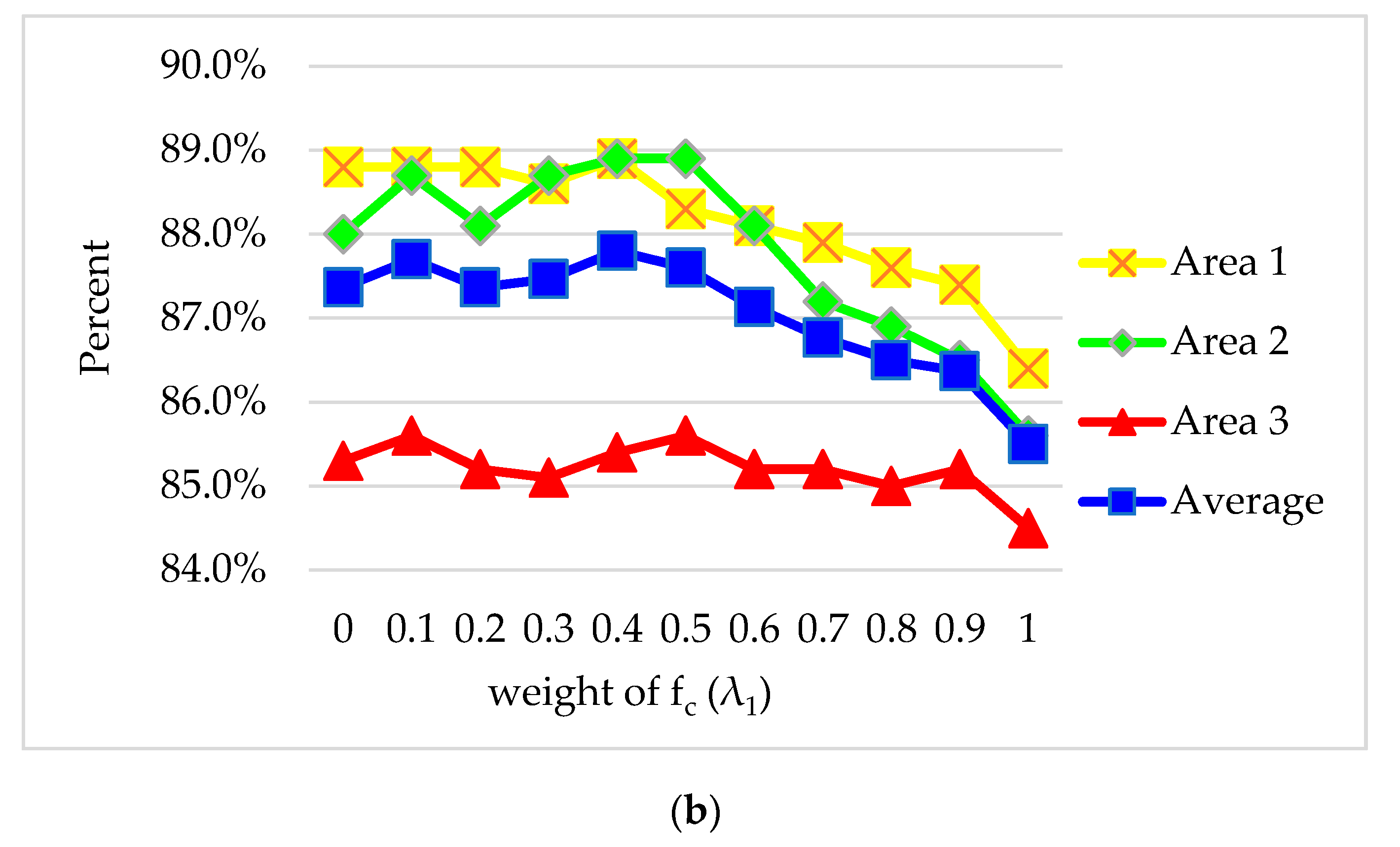
4.2. Discussion of Parameters Setting
4.3. Discussion of Running Time
5. Conclusions
Author Contributions
Funding
Acknowledgments
Conflicts of Interest
References
- Wang, R.; Peethambaran, J.; Chen, D. LiDAR point clouds to 3-D Urban Models: A review. IEEE J. Sel. Top. Appl. Earth Obs. Remote Sens. 2018, 11, 606–627. [Google Scholar] [CrossRef]
- Guo, L.; Luo, J.; Yuan, M.; Huang, Y.; Shen, H.; Li, T. The influence of urban planning factors on PM2.5 pollution exposure and implications: A case study in China based on remote sensing, LBS, and GIS data. Sci. Total Environ. 2019, 659, 1585–1596. [Google Scholar] [CrossRef] [PubMed]
- Janalipour, M.; Mohammadzadeh, A. A novel and automatic framework for producing building damage map using post-event LiDAR data. Int. J. Disaster Risk Reduct. 2019, 39, 1–13. [Google Scholar] [CrossRef]
- Peng, Z.; Gao, S.; Xiao, B.; Guo, S.; Yang, Y. CrowdGIS: Updating digital maps via mobile crowdsensing. IEEE Trans. Autom. Sci. Eng. 2017, 15, 369–380. [Google Scholar] [CrossRef]
- Zhou, Z.; Gong, J. Automated residential building detection from airborne LiDAR data with deep neural networks. Adv. Eng. Inform. 2018, 36, 229–241. [Google Scholar] [CrossRef]
- Chen, S.; Shi, W.; Zhou, M.; Zhang, M.; Chen, P. Automatic building extraction via adaptive iterative segmentation with LiDAR data and high spatial resolution imagery fusion. IEEE J. Sel. Top. Appl. Earth Obs. Remote Sens. 2020, 13, 2081–2095. [Google Scholar] [CrossRef]
- Mallet, C.; Bretar, F.; Roux, M.; Soergel, U.; Heipke, C. Relevance assessment of full-waveform lidar data for urban area classification. ISPRS J. Photogramm. Remote Sens. 2011, 66, S71–S84. [Google Scholar] [CrossRef]
- Donoghue, D.N.M.; Watt, P.J.; Cox, N.J.; Wilson, J. Remote sensing of species mixtures in conifer plantations using LiDAR height and intensity data. Remote Sens. 2007, 110, 509–522. [Google Scholar] [CrossRef]
- Salimzadeh, N.; Hammad, A. High-level framework for GIS-based optimization of building photovoltaic potential at urban scale using BIM and LiDAR. In Proceedings of the International Conference on Sustainable Infrastructure, New York, NY, USA, 26–28 October 2017; pp. 123–134. [Google Scholar] [CrossRef]
- Awrangjeb, M.; Zhang, C.; Fraser, C. Automatic extraction of building roofs using LIDAR data and multispectral imagery. ISPRS J. Photogramm. Remote Sens. 2013, 83, 1–18. [Google Scholar] [CrossRef] [Green Version]
- Awrangjeb, M.; Fraser, C. Automatic segmentation of raw LiDAR data for extraction of building roofs. Remote Sens. 2014, 6, 3716–3751. [Google Scholar] [CrossRef] [Green Version]
- Du, S.; Zhang, Y.; Zou, Z.; Xu, S.; He, X.; Chen, S. Automatic building extraction from LiDAR data fusion of point and grid-based features. ISPRS J. Photogramm. Remote Sens. 2017, 130, 294–307. [Google Scholar] [CrossRef]
- Ni, H.; Lin, X.; Zhang, J. Classification of ALS point cloud with improved point cloud segmentation and random forests. Remote Sens. 2017, 9, 288. [Google Scholar] [CrossRef] [Green Version]
- Vosselman, G.; Coenen, M.; Rottensteiner, F. Contextual segment-based classification of airborne laser scanner data. ISPRS J. Photogramm. Remote Sens. 2017, 128, 354–371. [Google Scholar] [CrossRef]
- Guo, B.; Huang, X.; Zhang, F.; Sohn, G. Classification of airborne laser scanning data using JointBoost. ISPRS J. Photogramm. Remote Sens. 2015, 100, 71–83. [Google Scholar] [CrossRef]
- Zhang, J.; Lin, X.; Ning, X. SVM-based classification of segmented airborne LiDAR point clouds in urban areas. Remote Sens. 2013, 5, 3749–3775. [Google Scholar] [CrossRef] [Green Version]
- Breiman, L. Random forests. Mach. Learn. 2001, 45, 5–32. [Google Scholar] [CrossRef] [Green Version]
- Moon, T.K. The expectation-maximization algorithm. IEEE Signal. Process. Mag. 1996, 13, 47–60. [Google Scholar] [CrossRef]
- Torlay, L.; Perrone-Bertolotti, M.; Thomas, E.; Baciu, M. Machine learning–XGBoost analysis of language networks to classify patients with epilepsy. Brain Inform. 2017, 4, 1–11. [Google Scholar] [CrossRef]
- Zhang, Z.; Zhang, L.; Tong, X.; Mathiopoulos, T.; Guo, B.; Huang, X.; Wang, Z.; Wang, Y. A multilevel point-cluster-based discriminative feature for ALS point cloud classification. IEEE Trans. Geosci. Remote Sens. 2016, 54, 3309–3321. [Google Scholar] [CrossRef]
- Weinmann, M.; Jutzi, B.; Mallet, C. Semantic 3D scene interpretation: A framework combining optimal neighborhood size selection with relevant features. ISPRS Ann. Photogramm. Remote Sens. Spat. Inf. Sci. 2014, 2, 181–188. [Google Scholar] [CrossRef] [Green Version]
- Wang, C.; Shu, Q.; Wang, X.; Guo, B.; Liu, P.; Li, Q. A random forest classifier based on pixel comparison features for urban LiDAR data. ISPRS J. Photogramm. Remote Sens. 2019, 148, 75–86. [Google Scholar] [CrossRef]
- Huang, R.; Yang, B.; Liang, F.; Dai, W.; Li, J.; Tian, M.; Xu, W. A top-down strategy for buildings extraction from complex urban scenes using airborne LiDAR point clouds. Infrared Phys. Technol. 2018, 92, 203–218. [Google Scholar] [CrossRef]
- Wang, Y.; Jiang, T.; Yu, M.; Tao, S.; Sun, J.; Liu, S. Semantic-based building extraction from LiDAR point clouds using contexts and optimization in complex environment. Sensors 2020, 20, 3386. [Google Scholar] [CrossRef] [PubMed]
- Dong, W.; Lan, J.; Liang, S.; Yao, W.; Zhang, Z. Selection of LiDAR geometric features with adaptive neighborhood size for urban land cover classification. Int. J. Appl. Earth Obs. Geoinf. 2017, 60, 99–110. [Google Scholar] [CrossRef]
- Han, W.; Wang, R.; Huang, D.; Xu, C. Large-Scale ALS data semantic classification integrating location-context-semantics cues by higher-order CRF. Sensors 2020, 20, 1700. [Google Scholar] [CrossRef] [Green Version]
- Cai, Z.; Ma, H.; Zhang, L. Feature selection for airborne LiDAR data filtering: A mutual information method with Parzon window optimization. GIsci. Remote Sens. 2020, 57, 323–337. [Google Scholar] [CrossRef]
- Vo, A.V.; Truong-Hong, L.; Laefer, D.F.; Bertolotto, M. Octree-Based region growing for point cloud segmentation. ISPRS J. Photogramm. Remote Sens. 2015, 104, 88–100. [Google Scholar] [CrossRef]
- Xu, Y.; Yao, W.; Hoegner, L.; Stilla, U. Segmentation of building roofs from airborne LiDAR point clouds using robust voxel-based region growing. Remote Sens. Lett. 2017, 8, 1062–1071. [Google Scholar] [CrossRef]
- Awrangjeb, M.; Lu, G.; Fraser, C. Automatic building extraction from LiDAR data covering complex urban scenes. Int. Arch. Photogramm. Remote Sens. Spat. Inf. Sci. 2014, 40, 25–32. [Google Scholar] [CrossRef] [Green Version]
- Wang, Y.; Sun, Y.; Liu, Z.; Sarma, S.E.; Bronstein, M.M.; Solomon, J.M. Dynamic graph cnn for learning on point clouds. ACM Trans. Graph. 2019, 38, 1–12. [Google Scholar] [CrossRef] [Green Version]
- Hu, X.; Yuan, Y. Deep-Learning-Based classification for DTM extraction from ALS point cloud. Remote Sens. 2016, 8, 730. [Google Scholar] [CrossRef] [Green Version]
- Yao, X.; Guo, J.; Hu, J.; Cao, Q. Using deep learning in semantic classification for point cloud data. IEEE Access 2019, 7, 37121–37130. [Google Scholar] [CrossRef]
- Verma, V.; Kumar, R.; Hsu, S. 3D building detection and modeling from aerial LiDAR data. In Proceedings of the 2006 IEEE Computer Society Conference on Computer Vision and Pattern Recognition, IEEE Computer Society, Washington, DC, USA, 17–22 June 2006; pp. 2213–2220. [Google Scholar] [CrossRef]
- Tarsha-Kurdi, F.; Landes, T.; Grussenmeyer, P. Hough-Transform and extended RANSAC algorithms for automatic detection of 3D building roof planes from LiDAR data. Int. Arch. Photogramm. Remote Sens. 2007, 66, 124–132. [Google Scholar] [CrossRef]
- Borrmann, D.; Elseberg, J.; Lingemann, K.; Nüchte, A. The 3d hough transform for plane detection in point clouds: A review and a new accumulator design. 3D Res. 2011, 2, 1–13. [Google Scholar] [CrossRef]
- Cai, Z.; Ma, H.; Zhang, L. A Building detection method based on semi-suppressed fuzzy C-means and restricted region growing using airborne LiDAR. Remote Sens. 2019, 11, 848. [Google Scholar] [CrossRef] [Green Version]
- Adhikari, S.K.; Sing, J.K.; Basu, D.K.; Nasipuri, M. Conditional spatial fuzzy C-means clustering algorithm for segmentation of MRI images. Appl. Soft Comput. 2015, 34, 758–769. [Google Scholar] [CrossRef]
- Meng, X.; Wang, L.; Currit, N. Morphology-Based building detection from airborne LIDAR data. Photogramm. Eng. Remote Sens. 2009, 75, 437–442. [Google Scholar] [CrossRef]
- Cheng, L.; Zhao, W.; Han, P.; Zhang, W.; Shan, J.; Liu, Y. Building region derivation from LiDAR data using a reversed iterative mathematic morphological algorithm. Opt. Commun. 2013, 286, 244–250. [Google Scholar] [CrossRef]
- Gerke, M.; Xiao, J. Fusion of airborne laserscanning point clouds and images for supervised and unsupervised scene classification. ISPRS J. Photogramm. Remote Sens. 2014, 87, 78–92. [Google Scholar] [CrossRef]
- Rusu, R.B.; Cousins, S. 3D is here: Point cloud library. In Proceeding of the IEEE International Conference on Robotics and Automation, Shanghai, China, 9–13 May 2011; pp. 1–4. [Google Scholar] [CrossRef] [Green Version]
- Rusu, R.B.; Marton, Z.C.; Blodow, N.; Dolha, M.; Beetz, M. Towards 3D point cloud based object maps for household environments. Rob. Auton. Syst. 2008, 56, 927–941. [Google Scholar] [CrossRef]
- Ma, H.; Zhou, W.; Zhang, L. DEM refinement by low vegetation removal based on the combination of fullwaveform data and progressive TIN densification. ISPRS J. Photogramm. Remote Sens. 2018, 146, 260–271. [Google Scholar] [CrossRef]
- Axelsson, P. Processing of laser scanner data-algorithms and applications. ISPRS J. Photogramm. Remote Sens. 1999, 54, 138–147. [Google Scholar] [CrossRef]
- Liu, K.; Ma, H.; Zhang, L.; Cai, Z.; Ma, H. Strip adjustment of airborne LiDAR data in urban scenes using planar features by the minimum hausdorff distance. Sensors 2019, 19, 5131. [Google Scholar] [CrossRef] [PubMed] [Green Version]
- Blomley, R.; Jutzi, B.; Weinmann, M. Classification of airborne laser scanning data using geometric, multi-scale features and different neighborhood types. ISPRS Ann. Photogramm. Remote Sens. Spat. Inf. Sci. 2016, 3, 169–176. [Google Scholar] [CrossRef]
- Zhang, J.; Cao, J.; Liu, X.; Wang, J.; Liu, J.; Shi, X. Point cloud normal estimation via low-rank subspace clustering. Comput. Graph. 2013, 37, 697–706. [Google Scholar] [CrossRef]
- ISPRS. Available online: http://www2.isprs.org/commissions/comm3/wg4/tests.html (accessed on 22 August 2020).
- Li, Y.; Tong, G.; Du, X.; Yang, X.; Zhang, J.; Yang, L. A single point-based multilevel features fusion and pyramid neighborhood optimization method for ALS point cloud classification. Appl. Sci. 2019, 9, 951. [Google Scholar] [CrossRef] [Green Version]
- Gilani, S.A.N.; Awrangjeb, M.; Lu, G. Segmentation of airborne point cloud data for automatic building roof extraction. GIsci. Remote Sens. 2018, 55, 63–89. [Google Scholar] [CrossRef] [Green Version]
- Delong, A.; Osokin, A.; Isack, H.N.; Boykov, Y. Fast approximate energy minimization with label costs. Int. J. Comput. Vis. 2012, 96, 1–27. [Google Scholar] [CrossRef]
- Ural, S.; Shan, J. Min-Cut based segmentation of airborne LiDAR point clouds. Int. Arch. Photogramm. Remote Sens. Spat. Inf. Sci. 2012, 39, 167–172. [Google Scholar] [CrossRef] [Green Version]
- Boykov, Y.; Kolmogorov, V. An experimental comparison of min-cut/max- flow algorithms for energy minimization in vision. IEEE Trans. Pattern Anal. Mach. Intell. 2004, 26, 1124–1137. [Google Scholar] [CrossRef] [Green Version]
- Li, W.; Wang, Y.; Du, J.; Lai, J. Synergistic integration of graph-cut and cloud model strategies for image segmentation. Neurocomputing 2017, 257, 37–46. [Google Scholar] [CrossRef]
- Guo, Y.; Akbulut, Y.; Şengür, A.; Xia, R.; Smarandache, F. An efficient image segmentation algorithm using neutrosophic graph cut. Symmetry 2017, 9, 185. [Google Scholar] [CrossRef] [Green Version]
- Reza, M.N.; Na, I.S.; Baek, S.W.; Lee, K.H. Rice yield estimation based on K-means clustering with graph-cut segmentation using low-altitude UAV images. Biosyst. Eng. 2019, 177, 109–121. [Google Scholar] [CrossRef]
- Sánchez-Lopera, J.; Lerma, J.L. Classification of lidar bare-earth points, buildings, vegetation, and small objects based on region growing and angular classifier. Int. J. Remote Sens. 2014, 35, 6955–6972. [Google Scholar] [CrossRef]
- Truong, L.T.; Nguyen, H.T.; Nguyen, H.D.; Vu, H.V. Pedestrian overpass use and its relationships with digital and social distractions, and overpass characteristics. Accid. Anal. Prev. 2019, 131, 234–238. [Google Scholar] [CrossRef]
- OpenTopography. Available online: https://portal.opentopography.org/datasetMetadata?otCollectionID=OT.022020.2193.2 (accessed on 22 August 2020). [CrossRef]
- OpenTopography. Available online: https://portal.opentopography.org/datasetMetadata?otCollectionID=OT.122014.26912.1 (accessed on 22 August 2020). [CrossRef]
- Ardila, J.P.; Tolpekin, V.A.; Bijker, W.; Stein, A. Markov-Random-Field-Based super-resolution mapping for identification of urban trees in VHR images. ISPRS J. Photogramm. Remote Sens. 2011, 66, 762–775. [Google Scholar] [CrossRef]
- Rutzinger, M.; Rottensteiner, F.; Pfeifer, N. A comparison of evaluation techniques for building extraction from airborne laser scanning. IEEE J. Sel. Top. Appl. Earth Obs. Remote Sens. 2009, 2, 11–20. [Google Scholar] [CrossRef]
- Ma, L.; Li, Y.; Li, J.; Zhong, Z.; Chapman, M. Generation of horizontally curved driving lines in HD maps using mobile laser scanning point clouds. IEEE J. Sel. Top. Appl. Earth Obs. Remote Sens. 2019, 12, 1572–1586. [Google Scholar] [CrossRef]
- Powers, D. Evaluation: From precision, recall and F-measure to ROC, informedness, markedness and correlation. J. Mach. Learn. Tech. 2011, 2, 37–63. [Google Scholar]
- Eesa, A.S.; Arabo, W.K. A normalization methods for backpropagation: A comparative study. Sci. J. Univ. Zakho 2017, 5, 319–323. [Google Scholar] [CrossRef]


| Test Case | Per-Area (%) | Per-Object (%) | Per-Object > 50 m2 (%) | |||||||||
|---|---|---|---|---|---|---|---|---|---|---|---|---|
| CP | CR | Q | CP | CR | Q | CP | CR | Q | ||||
| Area 1 | 97.1 | 91.4 | 88.9 | 94.2 | 83.8 | 96.9 | 81.6 | 89.9 | 100 | 100 | 100 | 100 |
| Area 2 | 95.4 | 92.9 | 88.9 | 94.1 | 85.7 | 100 | 85.7 | 92.3 | 100 | 100 | 100 | 100 |
| Area 3 | 94.1 | 90.2 | 85.4 | 92.1 | 83.9 | 100 | 83.9 | 91.2 | 97.4 | 100 | 97.4 | 98.7 |
| Average | 95.5 | 91.5 | 87.7 | 93.5 | 84.5 | 99.0 | 83.7 | 91.2 | 99.1 | 100 | 99.1 | 99.5 |
| Area 4 | 98.2 | 90.5 | 89.1 | 94.2 | 98.3 | 85.5 | 84.6 | 91.5 | 100 | 93.4 | 93.4 | 96.6 |
| Area 5 | 98.6 | 89.8 | 88.7 | 94.0 | 94.7 | 72.0 | 69.2 | 81.8 | 97.1 | 84.6 | 82.5 | 90.4 |
| Average | 98.4 | 90.2 | 88.9 | 94.1 | 96.5 | 78.8 | 76.7 | 86.6 | 98.6 | 89.0 | 88.0 | 93.5 |
| ID | Per-Area (%) | Per-Object (%) | Per-Object > 50 m2 (%) | |||||||||
|---|---|---|---|---|---|---|---|---|---|---|---|---|
| CP | CR | Q | CP | CR | Q | CP | CR | Q | ||||
| UMTA | 92.3 | 87.5 | 81.5 | 89.8 | 80.0 | 98.6 | 79.1 | 88.3 | 99.1 | 100.0 | 99.1 | 99.5 |
| UMTP | 92.4 | 86.0 | 80.3 | 89.1 | 80.9 | 95.8 | 78.1 | 87.7 | 98.8 | 97.2 | 96.0 | 98.0 |
| MON | 92.7 | 88.7 | 82.8 | 90.7 | 82.7 | 93.1 | 77.7 | 87.6 | 99.1 | 100.0 | 99.1 | 99.5 |
| VSK | 85.8 | 98.4 | 84.6 | 91.7 | 79.7 | 100.0 | 79.7 | 88.7 | 97.9 | 100.0 | 97.9 | 98.9 |
| WHUY1 | 87.3 | 91.6 | 80.8 | 89.4 | 77.6 | 98.1 | 76.5 | 86.7 | 97.4 | 97.9 | 95.4 | 97.6 |
| WHUY2 | 89.7 | 90.9 | 82.3 | 90.3 | 83.0 | 97.5 | 81.3 | 89.7 | 99.1 | 98.0 | 97.2 | 98.5 |
| HANC1 | 91.5 | 92.5 | 85.2 | 92.0 | 81.5 | 72.7 | 62.4 | 76.8 | 100.0 | 95.8 | 95.8 | 97.9 |
| HANC2 | 90.2 | 93.2 | 84.6 | 91.7 | 85.1 | 69.6 | 61.9 | 76.6 | 100.0 | 100.0 | 100.0 | 100.0 |
| MAR1 | 87.0 | 97.1 | 84.8 | 91.8 | 78.2 | 96.2 | 75.7 | 86.3 | 99.1 | 100.0 | 99.1 | 99.5 |
| MAR2 | 89.7 | 95.2 | 85.8 | 92.4 | 80.6 | 93.7 | 76.5 | 86.7 | 99.1 | 98.9 | 98.0 | 99.0 |
| TON | 77.7 | 97.7 | 76.3 | 86.6 | 67.5 | 98.9 | 66.9 | 80.2 | 92.7 | 98.8 | 91.6 | 95.7 |
| HANC3 | 91.3 | 95.9 | 87.8 | 93.5 | 85.4 | 82.2 | 71.7 | 83.8 | 100.0 | 98.9 | 98.9 | 99.4 |
| WHU_QC | 85.8 | 98.7 | 84.8 | 91.8 | 80.9 | 99.0 | 80.3 | 89.0 | 96.8 | 100.0 | 96.8 | 98.4 |
| MON2 | 87.6 | 91 | 80.6 | 89.3 | 86.3 | 93.9 | 81.6 | 89.9 | 99.1 | 100.0 | 99.1 | 99.5 |
| WHU_YD | 89.8 | 98.6 | 88.6 | 94.0 | 87.8 | 99.3 | 87.3 | 93.2 | 99.1 | 100.0 | 99.1 | 99.5 |
| MON4 | 94.3 | 82.9 | 79.0 | 88.2 | 83.9 | 93.8 | 79.3 | 88.6 | 99.1 | 100.0 | 99.1 | 99.5 |
| MON5 | 89.9 | 90.3 | 82 | 90.1 | 87.2 | 96.3 | 84.4 | 91.5 | 99.1 | 100.0 | 99.1 | 99.5 |
| [12] | 94.0 | 94.9 | 89.5 | 94.4 | 83.3 | 100.0 | 83.3 | 90.9 | 100.0 | 100.0 | 100.0 | 100.0 |
| [23] | 89.8 | 98.6 | 88.6 | 94.0 | 87.8 | 99.3 | 87.3 | 93.2 | - | - | - | - |
| [37] | 93.4 | 95.8 | 89.6 | 94.6 | - | - | - | - | - | - | - | - |
| WHU_TQ | 95.5 | 91.5 | 87.7 | 93.5 | 84.5 | 99.0 | 83.7 | 91.2 | 99.1 | 100.0 | 99.1 | 99.5 |
| ID | Per-Area (%) | Per-Object (%) | Per-Object > 50 m2 (%) | |||||||||
|---|---|---|---|---|---|---|---|---|---|---|---|---|
| CP | CR | Q | CP | CR | Q | CP | CR | Q | ||||
| TUM | 85.1 | 80.6 | 70.6 | 82.7 | 83.9 | 90.3 | 76.9 | 87.0 | 88.2 | 92.5 | 82.3 | 90.3 |
| MAR1 | 96.1 | 92.1 | 88.7 | 94.0 | 98.7 | 86.8 | 85.8 | 92.4 | 98.6 | 87.6 | 86.5 | 92.8 |
| WHUY2 | 94.3 | 91.3 | 86.5 | 92.7 | 90.4 | 95.8 | 87.0 | 93.0 | 94.8 | 95.8 | 91.0 | 95.3 |
| ITCM | 76.9 | 87.5 | 69.2 | 81.8 | 86.5 | 21.7 | 20.9 | 34.6 | 89.7 | 70.5 | 65.2 | 78.9 |
| ITCR | 75.0 | 94.5 | 71.9 | 83.6 | 79.6 | 43.5 | 39.1 | 56.2 | 83.8 | 91.8 | 77.9 | 87.6 |
| MAR2 | 94.0 | 94.3 | 88.9 | 94.1 | 91.3 | 91.9 | 84.5 | 91.6 | 95.7 | 96.8 | 92.8 | 96.2 |
| MON2 | 95.9 | 92.2 | 88.7 | 94.0 | 93.4 | 81.1 | 76.7 | 86.8 | 95.7 | 94.5 | 90.7 | 95.1 |
| Z_GIS | 91.7 | 90.3 | 83.4 | 91.0 | 95.7 | 86.4 | 83.1 | 90.8 | 96.3 | 87.3 | 84.4 | 91.5 |
| WHU_YD | 95.8 | 94.6 | 90.8 | 95.2 | 91.3 | 95.4 | 87.4 | 93.3 | 95.7 | 95.4 | 91.4 | 95.5 |
| HKP | 97.6 | 92.7 | 90.6 | 95.1 | 93.9 | 90.4 | 85.4 | 92.1 | 95.7 | 90.4 | 86.9 | 93.0 |
| [23] | 95.8 | 94.7 | 90.8 | 95.2 | 91.3 | 95.4 | 87.5 | 93.3 | - | - | - | - |
| WHU_TQ | 98.4 | 90.2 | 88.9 | 94.1 | 96.5 | 78.8 | 76.7 | 86.6 | 98.6 | 89.0 | 88.0 | 93.5 |
| Precision (Per-Area) | CP (%) | CR (%) | Q (%) | ||
|---|---|---|---|---|---|
| Data | |||||
| New Zealand dataset Utah dataset | 98.4 | 94.7 | 93.2 | 96.5 | |
| 95.3 | 92.3 | 88.3 | 93.8 | ||
| Area ID | Area 1 | Area 2 | Area 3 | Area 4 | Area 5 | New Zealand Dataset | Utah Dataset | |
|---|---|---|---|---|---|---|---|---|
| Item | ||||||||
| 14 | 18 | 20 | 357 | 307 | 70 | 127 | ||
| 23 | 51 | 61 | 4831 | 4642 | 653 | 2239 | ||
| 37 | 69 | 81 | 5188 | 4949 | 723 | 2366 | ||
© 2020 by the authors. Licensee MDPI, Basel, Switzerland. This article is an open access article distributed under the terms and conditions of the Creative Commons Attribution (CC BY) license (http://creativecommons.org/licenses/by/4.0/).
Share and Cite
Liu, K.; Ma, H.; Ma, H.; Cai, Z.; Zhang, L. Building Extraction from Airborne LiDAR Data Based on Min-Cut and Improved Post-Processing. Remote Sens. 2020, 12, 2849. https://doi.org/10.3390/rs12172849
Liu K, Ma H, Ma H, Cai Z, Zhang L. Building Extraction from Airborne LiDAR Data Based on Min-Cut and Improved Post-Processing. Remote Sensing. 2020; 12(17):2849. https://doi.org/10.3390/rs12172849
Chicago/Turabian StyleLiu, Ke, Hongchao Ma, Haichi Ma, Zhan Cai, and Liang Zhang. 2020. "Building Extraction from Airborne LiDAR Data Based on Min-Cut and Improved Post-Processing" Remote Sensing 12, no. 17: 2849. https://doi.org/10.3390/rs12172849