Illuminating the Spatio-Temporal Evolution of the 2008–2009 Qaidam Earthquake Sequence with the Joint Use of Insar Time Series and Teleseismic Data

Abstract

Inferring the geometry and evolution of an earthquake sequence is crucial to understand how fault systems are segmented and interact. However, structural geological models are often poorly constrained in remote areas and fault inference is an ill-posed problem with a reliability that depends on many factors. Here, we investigate the geometry of the Mw 6.3 2008 and 2009 Qaidam earthquakes, in northeast Tibet, by combining InSAR time series and teleseismic data. We conduct a multi-array back-projection analysis from broadband teleseismic data and process three overlapping Envisat tracks covering the two earthquakes to extract the spatio-temporal evolution of seismic ruptures. We then integrate both geodetic and seismological data into a self-consistent kinematic model of the earthquake sequence. Our results constrain the depth and along-strike segmentation of the thrust-faulting sequence. The 2008 earthquake ruptured a ∼32° north-dipping fault that roots under the Olongbulak pop-up structure at ∼12 km depth and fault slip evolved post-seismically in a downdip direction. The 2009 earthquake ruptured three south-dipping high-angle thrusts and propagated from ∼9 km depth to the surface and bilaterally along the south-dipping segmented 55–75° high-angle faults of the Olonbulak pop-up structure that displace basin deformed sedimentary sequences above Paleozoic bedrock. Our analysis reveals that the inclusion of the post-seismic afterslip into modelling is beneficial in the determination of fault geometry, while teleseismic back-projection appears to be a robust tool for identifying rupture segmentation for moderate-sized earthquakes. These findings support the hypothesis that the Qilian Shan is expanding southward along a low-angle décollement that partitions the oblique convergence along multiple flower and pop-up structures.

1. Introduction

Inferring earthquake slip distributions is useful for understanding the spatial and temporal evolution of crustal strain, in order to investigate how faults are segmented and interact, and to study the relationship of an earthquake with the structural tectonics of an area. However, earthquake fault inversion is an ill-posed problem. Its solution is limited by data resolution, model simplifications and biases, the non-linearity between the data and the unknown parameters, the impact of the topography and lateral variations of lithology, and/or significant dependence between inverted parameters e.g., [1,2,3,4]. The reliability of any earthquake fault inversion depends on many factors, including the segmentation and size of the rupture, the quality of the data, the uncertainties in the subsurface model, the chosen optimisation method to infer earthquake fault parameters, and the a priori inferences of the earthquake geometry or mechanisms. For these reasons, different research groups often find different solutions for the same earthquake [5].

One way to reduce the non-uniqueness of an inversion and the impact of data errors is to combine several data sets with different characteristics (e.g., space-based imaging, seismic data, pixel offsets, tsunami records) e.g., [6,7,8,9]. In particular, several studies e.g., [4,10,11,12,13] have shown the benefit of complementing the high spatial resolution of near-field geodetic observations with the high temporal resolution of far-field seismic waveforms. Seismic waveforms carry information about the rupture onset time, its spatio-temporal evolution and duration, as well as the fault mechanism and seismic moment. Near-field surface data provide constraints on the fault location and mechanism, the amount of slip, and the extension of the rupture. Another way to limit biases in the inversion is to account for data and model parameter uncertainties due to the data noise and the imperfect knowledge of the medium through data weighting e.g., [1,14,15,16], and to rigorously propagate errors through optimisation algorithms, such as with un-regularised Bayesian optimisation frameworks e.g., [2,9,13,17,18,19,20]

Differential Interferometric Synthetic Aperture Radar (DInSAR) detects surface displacements in the line-of-sight (LOS) direction between satellite acquisitions before and after an earthquake, and it is commonly used to infer earthquake fault parameters due to its high spatial resolution e.g., [21,22,23,24,25,26]. Despite the large benefits that are brought by the measurement of the surface displacements across wide swaths, DInSAR is also polluted by changes of atmospheric conditions between the two acquisitions, associated with the turbulent and stratified components of the atmosphere and the electron content in the ionosphere [27,28,29]. In addition, due to the revisit time of the satellites of more than a few days, most inferred earthquake fault models based solely on DInSAR observations are biased by early post-seismic displacement signals. Apart from few studies that account for early post-seismic signals e.g., [30,31], most of the fault inferences neglect the contribution of early post-seismic deformation in the inverse problems with the consequences that it is attributed to the co-seismic rupture. However, since the first surface displacement image of an earthquake following the 1992 Landers earthquake [32], numerous advances in the DInSAR technique have been made to derive multi-temporal time series (TS) of ground displacements by processing multiple SAR acquisitions. This increases the number of locations where displacement can be measured and reduces associated errors e.g., [33,34,35]. Advances have also been made in reducing atmospheric contributions by the use of atmospheric models e.g., [28,36,37], empirical methods e.g., [35,38,39,40,41,42] or by data stacking and TS analysis e.g., [30,43,44,45]. The latter is beneficial to derive the cumulative surface displacements (contrary to single interferograms) and separates the various inter-, co- and post-seismic phases of the seismic cycle. In addition, TS analysis allows researchers to check the consistency of each interferogram within the network, increases the signal-to-noise ratio via data redundancy and attenuates the effects of turbulent atmospheric noise by smoothing of the TS. Recent developments in InSAR methodologies as well as the new generation of SAR satellites (Sentinel-1, ALOS-2) with shorter revisit times and systematic acquisitions in both ascending and descending geometries, therefore, raise queries about the prospects of multi-temporal InSAR TS for subsurface fault slip inferences.

The North Qaidam thrust (NQT) system is located at the southernmost part of the Qilian Shan-Nan Shan and is marked by recent active seismicity within the Olongbulak ranges (Figure 1). The ∼16 km deep 10 November 2008 and the ∼5 km deep 28 August 2009 Haixi $M_w$ 6.3 earthquakes occurred in close proximity (∼15 km) to each other within the Olongbulak Shan and were followed by a period of increased rate of seismicity in the region [46,47]. The 2009 earthquake was followed by a M_w 5.4 and a M_w 5.6 aftershock one and two days, respectively, after the main-shock, as many as 34 M_w > 4 aftershocks within a month (USGS), and time-dependent after-slip of similar pattern to the co-seismic slip [48,49,50,51]. The two earthquakes represent particular examples of two ∼$M_w$ 6 earthquakes that occurred nearby in space and time, highlighting the need to constrain both along-depth and along-strike segmentation of thrusting events to better quantify seismic hazards [46]. Their segmentations and geometries also need to be placed in the context of the regional tectonic as the deformation style of the northeastern part of the Tibetan plateau is at the heart of the debates about its dynamic evolution. In a first class of deformation models, Burchfiel et al., 1989 [52] first postulated a basement décollement fault in the middle crust of the Qaidam basin that connect to the Qilian Shan-Nan Shan thrust belts in the north, absorbing progressively the left-lateral slip on the Altyn-Tagh Fault (Figure 1). Subsequently, Metivier et al., 1998 [53], Meyer et al., 1998 [54] and Tapponnier et al., 2001 [55] suggested that the Qaidam basin may have been trapped of the surrounding reliefs in the middle-late Miocene as a result of the northward stepwise jumping of the intra-continental deformation. This first class of model proposes that the oblique convergence between the India-Eurasia collision is absorbed by crustal thickening along the major Kunlun or Qilian Shan suture zones, where strike-slip and thrust faults root at depth to extrude laterally and partition vertically the deformation causing mountain uplift on localised ranges (Figure S1a). Conversely, Dupont et al., 2004 [56], Yin et al., 2008a [57], and Bush et al., 2016 [58] suggested a plausible and simultaneous early Eocene onset of the Kunlun and Qilian ranges. This second class of model suggests that the strain from the India-Asia collision was rapidly transmitted to the northern edge of the modern Tibetan Plateau via preexisting and complex zones of weaknesses created during pre-Cenozoic [57,59,60] or via homogeneous deformation driven by mantle or crustal flow [61,62,63] (Figure S1b). Those model contradictions leave thus open the debate on the geometry of the NQT at depth and its possible relations with the Qilian ranges, to the north [55,59].

The study of these earthquakes is also challenging from a methodological point of view. First, because of the deeper source of the 2008 earthquake, the data can be explained by conjugate south-dipping or north-dipping planes, as illustrated by the various solutions found by different authors [46,47,48]. Secondly, the larger gradients and more complex surface displacement patterns of the 2009 earthquake, in comparison to the 2008 earthquake, suggest a segmented and shallow rupture. These surface displacement features have been explained by varying numbers of fault segments in the literature [46,48,65], and this earthquake sequence, therefore, also represents a good case study to evaluate the level of complexity that is required in a fault model to explain the data.

In this study, we investigate the spatio-temporal evolution of the 2008 and 2009 earthquakes using seismological back-projection analysis and three overlapping InSAR time series (TS) data of the Envisat satellite covering the two earthquakes. We then integrate both geodetic and seismological data into a self-consistent fault model. The goals of this study are multi-folds. We first investigate the fitness of back-projection to describe the rupture characteristics of moderate-size earthquakes. We then inspect the benefits of an InSAR TS analysis approach for earthquake fault modelling and discuss the improved signal to noise ratio of such data sets in comparison to traditional co-seismic interferograms, as well as the additional constraints that are offered by the extracted post-seismic surface displacements from InSAR time-series data. We finally integrate our fault characteristic estimations to the local tectonic context to propose a structural model of the Olongbulak ranges.

2. Materials and Methods

2.1. Seismic Back-Projection Source Imaging

Time-domain seismic back-projection images the spatio-temporal evolution of earthquakes by mapping the location of coherent seismic wave emissions recorded at a seismic network e.g., [66,67,68,69]. It relies on constructive and destructive stacking of seismic waveforms. In comparison to kinematic fault inversion, it has the advantage of requiring no assumption of the fault geometry, and is, therefore, a useful complement to inverse modelling. The only model assumptions required are the travel times derived from a one-dimensional (1-D) Earth velocity model.

2.1.1. Data and Station Clustering

We first download all available broadband records from the international web service (FDSNWS) Geofon and IRIS [70,71], for the 2008 and 2009 Qaidam earthquakes. We consider waveforms from broadband stations between 20° and 93° distance from the source and only use stations that recorded both earthquakes (Figure S2). We cluster the available stations using the k-means algorithm into many small virtual arrays (minimum number of five stations). Virtual arrays are formed assuming a minimum number of stations and a maximum aperture up to 3.5°. The use of many small virtual arrays has the advantage of minimising the effect of velocity differences between stations in an array as well as the effect of radiation patterns and source directivity [72].

2.1.2. Muti-Array Back-Projection Method

We carry out the back-projection for point locations on a horizontal grid. We perform the back-projection separately for high-frequencies (HF) and low-frequencies (LF), in order to explore areas with changes of frequency content over time, which can indicate changes in slip velocity/acceleration [73] or rupture initiation points [74]. We perform the back-projection on moving time windows of 2 s steps and 10 s length for HF and of 8 s steps and 26 s length for LF. We bandpass-filter for the HF back-projection between the earthquake corner frequency ($2/T_r$, with $T_r$ being the reported gCMT rupture duration [64]) and 1.5 Hz. For the LF back-projection we bandpass-filter between 0.01 Hz and the earthquakes’ estimated corner frequency $f_c=0.25$ Hz.

We use a phase-weighted stacking method [75] and stack in separate time windows for P- and SH-phases. Waveforms are back-projected for each time step and each point on a given spatial grid. Un-modeled path effects cause systematic travel-time shifts, which lead to a regularly biased source location. In order to reduce the impact of this effect, we calibrate travel-time shifts for each station using empirical corrections [76,77,78,79] based on nearby 10 November 2008 03:47:23 Mw 5 aftershock to calibrate the empirical travel-time and correct the travel time shifts of the P and SH waves of the two earthquakes (Figure S3). As a result of the back-projection, we obtain the phase semblance (a measure of phase coherence) of the waveform records at each array for the specific time window and grid point considered. Semblance is a strictly positive function of waveform coherence and can be interpreted as a likelihood of seismic energy released [72]. We also calculate the beampower, which is an absolute measure of the stacked amplitudes [80]. Beampower is calculated by integrating the energy of all arrays.

We make use of bootstrapping and travel-time perturbations derived from the 1-D velocity model to access the uncertainty of the obtained back-projection results. For 100 bootstraps, we calculate the back-projection with different array weights and perturb the waveform records randomly by ±2 s for the P-phase window and by ±4 s for the SH-phase, extracted from the standard deviation of the normal distribution. To avoid azimuthal biases, we subdivide the azimuth into 12 sectors of 30°, based on the azimuth of the earthquake epicenter to the array center, and each array is assigned to its corresponding azimuth sector. The semblance from each azimuth sector is normalised, such that each azimuthal sector has the same influence on the combined semblance.

2.2. Kinematic Fault Inversion

We seek to explore the range of possible fault geometries for the two M_w > 6, 2008 and 2009 earthquakes that explain the surface displacements and the seismological observations with minimum prior constraints on fault geometry and fully accounting for data uncertainties. We optimise both near-field and far-field data with a Bayesian bootstrapping algorithm implemented in the open source Grond earthquake inversion framework [4,81,82] and part of the Pyrocko software (https://pyrocko.org/grond/docs/current/method/index.html).

2.2.1. Teleseismic Data

We select stations at epicentral distances between 20° and a maximum of 93°. Those distances are large enough, such that near-field wave terms are attenuated and small enough such that phase triplications do not occur and the direct P and S waves are recorded first. We visually check and select the data quality after the automated pre-selection. As a result, we retrieve for the 2008 and 2009 earthquakes good-quality recordings at 72 and 45 stations, respectively. The waveforms are trimmed and filtered between the corner frequency ($f_c=0.25$ Hz) and 1.5 Hz, and they are then cut and filtered with a frequency taper falling with a cosine flank.

For the 2009 earthquake, we observe several waveform records contaminated by a signal from a $M_w$ 6.9 earthquake that occurred in the Banda Sea ∼1 min prior. Thus, we select stations within an azimuth of −105° and 105° and between distances of 0° to 40°, where the 2009 earthquake signals arrived before the Banda Sea earthquake signals. Additionally, we only use P-phases, because the SH-phases are potentially contaminated.

2.2.2. Insar Time Series (Ts) Data

We construct InSAR TS of surface displacements from the complete Envisat archive along two ∼300 km long overlapping descending tracks (T319, T047) and one ascending track (T455) (Figure S4). Extensive details about the filtering and unwrapping procedure can be found in Daout et al., 2019 [45]. In contrast to the processing of only few co-seismic interferograms, here we take advantage of the regional extent of the data and the large number of interferograms to perform empirical corrections after unwrapping, which we validate with a time-series analysis approach. First, we correct the 215 interferograms for orbital and atmospheric errors. To do so, within non-deforming regions, we jointly estimate the LOS-elevation relationship with the azimuth and the LOS-range relationship, as follows:

$$LOS(x,y)=az+bzy+c{x}^2+dx+ey+f,$$

(1)

where LOS($x,y$) is the LOS displacements for each interferogram, x, y, z are, respectively, the range direction, the azimuth direction, and the elevation, and a, b, c, d, e, and f the inverted coefficients. Inconsistencies of parameters a, b, c, d, e, and f are afterwards detected within the interferometric network by a least-squares inversion of all independent coefficients for each acquisition date and then re-estimated for all interferograms before applying the correction. After empirical corrections, the phase TS is constructed with the method of Doin et al., 2015 [35] and inconsistencies in the interferometric network, mainly due to phase unwrapping errors, are further detected and corrected with iterative and automatic approaches [83]. We finally extract the co-seismic and post-seismic surface displacements of the 10 November 2008 and the 28 August 2009 Haixi earthquake by decomposing pixel-by-pixel the TS data into a linear trend, two steps, and two logarithmic post-seismic functions (Figure 2a), such as:

$$\begin{array}{cc}\hfill LOS\left(t\right)=& v·t+A_{2008}·\mathrm{H}(t-t_{2008})+B_{2008}·\log (1+\left(\frac{t-t_{2008}}{{\tau }_{2008}}\right)+\hfill \\ \hfill & A_{2009}·\mathrm{H}(t-t_{2009})+B_{2009}·\log (1+\left(\frac{t-t_{2009}}{{\tau }_{2009}}\right).\hfill \end{array}$$

(2)

where t is the SAR acquisition time, v, the long-term velocity between 2003 to 2011, A, B, and τ, the amplitude of the Heaviside step functions (H), the amplitude of logarithmic functions, and the characteristic time of the logarithmic relaxation, respectively (Figure 2a). Given the moderate size of the shallow earthquakes, the short-time period observation following them, the short-wavelength of the post-seismic signal, and the similar signs and patterns of the post-seismic and co-seismic surface displacements, we discard any viscoelastic relaxation or poro-elastic rebound in the shallow crust e.g., [84,85,86] and associate the deformation to afterslip [87,88]. We explore several post-seismic relaxation times, ${\tau }_{2008}$ and ${\tau }_{2009}$, but notice no significant differences in the misfit due to the temporal sampling of few months of the data and the moderate magnitude of the earthquakes and associated after-slip (Figure S5). However, the choice of the relaxation time does not influence the interpretation of the results, and choose a characteristic time of half a month that minimises the misfit of the decomposition, as we only interpret and invert later the modeled cumulative after-slip displacements. We impose that displacements from the logarithmic functions must have the same sense of direction as their associated coseismic steps, and solve the constrained inverse problem with a sequential least-squares algorithm. The resulting co- and post-seismic ground motion maps (Figure 2b) show a very smooth signal, which validates the robustness of the pixel-by-pixel approach.

In addition to this TS decomposition approach, we find, for each of the three tracks, the image pair with the shortest temporal baseline spanning the 10 November 2008 earthquake, and produce filtered, unwrapped and empirically corrected interferograms for each pair. These are interferograms 5 November 2008–10 December 2008, 17 October 2008–26 December 2008, and 5 September 2008–14 November 2008, from tracks 319, 047 and 455, respectively (Figure 3a). We use for the 28 August 2009 earthquake, interferograms 8 July 2009–21 October 2009, 30 January 2009–11 December 2009, and 8 July 2009–21 October 2009 from tracks T319, T047 and T455, respectively (Figure 3b). We also compute, for each track, stacks of filtered, unwrapped, and corrected interferograms encompassing the two earthquakes (Figure 3c,d). InSAR displacement maps obtained from the parametric decomposition of the TS data (Figure 2), interferograms and stacks (Figure 3) constitute data sets with various characteristics that we use as input for the kinematic inversion.

2.2.3. Fault Inference Method

Synthetic seismic waveforms and static surface displacements in a layered medium are computed with the Green’s Functions (GFs) calculated using QSEIS and PSGRN/PSCMP, respectively [89,90]. For seismological data, the layering of the Earth is defined by the AK135 1D velocity model [91], while, for InSAR data, we use the elastic moduli from the local Global Crustal Database based on empirical 1D velocity models derived from seismic reflection and refraction profiles [92] (Figure S6).

Fault optimisations are performed with a bootstrapping approach running in parallel 200 evaluations of the model misfit based on different realisations of random Bayesian weights (far-field) and random synthetic noise (InSAR) [4,81,82] (https://pyrocko.org/grond/docs/current/method/index.html). In a first exploration phase of the optimisation, the model space is randomly sampled. Afterwards, the exploration domain within the model space is defined by the model parameter covariances that are computed from a list of low misfit model realisations. Only one model in the best-fitting model list is allowed to be changed per iteration. Additionally, the center points for the sampling distributions are randomly offset from the mean value of the list to avoid becoming stuck in local minima. By doing so, multi-modal solutions are efficiently explored simultaneously.

2.2.4. Fault Inference of the 2008 Earthquake

We optimize one rectangular fault for the coseismic slip in the 2008 earthquake and a second fault for the postseismic deformation that followed. We explore the time offset of the earthquake in comparison to gCMT solution (Time), the position in comparison to the Global Centroid Moment Tensor (Global CMT) solution (northing, easting, depth), the fault dimension (length, width), the fault orientation (strike, dip, rake), the amount of slip (slip), the nucleation starting point (nucleation X, nucleation Y), and the rupture velocity (velocity) (Tables S2 and S3). We define the fault position (northing, easting, depth) as the center of the top edge of the rectangular fault, while the nucleation starting point is set relative to the plane center (0,0 is the center). In addition, to these earthquake fault model parameters, we also invert for a bilinear ramp in the InSAR data in east and north directions to tie the data to the model.

We perform a series of tests in order to explore the likelihoods of north-dipping and south-dipping planes. As a first test, we separately explore both north-dipping ($\mathcal{U}{(250,310)}^{\circ }$ and $\mathcal{U}{(0,80)}^{\circ }$ prior distributions for strike and dip angles, respectively) and south-dipping solutions ($\mathcal{U}{(80,140)}^{\circ }$ and $\mathcal{U}{(0,80)}^{\circ }$ prior distributions for strike and dip angles, respectively) in agreement with the co-seismic and post-seismic displacement maps and look for independent solutions that show coplanarity between the co-seismic and the post-seismic slip. In a second test, we invert for the stack of 2008 co-seismic displacement interferograms, that include both co-seismic and post-seismic deformation, leaving as free parameters the dip angle of the fault plane ($\mathcal{U}{(80,310)}^{\circ }$ and $\mathcal{U}{(0,180)}^{\circ }$ prior distributions for strike and dip angles, respectively).

2.2.5. Fault Inference of the 2009 Earthquake

We model the 2009 earthquake with three rectangular faults with only few and loose a priori constraints on the fault locations based on InSAR surface displacements because of the asymmetric displacement patterns that illuminate three distinct strike angles and based on the following back-projection analysis.

We model three distinct and independent fault segments at the same time, with a full set of fault parameters as described for the 2008 earthquake. We impose that no overlap between fault segments can occur (Table S4). Prior distributions of the individual fault positions are chosen, such that they roughly describe a central segment and one segment to the east and west.

We additionally explored both stacks of 2009 co-seismic and post-seismic interferograms together with the seismic waveforms within the same inversion framework as the co-seismic fault optimisation based on TS data in order to also assess the fault geometry and slip responsible responsible for both 2009 co- and post-seismic displacements. We here chose to not invert for post-seismic surface displacements extracted from the TS analysis as the model is too complex (three independent fault parameters) for the available data set (InSAR post-seismic data only).

3. Results

3.1. Back-Projection Imaging of the 2008–2009 Sequence

Beam-power functions indicate that the 2008 rupture begins and terminates slowly with a maximum peak of energy after 5 s (Figure 4a). The beam power function of the 2009 earthquake reflects its rupture segmentations with three peaks at 2.5, 5.5 and 8.5 s (Figure 4a). The rupture durations estimated from the beam-power (8.3 s for the 2008 earthquake and 9.4 s for the 2009 earthquake) are consistent with initial seismological observations from the gCMT catalog.

In space, we observe, for the 2008 earthquake, a smooth southeast-northwest elongation of high semblance in both HF and LF coherent energy emissions (Figure 4b, Figure S7). The highest average HF semblance is achieved using a 16 km deep grid of points for the 2008 earthquake back-projection. In contrast, the 2009 rupture process appears to be more shallow (∼9 km) and more spatially focused (Figure 4b, Figure S8). It is reflected by three distinct peaks of HF energy, which suggest rupture of three separate steeply dipping ramps. The rupture of the 2009 earthquake starts in the center area and propagates bilaterally. In the eastern part, HF is emitted during an intermediate time step (3–6 s), in an area that roughly matches a gap in the geodetic displacement data (Figure 2b) and it may be associated with the jump of the rupture across fault-segments and the activation of a third fault segment. The central area shows some back-projected energy during the intermediate time step (3–6 s). The western area shows back-projection energy in the last stage of the rupture, associated to the activation with a third fault segment.

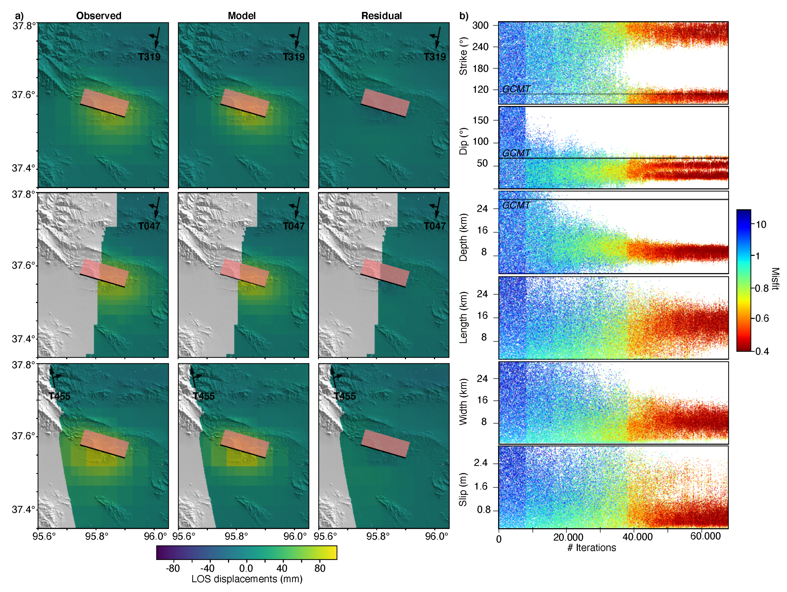
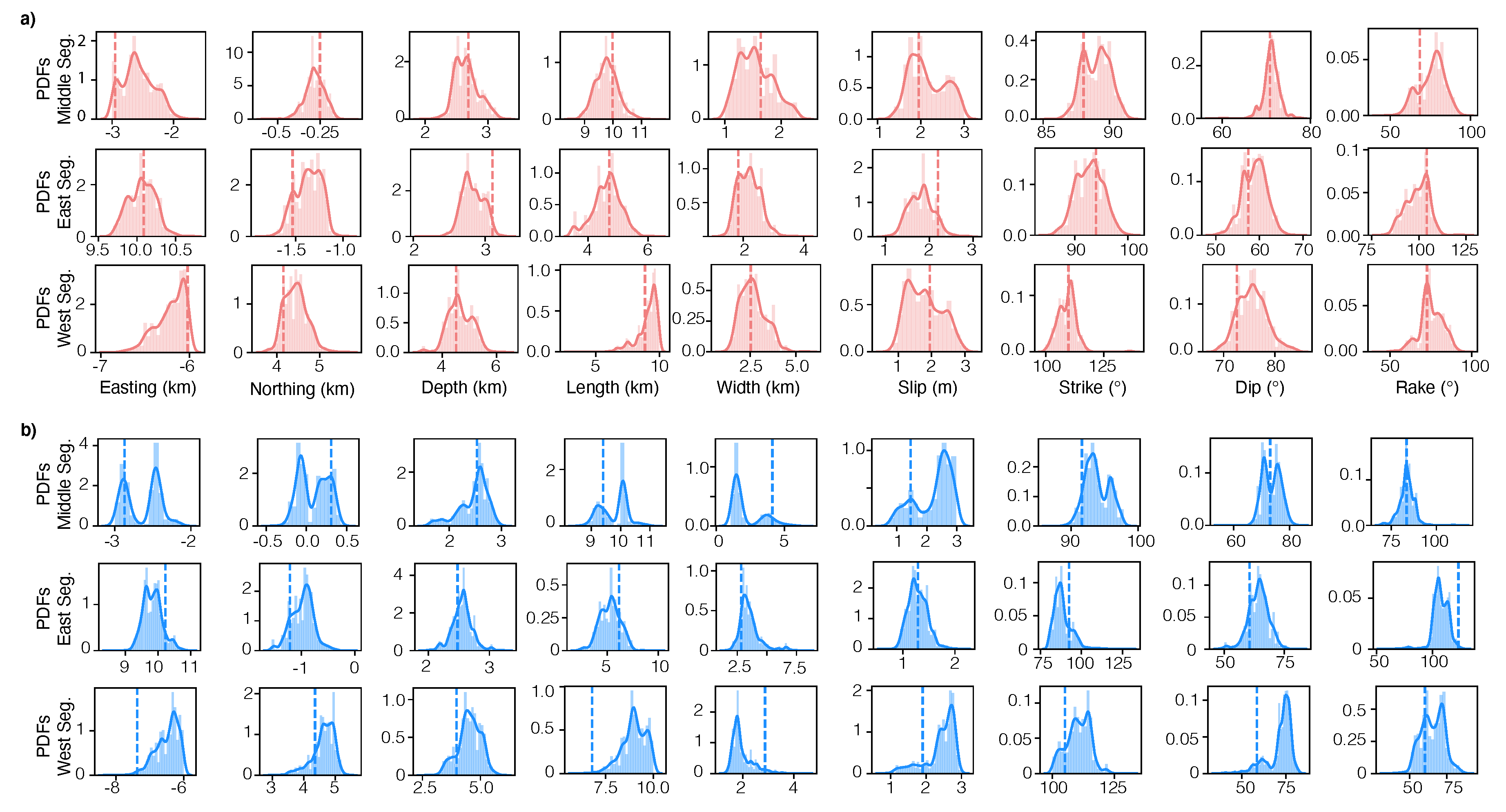
3.2. 2008 Fault Characteristics Estimations

Among north-dipping solutions for the 2008 earthquake (Figure 5 and Figure 6a), the models that best fit jointly the InSAR TS and teleseismic data feature a $16\pm 2.5$ km long and $3.6\pm 1.4$ km wide segment with a top edge center located at $11.9\pm 0.5$ km depth. The best-fitting solution converges toward a $264\pm 8^{\circ }$-striking plane dipping at a low-angle of $32\pm 2^{\circ }$ towards the north. Waveform fits for the 2008 earthquake north-dipping solution for five randomly selected stations are shown in Figure S9.

The north-dipping fault model that best explains the first four months of post-seismic deformation following the 2008 event (imaged using TS data) is a narrow segment, $18.5\pm 1.4$ km long and $0.6\pm 0.3$ km wide, with a top edge center located at $12.5\pm$ 0.8 km depth. Slip is $1.2\pm 0.4$ m for the co-seismic rupture and also of $1.2\pm 0.3$ m for the four-month post-seismic period on the narrow fault patch. While the strike of the co-seismic solution is oriented parallel to the southernmost branch of the Olongbulak Shan, the post-seismic solution has a strike of $287\pm 2^{\circ }$, perpendicular to the overall ∼N20° E regional shortening [93,94]. The dip angle is also slightly lower than the co-seismic solution, dipping at $20\pm 1.3^{\circ }$ towards the north.

In comparison, south-dipping solutions (Figure 5 and Figure 6b) converge towards a $96\pm 4^{\circ }$-striking co-seismic plane and a $102\pm 2^{\circ }$-striking post-seismic plane with high-angle dips of $60\pm 2.5^{\circ }$ and $70\pm 1.5^{\circ }$, respectively. Slip is of $1.7\pm 0.5$ m for the co-seismic rupture and of $0.05\pm 0.003$ m for the 4-month post-seismic period on the $29.7\pm 0.5$ km wide and $16.5\pm 1.4$ km long fault patch. As for the north-dipping solution, the south-dipping solution presents a very low misfit, as shown in the comparison between the geodetic data and the best-fitting model (Figure S10). While the north-dipping co- and post-seismic solutions are almost co-planar, south-dipping solutions indicate two distinct planes that are located almost ∼5 km apart.

Additionally, from the joint probabilistic inversion of the near-field stack of co-seismic interferograms and the far-field waveforms data emitted by the 2008 earthquake (Figure 7), we converge towards a $14\pm 1.8$ km long and $5.8\pm 2$ km wide rupture plane with a top edge centre located at $9.8\pm 1$ km depth. Although both north and south-dipping solutions, which are sampled during the whole optimisation (Figure 7b), show low misfit values due to the ambiguity if the displacement patterns of the buried fault plane, the best-fitting solution is a north-dipping plane striking at an angle of $286\pm {80}^{\circ }$ and dipping at an angle of $32\pm {10}^{\circ }$. There is good agreement between both geodetic and seismological observations and predictions for the three independent tracks (Figure 7a).

3.3. 2009 Fault Characteristics Estimations

For the joint probabilistic three-fault inversion of the 28 August 2009 M_w 6.3 earthquake based on InSAR and far-field teleseismic data (Figure 5), the optimisation converges towards a central segment of $10.0\pm 0.5$ km long and of $1.6\pm 0.5$ km wide with a top edge centre located at $2.7\pm 1.2$ km depth. The eastern segment is constrained with a length of $4.7\pm 0.5$ km, a width of $1.8\pm 0.5$ km, and a depth of $3.1\pm 1.5$ km, while the third western segment is of $9.0\pm 1$ km length, $2.5\pm 1$ km width, and at $4.5\pm 0.5$ km depth. All three segments have narrow widths and are, respectively, dipping with $71\pm 2^{\circ }$, $57\pm 3^{\circ }$, and $73\pm 3^{\circ }$ high-angles to the south. Slip on the fault segments amounts to $2.0\pm 0.4$ m, $2.2\pm 0.3$ m, and $1.9\pm 0.5$ m. A summary of all posterior PDFs is available in the Figure 8, while waveform fits for the 2009 earthquake north-dipping solution for five random stations are shown in Figure S9b.

Additionally, from the joint probabilistic inversion of the near-field stack of co-seismic interferograms and the far-field waveforms data emitted by the 2009 earthquake (Figure 8 and Figure S11), we converge towards a middle-segment of $9.4\pm 0.5$ km long and $4.1\pm 1.2$ km wide with a top centre edge located at $2.5\pm 0.3$ km depth. The eastern eastern segment is constrained with a length of $6.1\pm 1.0$ km, a width of $2.8\pm 0.9$ km, and a depth of $2.5\pm 0.2$ km, while the third western segment is of $6.8\pm 0.6$ km-length, $2.8\pm 0.4$ km-width, and $4.0\pm 0.5$ km-depth. The three segments all dip steeply to the south, at $73\pm 3^{\circ }$, $61\pm 4^{\circ }$, and $59\pm 7^{\circ }$, respectively. Therefore, fault geometries are very similar to the three fault segments obtained from the inversion of the co-seismic surface displacements only, and we can, therefore, reasonably conclude that post-seismic slip occurred on the same fault geometries as the coseismic rupture. Slip on the fault segments is $1.5\pm 0.6$ m, $1.3\pm 0.2$ m, and $1.9\pm 0.4$ m, respectively.

4. Discussion

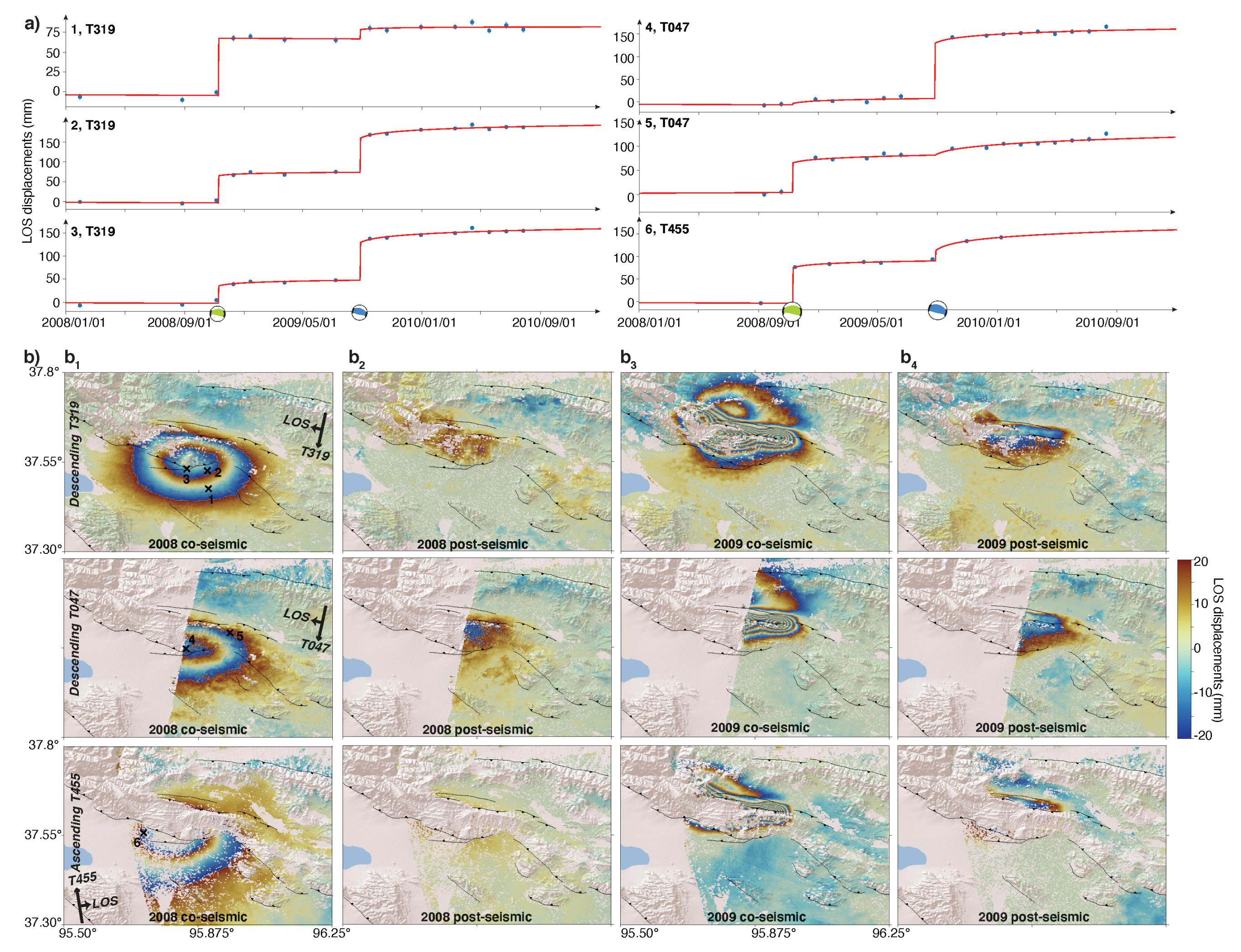
4.1. Benefits of InSAR Time Series (TS) for Fault Inference

Traditionally, an earthquake is imaged with an interferogram, which contains the phase delay between two acquisitions. However, the travel time difference between the two acquisitions does not only contain the surface displacements associated with the earthquake, but also multiple undesired signals, such as ionospheric and atmospheric delays, orbital ramps, and topographic phase errors. The interferometric phase may also include some transient post-seismic surface displacements, depending on the time span between the acquisitions prior to and after an earthquake. Therefore, in comparison to single interferograms, modeled TS maps present lower variances and covariances (Table S5). The final data variances from the TS data range from 0.2 to 3×${10}^{-6}$ m², while the correlation lengths are about 0.5–2 km.

The stack of co-seismic interferograms also helps to improve the unwrapping coverage and the signal-to-noise ratio. Stacking is a simple way of removing turbulent atmospheric phase patterns that are random in time and space, and improves the spatial coverage, as interferograms used for the stack have varying unwrapping coverage, depending on their temporal and geometrical baselines and their respective noises. Conversely, TS data only have information for pixels where the TS analysis and the time decomposition is possible, ie. when there is enough unwrapped interferogram for a given pixel for the inversion to be reliable. However, and contrary to a TS approach, a stack may also constructively add tropospheric signal if it is of the same sign in all stacked interferograms and, therefore, may also contain more correlated noise than differential interferograms, as illustrated by the higher correlation length values of the stacked data in Table S5. In addition, by using long-temporal baseline interferograms that cover the post-seismic period within the stack, the stacking operation also increases the amount of post-seismic deformation within the data. This effect is illustrated in the 2008 fault inference constrained with stacked interferograms as posterior solutions are spatially located between co-seismic and post-seismic solutions inferred with the TS data (Figure 7a).

We perform another north-dipping 2008 co-seismic fault inference jointly constrained with the DInSAR interferograms shown in Figure 3 and with teleseismic data in order to further evaluate the benefits of the TS approach. We then compare the posterior PDFs with those derived from the joint inversion of co-seismic TS maps and teleseismic data (Figure 9). The analysis shows that, as for the solution constrained with the stack of co-seismic interferograms (Figure 7), the fault parameters inference constrained with DInSAR are biased towards a solution that averages the co-seismic and the post-seismic solutions derived from TS data (Figure 6). The solution is pushed further north, where post-seismic slip occurred, at $10\pm 0.2$ km of the gCMT solution, and towards a $18.2\pm 2.2$ km long and narrow $1.7\pm 0.4$ km wide rupture plane with a top located at $12.1\pm 0.5$ km depth. Posterior PDFs of the depth indicate higher values for the DInSAR optimisations than the TS optimisations, which is also in agreement with the fact that post-seismic slip occurred at a greater depth than the co-seismic slip (Figure 6). The best-fitting values for slip, strike, and rake are $2.0\pm 0.4$ m, $284\pm {14}^{\circ }$, and $87\pm {15}^{\circ }$, and their PDFs are wider than those that were obtained from the inversion of TS and teleseismic data. Slip for DInSAR is also expected to be higher due to the presence of early afterslip in the data. The DInSAR best-fitting $22\pm 4^{\circ }$ northward dip angle is ∼10° lower than the dip angle reported in the gCMT catalog and the one of the northward-dip constrained by TS solutions, but again closer to the dip solution obtained from the post-seismic fault (Figure 6). Posterior PDFs of the easting, depth, slip, strike, dip, and rake parameters have higher standard deviations when constrained from DInSAR than the TS maps, but, inversely, posterior PDFs for the northing and width fault parameters are narrower with DInSAR. This comparison shows that the inclusion of afterslip in the co-seismic modelling may introduce some large biases in the results towards the post-seismic solution. Those biases are proportional to the magnitude of the aseismic slip and the period between the two acquisitions of the co-seismic interferogram. Additionally, higher posterior uncertainties in the fault characteristics estimation are expected for the DInSAR optimisation in comparison to TS due to the higher noise in the co-seismic interferograms. However, wider PDFs for DInSAR is not, in this case, clearly highlighted for all parameters, which may be due to efficient empirical corrections performed on the DInSAR interferograms.

A pixel-by-pixel decomposition of the cumulative InSAR displacement TS has the limitation of providing a solution that may not have a spatial physical meaning and with reliability that depends on the number of acquisition dates and/or on the residual noise in the TS data. A multi-pixel TS decomposition approach [95] may tackle part of these limitations by accounting for the spatially correlated noise in the surface displacement data. However, the spatial consistency that was obtained in the decomposition (Figure 2) validates the pixel-by-pixel method and the reliability of the results. In addition, the simplicity of the inverse problem (contrary to a multi-pixel approach that demands the inversion of a large matrix function of the number of InSAR points) allows us to perform optimisation with some additional constraints, such as imposing post-seismic surface displacements of the same sign than co-seismic surface displacements. An alternative approach would be a decomposition of the InSAR time-series data by joint and direct inversion of slip on the co-seismic and post-seismic fault planes. Such an approach would impose a physical meaning of the decomposition contrary to a pixel-by-pixel or multi-pixel decomposition in time. However, it also requires a fixed fault geometry e.g., [30,43,48,50] as the joint optimisation of both fault source parameters and temporal basis functions for each InSAR point is computationally expensive and such a modelling tool is currently not available to our knowledge.

4.2. Back-Projection Imaging for Moderate-Size Earthquakes

The derived 2008 earthquake’s beam-power time function (Figure 4a) is very similar to the source time function from the SCARDEC database [96] (http://scardec.projects.sismo.ipgp.fr/). Of particular note, the method retrieves information about the source of the 2009 earthquake even if some waveforms might be contaminated by the 2009 Banda Sea Earthquake. Therefore, the method shows its efficiency in comparison to other approaches to suppress unwanted signals arriving from other azimuths through destructive inferences [67]. It is robust against signals from outside the defined source grid due to the stacking procedure.

The back-projection tool has also located the coherent emissions of both earthquakes with a remarkable agreement with geodetic data. It also shows, with the 2009 earthquake, promise as a method to infer the level of segmentation of a rupture without formal kinematic modelling, even for moderately sized earthquakes.

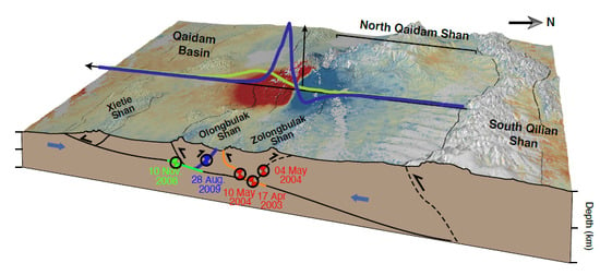
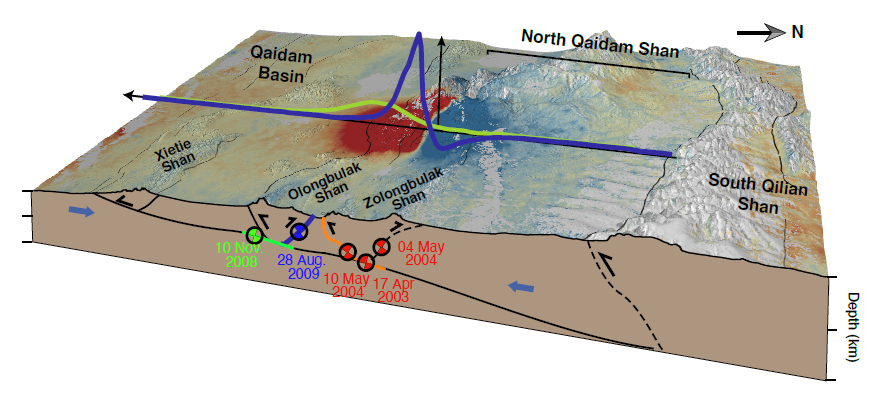
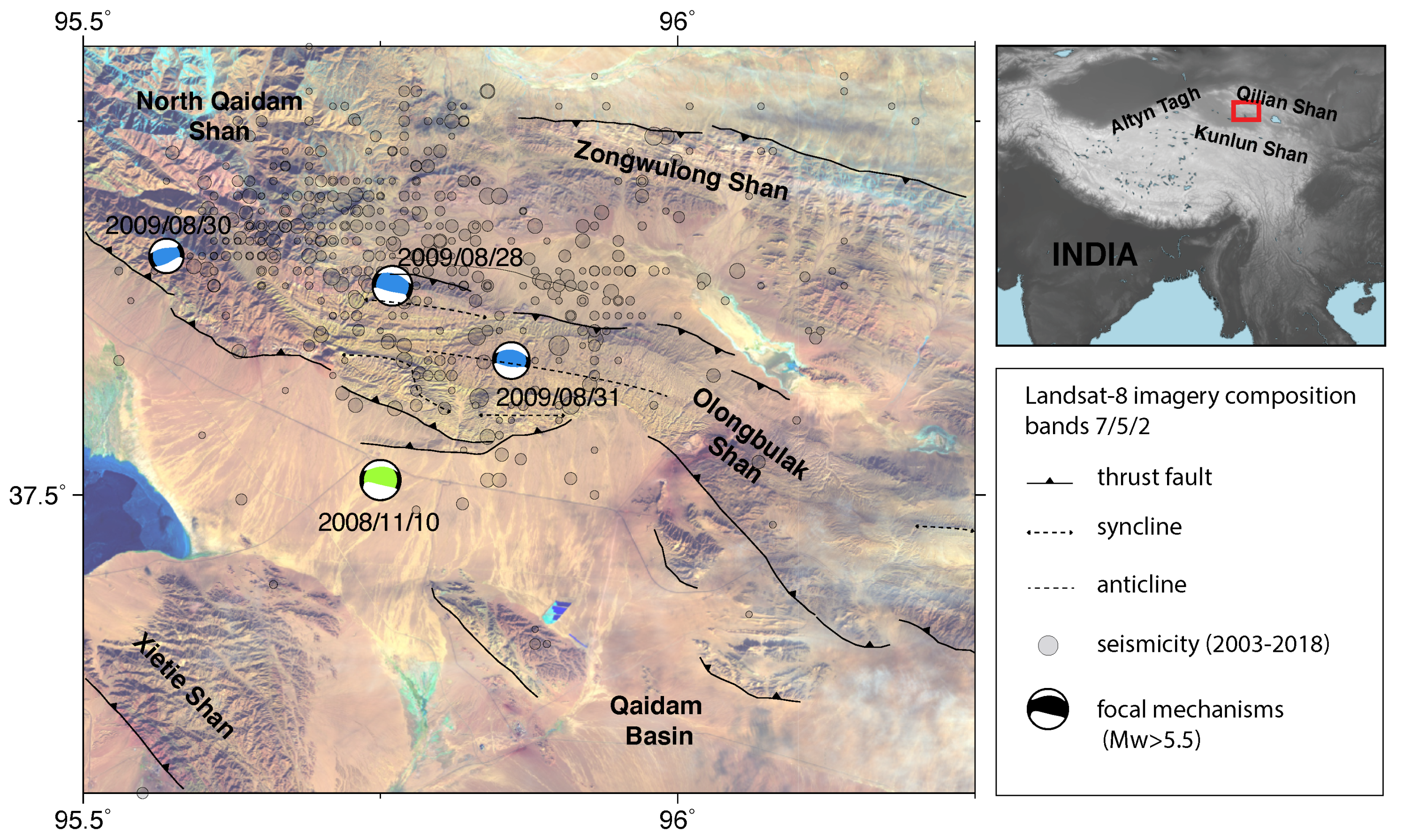
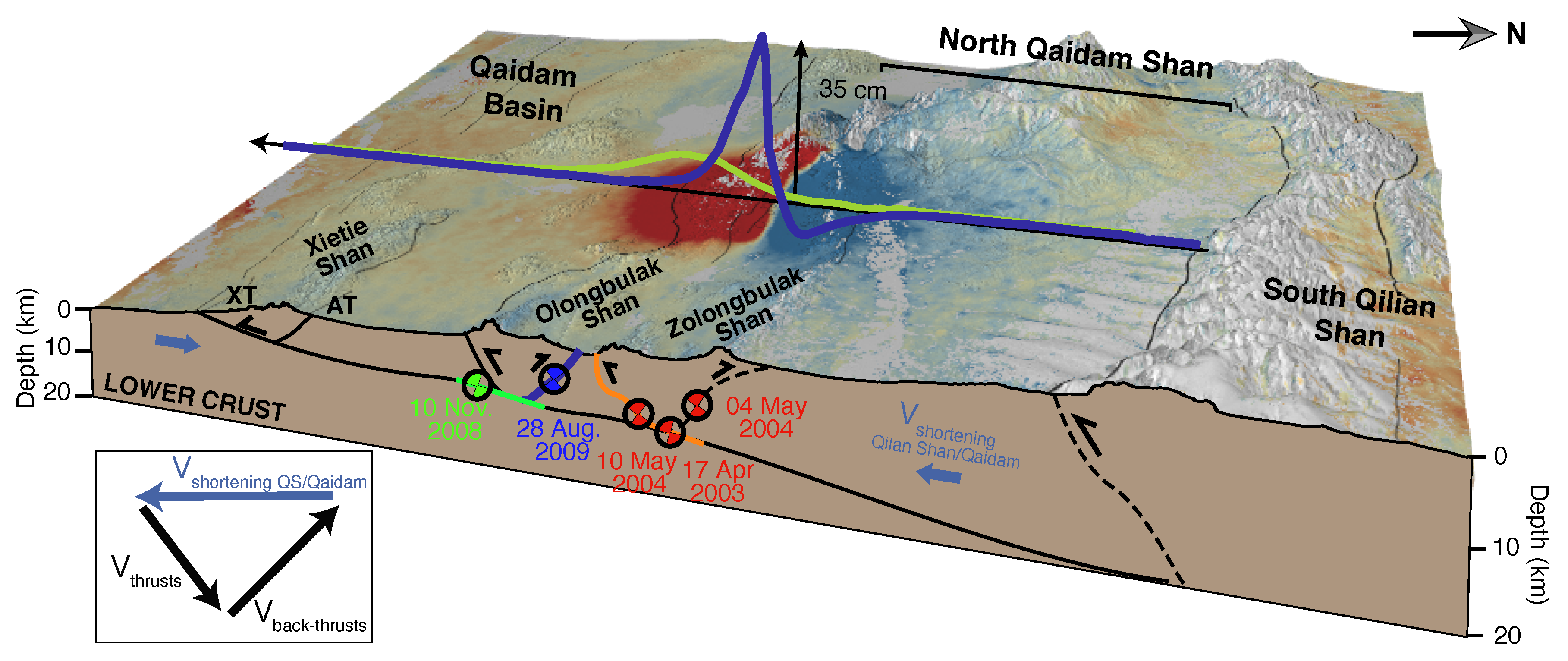
4.3. The 2008–2009 Qaidam Earthquake Sequence

By reconciling co- and post-seismic geodetic observations, back-projection imaging, kinematic fault inferences, and previous structural interpretations, we develop a model for the fault geometry of the Qaidam thrust system shown in Figure 10, with overall fault and fold geometry typical of foreland fold-and-thrust belts

Daout et al., 2019 [45] modeled, from Envisat measurements across the Zolonbulak Shan, the short-term after-slip following the 17 April 2003 Delingha earthquake with a shallow segmented ramp-flat-ramp north-dipping structure that steepens as it approaches the surface under the Delingha anticline, and inferred a low-angle north-dipping fault for the 2003 earthquake (orange line in Figure 10). The north-dipping gCMT solution of the 2003 earthquake is very similar to the 2008 gCMT solution with a ∼30° dip angle rupture plane at about 16 km depth (Table S1, red focal mechanism in Figure 10). In addition, the two ∼18 km and ∼21 km deep April 2004 right-lateral ∼M_w 5.3 earthquakes and the ∼12 km deep October 2004 thrust ∼M_w 5.5 earthquake (according to gCMT, Table S1) may belong to the same flower structure that ruptured in 2003 (Figure 10). Static stress transfer within this flower structure may have triggered the 2004 sequence of earthquakes one year after the 2003 earthquake.

This study show that kinematic inversion alone cannot rigorously resolve the ambiguity between the north-dipping and south-dipping geometries due to the low misfits of both solutions. Biases may also arise from assumptions on the 1D crustal structure or the absence of topography in the model, although bootstrapping technique can efficiently estimate model parameter uncertainties by propagating data errors and by assessing modelling errors. In addition, the stations have individual time shifts to compensate for crustal structures, such as each station can shift its waveforms up to 4 s with respect to the earthquakes’ onset time to achieve maximum fit. This compensates for unmodeled three-dimensional (3D)-path effects.

Here, we infer a shallow north-dipping low-angle structure that is responsible for the 2008 earthquake (green line in Figure 10), mainly constrained from the coplanarity between the co- and post-seismic north-dipping solutions (Figure 5). The depth of the rupture (∼12 km deep) is in agreement with the width of the Olongbukak range (∼10–15 km), as north-dipping and south-dipping faults bounding the Olongbulak range are expected to merge as those depths (Figure 5). The presence in the morphology of a major north-dipping structure in the southern front of the Olongbulak range also challenges a hypothetic south-dipping and high-angle 2008 rupture plane, coplanar to the 2009 rupture (Figures S1b and S12). Such coplanar fault geometries would not create a differential vertical movement between the deeper part of the south-dipping fault (where the 2008 earthquake occurred) and the shallow part of the fault, within the Olongbulak Shan (where the 2009 earthquake occurred) [19] (Figure S12b). The absence of differential vertical movements would, therefore, require no triple junction and shallow high-angle north-dipping plane, while this structure is identified in the southern front of the Olongbulak Shan. As a triple junction is not stable over long time scale and, as the current morphology involves multiples deformation stages, it is difficult to conclude from this observation. However, the main north-dipping vergence of the NQT and the current activity of its southernmost branches, as within the Olongbulak pop-up, support our view of a low-angle north-dipping plane, responsible for the 2003 and 2008 earthquakes, branching at the roots of the shallow high-angle thrusts of the NQ ranges and of the Qaidam basin.

Our results also indicate that the 2008 earthquake did not break the southern and north-dipping high-angle branch of the Olongbulak pop-up structure. Post-seismic slip is constrained down-dip of the co-seismic rupture on a very narrow plane with slip of the same order of magnitude than the co-seismic slip. Surface displacements might not be very sensitive to the amount of down-dip afterslip, and the amount of slip might, therefore, be over-estimated for the north-dipping solution. In this regard, we performed several tests forcing a higher fault width or lower fault slip. We observed that with such prior values, posterior PDFs tend to be asymmetric towards the boundary values, indicating that the data require such high slip and narrow fault width. The modelling, therefore, shows that the observed short-term post-seismic displacements cannot be explained by fault movement on the north-dipping shallow and high-angle branch of the Olongbulak pop-up structure, thus leaving an open question on the seismic potential of this branch of the Olongbulak range.

The 2009 rupture is the result of the vertical partitioning of the shortening along the high-angle and shallow south-dipping back-thrust of the Olongbulak Shan (blue line in Figure 10). The rupture started at ∼9 km depth along the middle segment and then propagated bilaterally along two shallower and higher-angle segments (Figure 4 and Figure 5) that displace basin-deformed sediments of the Olongbulak range above the Paleozoic bedrock of the Zonlongbulak range [47,57,97]. Afterslip likely occurred on a similar fault patch surrounding the coseismic slip, in agreement with similar post-seismic and co-seismic surface displacement patterns measured with InSAR (Figure 2 and Figure 3), the optimisation of the stack of long- and short-temporal baselines interferograms (Figure S11), and previous studies [48,49,50]. The observed rupture complexity in both geodetic displacements and back-projected seismic emissions likely reflect the along strike and along depth lithological segmentation of the Olongbulak fault system.

The 2008–2009 Qaidam earthquake sequence illuminates a short-timescale and spatially confined example of regional tectonic and geodynamic processes at play. However, the inferred flower structure, in which high-angle thrusts and back-thrusts root into a low-angle décollement, may be typical of structures and deformation styles in the South Qilian Shan at greater scale. The low-angle north-dipping structure may connect to the roots of the Olongbulak pop-up structure, the Zongbulak Shan, and the Xietie Shan thrusts and may transfer the shortening rate from the north, along the Qilian Shan, to south, in Qaidam Basin, along the high-angle folds and thrust belts (Figure 10, inset, Figure S1a). It supports regional tectonic models that involve a regional décollement that connects to the Qilian Shan suture or pre-existing Cenozoic lithospheric weaknesses further north [52,54,57,59] and the southward expansion of the South Qilian Shan [60,97].

5. Conclusions

In this study, we explore the benefits of an InSAR TS approach for earthquake fault inference and demonstrate the improved signal-to-noise ratio of such data sets in comparison to DInSAR, and the additional constraints offered by the post-seismic surface displacements that were extracted from the InSAR TS data. The 2008–2009 Qaidam earthquake sequence exemplifies typical earthquakes in remote areas, where field work is difficult and structural seismic profile or geological models are rarely available or poorly constrained, yet satellite-based geodetic and teleseismic data are easily available. We use the open source Grond toolbox [81], the Pyrocko framework [98] and the Kite toolbox [40] for pre-processing and analysing surface displacements to infer the earthquake fault parameters from both geodetic and teleseismic data. Pyrocko provides a uniform framework for both near-field and far-field data and Green’s function databases to speed up forward calculations. Our analysis reveals that the optimisation scheme successfully explores bimodal north-dipping and south-dipping solutions for the deep 2008 earthquake, which was further validated based on the co-planarity between the inferred co-seismic and post-seismic fault planes. It also shows that the tool allows the exploration of the rupture segmentations with three independent faults, where no fault geometrical parameters are fixed a priori. Besides, the back-projection tool, also based on the Pyrocko framework, has located the coherent emissions of both earthquakes with a remarkable agreement with geodetic data. It also constrains the segmentation of 2009 ruptures in accordance with the InSAR-based fault models and, therefore, shows promise as a useful tool, even for moderate earthquakes.

References

1. Duputel, Z.; Agram, P.S.; Simons, M.; Minson, S.E.; Beck, J.L. Accounting for prediction uncertainty when inferring subsurface fault slip. Geophys. J. Int. 2014, 197, 464–482. [Google Scholar] [CrossRef] [Green Version]
2. Ragon, T.; Sladen, A.; Simons, M. Accounting for uncertain fault geometry in earthquake source inversions—I: Theory and simplified application. Geophys. J. Int. 2018, 214, 1174–1190. [Google Scholar] [CrossRef]
3. Langer, L.; Ragon, T.; Sladen, A.; Tromp, J. Impact of topography on earthquake static slip inversions. Tectonophysics 2020, 228566. [Google Scholar] [CrossRef] [Green Version]
4. Steinberg, A.; Sudhaus, H.; Heimann, S.; Krüger, F. Sensitivity of InSAR and teleseismic observations to earthquake rupture segmentation. Geophys. J. Int. 2020, 223, 875–907. [Google Scholar] [CrossRef]
5. Mai, P.M.; Schorlemmer, D.; Page, M.; Ampuero, J.P.; Asano, K.; Causse, M.; Custodio, S.; Fan, W.; Festa, G.; Galis, M.; et al. The earthquake-source inversion validation (SIV) project. Seismol. Res. Lett. 2016, 87, 690–708. [Google Scholar] [CrossRef]
6. Bletery, Q.; Sladen, A.; Delouis, B.; Vallée, M.; Nocquet, J.M.; Rolland, L.; Jiang, J. A detailed source model for the Mw9. 0 Tohoku-Oki earthquake reconciling geodesy, seismology, and tsunami records. J. Geophys. Res. Solid Earth 2014, 119, 7636–7653. [Google Scholar] [CrossRef] [Green Version]
7. Marchandon, M.; Vergnolle, M.; Sudhaus, H.; Cavalié, O. Fault Geometry and Slip Distribution at Depth of the 1997 Mw 7.2 Zirkuh Earthquake: Contribution of Near-Field Displacement Data. J. Geophys. Res. Solid Earth 2018, 123, 1904–1924. [Google Scholar] [CrossRef]
8. Akoğlu, A.M.; Jónsson, S.; Wang, T.; Çakır, Z.; Dogan, U.; Ergintav, S.; Osmanoğlu, B.; Feng, G.; Zabcı, C.; Özdemir, A.; et al. Evidence for tear faulting from new constraints of the 23 October 2011 Mw 7.1 van, Turkey, earthquake based on InSAR, GPS, coastal uplift, and field observationsevidence for tear faulting from new constraints of the 2011 van, Turkey, earthquake. Bull. Seismol. Soc. Am. 2018, 108, 1929–1946. [Google Scholar] [CrossRef]
9. Gombert, B.; Duputel, Z.; Jolivet, R.; Doubre, C.; Rivera, L.; Simons, M. Revisiting the 1992 Landers earthquake: A Bayesian exploration of co-seismic slip and off-fault damage. Geophys. J. Int. 2018, 212, 839–852. [Google Scholar] [CrossRef] [Green Version]
10. Weston, J.; Ferreira, A.; Funning, G. Joint earthquake source inversions using seismo-geodesy and 3-D earth models. Geophys. J. Int. 2014, 198, 671–696. [Google Scholar] [CrossRef] [Green Version]
11. Huang, M.H.; Tung, H.; Fielding, E.J.; Huang, H.H.; Liang, C.; Huang, C.; Hu, J.C. Multiple fault slip triggered above the 2016 Mw 6.4 MeiNong earthquake in Taiwan. Geophys. Res. Lett. 2016, 43, 7459–7467. [Google Scholar] [CrossRef] [Green Version]
12. Frietsch, M.; Ferreira, A.; Funning, G.; Weston, J. Multiple fault modelling combining seismic and geodetic data: The importance of simultaneous subevent inversions. Geophys. J. Int. 2019, 218, 958–976. [Google Scholar] [CrossRef] [Green Version]
13. Vasyura-Bathke, H.; Dettmer, J.; Steinberg, A.; Heimann, S.; Isken, M.P.; Zielke, O.; Mai, P.M.; Sudhaus, H.; Jónsson, S. The Bayesian Earthquake Analysis Tool. Seismol. Res. Lett. 2020, 91, 1003–1018. [Google Scholar] [CrossRef]
14. Lohman, R.B.; Simons, M. Some thoughts on the use of InSAR data to constrain models of surface deformation: Noise structure and data downsampling. Geochem. Geophys. Geosyst. 2005, 6. [Google Scholar] [CrossRef]
15. Sudhaus, H.; Sigurjón, J. Improved source modelling through combined use of InSAR and GPS under consideration of correlated data errors: Application to the June 2000 Kleifarvatn earthquake, Iceland. Geophys. J. Int. 2009, 176, 389–404. [Google Scholar] [CrossRef] [Green Version]
16. Cesca, S.; Letort, J.; Razafindrakoto, H.N.; Heimann, S.; Rivalta, E.; Isken, M.P.; Nikkhoo, M.; Passarelli, L.; Petersen, G.M.; Cotton, F.; et al. Drainage of a deep magma reservoir near Mayotte inferred from seismicity and deformation. Nat. Geosci. 2020, 13, 87–93. [Google Scholar] [CrossRef]
17. Minson, S.; Simons, M.; Beck, J. Bayesian inversion for finite fault earthquake source models I. Theory and algorithm. Geophys. J. Int. 2013, 194, 1701–1726. [Google Scholar] [CrossRef] [Green Version]
18. Minson, S.; Simons, M.; Beck, J.; Ortega, F.; Jiang, J.; Owen, S.; Moore, A.; Inbal, A.; Sladen, A. Bayesian inversion for finite fault earthquake source models–II: The 2011 great Tohoku-oki, Japan earthquake. Geophys. J. Int. 2014, 198, 922–940. [Google Scholar] [CrossRef]
19. Daout, S.; Barbot, S.; Peltzer, G.; Doin, M.P.; Liu, Z.; Jolivet, R. Constraining the Kinematics of Metropolitan Los Angeles Faults with a Slip-Partitioning Model. Geophys. Res. Lett. 2016, 43, 11–192. [Google Scholar] [CrossRef]
20. Hong, S.; Zhou, X.; Zhang, K.; Meng, G.; Dong, Y.; Su, X.; Zhang, L.; Li, S.; Ding, K. Source model and stress disturbance of the 2017 Jiuzhaigou Mw 6.5 earthquake constrained by InSAR and GPS measurements. Remote Sens. 2018, 10, 1400. [Google Scholar] [CrossRef] [Green Version]
21. Wright, T.J.; Parsons, B.E.; Lu, Z. Toward mapping surface deformation in three dimensions using InSAR. Geophys. Res. Lett. 2004, 31. [Google Scholar] [CrossRef] [Green Version]
22. Lasserre, C.; Peltzer, G.; Crampé, F.; Klinger, Y.; Van der Woerd, J.; Tapponnier, P. Coseismic deformation of the 2001 Mw = 7.8 Kokoxili earthquake in Tibet, measured by synthetic aperture radar interferometry. J. Geophys. Res. 2005, 110. [Google Scholar] [CrossRef] [Green Version]
23. Sudhaus, H.; Jónsson, S. Source model for the 1997 Zirkuh earthquake (MW = 7.2) in Iran derived from JERS and ERS InSAR observations. Geophys. J. Int. 2011, 185, 676–692. [Google Scholar] [CrossRef] [Green Version]
24. Elliott, J.; Jolivet, R.; González, P.; Avouac, J.P.; Hollingsworth, J.; Searle, M.; Stevens, V. Himalayan megathrust geometry and relation to topography revealed by the Gorkha earthquake. Nat. Geosci. 2016, 9, 174–180. [Google Scholar] [CrossRef] [Green Version]
25. Mackenzie, D.; Elliott, J.; Altunel, E.; Walker, R.; Kurban, Y.; Schwenninger, J.L.; Parsons, B. Seismotectonics and rupture process of the Mw 7.1 2011 Van reverse-faulting earthquake, eastern Turkey, and implications for hazard in regions of distributed shortening. Geophys. J. Int. 2016, 206, 501–524. [Google Scholar] [CrossRef] [Green Version]
26. Ganas, A.; Kourkouli, P.; Briole, P.; Moshou, A.; Elias, P.; Parcharidis, I. Coseismic displacements from moderate-size earthquakes mapped by Sentinel-1 differential interferometry: The case of February 2017 Gulpinar earthquake sequence (Biga Peninsula, Turkey). Remote Sens. 2018, 10, 1089. [Google Scholar] [CrossRef] [Green Version]
27. Hanssen, R.F. Radar Interferometry: Data Interpretation and Error Analysis; Springer Science & Business Media: Berlin/Heidelberg, Germany, 2001; Volume 2. [Google Scholar]
28. Doin, M.P.; Lasserre, C.; Peltzer, G.; Cavalié, O.; Doubre, C. Corrections of stratified tropospheric delays in SAR interferometriy: Validation with global atmospheric models. J. Appl. Geophys. 2009, 69, 35–50. [Google Scholar] [CrossRef]
29. Gomba, G.; Parizzi, A.; De Zan, F.; Eineder, M.; Bamler, R. Toward operational compensation of ionospheric effects in SAR interferograms: The split-spectrum method. IEEE Trans. Geosci. Remote Sens. 2015, 54, 1446–1461. [Google Scholar] [CrossRef] [Green Version]
30. Floyd, M.A.; Walters, R.J.; Elliott, J.R.; Funning, G.J.; Svarc, J.L.; Murray, J.R.; Hooper, A.J.; Larsen, Y.; Marinkovic, P.; Bürgmann, R.; et al. Spatial variations in fault friction related to lithology from rupture and afterslip of the 2014 South Napa, California, earthquake. Geophys. Res. Lett. 2016, 43, 6808–6816. [Google Scholar] [CrossRef] [Green Version]
31. Ragon, T.; Sladen, A.; Bletery, Q.; Vergnolle, M.; Cavalié, O.; Avallone, A.; Balestra, J.; Delouis, B. Joint Inversion of Coseismic and Early Postseismic Slip to Optimize the Information Content in Geodetic Data: Application to the 2009 M w 6.3 L’Aquila Earthquake, Central Italy. J. Geophys. Res. Solid Earth 2019, 124, 10522–10543. [Google Scholar] [CrossRef] [Green Version]
32. Massonnet, D.; Rossi, M.; Carmona, C.; Adragna, F.; Peltzer, G.; Feigl, K.; Rabaute, T. The displacement field of the Landers earthquake mapped by radar interferometry. Nature 1993, 364, 138–142. [Google Scholar] [CrossRef]
33. Berardino, P.; Fornaro, G.; Lanari, R.; Sansosti, E. A new algorithm for surface deformation monitoring based on small baseline differential SAR interferograms. IEEE Trans. Geosci. Remote Sens. 2002, 40, 2375–2383. [Google Scholar] [CrossRef] [Green Version]
34. Hooper, A. A multi-temporal InSAR method incorporating both persistent scatterer and small baseline approaches. Geophys. Res. Lett. 2008, 35. [Google Scholar] [CrossRef] [Green Version]
35. Doin, M.P.; Twardzik, C.; Ducret, G.; Lasserre, C.; Guillaso, S.; Jianbao, S. InSAR measurement of the deformation around Siling Co Lake: Inferences on the lower crust viscosity in central Tibet. J. Geophys. Res. Solid Earth 2015, 120, 5290–5310. [Google Scholar] [CrossRef]
36. Jolivet, R.; Grandin, R.; Lasserre, C.; Doin, M.P.; Peltzer, G. Systematic InSAR tropospheric phase delay corrections from global meteorological reanalysis data. Geophys. Res. Lett. 2011, 38. [Google Scholar] [CrossRef] [Green Version]
37. Daout, S.; Dini, B.; Haeberli, W.; Doin, M.P.; Parsons, B. Ice loss in the Northeastern Tibetan Plateau permafrost as seen by 16 yr of ESA SAR missions. Earth Planet. Sci. Lett. 2020, 545, 116404. [Google Scholar] [CrossRef]
38. Cavalié, O.; Doin, M.P.; Lasserre, C.; Briole, P. Ground motion measurement in the Lake Mead area, Nevada, by differential synthetic aperture radar interferometry time series analysis: Probing the lithosphere rheological structure. J. Geophys. Res. 2007, 112. [Google Scholar] [CrossRef] [Green Version]
39. Lin, Y.n.N.; Simons, M.; Hetland, E.A.; Muse, P.; DiCaprio, C. A multiscale approach to estimating topographically correlated propagation delays in radar interferograms. Geochem. Geophys. Geosyst. 2010, 11. [Google Scholar] [CrossRef]
40. Isken, M.; Sudhaus, H.; Heimann, S.; Steinberg, A.; Daout, S.; Vasyura-Bathke, H. Kite—Software for Rapid Earthquake Source Optimisation from InSAR Surface Displacement. GFZ Data Serv. 2017. [Google Scholar] [CrossRef]
41. Yu, C.; Li, Z.; Penna, N.T.; Crippa, P. Generic atmospheric correction model for Interferometric Synthetic Aperture Radar observations. J. Geophys. Res. Solid Earth 2018, 123, 9202–9222. [Google Scholar] [CrossRef]
42. Dini, B.; Daout, S.; Manconi, A.; Loew, S. Classification of slope processes based on multitemporal DInSAR analyses in the Himalaya of NW Bhutan. Remote Sens. Environ. 2019, 233, 111408. [Google Scholar] [CrossRef]
43. Wimpenny, S.; Copley, A.; Ingleby, T. Fault mechanics and post-seismic deformation at Bam, SE Iran. Geophys. J. Int. 2017, 209, 1018–1035. [Google Scholar] [CrossRef] [Green Version]
44. Barnhart, W.D.; Brengman, C.M.; Li, S.; Peterson, K.E. Ramp-flat basement structures of the Zagros Mountains inferred from co-seismic slip and afterslip of the 2017 Mw 7.3 Darbandikhan, Iran/Iraq earthquake. Earth Planet. Sci. Lett. 2018, 496, 96–107. [Google Scholar] [CrossRef]
45. Daout, S.; Sudhaus, H.; Kausch, T.; Steinberg, A.; Dini, B. Interseismic and postseismic shallow creep of the North Qaidam Thrust faults detected with a multitemporal InSAR analysis. J. Geophys. Res. Solid Earth 2019, 124, 7259–7279. [Google Scholar] [CrossRef]
46. Elliott, J.; Parsons, B.; Jackson, J.; Shan, X.; Sloan, R.; Walker, R. Depth segmentation of the seismogenic continental crust: The 2008 and 2009 Qaidam earthquakes. Geophys. Res. Lett. 2011, 38. [Google Scholar] [CrossRef]
47. Guihua, C.; Xiwei, X.; Ailan, Z.; Xiaoqing, Z.; Renmao, Y.; Klinger, Y.; Nocquet, J.M. Seismotectonics of the 2008 and 2009 Qaidam earthquakes and its implication for regional tectonics. Acta Geol. Sin. Engl. Ed. 2013, 87, 618–628. [Google Scholar] [CrossRef]
48. Feng, W. Modelling Co-and Post-Seismic Displacements Revealed by InSAR, and Their Implications for Fault Behaviour. Ph.D. Thesis, University of Glasgow, Glasgow, UK, 2015. [Google Scholar]
49. Liu, Y.; Xu, C.; Wen, Y.; Li, Z. Post-seismic deformation from the 2009 Mw 6.3 Dachaidan earthquake in the northern Qaidam Basin detected by small baseline subset InSAR technique. Sensors 2016, 16, 206. [Google Scholar] [CrossRef] [Green Version]
50. Liu, Y.; Xu, C.; Li, Z.; Wen, Y.; Chen, J.; Li, Z. Time-dependent afterslip of the 2009 mw 6.3 dachaidan earthquake (China) and viscosity beneath the qaidam basin inferred from postseismic deformation observations. Remote Sens. 2016, 8, 649. [Google Scholar] [CrossRef] [Green Version]
51. Daout, S.; Doin, M.P.; Peltzer, G.; Socquet, A.; Lasserre, C. Large scale InSAR monitoring of permafrost freeze-thaw cycles on the Tibetan Plateau. Geophys. Res. Lett. 2017. [Google Scholar] [CrossRef]
52. Burchfiel, B.; Quidong, D.; Molnar, P.; Royden, L.; Yipeng, W.; Peizhen, Z.; Weiqi, Z. Intracrustal detachment within zones of continental deformation. Geology 1989, 17, 748–752. [Google Scholar] [CrossRef]
53. Métivier, F.; Gaudemer, Y.; Tapponnier, P.; Meyer, B. Northeastward growth of the Tibet Plateau deduced from balanced reconstruction of two depositional areas: The Qaidam and Hexi Corridor Basins, China. Tectonics 1998, 17, 823–842. [Google Scholar] [CrossRef] [Green Version]
54. Meyer, B.; Tapponnier, P.; Bourjot, L.; Metivier, F.; Gaudemer, Y.; Peltzer, G.; Shunmin, G.; Zhitai, C. Crustal thickening in Gausu-Qinghai, lithospheric mantle subduction, and oblique, strike-slip controlled growth of the Tibet Plateau. Geophy. J. Int. 1998, 135, 1–47. [Google Scholar] [CrossRef]
55. Tapponnier, P.; Zhiqin, X.; Roger, F.; Meyer, B.; Arnaud, N.; Wittlinger, G.; Jingsui, Y. Oblique Stepwise Rise and Growth of the Tibet Plateau. Science 2001, 294, 1671–1677. [Google Scholar] [CrossRef] [PubMed]
56. Dupont-Nivet, G.; Horton, B.; Butler, R.F.; Wang, J.; Zhou, J.; Waanders, G. Paleogene clockwise tectonic rotation of the Xining-Lanzhou region, northeastern Tibetan Plateau. J. Geophys. Res. Solid Earth 2004, 109. [Google Scholar] [CrossRef] [Green Version]
57. Yin, A.; Dang, Y.Q.; Wang, L.C.; Jiang, W.M.; Zhou, S.P.; Chen, X.H.; Gehrels, G.E.; McRivette, M.W. Cenozoic tectonic evolution of Qaidam Basin and its surrounding regions (Part 1): The southern Qilian Shan-Nan Shan thrust belt and northern Qaidam Basin. Geol. Soc. Am. Bull. 2008, 120, 813–846. [Google Scholar] [CrossRef]
58. Bush, M.A.; Saylor, J.E.; Horton, B.K.; Nie, J. Growth of the Qaidam Basin during Cenozoic exhumation in the northern Tibetan Plateau: Inferences from depositional patterns and multiproxy detrital provenance signatures. Lithosphere 2016, 8, 58–82. [Google Scholar] [CrossRef]
59. Yin, A.; Harrison, T.M. Geologic evolution of the Himalayan-Tibetan orogen. Annu. Rev. Earth Planet. Sci. 2000, 28, 211–280. [Google Scholar] [CrossRef] [Green Version]
60. Yin, A.; Dang, Y.Q.; Zhang, M.; Chen, X.H.; McRivette, M.W. Cenozoic tectonic evolution of the Qaidam Basin and its surrounding regions (Part 3): Structural geology, sedimentation, and regional tectonic reconstruction. Geol. Soc. Am. Bull. 2008, 120, 847–876. [Google Scholar] [CrossRef] [Green Version]
61. England, P.C.; Houseman, G. The mechanics of the Tibetan Plateau. Phil. Trans. R. Soc. Lond. A 1988, 326, 301–320. [Google Scholar]
62. Royden, L.H.; Burchfiel, B.C.; King, R.W.; Wang, E.; Chen, Z.; Shen, F.; Liu, Y. Surface deformation and lower crustal flow in eastern Tibet. Science 1997, 276, 788–790. [Google Scholar] [CrossRef]
63. Clark, M.K.; Royden, L.H. Topographic ooze: Building the eastern margin of Tibet by lower crustal flow. Geology 2000, 28, 703–706. [Google Scholar] [CrossRef]
64. Ekström, G.; Nettles, M.; Dziewoński, A. The global CMT project 2004–2010: Centroid-moment tensors for 13,017 earthquakes. Phys. Earth Planet. Inter. 2012, 200, 1–9. [Google Scholar] [CrossRef]
65. Liu, Y.; Xu, C.; Wen, Y.; Fok, H.S. A new perspective on fault geometry and slip distribution of the 2009 Dachaidan Mw 6.3 earthquake from InSAR observations. Sensors 2015, 15, 16786–16803. [Google Scholar] [CrossRef] [PubMed] [Green Version]
66. Krüger, F.; Ohrnberger, M. Tracking the rupture of the Mw = 9.3 Sumatra earthquake over 1150 km at teleseismic distance. Nature 2005, 435, 937. [Google Scholar] [CrossRef]
67. Kiser, E.; Ishii, M. Back-projection imaging of earthquakes. Annu. Rev. Earth Planet. Sci. 2017, 45, 271–299. [Google Scholar] [CrossRef]
68. Ruppert, N.A.; Rollins, C.; Zhang, A.; Meng, L.; Holtkamp, S.G.; West, M.E.; Freymueller, J.T. Complex faulting and triggered rupture during the 2018 MW 7.9 offshore Kodiak, Alaska, earthquake. Geophys. Res. Lett. 2018, 45, 7533–7541. [Google Scholar] [CrossRef] [Green Version]
69. Hicks, S.P.; Okuwaki, R.; Steinberg, A.; Rychert, C.A.; Harmon, N.; Abercrombie, R.E.; Bogiatzis, P.; Schlaphorst, D.; Zahradnik, J.; Kendall, J.M.; et al. Back-propagating supershear rupture in the 2016 M w 7.1 Romanche transform fault earthquake. Nat. Geosci. 2020, 13, 647–653. [Google Scholar] [CrossRef]
70. Hanka, W.; Kind, R. The GEOFON program. Ann. Geophys. 1994, 37. [Google Scholar] [CrossRef]
71. Trabant, C.; Hutko, A.R.; Bahavar, M.; Karstens, R.; Ahern, T.; Aster, R. Data products at the IRIS DMC: Stepping stones for research and other applications. Seismol. Res. Lett. 2012, 83, 846–854. [Google Scholar] [CrossRef]
72. Rössler, D.; Krueger, F.; Ohrnberger, M.; Ehlert, L. Rapid characterisation of large earthquakes by multiple seismic broadband arrays. Nat. Hazards Earth Syst. Sci. 2010, 10, 923–932. [Google Scholar] [CrossRef] [Green Version]
73. Madariaga, R. High-frequency radiation from crack (stress drop) models of earthquake faulting. Geophys. J. R. Astron. Soc. 1977, 51, 625–651. [Google Scholar] [CrossRef] [Green Version]
74. Ide, S. Estimation of radiated energy of finite-source earthquake models. Bull. Seismol. Soc. Am. 2002, 92, 2994–3005. [Google Scholar] [CrossRef]
75. Schimmel, M.; Paulssen, H. Noise reduction and detection of weak, coherent signals through phase-weighted stacks. Geophys. J. Int. 1997, 130, 497–505. [Google Scholar] [CrossRef] [Green Version]
76. Palo, M.; Tilmann, F.; Krueger, F.; Ehlert, L.; Lange, D. High-frequency seismic radiation from Maule earthquake (M w 8.8, 2010 February 27) inferred from high-resolution backprojection analysis. Geophys. J. Int. 2014, 199, 1058–1077. [Google Scholar] [CrossRef] [Green Version]
77. Ishii, M.; Shearer, P.M.; Houston, H.; Vidale, J.E. Teleseismic P wave imaging of the 26 December 2004 Sumatra-Andaman and 28 March 2005 Sumatra earthquake ruptures using the Hi-net array. J. Geophys. Res. Solid Earth 2007, 112. [Google Scholar] [CrossRef] [Green Version]
78. Meng, L.; Zhang, A.; Yagi, Y. Improving back projection imaging with a novel physics-based aftershock calibration approach: A case study of the 2015 Gorkha earthquake. Geophys. Res. Lett. 2016, 43, 628–636. [Google Scholar] [CrossRef] [Green Version]
79. Fan, W.; Shearer, P.M. Investigation of backprojection uncertainties with M6 earthquakes. J. Geophys. Res. Solid Earth 2017, 122, 7966–7986. [Google Scholar] [CrossRef]
80. Efron, B. The Jackknife, the Bootstrap and Other Resampling Plans; SIAM: Philadelphia, PA, USA, 1982. [Google Scholar]
81. Heimann, S.; Isken, M.; Kühn, D.; Sudhaus, H.; Steinberg, A.; Vasyura-Bathke, H.; Daout, S.; Cesca, S.; Dahm, T. Grond—A probabilistic earthquake source inversion framework. GFZ Data Serv. 2018. [Google Scholar] [CrossRef]
82. Kühn, D.; Heimann, S.; Isken, M.P.; Ruigrok, E.; Dost, B. Probabilistic Moment Tensor Inversion for Hydrocarbon-Induced Seismicity in the Groningen Gas Field, The Netherlands. Bull. Seismol. Soc. Am. 2020. [Google Scholar] [CrossRef]
83. López-Quiroz, P.; Doin, M.P.; Tupin, F.; Briole, P.; Nicolas, J.M. Time series analysis of Mexico City subsidence constrained by radar interferometry. J. Appl. Geophys. 2009, 69, 1–15. [Google Scholar] [CrossRef]
84. Peltzer, G.; Rosen, P.; Rogez, F.; Hudnut, K. Poroelastic rebound along the Landers 1992 earthquake surface rupture. J. Geophys. Res. Solid Earth 1998, 103, 30131–30145. [Google Scholar] [CrossRef]
85. Rollins, C.; Barbot, S.; Avouac, J.P. Postseismic Deformation Following the 2010 M=7.2 El Mayor-Cucapah Earthquake: Observations, Kinematic Inversions, and Dynamic Models. Pure Appl. Geophys. 2015, 172, 1305–1358. [Google Scholar] [CrossRef]
86. Zhao, D.; Qu, C.; Shan, X.; Bürgmann, R.; Gong, W.; Zhang, G. Spatiotemporal Evolution of Postseismic Deformation Following the 2001 Mw7. 8 Kokoxili, China, Earthquake from 7 Years of Insar Observations. Remote Sens. 2018, 10, 1988. [Google Scholar] [CrossRef] [Green Version]
87. Marone, C. Laboratory-derived friction laws and their application to seismic faulting. Annu. Rev. Earth Planet. Sci. 1998, 26, 643–696. [Google Scholar] [CrossRef] [Green Version]
88. Perfettini, H.; Avouac, J.P. Postseismic relaxation driven by brittle creep: A possible mechanism to reconcile geodetic measurements and the decay rate of aftershocks, application to the Chi-Chi earthquake, Taiwan. J. Geophys. Res. Solid Earth 2004, 109. [Google Scholar] [CrossRef]
89. Wang, R.; Lorenzo-Martín, F.; Roth, F. PSGRN/PSCMP: A new code for calculating co-and post-seismic deformation, geoid and gravity changes based on the viscoelastic-gravitational dislocation theory. Comput. Geosci. 2006, 32, 527–541. [Google Scholar] [CrossRef] [Green Version]
90. Wang, R. A Simple Orthonormalization Method for Stable and Efficient Computation of Green’s Functions. Bull. Seismol. Soc. Am. 1999, 89, 733–741. [Google Scholar]
91. Kennett, B.; Engdahl, E. Traveltimes for global earthquake location and phase identification. Geophys. J. Int. 1991, 105, 429–465. [Google Scholar] [CrossRef] [Green Version]
92. Mooney, W.D.; Laske, G.; Masters, T.G. CRUST 5.1: A global crustal model at 5× 5. J. Geophys. Res. Solid Earth 1998, 103, 727–747. [Google Scholar] [CrossRef]
93. Liang, S.; Gan, W.; Shen, C.; Xiao, G.; Liu, J.; Chen, W.; Ding, X.; Zhou, D. Three-dimensional velocity field of present-day crustal motion of the Tibetan Plateau derived from GPS measurements. J. Geophys. Res. 2013, 118, 5722–5732. [Google Scholar] [CrossRef]
94. Wang, W.; Qiao, X.; Yang, S.; Wang, D. Present-day velocity field and block kinematics of Tibetan Plateau from GPS measurements. Geophys. J. Int. 2017, 208, 1088–1102. [Google Scholar] [CrossRef]
95. Jolivet, R.; Simons, M. A multipixel time series analysis method accounting for ground motion, atmospheric noise, and orbital errors. Geophys. Res. Lett. 2018, 45, 1814–1824. [Google Scholar] [CrossRef] [Green Version]
96. Vallée, M.; Douet, V. A new database of source time functions (STFs) extracted from the SCARDEC method. Phys. Earth Planet. Inter. 2016, 257, 149–157. [Google Scholar] [CrossRef]
97. Pang, J.; Yu, J.; Zheng, D.; Wang, W.; Ma, Y.; Wang, Y.; Li, C.; Li, Y.; Wang, Y. Neogene expansion of the Qilian Shan, north Tibet: Implications for the dynamic evolution of the Tibetan Plateau. Tectonics 2019, 38, 1018–1032. [Google Scholar] [CrossRef]
98. Heimann, S.; Kriegerowski, M.; Isken, M.; Cesca, S.; Daout, S.; Grigoli, F.; Juretzek, C.; Megies, T.; Nooshiri, N.; Steinberg, A.; et al. Pyrocko—An open-source seismology toolbox and library. GFZ Data Serv. 2017. [Google Scholar] [CrossRef]
Figure 1. Seismotectonic setting of the Olongbulak ranges in the northeastern part of the Tibetan Plateau superimposed on a false colour Landsat 8 satellite image (U.S. Geological Survey, https://earthexplorer.usgs.gov/). The uplifted Paleogene, Cretaceous and Jurassic deposits form a distinctive yellow band within the Olongbulak pop-up, between dark Jurassic to Cambrian bedrock. Mapped faults from our own analysis are shown as black lines. The locations and focal mechanisms of the three M w > 5.2 earthquakes of the 2008–2009 Qaidam sequence are shown with their mechanisms as lower-hemisphere stereo-projections [64] (2008 and 2009 in green and blue, respectively). Grey transparent circles show the historical seismicity from 2003 to 2018 from the U.S. Geological Survey catalogue (M > 4.0) and a regional Chinese catalogue (M > 2.0, http://data.earthquake.cn).
Remotesensing 12 02850 g001
Figure 2. (a) Parametric time series (TS) decomposition for four pixels of the tracks T319, T047 and T455 marked by crosses in (b). (b) Line-of-sight (LOS) surface displacement maps wrapped between −20 mm and 20 mm associated with the 2008 (b1) and 2009 (b3) co-seismic surface displacements, and the corresponding afterslip surface displacements over a 4 month interval (b2,b4) extracted from the parametric decomposition of tracks T319 (top), T047 (middle), and T455 (bottom). Black lines show mapped fault traces of the NQT and Xietie–Shan thrust (XT).
Remotesensing 12 02850 g002
Figure 3. Co-seismic Differential interferograms and stacks from track 319 (top), 047 (middle), 455 (bottom). (a) 2008 coseismic Differential interferograms. (b) 2009 coseismic Differential interferograms. (c) Stack of 2008 coseismic Differential interferograms. (d) Stack of 2009 coseismic Differential interferograms.
Remotesensing 12 02850 g003
Figure 4. Seismic back-projection for the 10 November 2008 and the 28 August 2009 Haixi earthquakes. (a) P wave beampower (filled red curve) and maximum semblance from both LF and HF emissions (white filled curve) as a function of time for the 2008 (left) and 2009 (right) earthquakes. (b) Back-projected stack amplitudes shown for given time intervals and grid depths for the two earthquakes (green: 2008, blue: 2009) with warm colours being associated with higher semblance. Semblance peaks are numbered 1, 2, and, 3.
Remotesensing 12 02850 g004
Figure 5. Posterior models for the 10 November 2008 and 28 August 2009 earthquakes and their post-seismic deformation from optimisations obtained with fixed dip directions. (a) Best-fitting posterior geometries in map view for the 2008 north-dipping co-seismic (coral red), the 2008 north-dipping post-seismic (orange), the 2008 south-dipping co-seismic (pink), the 2008 south-dipping post-seismic (magenta), and for the three segments of the 2009 co-seismic (dark blue, cyan, blue) fault inferences. (b) As for top figure, but along the N22° E profile perpendicular to the Olongbulak Shan marked A-A’ in (a) and with interpreted fault geometry in the middle/upper crust. Based on the coplanarity of the 2008 co- and post-seismic slip, we interpret that the 2008 earthquake ruptured a 32° north-dipping plane at 12 km depth rooting below the Olongbulak Shan and that the after-slip was mainly down-dip of the rupture plane. The 2009 earthquake broke three distinct 55–75° high-angle south-dipping back-thrust segments of the Olongbulak pop-up structure.
Remotesensing 12 02850 g005
Figure 6. (a) Summary of the posterior PDFs for the optimisation of one north-dipping rectangular fault in agreement with the co-seismic (coral red) and post-seismic (orange) surface displacements of the 2008 earthquake. Dashed vertical lines are best-fitting models. (b) Same as (a), but for the optimisation of one south-dipping rectangular fault in agreement with the co-seismic (coral red) and post-seismic (orange) surface displacements of the 2008 earthquake.
Remotesensing 12 02850 g006
Figure 7. Posterior models for the 10 November 2008 earthquake obtained from the optimisation with a free dip-angle orientation based on both stack of long-baselines interferograms and teleseismic data. (a) Comparison between data and model from the optimisation. Left: sub-sampled surface displacements for tracks 319 (top), 047 (middle), and 455 (bottom). Middle: modeled displacements associated with the maximum likelihood of the posterior probability distribution. Right: residuals between the forward model and the observations. (b) Sequence plots for selected parameters of the optimisation with a color-scale that varies depending on the misfit from high (blue) to low (red). North-dipping and south-dipping bimodal solutions are explored simultaneously, as sampling in all regions is encouraged by random offsets. The Bayesian bootstrap inversion converges towards an 9.8 ± 1 km deep plane dipping towards the north with an angle of 32 ± 10 .
Remotesensing 12 02850 g007
Figure 8. Summary of the posterior PDFs for the optimisation of the three rectangular faults (middle, east, west) in agreement with the co-seismic surface displacements of 2009 earthquake (a) and with a stack of co-seismic interferograms of 2009 earthquake (b). Dashed vertical lines are best-fitting models.
Remotesensing 12 02850 g008
Figure 9. Comparison between posterior Probability Density Functions (PDFs) of the 2008 earthquake parameters that were obtained from the optimisation of InSAR co-seismic TS data + teleseismic data (blue) and DInSAR interferograms + teleseismic data (coral red). Dashed vertical lines are best-fitting models.
Remotesensing 12 02850 g009
Figure 10. Three-dimensional block diagram of the proposed geometry for the North Qaidam thrust system superimposed on a digital elevation model (3× vertically exaggerated), along with the cumulative LOS displacement map from descending track 319 and the 10 November 2008 and 28 August 2009 co-seismic LOS displacements profiles from Figure 2. Insert at the bottom left shows interpreted conservation of motion vectors across the fault-system, where high-angle thrusts and folds vertically partition the horizontal shortening transferred from the South Qilian Shan to the Qaidam basin.
Remotesensing 12 02850 g010