Evaluation of Rapeseed Winter Crop Damage Using UAV-Based Multispectral Imagery

Abstract

This research is related to the exploitation of multispectral imagery from an unmanned aerial vehicle (UAV) in the assessment of damage to rapeseed after winter. Such damage is one of a few cases for which reimbursement may be claimed in agricultural insurance. Since direct measurements are difficult in such a case, mainly because of large, unreachable areas, it is therefore important to be able to use remote sensing in the assessment of the plant surface affected by frost damage. In this experiment, UAV images were taken using a Sequoia multispectral camera that collected data in four spectral bands: green, red, red-edge, and near-infrared. Data were acquired from three altitudes above the ground, which resulted in different ground sampling distances. Within several tests, various vegetation indices, calculated based on four spectral bands, were used in the experiment (normalized difference vegetation index (NDVI), normalized difference vegetation index—red edge (NDVI_RE), optimized soil adjusted vegetation index (OSAVI), optimized soil adjusted vegetation index—red edge (OSAVI_RE), soil adjusted vegetation index (SAVI), soil adjusted vegetation index—red edge (SAVI_RE)). As a result, selected vegetation indices were provided to classify the areas which qualified for reimbursement due to frost damage. The negative influence of visible technical roads was proved and eliminated using OBIA (object-based image analysis) to select and remove roads from classified images selected for classification. Detection of damaged areas was performed using three different approaches, one object-based and two pixel-based. Different ground sampling distances and different vegetation indices were tested within the experiment, which demonstrated the possibility of using the modern low-altitude photogrammetry of a UAV platform with a multispectral sensor in applications related to agriculture. Within the tests performed, it was shown that detection using UAV-based multispectral data can be a successful alternative for direct measurements in a field to estimate the area of winterkill damage. The best results were achieved in the study of damage detection using OSAVI and NDVI and images with ground sampling distance (GSD) = 10 cm, with an overall classification accuracy of 95% and a F1-score value of 0.87. Other results of approaches with different flight settings and vegetation indices were also promising.

1. Introduction

The European Union is the global leader in rapeseed production, and Poland is one of the largest rapeseed producers and processors in Europe. In 2019, it was second only to France [1]. In 2010–2019, the area of rapeseed sown in Poland ranged from 720,000 to 950,000 hectares, representing about 8–10% of the total crops, and about 95–96% of the oilseed acreage [2].

Due to the climate changes observed in recent years (i.e., snow-free winters), yield losses caused by poor wintering of plants are becoming more frequent. Low temperatures are the most dangerous for crops, combined with no snow or a thin layer of snow cover. Rapid warming causing thaws, followed by frosts, are also not conducive to wintering plants. The result of such winter weather is freezing winter crops, i.e., damage to the crops. If there is no snow cover, winter rapeseed may freeze at −10 °C [3]. Annual losses in rapeseed yields in 2015–2019 were estimated to range from 10% to 20% [2]. To assess damages for agricultural insurance, an assessment of its occurrence in the field is performed. These are imprecise measurements made based on a sample selected in the field whereby an expert determines the number of plants per square meter and takes this as a representation of one hectare of the affected field. The results of these measurements depend on the expert’s experience. In the case of rapeseed crops, compensation is awarded when there are less than 15 healthy plants per square meter and the damage covers at least 10% of the field area. The damage threshold values (min. 10% and max. 50% of the parcel area) are particularly important because, according to the scope of insurance, they affect the final decision on the qualification of loss in crops (partial or total compensation). Since the methods of assessing damages used by insurance companies are not very accurate and are time consuming, it appears that the use of remote sensing techniques may be an excellent alternative.

Currently, research conducted in the area of remote sensing applications with the use of unmanned aerial vehicles (UAV) is often related to aspects of vegetation monitoring, particularly relating to forest and agricultural areas. UAV-based remote sensing in agriculture is particularly related to pest and disease detection, development of crops during their growth cycle, assessment of biomass, and water stress in plants [4]. To date, these phenomena have been assessed through satellite and airborne photogrammetry [5,6,7,8]. The breakthrough solutions in terms of image acquisition techniques are those using UAVs [9,10,11]. There is a need to receive continuous spatial information with a high level of accuracy and actuality, while retaining low operating costs. Drones can provide an alternative, providing high resolution images with a short revisit time, even every couple of hours, contrary to optical satellite systems or aerial images which have a much lower time resolution.

To date, analyses connected with object geometry, such as an assessment of parcel areas, landslide monitoring, and cropland and forest inventory, have been widely applied in many countries [12,13,14]). However, applications of sensors with more than three spectral bands (e.g., multispectral or hyperspectral cameras) mounted on unmanned aerial vehicles are not as commonly used. Research on implementation of these cameras and integration of various remote sensing techniques is a key area of interest for many groups of scientists [15,16,17,18].

Remote sensing techniques for vegetation mapping play an important role in precise agriculture [9,19] and phenotyping research of crops [20,21,22]. Remote monitoring of arable lands using spectral libraries (obtained from field measurements, satellite imagery, or aerial and close-range images) could be helpful in the analysis of plant growth [19,22], assessment of the size of harvest [23] and crop fertilizing needs [24,25], pest control [24], and the extraction of dead plants. For many years, the Remote Sensing Centre at the Institute of Geodesy and Cartography in Poland has carried out monitoring of farmland with the use of satellite imagery to forecast harvests [26]. The accuracy of the prepared models for the prediction of crop volumes using NOAA AVHRR data is estimated at 90–95%. A high correlation between a harvest’s size and its spectral characteristics based on field measurements [27] is a clear indicator of the potential of remote sensing data for such research. This translates into numerous areas of scientific research, involving spectral vegetation indices in the assessment of the physical condition of flora [5,19,27,28].

The use of spectral indices aims to extract essential information about vegetation condition, and the indices should indicate a proper correlation between their values and biophysical parameters of plant cover, such as biomass or leaf area index (LAI) [5,19,27,29]. The most popular spectral indices in this area are those that use big reflectance differences between the near infrared region and the red band. This kind of index includes the normalized difference vegetation index (NDVI) and simple ratio (SR). Based on the research carried out to date, it is observed that there is a link between the above-mentioned parameters and the size of the biomass and LAI [5]. The outcome of scientific studies has confirmed that a high accuracy of the performed estimations (85%) [18,19] was found, and that there are strong and statistically significant relationships between NDVI (obtained from UAV) and crop biophysical variables (for LAI, R² was 0.95; for ground truth percent canopy cover, R² was 0.93). The obtained strong relationships suggest that UAV multispectral data can be used for estimation of LAI and percent canopy cover. Wei et al. (2017) [30] concluded in their research that derivative spectral indices formulated using optimized narrow wavebands were most effective in quantifying the changes in pigment and water content of leaves subjected to freezing injury.

Frost is one of the environmental stresses of plants. The plant response to frost can be a decrease in chlorophyll, inhibition of photosynthesis, altered leaf angle, and plant freezing [31]. The influence of frost on biochemical and biophysical changes, as well as spectral properties of various plant species, have been investigated [30,32,33,34,35,36]. It was found that freezing causes changes in the spatial differentiation of chlorophyll content on the lamina surface [32] and the structural changes of mesophyll cells [30]. In turn, these changes affect the spectral reflection of various plant parts, especially in blue-green, green, red, and near infrared radiation [30,33,34,35,36]. However, as the analyzed studies show, these changes depend on the species studied and the degree of freezing.

In order to analyze the effects of crop freezing in winter, it is essential that the influence of the spectral reflectance of soil should be included. For practical implementation, it is common to use the soil-adjusted vegetation index (SAVI). Because of the difficulty in choosing the optimal value of the coefficient describing soil brightness and the low sensitivity to a small amount of chlorophyll, the modified chlorophyll absorption ratio index (MCARI) was introduced. This parameter highlights an amount of chlorophyll absorption in the range of about 670 nm in relation to spectral characteristics centered at 550 and 700 nm [6]. With the use of band normalization in the spectral range of red edge and red (R700, R670), it is possible to minimize the influence of soil and extract information about vegetation without green pigments. Another method of implementation is to use the transformed chlorophyll absorption reflectance index (TCARI)/optimized soil adjusted vegetation index (OSAVI). The use of normalization enables the detection of biomass variability even at low LAI values [6]. Furthermore, Hunt’s research (2008) [28] confirms the effectiveness of the green normalized difference vegetation index (GNDVI, [37]), which differentiates biomass content within the area of winter wheat crops. Moreover, studies carried out by many scientists provides evidence that GNDVI correlates significantly with the nutrient ingredients (mainly nitrogen compounds) [28,38]. Among the methods used, it is worth mentioning the fusion of chosen spectral indices. As an example, the use of NDVI, the modified soil-adjusted vegetation index (MSAVI)/the transformed soil-adjusted vegetation index (TSAVI) (in the case where spectral bands in the shortwave infrared (SWIR) range are available) and GNDVI enables the assessment of the spatial variability of cropland, including its impact on agricultural yields. The opportunities from using remote sensing data outlined above appear to be a reasonable solution to crop insurance, including estimating the winterkill losses. Multispectral sensors have been significantly miniaturized in recent years, and their current price allows for the commercialization of the presented method without significant financial outlay. In contrast to satellite data, the quality of which is determined by cloud cover range, the use of UAVs in time-series analysis is not as strongly related to weather conditions. This fact is essential for regions of moderate climate zones because winter crop inventories are conducted in the late autumn which is usually very foggy. Furthermore, an application of the appropriate methodology for data processing and analysis enables farmers and insurance providers to accurately estimate winterkill losses and the amounts of compensation paid by insurers. One of the most important steps in this process is damage detection at the beginning of the vegetation period.

The purpose of this study was to: (1) evaluate the possibility of using UAVs for estimating losses in rapeseed crops caused by poor wintering, (2) determine the impact of data acquisition parameters (mainly the altitude influencing the ground sampling distance (GSD)), and (3) present the methodology of data processing (proper vegetation index) to obtain the best results compared to the traditional method of field inventory.

2. Materials and Methods

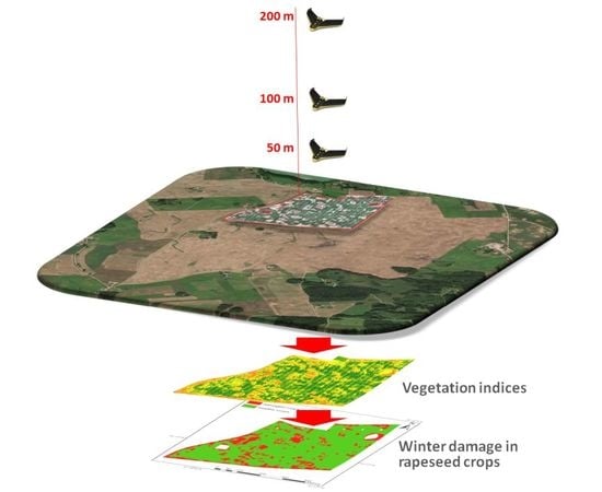
The experiment was carried out to analyze the possibility of using UAV-based multispectral imagery in the detection of damaged rapeseed after winter and the estimation of the damage area. The experiment was carried out in cooperation with an insurance company. Figure 1 shows the scheme of the experiment performed. Data were registered during three test flights on different flight heights in order to evaluate the influence of image spatial resolution. Each time, remote sensing data were acquired in four spectral bands, namely green, red, red edge, and near infrared, which were used to calculate tested vegetation indices. RGB images were acquired and combined with high-resolution spectral data, which were later used for manual preparation of reference data. Training samples were obtained during the field campaign.

In the methodology, there were a few crucial elements which are described in this section. Firstly, selected indices were tested to evaluate their usefulness in further analysis. The important part of the experiment was to delineate technical roads and replace those areas with a mean value from neighborhoods to exclude the effect of machinery influence (technical roads) on estimating damage. Another issue in the experiment was to define the influence of spatial resolution of the multispectral data on the obtained results.

2.1. Test Area and Data Used

For the planned tests, a 34 ha parcel with a rapeseed field was selected. It is situated in Olecko County in Northern Poland (Figure 2). This region is well known for its low temperatures and harsh climate throughout the year, hence, it was chosen for this experiment on the detection of winter crop damage. The winter of 2016/2017 in this region was characterized by high variability of weather conditions, with alternate periods of frost and thaw. During the period of severe frosts (from −12 to −27 °C) there was a thin layer of snow of several centimeters. This caused winter damage, which was confirmed during a field inspection.

The testing data were acquired with the use of an eBee UAV equipped with a Sequoia multispectral camera. This allowed for the acquisition of data in four different spectral bands: green (530–570 nm), red (640–680 nm), red edge (730–740 nm), and near infrared (770–810 nm). Three flights were performed on 20 April 2017, at three different altitudes of 50, 100, and 200 m above the ground. This resulted in images with three different spatial resolutions—ground sampling distances (GSD) of 5, 10, and 20 cm, respectively. This allowed us to assess the impact of spatial resolution on the imagery in the detection of a crop’s health when undamaged by frost. The overlapping of successive images along a flight strip (endlap) was 80%, and the overlap between flight strips (sidelap) was 70%. Flights were carried out in midday hours (12:00 p.m.–2:00 p.m.), with a cloudless or slightly cloudy sky. Wind speed was 1–2 m/s, air temperature was 5–6 °C, and humidity was 32–37%. The visibility was 35.5–43.8 km.

The orientation of images was performed in Pix4DMapper Pro software (Pix4D SA, Switzerland). This software allows the user to select the appropriate calculation template. For multispectral data calculation, the AG (agriculture) multispectral template is preferred. The program automatically recognizes the camera, retrieves its parameters from the database, groups the images into the appropriate spectral bands, and enables them to be calibrated. A useful feature of the Sequoia camera is that it can measure the amount of irradiance coming from the sun for each image and for each band with the sunshine sensor. This enables the user to take irradiance into account and normalize the value of the images amongst themselves. In the orientation process, self-calibration with 15 ground control points (control and check points) measured with a GNSS receiver was also performed to give a final root mean square error (RMS) of aerial triangulation of 10 cm. The result of the images processed in Pix4DMapper Pro were reflectance orthomosaics.

Based on the orthomosaics generated from the collected images in four spectral bands, different vegetation indices were calculated, based on which further experiments were conducted. To perform the correct classification of healthy and damaged crops, 23 training fields were created using data from field inspection and verified on RGB images. The training fields contained information about the number of healthy plants over a surface of 1 square meter (Figure 3). This helped to describe the relationship between the vegetation indices values and the number of plants in a surface unit, which resulted in thresholds for image classification.

2.2. Selection of Vegetation Indices

The most important process in determining post-winter damage is the correct detection of areas where the crop has not grown properly, or where the plants have died. Remote sensing as a multidisciplinary technique is a tool with many indices, which can help test the health of plants and solve the problem of the value of compensation for farmers for damaged crops. The Sequoia camera was the equipment used on the UAV in this study and allowed recording in four spectral bands: green, red, red edge, and near infrared. As a result of a literature review, a set of vegetation indicators was identified for further analysis. Consequently, after preliminary tests, the final selection was based on three basic spectral indices of vegetation: NDVI, SAVI, and OSAVI. In addition, an interesting solution in the calculation of these indices was to replace the red channel with the red edge, which was supported by the multispectral camera used in the experiment. Such modification was carried out and three further indices were examined: NDVI_RE, SAVI_RE, OSAVI_RE.

The NDVI (normalized difference vegetation index) is one of the most basic and commonly used indices [39]. It is a measure of photosynthetic activity and determines the condition of the plant and its development stage. Plants absorb most of the red light that hits it while reflecting much of the near infrared light. When vegetation is dead or stressed it reflects more red light and less near infrared light. Based on these properties, NDVI is calculated as the normalized difference between the red and near infrared bands from an image. The basic formula for calculating the index value is as follows:

$$\mathrm{NDVI}=\frac{\mathrm{NIR}-\mathrm{RED}}{\mathrm{NIR}+\mathrm{RED}}$$

(1)

where NIR is the near infrared band value and RED is the red band value.

The SAVI (soil adjusted vegetation index) is a modification of the NDVI index [40]. Due to changes in the numerator and denominator of the typical NDVI equation (soil brightness correction factor), the SAVI index further improves the final result for the influence of the soil brightness. For this reason, it is used in situations where a large part of the crop is not covered with lush vegetation. Therefore, the beginning of the growing season appears to be an excellent time for examining the condition of plants using this index. The formula for calculating SAVI is as follows:

$$\mathrm{SAVI}=\frac{\left(1+\mathrm{L}\right)\ast \left(\mathrm{NIR}-\mathrm{RED}\right)}{\mathrm{NIR}+\mathrm{RED}+\mathrm{L}}$$

(2)

where L denotes the coverage of the vegetation area. In most cases, and particularly for the case of intermediate vegetation canopy levels, optimal results are achieved using L = 0.5. For this experiment, a value 0.5 was used during the tests.

The OSAVI (optimized soil adjusted vegetation index) was developed by Rondeaux et al. (1996) [41] and was first presented in the work entitled “Optimized Soil Adjusted Vegetation Index”. This index is a modification of the SAVI that has been optimized for agricultural monitoring. It is more sensitive to changes in plant condition than the original SAVI and does not need a priori knowledge of the soil type. A value of 0.16 as the soil adjustment coefficient was selected as the optimal value to minimize variation with soil background. The formula for calculating OSAVI is as follows:

$$\mathrm{OSAVI}=\frac{\mathrm{NIR}-\mathrm{RED}}{\mathrm{NIR}+\mathrm{RED}+0.16}$$

(3)

In addition to the above three spectral indices, their modifications were tested in which the red channel was replaced by red edge. By analyzing spectral reflectance properties for plants in red edge wavelength, we can observe quick changes in reflection and can thus expect to see more discreet differences between healthy and damaged plants. To test this premise, NDVI_RE, SAVI_RE, and OSAVI_RE indices were calculated. The application of such indices with a modified channel has been discussed previously [42,43].

The correctness of damage recognition by the vegetation index was examined using training fields measured during a field inventory with the participation of insurance specialists. Twenty-tree sites were surveyed with an area of approximately 1 square meter and the condition of the plants was determined in their range. These fields were then characterized by experts as to whether they would qualify for compensation or if the plants in the field area were healthy. A training field was also specified that could be treated as two classes on the border: damaged and healthy crops. The training fields were ranked according to the condition of the plants. After calculating the mean values of the tested indices for each training field, the values obtained were compared with the reference from the field inventory. The threshold value was established based on the training fields which, according to experts, were found not to meet the conditions for granting compensation. Based on the healthy training field, threshold values for each index were used to classify (or not) training fields for compensation. All training fields were verified with an expert in the field. Their correctness was ensured so the outlier fields were eliminated in defining the thresholds. The threshold value was calculated as the mean value from the lowest mean value of the index for an accepted healthy crop training field and the highest mean value of the index for an accepted damaged crop training field. A comparison of results for training fields with defined thresholds is shown in Figure 4. As can be seen, the training fields were characterized by differentiation of the values of the vegetation indices. The highest standard deviation was noted in the fields with healthy plants, and the lowest in damaged areas. The greatest variability of the index values was related to the occurrence of plants of different sizes and condition. Training field no. 9 recorded higher NDVI and SAVI values due to the presence of weeds; furthermore, in training field no. 11, there were 10 healthy, well-developed plants, which also resulted in higher NDVI values.

Based on the selected thresholds, referring to each index, Figure 5 illustrates the errors in training fields, verified by inspection of the field. The red areas represent the test fields that, according to specialists, should be classified as damaged areas. The green areas represent fields without visible frozen influence. The threshold shown by a horizontal line in Figure 4 determined the correctness of interpretation for each training field: red areas should be below the threshold and green above. If the situation is reversed, it means that tested index does not work properly. After summarizing the errors, the top 3 results were finally selected, i.e., NDVI, OSAVI, and OSAVI_RE, to carry out further experiments.

In addition, considering the training fields, it is clear that the worst results were obtained for field no. 21. This was a unique area with healthy but very small plants (significant influence of the soil background). This suggests that the accepted threshold method may be sensitive to the stage in which the plants are grown, and results in slight over detection of damaged areas.

2.3. Elimination of Road Influence

Regardless of the selected vegetation index, the influence of technical roads is clearly visible on the classification results. The classification of technical roads, which are visible as traces of tires on a part of the field in poor condition, could have a big impact on the final results of detection, because this area should not be included in the calculation of the area of rapeseed damaged by frost.

The main insurer’s condition applied to an area for reimbursement is that the area of a detected polygon must cover some minimum area (i.e., larger than 100 m²). Therefore, many smaller objects are removed from the analysis. However, small isolated damaged areas are sometimes related to technical roads, which can result in detection of one bigger area, and are thus mistakenly detected as an area eligible for reimbursement. To prevent such situations, it was decided to work on rasters without the influence of roads on the reimbursement area.

For this purpose, road detection was conducted, based on compositions consisting of NDVI and green, red, and red edge channels. Object-based classification was performed in eCognition software for each dataset (data with spatial resolution equal to 5, 10, and 20 cm). In such a classification, information about spectral values, object shape, and extent were used. This resulted in three different road images, one for each spatial resolution of 5, 10, and 20 cm. Detected road images differed significantly from one another. The most precise and complete images came from images of 5 cm, and the worst from the lowest resolution (see Figure 6).

The biggest problems with areas of roads are presented in Figure 7, where there is no visible border between road and bare soil, which is why some tires traces were not detected. However, these places do not need to be detected because they do not cause the described problem of connecting polygons. Subsequently, a road mask was subtracted from the index rasters and the resulting holes were replaced with a mean value from corresponding cells (see Figure 7). Thus, the negative influence of technical roads on the final results of classification and detection of regions for reimbursement was reduced.

2.4. Approaches for Classification

The detection of damaged areas was performed using three different vegetation indices (NDVI, OSAVI, OSAVI_RE) in three different classification approaches, which were used to avoid the influence of technical roads on the result of winter damage crop estimation. The first method was a simple object-based classification to delineate the areas eligible for reimbursement. The main assumption behind this method was that it should appropriately suit borders of reference polygons which represent real situations and were vectorized without the generalization of polygons.

The second and third approach exploited pixel-based classification with thresholds. Index images were intersected with grids of cell sizes of 1 × 1 m and 5 × 5 m. For cells, a mean value of the index was assigned, and each cell was classified and merged with corresponding cells with the same class, creating homogenous regions. Thus, the resulting polygon geometry was simplified. By using those two approaches, we could also simulate a decrease in the resolution of input data.

In every approach, objects larger than 100 m² were finally recognized as detected damages. However, smaller regions lying within 5 m of other suspected damaged objects were also used, if the sum of their area was bigger than 100 m².

The possibility of proper detection of crops damaged by frost was examined using many variants. The influence of road elimination was examined, in addition to using a vegetation index for detection and spatial resolution of collected data. This resulted in 42 variants.

2.5. Accuracy Assessment

To estimate the accuracy of the final indications of which areas in each variant were eligible for reimbursement, a reference image was created by vectorization of damaged crops on an orthomosaic (see Figure 8).

The results were compared with reference areas by creating an error matrix which allowed for calculating such parameters as producer’s accuracy (PA, completeness), user’s accuracy (UA, correctness), F1-score, and overall accuracy (OA) [44,45]. The F1-score is the harmonic mean of precision and sensitivity and is usually used as an accuracy measure of a dichotomous model [45], so it is suitable for one-class delineation. In compensation assessment, the accurate area size of detected damage is much more important for the insurance company than its position, so another parameter was also used. This was the basic ratio of detected damaged areas to the reference area, and for the purpose of this study we named it “area index” (AI).

3. Results

The results of all variants for damaged rapeseed detection are presented in

Table A1. The results of all variants within the experiment, assessed by producer’s accuracy (PA) and user’s accuracy (UA) for class damaged crops, and area index (AI), F1-score, and overall accuracy (OA) of classification for damaged crops and healthy crops.

	Resolution	5 cm					5 cm
	Approach	Grid 1 × 1					Grid 5 × 5
	Index	UA	PA	AI	F1	OA	UA	PA	AI	F1	OA
without influence of roads	NDVI	83%	93%	113%	0.88	94%	78%	87%	111%	0.82	92%
	OSAVI	80%	93%	116%	0.86	94%	76%	87%	114%	0.81	92%
	OSAVI_RE	71%	93%	131%	0.81	91%	68%	88%	129%	0.77	89%
with influence of roads	NDVI	73%	96%	131%	0.83	92%	73%	90%	123%	0.81	91%
	OSAVI	69%	96%	138%	0.80	91%	70%	90%	129%	0.79	90%
	OSAVI_RE	65%	95%	146%	0.77	89%	65%	90%	139%	0.75	88%
	Resolution	10 cm					10 cm				10 cm
	Approach	Grid 1 × 1					Grid 5 × 5				Object-Based
	Index	UA	PA	AI	F1	OA	UA	PA	AI	F1	OA	UA	PA	AI	F1	OA
without influence of roads	NDVI	82%	93%	113%	0.87	95%	78%	86%	111%	0.82	92%	80%	92%	115%	0.86	94%
	OSAVI	84%	91%	108%	0.87	95%	79%	84%	106%	0.81	92%	81%	90%	110%	0.85	94%
	OSAVI_RE	77%	92%	120%	0.84	93%	73%	86%	117%	0.79	91%	76%	89%	117%	0.82	92%
with influence of roads	NDVI	74%	96%	130%	0.84	92%	73%	90%	123%	0.81	91%	63%	96%	153%	0.76	88%
	OSAVI	75%	94%	126%	0.83	92%	75%	94%	126%	0.83	92%	64%	94%	146%	0.76	88%
	OSAVI_RE	72%	94%	130%	0.82	91%	70%	88%	126%	0.78	90%	73%	91%	126%	0.81	91%
	Resolution	20 cm					20 cm
	Approach	Grid 1 × 1					Grid 5 × 5
	Index	UA	PA	AI	F1	OA	UA	PA	AI	F1	OA
without influence of roads	NDVI	79%	94%	118%	0.86	94%	78%	86%	111%	0.82	92%
	OSAVI	80%	92%	115%	0.86	94%	76%	86%	113%	0.81	92%
	OSAVI_RE	79%	90%	114%	0.84	93%	76%	85%	112%	0.80	92%
with influence of roads	NDVI	76%	100%	131%	0.86	94%	73%	89%	121%	0.80	91%
	OSAVI	77%	93%	121%	0.84	93%	74%	87%	118%	0.80	91%
	OSAVI_RE	78%	91%	117%	0.84	93%	75%	86%	115%	0.80	91%

in Appendix A. Figure 9 illustrates the comparison of the overall accuracy, the F1-score, and AI for all variants of the experiment. The visual effect of the classification for selected variants is presented in Figure 10.

Most variants of classification allow detection of winterkill with OA above 90% (Figure 9a). UA and PA ranged between 70–80% and 90–100%, respectively (Table A1 in Appendix A). This means that the algorithm detects almost every polygon from our reference set but also mistakenly indicates other areas (overestimation). The poorer result in UA may indicate some mistakes in the reference set, which was difficult to vectorize objectively in a field, and because the algorithm may overestimate the detection of crop losses, which is confirmed by the area of damage often exceeding 110% to 130% (Figure 9c). However, it should be noted that the overestimation relates to transition areas, which are inherently difficult to clearly separate (see Figure 11). Generally, the best results were achieved using OSAVI and NDVI indices (the highest UA, OA, and F1-score values). The highest accuracy (measured by F1-score and OA) with the smallest overestimation of the area of losses in crops (AI) was obtained for a spatial resolution of 10 cm. The worst results (low OA and F1, and high AI) were obtained for OSAVI_RE, using images with GSD = 5 cm. The area for compensation was overestimated by 29–31%, which may be caused, for example, by inaccuracies in the georeference of an image with a spatial resolution of 5 cm.

In the next section, a deeper analysis of the influence of road removal, the spatial resolution of collected images, and the vegetation indices used in this experiment is provided.

4. Discussion

4.1. Influence of Road Removal and Approaches in Damage Detection

As expected, road removal was a crucial step for obtaining better results. It allowed us to avoid many errors in the classification of smaller objects connected with roads (see Figure 7). It also prevented the incorrect enlargement of detected losses by incorporating road areas in detected polygons.

The negative influence of roads is highlighted in all three approaches on 10 cm input rasters. In both the second (grid 1 × 1 m) and the third (grid 5 × 5 m) approaches, each index increases UA by 3–5 percentage points, with a slight decrease of PA (around three percentage points) with only one exception of a higher outlier (10 percentage points for OSAVI in grid 5 × 5 m) (see Table A1 in Appendix A). The direction of changes in the first approach (object-based) are similar. The decrease of PA is on the same level as in other approaches, however, the increase in UA equals 17 percentage points on OSAVI and NDVI indices, and only two percentage points for OSAVI _RE, which is due to a much bigger UA value for this index before road removal (73–63% and 64% for NDVI and OSAVI, respectively). Although the differences in the range of increase of UA are high, the discrepancies in the final results between approaches 1 and 2 do not exceed three percentage points. This is also reflected by the area index (see Figure 11). The area index’s values decrease in all three approaches after using the road removal technique. For OSAVI and NDVI indices, the difference is over two times higher in the object-based approach, but for OSAVI_RE, the decrease is on the same level as in the pixel-based approaches, which may be due to the fact that in the OSAVI_RE variant, technical roads are slightly less visible and are harder to distinguish in the images. This results in a lower number of roads that qualified as winter damage polygons.

The conducted analysis indicates that without removing road influence, object-based classification is a significantly worse method for proper winter damage detection. The generalization that is performed during the process of averaging the cell value in approaches 2 and 3 (resolution of grids 1 and 5 m, respectively), causes the rejection of some fraction of roads, which is not the case in the object-based approach because it provides a more precise classification. Because of this characteristic, a higher resistance to road influence in the OSAVI_RE index is most observable in the object-based scenario.

4.2. Influence of Spatial Resolution

The comparison of PA and UA for a 1 × 1 m grid with respect to vegetation indices is shown in Figure 12. Comparing NDVI results in this approach, we can assume that the smaller the GSD (ground sampling distance of obtained images), the better the results (an increase in the F1-score is observed). However, UA and PA values are almost equal for resolutions of 5 and 10 cm. The visible difference comes only at the 20 cm raster (a decrease of three percentage points in UA and 0.02 in F1-score value). In the case of the OSAVI index, we can confirm that results are slightly better on the 10 cm raster than 5 cm, but 20 cm still results in the worst outcome. The OSAVI_RE index trend is contrary to NDVI, with most of the indicator’s values rising with decreasing pixel size. In the second approach, a 20 cm input OSAVI_RE raster results in a F1-score value of 0.84 and an OA equal to 93% (Table A1 in Appendix A), which is only slightly worse than the results obtained from other indices. The detected damage area is also more similar to the reference data than in comparable variants. This information allows us to suppose that, with an increasing size of GSD, OSAVI_RE could be the best index to use in the whole process. Generally, it can be assumed that any tested spatial resolution of UAV-based imagery is enough for winter damage assessment for insurance purposes and there are few differences in terms of accuracy in the tested approaches in the detection of these areas without plants.

For the results obtained in the described experiments with NDVI, decreasing the size of GSD provided better results, while the research of Candiago et al. (2015) [9] showed that the use of such a high resolution can be a problem when applying algorithms originally developed for aerial and satellite data. In this paper, three approaches were tested with OBIA, or resampling to grid sizes of 1 × 1 m and 5 × 5 m, which limited this problem.

The highest overall accuracy of detection wais achieved using the NDVI index on two different input data sets with 5 and 20 cm GSD (see Table A1 in Appendix A). For rasters with 10 cm resolution, the better choice was the OSAVI index, which was clearly confirmed in the majority of variants. However, the difference between the overall accuracy of damage detection using NDVI and OSAVI is not significant (1–2%). The usefulness of the NDVI vegetation index to determine the vegetation fraction (the percentage of green vegetation per unit of ground surface) and the number of plants per unit of ground surface is confirmed by the results of other authors (among others [19,22]). In our experiment, the results related to OSAVI_RE index are slightly better.

4.3. Influence of Vegetation Index Used

Figure 13 presents the results of damage detection for different vegetation indices in the case of the three approaches. Analysis of this figure allows us to draw a few crucial conclusions. Firstly, we can state that the producer’s accuracy is stable in all three approaches regardless of chosen vegetation index as input data for classification. Its values vary from 0 to 3 percentage points in the same approach. However, approach 3 (grid 5 × 5 m) provides smaller absolute PA (around 85%) and UA (77%) values than the other approaches (mean values of 91% and 80%, respectively). This is mostly the result of much stronger generalization in this approach. Secondly, it is observed that there are significant differences in the user’s accuracy between the chosen indices in all three approaches.

In each variant, OSAVI_RE has the lowest value. OSAVI provides slightly better UA than NDVI (difference of 1–2 percentage points), but NDVI compensates this disparity with slightly higher PA values. Analysis of the overall accuracy (see Table A1 in Appendix A) indicates that those two indices are the same, however, the area of damage in all three approaches is 5 percentage points better for OSAVI than NDVI. The difference in the F1-score is only 0.01. Nonetheless, for data with a resolution of 5 cm (for both approaches) and 20 cm (for the third approach), the results indicate that NDVI is slightly better than OSAVI (see Table A1 in Appendix A).

5. Conclusions

The experiments performed demonstrate that low-altitude remote sensing can be used for the assessment of damaged areas in the case of insurance compensation. The case study used multispectral UAV images for the damage detection of rapeseed caused during winter. Data were acquired in April, when plant vegetation starts. This is the most important period in estimating damage since it directly exposes the effect of the winter period on vegetation. The presented methodology includes selecting possible vegetation indices, ground sampling resolutions, and approaches for technical road influence elimination, which can be used as an effective alternative for direct measurements in a field that currently are often used during the refurbishment process.

The analysis of GSD images (in the range of 5–20 cm) demonstrates a relatively small (a few percentage points) influence on the obtained results of winterkill detection. The best approximation of the area of the winter damage to crops was obtained using images with GSD of 10 cm. Results for most variants indicate that there is no need to acquire data with a higher resolution than 10 cm. This is a crucial conclusion for UAV application when the size of the area and the GSD of the images are considered within mission planning

The conclusion of the presented experiment is of great practical importance because cameras with four spectral channels (R, G, B, NIR) are becoming increasingly popular and relatively inexpensive. This provides the possibility to choose various vegetation indices appropriately for the analyzed crop and the purpose of the study related to the monitoring of the crop condition. The best results were obtained using NDVI and OSAVI vegetation indices; however, results from other indices were not significantly worse.

Referring to the utilization of the red edge spectral band, an optimized Soil-Adjusted Vegetation Index with the use of the red edge channel instead of the red channel is the most resilient index to the negative influence of technical roads, which is crucial when road detection cannot be conducted. The optimized soil-adjusted vegetation index with red edge channel (OSAVI_RE) may be the best for crop condition monitoring using lower spatial resolution data.

During tests, it was also necessary to develop and implement elimination of technical roads in calculations of rapeseed area damaged with frost. Including the detected area in the classification helps in the reliable calculation of the area for compensation. Without removing road influence, object-based classification is a significantly worse method, but elimination of road influence can be processed using both object- and pixel-based approaches. In tests with NDVI and OSAVI, overestimation of 10–30% was noticed for calculations without the elimination of the impact of roads, and all of the remote sensing-based approaches in all experiments were characterized by overestimation of at least a few percent considering the Area Index.

The implementation of the presented solutions for delimiting areas for refurbishment in the comprehensive damage estimation method, which also includes periodic monitoring and time analysis, can significantly improve the compensation process, and provide it with scientific certainty for obtained results.