Anchor-free Convolutional Network with Dense Attention Feature Aggregation for Ship Detection in SAR Images

Abstract

In recent years, with the improvement of synthetic aperture radar (SAR) imaging resolution, it is urgent to develop methods with higher accuracy and faster speed for ship detection in high-resolution SAR images. Among all kinds of methods, deep-learning-based algorithms bring promising performance due to end-to-end detection and automated feature extraction. However, several challenges still exist: (1) standard deep learning detectors based on anchors have certain unsolved problems, such as tuning of anchor-related parameters, scale-variation and high computational costs. (2) SAR data is huge but the labeled data is relatively small, which may lead to overfitting in training. (3) To improve detection speed, deep learning detectors generally detect targets based on low-resolution features, which may cause missed detections for small targets. In order to address the above problems, an anchor-free convolutional network with dense attention feature aggregation is proposed in this paper. Firstly, we use a lightweight feature extractor to extract multiscale ship features. The inverted residual blocks with depth-wise separable convolution reduce the network parameters and improve the detection speed. Secondly, a novel feature aggregation scheme called dense attention feature aggregation (DAFA) is proposed to obtain a high-resolution feature map with multiscale information. By combining the multiscale features through dense connections and iterative fusions, DAFA improves the generalization performance of the network. In addition, an attention block, namely spatial and channel squeeze and excitation (SCSE) block is embedded in the upsampling process of DAFA to enhance the salient features of the target and suppress the background clutters. Third, an anchor-free detector, which is a center-point-based ship predictor (CSP), is adopted in this paper. CSP regresses the ship centers and ship sizes simultaneously on the high-resolution feature map to implement anchor-free and nonmaximum suppression (NMS)-free ship detection. The experiments on the AirSARShip-1.0 dataset demonstrate the effectiveness of our method. The results show that the proposed method outperforms several mainstream detection algorithms in both accuracy and speed.

1. Introduction

Ship detection in synthetic aperture radar (SAR) images plays a significant role in many aspects, such as maritime management, information acquisition and so on. It has received much attention in recent years. Traditional ship detection methods are usually composed of the following steps: (1) sea–land segmentation; (2) data preprocessing; (3) prescreening; and (4) false alarm elimination [1,2,3,4]. On this basis, researchers have developed a variety of methods, mainly including clutter modeling-based [2,5], multi-resolution-based [6,7], domain transformation-based [8,9], handcraft feature-based [10,11] and polarimetric information-based methods [12]. These traditional methods are suitable for detecting strong scattering targets in low-resolution SAR images. With the improvement of SAR imaging resolution, the accuracy, robustness and efficiency of these methods are difficult to be guaranteed due to their complex detection process [13,14,15,16]. Therefore, it is necessary to develop methods with high accuracy and fast speed for ship detection in high-resolution SAR images.

Recently, deep-learning-based methods, especially deep convolutional neural networks (DCNNs), have achieved better accuracy and faster speeds over traditional methods in computer vision, thanks to the powerful automated feature extraction ability of DCNN. Due to the superior performance, they have been widely studied by researchers [17,18,19,20]. For example, Ren et al. [21] put forward to use the region proposal network (RPN) in Faster-RCNN to replace the selective search algorithm, which largely improves the detection efficiency and accuracy. The single-shot multibox detector (SSD) by Liu et al. [22] and you only look once (YOLO) by Redmon et al. [23] regress the location and the category of the targets directly through the features by the feature extraction network without extracting candidate regions, further improving the detection efficiency. In the task of ship detection in SAR images, DCNN-based methods have also achieved good performance. In previous research, researchers tried to combine DCNN into the four steps of traditional ship detection (sea–land segmentation, data preprocessing, prescreening and false alarm elimination). For example, Liu et al. [24] proposed to conduct sea–land segmentation and ship detection using pyramid features extracted by DCNN. Zhao et al. [25] proposed coupled convolutional neural networks (CNN) to extract candidate ship targets. In recent studies, to improve the detection efficiency and accuracy, researchers directly take origin SAR images as the input of DCNN, without sea–land segmentation or data preprocessing. In this way, the automatic feature extraction ability of DCNN can be fully utilized and ship detection can be accomplished end-to-end. For example, Zhao et al. [26] presented a ship detection method based on Faster-RCNN. They use DCNN to extract multiscale features directly from the original intensity map of SAR images, achieving automatic candidate determination and discrimination. Kang et al. [27] fused shallow and deep features of DCNN to combine contextual information from the origin SAR images for ship detection. Cui et al. [28] put forward to enhance the feature extraction ability of Faster-RCNN through dense connections and the attention mechanism. Gao et al. [29] combined spatial attention blocks and split convolution blocks in RetinaNet for multiscale ship detection in SAR images. Chen et al. [30] embedded an attention module into the feature extraction process of DCNN to conduct ship detection in complex scenes of SAR images. Zhang et al. [31] proposed a DCNN based on depth-wise separable convolution to realize high-speed SAR ship detection. Chang et al. [32] presented an improved YOLOv3 to conduct real-time SAR ship detection.

The above DCNN-based methods all adopt an anchor-based mechanism for ship detection, where they have to manually set different sizes and aspect ratios of anchors before training and testing. The detection is accomplished by predicting the category of the anchors and the errors between anchors and real bounding boxes. Some disadvantages exist in these anchor-based methods: (1) The sizes and aspect ratios of the anchors need to be carefully configured in advance. Nevertheless, it is difficult to make this optimal, leading to performance degradation. For example, in [33], the average precision of the detection results drops 4% because of the defective anchor settings. (2) The anchors are fixed once they have been configured, which makes it difficult for the detector to deal with the situation that the target scales change greatly. For different data sets, it is also necessary to readjust the anchor settings. (3) The densely distributed anchors lead to massive computational costs in the training process, and the nonmaximum suppression (NMS) postprocessing algorithm [34] is required to screen out duplicate detections.

To overcome the above problems, researchers develop alternative detection methods. These methods conduct detection by regressing the key points of targets, and hence anchors are not necessary. For instance, Law et al. [35] proposed to predict the bounding box of the targets by regressing the upper left corner and the lower right corner of the target. Tian et al. [36] encode the target position by predicting 4D vectors pixel by pixel to achieve anchor-free detection. Yang et al. [37] use deformable convolution to predict a group of key points for each target. The location of the target is acquired according to the minimum bounding box of the key points. In recent studies, for anchor-free SAR ship detection, researchers used fully convolutional networks to segment the ship targets from the SAR images. For example, Fan et al. [38] propose to use an improved U-net architecture to conduct pixel-wise segmentation of the ship targets in polarimetric SAR images. Mao et al. [39] perform efficient ship detection by using a simplified U-net. However, anchor-free ship detection by segmentation requires pixel-wise labeling of the SAR data, which is very time-consuming. In this paper, to overcome the drawbacks of anchor-based methods, we introduce an anchor-free detector in our method, namely center-point-based ship predictor (CSP). CSP achieves anchor-free ship detection by predicting the center-point of the target and regressing the size of the target at the same time. There is no pre-set anchor or massive anchor-related calculation. In addition, the detection results can be obtained without using an NMS postprocessing algorithm, thus further improving the computational efficiency.

In addition, a large number of parameters leads to high computational costs for most of the DCNN-based detection algorithms. In order to improve the detection efficiency, they usually detect targets on the feature maps with the lowest resolution and the strongest semantic information. However, this may cause missed detections for small targets. A large number of parameters also leads to the overfitting problem when the system is trained on the SAR data set with limited labeled samples. To alleviate this problem, researchers train the DCNN models by fine-tuning the models pretrained on the ImageNet [40] dataset. However, the pretrained models and the models for SAR ship detection have great differences in the training objective functions and target distributions, which may bring the learning bias. Therefore, in this paper, we adopt a lightweight feature extractor based on MobileNetv2 [41] to extract multiscale ship features, which improves the detection speed and the generalization performance of the network. For the multiscale features extracted by the feature extraction network, we propose a novel feature aggregation scheme called dense attention feature aggregation to strengthen the feature reuse and further improve the generalization ability. Combining the above ideas, our method can be trained directly on the SAR data set without pretraining. High-resolution features with multiscale information can be obtained by dense attention feature aggregation (DAFA) for anchor-free ship detection.

To sum up, to overcome the defects existing in current DCNN-based SAR ship detection methods, in this paper, we first use a lightweight feature extractor based on MobileNetV2 to extract multiscale features of the origin SAR images. By replacing the standard convolution with the depth-wise separable convolution, the network parameters are effectively reduced and the computational efficiency is greatly improved. Next, to improve the detection performance for multiscale targets, especially small ship targets, we propose a novel feature aggregation scheme, i.e., DAFA, to deeply fuse the extracted multiscale features and generate high-resolution features. In DAFA, through the dense connections and the iterative feature fusions of adjacent scale features, the representation ability of the features is enhanced. The feature reuse strategy is utilized to improve the generalization ability of the model. We embed an attention module squeeze and excitation (SCSE) into DAFA to exert attention over the salient features of the targets and reduce the background clutters. Finally, the deeply-fused high-resolution features are fed as input towards the anchor-free detector CSP. The three subnetworks of CSP predict the center-points, sizes and downsampling errors of the ship targets, respectively, to achieve anchor-free and NMS-free ship detection. The effectiveness of our method is evaluated on the AirSARShip-1.0 data set consisting of Gaofen-3 SAR images [42]. The experimental results show that our proposed method can achieve better detection accuracy and speed than other mainstream DCNN-based ship detection methods.

The rest of the paper is arranged as follows: Section 2 introduces our proposed method in detail, which mainly includes the lightweight feature extractor, dense attention feature aggregation and center-point ship predictor. The experimental results on the AirSARShip-1.0 data set are given in Section 3 to quantitatively and qualitatively evaluate the effectiveness of our method. In Section 4, we discuss the influence of the network’s width on the detection performance and further validate the components’ effectiveness. Section 5 gives the conclusion.

2. Materials and Methods

Figure 1 illustrates the detailed architecture of our proposed method, which can be divided into three parts from left to right: the lightweight feature extractor, dense attention feature aggregation (DAFA) and the anchor-free ship detector, namely center-point-based ship predictor (CSP). Firstly, the input SAR image is processed by a convolution layer with stride = 2 to reduce the size of features and expand the receptive field. Then, features of four different scales {C₁, C₂, C₃, C₄} are extracted through the four convolution stages of the lightweight feature extractor. These multiscale features are gradually refined in DAFA through dense iterative connections, which generates the refined multiscale features {P₁, P₂, P₃, P₄}. Next, the high-resolution features P₄ are successively fused with {P₁, P₂, P₃} by 2×, 4× and 8× upsamplings. We embed an attention block, which is the SCSE block, into the upsampling process to emphasize the salient features of the ship targets, suppress the background clutters and optimize the representation ability of the features. Through DAFA, the high-resolution feature F_out is obtained and fed into CSP for further anchor-free ship detection. CSP is mainly composed of three sub-branches: (1) ship center estimation branch for predicting the location of the ship centers. (2) Ship size regression branch for estimating the length and width of ship targets, and (3) center offset regression branch for compensating the downsampling errors. Anchor-free and NMS-free ship detection is achieved by merging the results of these three branches. In this section, we will introduce the three parts of our method, respectively, in detail.

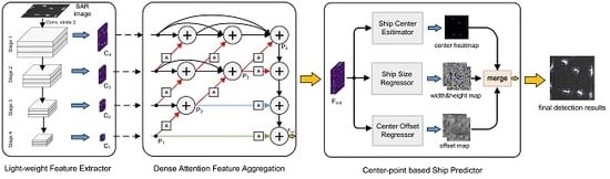
2.1. Lightweight Feature Extractor Based on MobileNetV2

In DCNN, high-level features usually have a larger receptive field, and stronger semantic information. Therefore, they are suitable for detecting large targets. On the other hand, shallow features usually contain less semantic information while maintaining a higher resolution. So, they are more capable of detecting small targets. For improving the performance of multiscale ship detection in SAR images, researchers extract multilevel features using DCNN [43,44]. However, detection based on multiscale features usually leads to an increase in parameters and computational costs. The generalization ability of DCNN in SAR data also declines due to the increase in parameters. In this paper, in order to reduce the parameters of DCNN and improve the detection speed, we adopt the lightweight feature extractor based on MobileNetV2 to extract the multiscale features of SAR images. The specific structure of the lightweight feature extractor is illustrated in

Table 1. Structure of the MobileNetV2-based feature extractor, where t denotes the dimension expansion ratio of the features after the first 1 × 1 convolution layer in inverted residual blocks (IRB); c represents the number of output channels; s stands for the stride; and n indicates to stack the operation for n times.

Stage	Input	Operation	t	c	n	s	Output Name
1	512 × 512 × 3	Conv2d	-	32	1	2	-
	256 × 256 × 32	IRB	1	16	1	1	-
	256 × 256 × 16	IRB	6	24	2	2	C4
2	128 × 128 × 24	IRB	6	32	3	2	C3
3	64 × 64 × 32	IRB	6	64	4	2	-
	32 × 32 × 64	IRB	6	96	3	2	-
	32 × 32 × 96	IRB	6	160	3	1	C2
4	16 × 16 × 160	IRB	6	320	1	2	C1

.

As given in Table 1, the structure of the lightweight feature extractor can be mainly divided into four convolution stages. Each stage outputs one feature with different scales, represented by {C₁, C₂, C₃, C₄}. Each stage is composed of several conventional convolution layers or inverted residual blocks (IRB). The parameter settings of these operations are also shown in Table 1. Among them, t denotes that the first 1 × 1 convolution layer and IRB increases the dimension of the features by t times; c represents the number of output channels; s stands for the stride, the resolution of the features reduces to half when s = 2; and n indicates to stack the operation for n times. The specific introduction for IRB can be referred to [41]. It mainly consists of two 1 × 1 convolutions and a 3 × 3 depth-wise separable convolution (DSConv). By replacing the standard convolution with a combination of a depth-wise convolution and a point-wise convolution, the computational cost of DSConv is reduced by a factor of $(k^2+d_o)/(d_o{k}^2)$ [41,45]. $d_0$ and $k$ represent the number of output channels and the kernel size, respectively. For instance, the computational cost of 3 × 3 DSConv is about 1/9 of the standard 3 × 3 convolution, which greatly improves the efficiency of the network.

In addition, the width of the network, i.e., the dimension of the feature maps, largely determines the number of parameters. For data sets of different sizes, reasonable adjustments on the width of the network can effectively reduce the parameters and improve the generalization ability. There are a total of seven kinds of IRB in the feature extractor. The numbers of their output channels are {16, 24, 32, 64, 96, 160, 320}. We use the following rules to adjust the output channels of IRB (the width of the network):

$$\begin{array}{l}t=\max (d,\lfloor \lfloor \alpha c_{old}+d/2\rfloor /d\rfloor \times d)\\ c_{new}=\{\begin{array}{cc}t+d& t<0.9\alpha c_{old}\\ t& t\ge 0.9\alpha c_{old}\end{array}\end{array}$$

(1)

where $c_{old}$ denotes the original dimension of output features and $c_{new}$ denotes the adjusted dimension of output features. d represents a divisor. In this paper, we set d = 8 in all the experiments. $\alpha$ is the adjustment ratio. A typical range for $\alpha$ is (0,2). $\lfloor \cdot \rfloor$ indicates rounding down operation. According to Equation (1), the width of the network can be adjusted proportionally to $\alpha$. At the same time, the new numbers of channels satisfy that: (1) They can be divided by d; (2) and all of them are greater than $0.9\alpha c_{old}$. For example, given $\alpha =0.5$, the numbers of the output channels of seven IRBs are adjusted to {8, 16, 16, 32, 48, 80, 160}. In the discussion section of this paper, we further discuss the influence of the width of the network on detection performance.

2.2. Dense Attention Feature Aggregation

In this paper, we propose a novel feature fusion scheme called dense attention feature aggregation (DAFA) to deeply fuse multiscale features by the feature extractor. Through DAFA, high-resolution features with multiscale information are obtained for further ship detection. To introduce DAFA in detail, this section is divided into two parts. In the first part of the section, the design idea of DAFA is derived by analyzing the weakness of several existing methods. In the second part, we describe the basic feature fusion unit of DAFA. The SCSE block is introduced to enhance the representation ability of the features by emphasizing the salient features of the targets and suppressing the background clutters.

2.2.1. Ideas of Dense Attention Feature Aggregation

In order to detect multiscale ship targets, especially small ship targets in SAR images, it is of vital importance to obtain high-resolution features with multiscale information. The high-resolution features C₄ by the feature extractor are not capable for the ship detection because of its limited receptive field and shallow semantic meanings. Therefore, a well-designed feature fusion process is necessary to combine multiscale information and obtain high-resolution features. To show the design ideas of our proposed feature aggregation process, Figure 2 illustrates different kinds of feature aggregation schemes. We will introduce the design ideas of our method by analyzing the weaknesses of several existing methods and making improvements over these methods.

Figure 2a shows a classic feature fusion structure [46], namely long skip connections (LSC). Among the multiscale features {C₁, C₂, C₃, C₄} by the feature extractor, C₁ is the smallest but with richest semantic information. LSC gradually upsamples C₁, and fuses it with the other three features, C₂, C₃ and C₄, through long skip connections. This process can be described as follows:

$$P_n=L(C_1,C_2,\cdots ,C_n)=\{\begin{array}{cc}{C}_1& ifn=1\\ L(S(C_1,C_2),\cdots ,C_n)& otherwise\end{array},$$

(2)

where $C_i$ represents the feature maps of the $i_{th}$ scale output by the feature extractor, $P_i$ represents the refined feature maps of the $i_{th}$ scale, $L(\cdot )$ represents the LSC feature aggregation process, and $S(\cdot )$ represents the feature fusion block. In the feature fusion block, low-resolution features are upsampled to the same resolution as the high-resolution features. Then they are fused by element-wise addition. n is the number of multiscale feature maps by the feature extractor. In our model, $n=4$.

LSC is able to produce high-resolution features while the fused results are relatively coarse due to the skip connections. The fusion process shown in Figure 2b is improved by introducing iterative short connections [47]. This process is called iterative deep aggregation (IDA), which can be expressed by Equation (3):

$$P_n=I(C_1,C_2,\cdots ,C_n)=\{\begin{array}{cc}\begin{array}{c}{C}_1\\ S(P_1,C_2)\\ S(P_{n-1},I(C_2,\cdots ,C_n))\end{array}& \begin{array}{c}ifn=1\\ ifn=2\\ otherwise\end{array}\end{array},$$

(3)

where $I(\cdot )$ denotes the IDA process.

The iterative aggregation of features enhances feature representation and combines multiscale information from coarse to fine. However, drawbacks still exist in this kind of fusion scheme. There only exist short connections between feature maps, which leads to the problem of gradient vanishing. Recent studies have shown that adding long skip connections to the network is helpful for detection. It mitigates the gradient vanishing problem and the overfitting problem by feature reuse [48,49]. Inspired by this idea, we propose to combine short connections and long connections to form dense connections. The derived dense iterative aggregation (DIA) process is shown in Figure 2c. The fusion process can be expressed iteratively by Equation (4):

$$P_n=T(C_1,C_2,\cdots ,C_n)=\{\begin{array}{cc}\begin{array}{c}{C}_1\\ S(P_1,C_2)\\ S(P_{n-1},C_n,T(C_2,\cdots ,C_n),T(C_3,\cdots ,C_n),\cdots ,T(C_{n-1},C_n))\end{array}& \begin{array}{c}ifn=1\\ ifn=2\\ otherwise\end{array}\end{array},$$

(4)

where $T(\cdot )$ represents the DIA process. Different scales of refined features {P₁, P₂, P₃, P₄} are produced through this feature aggregation process.

To further enhance the semantic information in the high-resolution feature maps, we add a high-resolution feature fusion path to combine information from the refined multiscale features{P₁, P₂, P₃}. As shown in Figure 2d, P₁, P₂, P₃ are, respectively, upsampled 2, 4 and 8 times and successively fused with the high-resolution feature P₄. The high-resolution fusion path can be calculated through Equation (5):

$$F_{out}=H(P_n,P_{n-1},\cdots ,P_1)=\{\begin{array}{cc}{P}_n& ifn=1\\ H(S(P_n,P_{n-1}),\cdots ,P_1)& otherwise\end{array},$$

(5)

where $H(\cdot )$ denotes the high-resolution feature fusion path. The new feature aggregation scheme is called dense hierarchical aggregation (DHA) in this paper. Through DHA, we obtain the high-resolution feature map $F_{out}$ enhanced with multiscale information.

In addition, recent studies show that the attention mechanism is helpful for improving the performance of SAR ship detection [28,29,30]. Inspired by the idea, we embed an attention block, i.e., SCSE block into the upsampling process. SCSE is used to emphasize the salient target features and suppress the background clutters in the high-level features, and thus improve the localization ability of the fused features. As shown in Figure 2e, the feature aggregation process embedded with SCSE is called dense attention feature aggregation (DAFA), which is shown in Figure 2e. The whole process can be computed by Equations (2) and (3), while $S(\cdot )$ here represents the attention-based feature fusion block, which will be described in detail in the next section.

2.2.2. Attention-Based Feature Fusion Block

In the above aggregation process, features of different scales are aggregated through dense connections and iterative feature fusions. As the basic unit of the aggregation process, the feature fusion block plays an important role in combining information from multiscale features. The effectiveness of the feature fusion block consequently has a great impact on the detection performance. Recent researches show that the attention mechanism is able to enhance the salient features of the targets and hence improve the representation ability of the fused features. For example, Cui et al. [28] embed an attention block into the upsampling process to emphasize the salient information of the multiscale ship targets, thus improving the detection performance of the network. Gao et al. [29] introduced an attention block into the network to reduce the information loss in the dimension reduction.

Inspired by the ideas, we introduce an attention block, namely the spatial and channel squeeze and exception block (SCSE) [50] into the feature fusion block. In the multiscale feature fusion process, the high-level features contain stronger semantic information thus have a greater influence on the identification and the localization of the ship targets. SCSE is applied to improve the representation ability of the fused features by strengthening the salient features and suppressing the background clutters in the high-level and strong semantic features. The new feature fusion block embedded with SCSE is called the attention-based feature fusion block (AFFB). In addition, the deformable convolution is used in AFFB to replace the standard 3 × 3 convolution. The deformable convolution learns the sampling offsets to enforce it to focus more on the interesting targets. In the object detection task, it has been proved to be effective in improving the localization ability of the network [37,51]. The structure of AFFB is shown in Figure 3. Features from the higher-level are first processed by SCSE, then upsampled to the same resolution as other features. Next, these features are fused through element-wise addition after the deformative convolutions. Finally, a convolution layer is used to refine the fused features.

Next, we will introduce the SCSE block in detail. The diagram of SCSE is shown in Figure 4a. SCSE exerts spatial and channel attention over the high-level feature maps through spatial squeeze and excitation (SSE) and channel squeeze and excitation (CSE). They, respectively, generate the spatial attention maps and the channel attention maps. The values of the elements in the generated attention maps are within the range of [0, 1]. The generated attention maps are then multiplied with the input features. They weigh the features to preserve the salient features and suppress noise. Finally, the attention-enhanced features are obtained through element-wise addition. The overall process of SCSE can be described by Equation (6):

$$F_A=A_S\odot F+A_C\otimes F,$$

(6)

where $F\in {ℝ}^{\tilde{H}\times \tilde{W}\times \tilde{C}}$ represent the input features, $A_S\in {\left[0,1\right]}^{\tilde{H}\times \tilde{W}\times 1}$ denotes the spatial attention map generated by SSE, $A_C\in {\left[0,1\right]}^{1\times 1\times \tilde{C}}$ denotes the channel attention map generated by CSE, $F_A\in {ℝ}^{\tilde{H}\times \tilde{W}\times \tilde{C}}$ represent the output features, $\otimes$ denotes the multiplication operation on the corresponding channels and $\odot$ denotes the multiplication operation on the corresponding positions.

SSE block is designed to spatially emphasize the salient features of the ship targets. As shown in Figure 4b, SSE first squeezes the dimension of the input features $F\in {ℝ}^{\tilde{H}\times \tilde{W}\times \tilde{C}}$ by $1\times 1$ convolution. The function of the $1\times 1$ convolution is to integrate information across different channels and generate activation values. Then the spatial attention map $A_C\in {\left[0,1\right]}^{1\times 1\times \tilde{C}}$ is acquired by applying the sigmoid function. The sigmoid function is used to map the activation values to [0, 1]. The process of SSE is as follows:

$$A_S=\sigma (Con{v}_{1\times 1}(F))$$

(7)

where $Con{v}_{1\times 1}$ and $\sigma (\cdot )$ represent $1\times 1$ convolution and sigmoid function, respectively.

The CSE block is introduced to stress the important semantic embedding among different channels of the input features. The detailed structure of CSE is shown in Figure 4c. Firstly, global pooling (GP) is used to incorporate the spatial information of each channel. GP produces a single value for each channel that represents the information contained in the channel. These values are then combined to form a feature vector. Next, two $1\times 1$ convolutions are used to perform dimension reduction and dimension increase to this feature vector based on the squeeze and excitation principle [52]. Finally, the channel attention vector is generated by applying a sigmoid function. The channel attention vector is then used to weigh the different channels of the input features, so as to selectively enhance the important semantic information contained in different channels. The process of CSE can be represented by Equation (8):

$$A_C=\sigma (Con{v}_{1\times 1}[Con{v}_{1\times 1}(GP(F))]),$$

(8)

where GP denotes global pooling operation, $Con{v}_{1\times 1}$ represents $1\times 1$ convolution and $\sigma (\cdot )$ is the sigmoid function.

Together, the propagation process of AFFB can be shown in Equation (9):

$$F_{fused}=Dcon{v}_{3\times 3}[\underset{\mathrm{fe}ature\mathrm{from}\mathrm{scale}(\mathrm{i}-1)}{\underbrace{Dcon{v}_{3\times 3}(Upsample(SCSE(F_{(i-1)0})))}}\oplus \underset{features\mathrm{from}\mathrm{scale}\mathrm{i}}{\underbrace{{\displaystyle {\sum }_{j=1}^{n}Dcon{v}_{3\times 3}(SCSE(F_{ij})})}}],$$

(9)

where $F_{ij}$ is the i_th feature from scale j, Dconv represents the deformable convolution, Upsample stands for the upsampling operation, and $\oplus$ denotes element-wise addition operation. Through AFFB, the salient features of the ship targets are enhanced in the high-level features, and then densely fused with adjacent low-level features. The final fused features are obtained by element-wise addition.

2.3. Center-Point-Based Ship Predictor

Among the classic DCNN-based detection algorithms, most of them rely on the pre-set anchors of different sizes and aspect ratios for detection. The concept of anchors (or anchor boxes) in the field of DCNN-based target detection is firstly presented in [21]. In the anchor-based detection methods, the targets are detected by predicting the errors between the pre-set anchors and the actual bounding boxes, as shown in Figure 5a. Some disadvantages exist in this kind of detection methods, such as the difficulty in their adaptability to large scale-variations of the targets, the difficulty of the parameter optimization of anchors and high computational costs. Therefore, an anchor-free detector is introduced in our method, which is the center-point-based ship predictor (CSP). As shown in Figure 5b, CSP achieves anchor-free ship detection by simultaneously predicting the center-points and the sizes of the ship targets in a fully convolutional way. Moreover, by applying a 3 × 3 Max-pooling operation, the duplicate detections can be ruled out, which is more efficient than the NMS algorithm.

The detailed structure of CSP is shown in Figure 6. It is composed of three sub-branches: the center estimation, the size regression and the offset regression branches. The input SAR image $I\in R^{H\times W\times 3}$ is first processed by the feature extractor and DAFA. Then high-resolution features $F\in {ℝ}^{\tilde{H}\times \tilde{W}\times C}$ by DAFA are fed towards these three branches, where $\tilde{H}=H/4$ and $\tilde{W}=W/4$. After the operations of a $3\times 3$ convolution and an $1\times 1$ convolution, the ship center estimation branch produces the ship center estimation heatmap $\widehat{Y}\in {[0,1]}^{\tilde{H}\times \tilde{W}\times 1}$ that indicates the locations of the ship centers; the size regression branch outputs the ship width and length prediction maps $\widehat{S}\in {ℝ}^{\tilde{H}\times \tilde{W}\times 2}$ that predict the width and length of ship targets; and the offset regression branch generates the offset prediction maps $\widehat{O}\in {ℝ}^{\tilde{H}\times \tilde{W}\times 2}$, which compensate the downsampling errors in the x- and y-axis.

To train the center estimation branch of CSP, we first generate the ground truth in terms of the center-points of the ship targets. For image $I$, let $(x_1^{(k)},y_1^{(k)},x_2^{(k)},y_2^{(k)})$ denote the bounding box of the k_th ship target in the image. Then, the center-point of the k_th ship target can be calculated as $c_k=(\frac{x_1^{(k)}+x_2^{(k)}}{2},\frac{y_1^{(k)}+y_2^{(k)}}{2})\in {ℝ}^2$. We compute the coordinate of this center-point on the downsampled features F by ${\tilde{c}}_k=\lfloor c_k/4\rfloor$. Next, we place all the ship centers on the ground truth heatmap $Y\in {[0,1]}^{\tilde{H}\times \tilde{W}\times 1}$ by using a 2D Gaussian kernel $Y_{xy}=\exp (-({(x-{\widehat{c}}_{kx})}^2+{(y-{\widehat{c}}_{ky})}^2)/2{\sigma }_a{}^2)$, where ${\sigma }_a$ is the standard deviation that adaptively changes according to the target size [31]. When two Gaussian centers overlap, we take the larger value on every overlapped position. Given that the center estimation branch outputs the ship center estimation heatmap $\widehat{Y}\in {[0,1]}^{\tilde{H}\times \tilde{W}\times 1}$, the pixel-wise focal loss for ship center prediction is calculated as follows:

$$L_{\text{h}m}=-\frac{1}{N}{\displaystyle \sum _{xy}\{\begin{array}{cc}{(1-{\widehat{Y}}_{xy})}^{\alpha }\log ({\widehat{Y}}_{xy})& if{Y}_{xy}=1\\ {(1-Y_{xy})}^{\beta }{({\widehat{Y}}_{xy})}^{\alpha }\log (1-{\widehat{Y}}_{xy})& otherwise\end{array}}$$

(10)

where α and β are the hyperparameters of the focal loss, we set α = 2 and β = 4 in the experiments that result in the best outcomes; N is the number of ship targets in image I, which is used to normalize the positive samples of focal loss in each image; Y_xy and ${\widehat{Y}}_{xy}$ denote the elements of the ground truth map and the center estimation heatmap, respectively. Focal loss improves the detection performance by reducing the weights of easy samples in loss calculation. It makes the model focus more on hard samples during the training [33].

For each ship k in image I, the size regression branch regresses its size $s_k=(x_2^{(k)}-x_1^{(k)},y_2^{(k)}-y_1^{(k)}$ at the corresponding center-point of the ship. The size regression branch outputs the ship length and width prediction maps $\widehat{S}\in {ℝ}^{\tilde{H}\times \tilde{W}\times 2}$. We use L1 loss to calculate the regression loss of the branch:

$$L_{size}=\frac{1}{N}{\displaystyle \sum _{k=1}^N\left|{\widehat{S}}_k-s_k\right|},$$

(11)

where ${\widehat{S}}_k$ and $s_k$ denote the actual and predicted sizes of the k_th ship target, respectively.

The prediction maps are downsampled by four times compared to the original input image. Discretization errors are introduced when we are calculating the downsampled center coordinates through ${\tilde{c}}_k=\lfloor c_k/4\rfloor$. In order to compensate for these errors, we use the offset regression branch to predict the discretization errors. We use the same L1 loss as the size regression branch:

$$L_{off}=\frac{1}{N}{\displaystyle \sum _{k=1}^N\left|{\widehat{O}}_{{\tilde{c}}_k}-(\frac{c_k}{R}-{\tilde{c}}_k)\right|},$$

(12)

where ${\widehat{O}}_{{\tilde{c}}_k}$ is the predicted center discretization error of the k_th ship target, and R is the downsampling rate, which is 4 in our method. It needs to be noticed that the supervision is only conducted on each ship center ${\tilde{c}}_k$.

Finally, to jointly train the three branches, we calculate the overall loss by the weighted sum of the above three losses, as Equation (13):

$$L_{cdet}=L_{hm}+{\beta }_{size}{L}_{size}+{\beta }_{off}{L}_{off},$$

(13)

where ${\beta }_{size}$ and ${\beta }_{off}$ are the hyperparameters representing loss weights. As suggested in [51], ${\beta }_{size}=0.1$ and ${\beta }_{off}=1$ are set in all our experiments.

During testing, we obtain the detection results by integrating the outputs of the three branches. Firstly, a 3 × 3 Max-pooling is applied to the ship center estimation map to generate a group of detections for the ship centers. The 3 × 3 Max-pooling can effectively eliminate the duplicate detections. It can replace the NMS postprocessing algorithm in faster speed due to the GPU acceleration. Let $\widehat{C}={\left\{({\widehat{x}}_i,{\widehat{y}}_i)\right\}}_{i=1}^n$ denote the estimated ship centers. The coordinates of the i_th ship center is represented by $({\widehat{x}}_i,{\widehat{y}}_i)$. Then the detected bounding boxes can be expressed by Equation (14):

$$\begin{array}{cc}\hfill \widehat{B}=\left\{(x_{{\min }_i},y_{{\min }_i},x_{{\max }_i},y_{{\max }_i}{)}_{i=1}^n\right\}& =({\widehat{x}}_i+\delta {\widehat{x}}_i-{\widehat{w}}_i/2,{\widehat{x}}_i+\delta {\widehat{x}}_i+{\widehat{w}}_i/2,\hfill \\ \hfill & {\widehat{y}}_i+\delta {\widehat{y}}_i-{\widehat{h}}_i/2,{\widehat{y}}_i+\delta {\widehat{y}}_i+{\widehat{h}}_i/2),\hfill \end{array}$$

(14)

where $\widehat{B}$ represents the set of the detected bounding boxes; $\delta {\widehat{x}}_i$ and $\delta {\widehat{y}}_i$ are the predicted discretization errors of the i_th ship center in x and y directions, respectively; and ${\widehat{w}}_i$ and ${\widehat{h}}_i$ are the predicted width and height of the i_th ship target, respectively.

3. Results

In this section, we implement experiments on the AirSARShip-1.0 data set to evaluate the effectiveness of our method. First, the AirSARShip-1.0 data set and the experimental settings will be described in detail. Then, the evaluation metrics for quantitative comparison are introduced. Next, we evaluate the effectiveness of the DAFA by comparison experiments. Finally, we compare our methods with several DCNN-based ship detection algorithms, the qualitative and quantitative results are given to validate the performance of our method.

3.1. Data Set Description and Experimental Settings

In this paper, to evaluate the effectiveness of our method, experiments are carried out on a large-scene and high-resolution SAR ship detection data set AirSARShip-1.0 [53]. AirSARShip-1.0 consists of 31 single-polarized SAR images acquired from Gaofen-3. The polarization mode of these SAR images is HH. The imaging modes include the spotlight and strip. The resolution varies from 1 m to 3 m. Most of the image sizes are 3000 × 3000 pixels (one of them is 4140 × 4140 pixels). In the experiments of this paper, 21 of the 31 SAR images of the dataset are used as the train-val (training and validation) set, and the remaining 10 images are used as the test set. We then randomly split the train-val set into the training set and the validation set with the proportion of 7:3. Considering the limitation of the GPU memory, we divide the large-scene SAR images into 500 × 500 slices for training and testing. For those ships that are truncated by slicing, we keep the bounding boxes whose area exceeds 80% of the original bounding box, otherwise, the bounding boxes are discarded. The training set only consists of slices that contain ship targets. In the test set, we conduct the detection on all the slices whether they contain the ship targets or not. Finally, we augment the training set by 90-degree rotation. After augmentation, there are a total of 512 image slices with a size of 500 × 500 in the training set. A large-scene image of the AirSARShip-1.0 is shown in Figure 7a, which contains inshore and offshore scenes and different scales of ship targets. Several image slices are shown in Figure 7b–e. Figure 7b mainly shows inshore scenes and small ship targets while Figure 7c shows the offshore scenes. In Figure 7d, there are strong land clutters around the ship targets. The ship targets shown in Figure 7e are very small compared to other images. In summary, it can be seen that the data set includes both inshore and offshore scenes, and the size of ships varies greatly.

The training hyperparameters of our method are set as follows: we randomly initialize the parameters of our models, without using the ImageNet pretrained models. We train the three parts of our model end-to-end with labeled data. We use Adam optimizer [54] as the training optimizer, and the weight decay of which is set to 0.0005. The learning rate is 0.001, and the number of minibatch samples is set to four. We train the models for 200 epochs in total. The learning rate drops by 10 times at the 120th and 180th epoch. The width adjustment ratio mentioned in Section 2.1 is set to 0.5 in all our experiments.

The experiments are implemented using the deep learning framework Pytorch [55], and carried out on a platform configured with 32G memory, an Intel Xeon L5639 CPU and a Tesla K20c GPU for training and testing. The system of the experiment platform is Ubuntu 18.04.

3.2. Evaluation Metrics

Three widely used metrics are adopted in this paper to quantitatively evaluate the performance of the models, including the precision–recall (PR) curve (PR), average precision (AP) and f₁-score. As the name suggests, the PR curve takes recall as the abscissa axis and precision as the ordinate axis. The more areas the PR curve covers, the better the model performs. The precision measures the correctness of the detection results, calculated by the fraction of the true positives in the detected positive samples. The recall indicates the completeness of the detection results, which can be computed by the fraction of the true positives in all the positive samples. The calculation of these two metrics can be described by Equation (15):

$$\{\begin{array}{c}\mathrm{Precison}=\frac{N_{TP}}{N_{TP}+N_{FP}}\\ \mathrm{Recall}=\frac{N_{TP}}{N_{TP}+N_{FN}}\end{array},$$

(15)

where $N_{TP}$ represents the number of the correctly detected targets. $N_{FP}$ indicates the number of the nonship targets that are wrongly detected; $N_{FN}$ denotes the number of the undetected ship targets.

There is a contradiction between precision and recall. When increasing one of the two metrics, the other will decline. To address the contradiction, we introduce the f₁-score that combines these two metrics to comprehensively evaluate the detection performance. The f₁-score metric can be computed as follows:

$$f_1\text{-}\mathrm{score}=2\frac{\mathrm{precision}\times \mathrm{recall}}{\mathrm{precision}+\mathrm{recall}},$$

(16)

The f₁-score measures the detection performance of the model with a single-point threshold. The AP metric is adopted to evaluate the global detection performance under different thresholds. It is measured by the area under the PR curve, which can be expressed as follows:

$$\mathrm{AP}={\displaystyle {\int }_0^1\mathrm{P}\left(\mathrm{R}\right)d\mathrm{R}},$$

(17)

3.3. Effectiveness of Dense Attention Feature Aggregation

In order to improve the localization ability of the network for multiscale ship targets, especially small ship targets, we propose the feature aggregation scheme DAFA mentioned in Section 2.2. To generate high-resolution features and mitigate the overfitting problem, the specially designed dense connections and the attention-augmented upsampling are introduced in DAFA. Here, we verify the effectiveness of DAFA by conducting several carefully designed comparison experiments. To be specific, we set comparison experiments with different feature aggregation schemes, which are: (1) Long Skip Connections (LSC) [46] as shown in Figure 2a; (2) Iterative Deep Aggregation (IDA) [47] as shown in Figure 2b; (3) Dense Iterative Aggregation (DIA) as shown in Figure 2c; (4) Dense Hierarchical Aggregation (DHA) as shown in Figure 2d; (5) Dense Attention Feature Aggregation (DAFA) as shown in Figure 2e. In the experiments, other hyperparameters required in training and testing are set to be the same. In order to quantitatively evaluate the effectiveness of DAFA,

Table 2. The quantitative detection performance of different feature aggregation schemes.

Methods	Precision (%)	Recall (%)	f1-Score (%)	AP (%)
LSC	77.86	75.17	76.49	77.13
IDA	79.70	77.93	78.81	80.49
DIA (ours)	82.98	80.69	81.82	82.96
DHA (ours)	82.07	84.26	83.15	85.34
DAFA (ours)	85.03	86.21	85.62	86.99

gives the detailed detection results of different feature aggregation schemes.

It can be seen from Table 2 that DAFA achieves the best performance in precision, recall, f₁-score and AP, reaching 85.03%, 86.21%, 85.62% and 86.99%, respectively. For LSC, IDA and DIA, the overall detection performance measured by f₁-score and AP is gradually improved. It demonstrates that the iterative refinement and dense connections are helpful for ship detections. DHA achieves higher performance than DIA, which implies that the high-resolution feature fusion path further strengthens the semantic information and improves the representation ability of the high-resolution features. For DHA and DAFA, the results show that the introduction of SCSE improves f₁-score and AP by 2.5% and 1.7%. It indicates that SCSE can effectively emphasize the salient features in high-level features. The enhanced high-level features are helpful for strengthening the representation ability of the fused features and further optimize the detection performance of the network.

The PR curves are illustrated in Figure 8a to comprehensively show the effectiveness of these aggregation schemes. It is shown that the PR curve of LSC lies at the innermost, indicating that its detection performance is the worst. The PR curve of IDA shows improvement, proving that the iterative connections can produce finer features than long skip connections. The PR curve of DIA lies lower than that of IDA, demonstrating that dense connections can help achieve better performance by feature reuse strategy. The PR curve of DHA lies lower than that of DIA, showing that the high-resolution feature fusion path is able to optimize the detection performance by fusing features with larger receptive fields and stronger semantic information. The PR curve of DAFA is at the highest, which suggests that the attention mechanism can effectively strengthen the localization accuracy and semantic meaning in the high-level features, and thus improve the representation ability of the fused features.

In addition, comparisons of the number of the parameters and the detection speed are revealed in Figure 8b, where params denotes the number of all parameters (M) in the network, and times is obtained by computing the average time (ms) for detecting a SAR image slice on the test set. As shown in Figure 8b, DHA has a relatively small increase (only 0.12M) in the parameter amount compared with LSC. A lot of element-wise addition fusions are introduced in the aggregation process, which results in an increase of 9 ms in test time. From Figure 8b, we can also find that the parameters of DAFA embedded with SCSE increase very little (only about 0.01M), while the detection time is increased by 7 ms. It indicates that the number of parameters of the SCSE block is small, and the computational cost is relatively large but acceptable.

In Figure 9, we visualize the detection results on several SAR image slices for comparison. Figure 9a shows the ground truth, in which the real ship targets are marked with purple rectangles. Figure 9b–f shows the detection results of DAFA, DHA, DIA, IDA and LSC, in which the detected ship targets are marked with green rectangles. The false alarms and missed targets can be located with the reference of Figure 9a. As shown in Figure 9f, the detection results of LSC are the worst among these methods. There are more false alarms and missed ship targets in both inshore and offshore scenes. IDA also has some false alarms and missed targets in different scenes according to Figure 9e. Compared with these two methods, DIA in Figure 9d has less missed targets in the inshore scene. DHA further improves the detection results compared to DIA. The missed targets in the offshore scene are reduced. The comparison of the above detection results demonstrates that dense connections and iterative feature fusions can effectively improve the localization ability of the network for a variety of scenes. The high-resolution feature fusion process further optimizes the detection results by combining multiscale semantic information. In Figure 9b, it can be seen from the results of DAFA that the false alarms in the land area further reduce. It indicates that SCSE is able to suppress the background clutters in the high-level features, optimize the feature fusion process and improve the detection performance.

3.4. Comparison with Other Ship Detection Methods

In this section, we will compare our method with other DCNN-based ship detection methods. The traditional ship detection methods are suitable for detecting low-resolution targets with strong scattering, while for high-resolution SAR images, the DCNN-based methods greatly surpass these methods in accuracy and efficiency even with limited training samples [21,45,53]. Hence, to verify the effectiveness of our method, we compare our method with several other state-of-the-art DCNN-based methods, which are introduced as follows:

• Faster-RCNN [21]: Faster-RCNN is a classic deep learning detection algorithm, and is widely studied in the ship detection of SAR images [39,49]. Faster-RCNN employs the region proposal network (RPN) to extract target candidates for coarse detection. Then, the detection results are refined by further regression.
• RetinaNet [33]: RetinaNet is a deep learning algorithm based on the feature pyramid network (FPN) for multiscale target detection. The focal loss is proposed to improve the detection performance for hard samples.
• YOLOv3 [56]: YOLOv3 is a real-time detection algorithm, where the feature extraction network is carefully designed to realize the high-speed target detection.
• FCOS [36]: Among the above three deep learning detection algorithms, the predefined anchors are used to help predict targets in training and testing. FCOS is a recently proposed anchor-free detection algorithm. It achieves the anchor-free detection by regressing a 4D vector representing the location of the targets pixel by pixel.
• Reppoints [37]: Reppoints is also a newly proposed anchor-free detection algorithm, which locates a target by predicting a set of key points and transforming them into the predicted bounding box.

Except that YOLOv3 is implemented with the Darknet framework [57], we implement most of the comparison experiments using the MMDet framework [58] based on Pytorch. Among the above comparison experiments, YOLOv3 uses the darknet-53 with 53 convolution layers as the feature extraction network, and all the other methods adopt ResNet-50 [59] with 50 convolution layers as the feature extraction network. The training and testing hyperparameters are set according to the suggestions in MMDet or Darknet. An early stopping strategy is used to reduce the overfitting problem. The quantitative detection results of these methods are presented in

Table 3. The quantitative detection performance of several deep convolutional neural network (DCNN)-based ship detection algorithms.

Methods	Precision (%)	Recall (%)	f1-Score (%)	AP (%)
YOLOv3	63.87	68.28	66.00	64.65
FCOS	67.07	77.24	71.79	68.84
Reppoints	65.24	84.07	73.47	73.98
RetinaNet	72.12	82.07	76.77	79.00
Faster-RCNN	73.49	84.14	78.46	78.43
Ours	85.03	86.21	85.62	86.99

.

From Table 3, we can see that the overall performance of our method measured by f₁-score and AP surpass other methods by more than 5%. It proves the effectiveness of our method. Among other detection methods, YOLOv3 has the worst detection performance, both f₁-score and AP are less than 70%. The anchor-free based methods FCOS and Reppoints achieve better performance than YOLOv3, but the overall performance is relatively poor compared to other anchor-based methods. The detection performance of RetinaNet and Faster-RCNN is better than that of YOLOv3, FCOS and Reppoints. Both of the AP values are close to 80%, achieving 79.00% and 78.43%, respectively. The reason why anchor-based methods perform better than peer anchor-free methods is that the pre-set anchors actually incorporate the prior information of the target sizes. Therefore, it reduces the difficulty in training on the SAR data set with limited training samples. In order to take advantage of the anchor-free mechanism and generalize well on the SAR data set, we combine a lightweight feature extractor and the feature reuse strategy into the anchor-free detection. As a result, compared to other comparison methods, our method is more effective for detecting multiscale ship targets in the SAR images.

The PR curves of the detection methods are drawn in Figure 10a. It can be observed that the PR curve of the YOLOv3 method is at the innermost, indicating that its detection performance is the worst. The PR curve of FCOS is fuller than YOLOv3′s. The PR curve of Reppoints shows improvement over those of the above two methods, but still lies at the inner side of Faster-RCNN and RetinaNet’s. The PR curve of our method lies at the outermost, showing that it has the best global performance for ship detection. In summary, the results verify the superior performance of our method.

Figure 10b compares the number of the parameters and detection speed of these DCNN-based detection methods. As shown in Figure 10b, YOLOv3 has the largest number of parameters (61.5M), because of its 53-layer feature extraction network. However, the detection time of YOLOv3 is the shortest (9.9 ms), showing superior efficiency. It is due to its specially designed network structure and the highly efficient framework that this algorithm is implemented on. However, it should be noticed that although achieving high efficiency, the performance of YOLOv3 is very poor with the AP of 0.6465. Among other methods, our method reaches the highest detection speed (33 ms), while the detection times of Reppoints, FCOS, RetinaNet and Faster-RCNN takes 75 ms, 53 ms, 72 ms and 50 ms, respectively. It demonstrates the high efficiency of our method. Besides, the weight of our method (0.83M) is far lighter than all other methods. In summary, the above results show that our method is efficient in computation and light in storage, thanks to the lightweight feature extractor and the feature reuse strategy. Next, to further validate the performance of our method, we present the detection results of different DCNN-based methods on real SAR images in Figure 11 and Figure 12.

In Figure 11, detection results on several SAR image slices qualitatively show the performance of these methods. Figure 11a gives the ground truth and Figure 11b–g shows the results of our method, RetinaNet, Faster-RCNN, Reppoints, FCOS and YOLOv3, respectively. Image slices in the first three rows are composed of offshore scenes, and the latter three include the inshore scenes. In Figure 11g, a lot of missed detections occur in both inshore and offshore scenes of the YOLOv3′s detection results. In Figure 11f, the missed detections are reduced in the results of FCOS, but still, many ship targets remain undetected. The results of FCOS in Figure 11e show few missed detections in the offshore scene, but false alarms appear in some land areas due to the land clutter. In Figure 11d, Faster-RCNN mistakenly detects the weakly-scattered ghost targets on the sea surface as ship targets in the second image, a small ship target is undetectable in the third image and false alarms appear in the land areas. In Figure 11c, RetinaNet is prone to generate false alarms and missed detections in the strong scattering area, resulting in inaccurate detection results. In Figure 11b, the results of our method are more accurate than other methods, with few false alarms and missed detections in both inshore and offshore scenes. Therefore, the results demonstrate that our method has superior detection performance than other comparison methods.

Figure 12 shows a comparison between the detection results of different methods on a large-scene SAR image in the test set. This large-scene SAR image mainly includes offshore ships. There are strong clutters in the inshore scenes which might lead to false alarms. We can see that there appear few false alarms and missed targets in the offshore scenes in the results of our method, and the false alarms are suppressed in the inshore scenes as well. For Faster-RCNN, a lot of false alarms occur in the inshore scenes. The detection results of RetinaNet have fewer false alarms than that of Faster-RCNN in the inshore scenes, but the false alarms in the offshore scenes increase. In Figure 12d, the results of Reppoints have serious false alarm problems both in the inshore and offshore scenes. In Figure 12e, missed detections happen in the offshore scenes for FCOS, and there are also some false alarms in the inshore scenes. In Figure 12f, the YOLOv3 method has a serious problem of missed detection in the offshore scenes, which greatly degrades the quality of the detection results. The comparison of these detection results further proves the effectiveness of our method.

4. Discussion

4.1. Influence of the Network’s Width

The network’s width has a key influence on the number of parameters and the detection speed of the network. A smaller width may lead to fewer parameters and better generalization ability. However, if the width is too small, the fitting ability of the network will be deficient and the detection performance will be degraded as a result. In this paper, due to the lightweight feature extractor and the feature reuse strategy used in DAFA, our method generalizes well in the SAR data set and does not rely on the pretrained model for training. Therefore, in our method, we can freely adjust the network’s width to balance the generalization ability and the detection speed of the model. To show the influence of the network’s width, Figure 13 illustrates how the detection performance and efficiency of our method change in different widths.

We adjust the network’s width with the help of the adjustment ratio $\alpha$ described in Section 2.1. The results for different widths are acquired by conducting experiments on different $\alpha$. To be specific, we initially set $\alpha$ to 0.25 and increase it to two with a step of 0.25. Figure 13a shows the influence of the network’s width on the detection performance of the network. A small $\alpha$ indicates a smaller network width. We can see that AP reaches the highest when $\alpha =0.5$ and f₁-score reaches the highest when $\alpha =0.75$. When $\alpha$ is smaller than 0.5, the detection performance degrades greatly. When $\alpha$ is greater than one, the detection performance gradually drops. It implies that our method reaches the best generalization ability on the adopted SAR data set when $\alpha \in \left(0.5,0.75\right)$. Figure 13b gives the results of the number of parameters and the detection time for different widths of the network. We can observe that the number of the parameters increases exponentially as $\alpha$ increases. The detection time also gradually increases as $\alpha$ increases. To conclude, as the width of the network increases, the detection performance of the network first increases due to the improvement of the fitting ability, and then degrades because of the degradation of the generalization ability. The detection speed drops due to the increment of the number of the parameters. After balancing the performance and efficiency, we select $\alpha =0.5$ as the network’s width in all our experiments.

4.2. Validating the Effectiveness of Feature Map Visualization

In order to intuitively evaluate the effectiveness of DAFA, we visualized the intermediate feature maps in DAFA as shown in Figure 14a. We also visualize the feature maps of LSC in Figure 14b for comparison. In Figure 14, the corresponding feature maps of three SAR image slices are displayed in each aggregation stage. For the convenience of visualization, the feature maps of different scales are resized to the same size. The brighter colors represent stronger responses. It can be concluded from Figure 14 that: (1) With the decrease of resolution, the location accuracy of the targets declines, the semantic meaning of the features is strengthened and the strong land clutter is gradually suppressed; (2) In DAFA, the location accuracy of the targets is gradually improved because of the dense connections and the attention augmentation, while the results of LSC is more coarse due to the long skip connections; (3) The high-resolution feature fusion path in DAFA effectively combines semantic information from different scales and suppress the background clutters. The above observation demonstrates the effectiveness of DAFA to combine multiscale information and generate high-resolution features, thanks to the specially designed dense connections and SCSE.

To visually verify the effectiveness of the SCSE, some feature maps are visualized in Figure 15. Figure 15b shows the feature maps before processed by SCSE, and Figure 15c shows the feature maps output by SCSE. In the visualization results, the brighter colors denote greater activation values. By comparing Figure 15b,c, we can observe that the contrast between targets and the background is improved, and the position responses of the targets are more accurate. In the inshore scenes, we can see that the land clutters are effectively suppressed after SCSE. The above results indicate that SCSE can effectively enhance the salient features of the targets and suppress the background clutters.

5. Conclusions

To overcome several defects in current DCNN-based methods, in this paper, we have proposed a novel fully convolutional network for anchor-free ship detection in SAR images. The main contributions of this paper are as follows: (1) To overcome the weaknesses of the anchor-based detection methods, we adopted an anchor-free detector, i.e., CSP, to conduct anchor-free and NMS-free ship detection. CSP predicts the centers and sizes of the ship targets end-to-end without pre-set anchors, which make the ship detection process faster and more accurate. (2) To improve the generalization ability of DCNN in the SAR data set, we presented a novel feature aggregation scheme, i.e., DAFA, to deeply fuse the multiscale features. The feature reuse strategy by dense connections was introduced to alleviate the overfitting problem and improve the generalization ability. The SCSE attention block was embedded into DAFA to strengthen the representation ability of the fused features and thus optimize the detection performance. (3) To reduce the parameters in DCNN and improve the detection efficiency, we adopted a lightweight feature extractor based on MobileNetV2 to extract multiscale features directly from the single-polarized SAR images. The depth-wise separable convolution was used to replace the standard convolution, which helps achieve higher efficiency with fewer parameters. The experiments implemented on the AirSARShip-1.0 data set demonstrate that the dense connections, iterative feature fusions and the attention mechanism in DAFA effectively improve the performance of the anchor-free ship detection in SAR images. The results have also shown that the performance of our method surpasses other methods, further validating the effectiveness of our method.

References

1. Crisp, D. The State-of-the-Art in Ship Detection in Synthetic Aperture Radar Imagery; Australian Government, Department of Defense: Canberra, Australia, 2004; p. 115. [Google Scholar]
2. Ao, W.; Xu, F.; Li, Y.; Wang, H. Detection and discrimination of ship targets in complex background from spaceborne alos-2 sar images. IEEE J. Top. Appl. Earth Observ. Remote Sens. 2018, 11, 536–550. [Google Scholar] [CrossRef]
3. Huo, W.; Huang, Y.; Pei, J.; Zhang, Q.; Gu, Q.; Yang, J. Ship detection from ocean sar image based on local contrast variance weighted information entropy. Sensors 2018, 18, 1196. [Google Scholar] [CrossRef] [PubMed] [Green Version]
4. Schwegmann, C.P.; Kleynhans, W.; Salmon, B.P. Synthetic aperture radar ship detection using haar-like features. IEEE Geosci. Remote Sens. Lett. 2016, 14, 154–158. [Google Scholar] [CrossRef] [Green Version]
5. Ai, J.; Qi, X.; Yu, W.; Deng, Y.; Liu, F.; Shi, L. A new cfar ship detection algorithm based on 2-d joint log-normal distribution in sar images. IEEE Geosci. Remote Sens. Lett. 2010, 7, 806–810. [Google Scholar] [CrossRef]
6. Liu, N.; Cao, Z.; Cui, Z.; Pi, Y.; Dang, S. Multi-scale proposal generation for ship detection in sar images. Remote Sens. 2019, 11, 526. [Google Scholar] [CrossRef] [Green Version]
7. Zhang, F.; Wu, B. A scheme for ship detection in inhomogeneous regions based on segmentation of sar images. Int. J. Remote Sens. 2008, 29, 5733–5747. [Google Scholar] [CrossRef]
8. Tello, M.; López-Martínez, C.; Mallorqui, J.J. A novel algorithm for ship detection in sar imagery based on the wavelet transform. IEEE Geosci. Remote Sens. Lett. 2005, 2, 201–205. [Google Scholar] [CrossRef]
9. Tello, M.; Lopez-Martinez, C.; Mallorqui, J.J. Ship detection in sar imagery based on the wavelet transform. ESASP 2005, 584, 20. [Google Scholar]
10. Leng, X.; Ji, K.; Zhou, S.; Xing, X.; Zou, H. An adaptive ship detection scheme for spaceborne sar imagery. Sensors 2016, 16, 1345. [Google Scholar] [CrossRef] [Green Version]
11. Wang, C.; Jiang, S.; Zhang, H.; Wu, F.; Zhang, B. Ship detection for high-resolution sar images based on feature analysis. IEEE Geosci. Remote Sens. Letters 2013, 11, 119–123. [Google Scholar] [CrossRef]
12. Wang, C.; Wang, Z.; Zhang, H.; Zhang, B.; Wu, F. A polsar ship detector based on a multi-polarimetric-feature combination using visual attention. Int. J. Remote Sens. 2014, 35, 7763–7774. [Google Scholar] [CrossRef]
13. Ren, J. Ann vs. Svm: Which one performs better in classification of mccs in mammogram imaging. Knowl.-Based Syst. 2012, 26, 144–153. [Google Scholar] [CrossRef] [Green Version]
14. Zhang, T.; Zhang, X. High-speed ship detection in sar images based on a grid convolutional neural network. Remote Sens. 2019, 11, 1206. [Google Scholar] [CrossRef] [Green Version]
15. Kang, M.; Leng, X.; Lin, Z.; Ji, K. A Modified Faster R-CNN Based on CFAR Algorithm for SAR Ship Detection. In Proceedings of the 2017 International Workshop on Remote Sensing with Intelligent Processing (RSIP), Shanghai, China, 18–21 May 2017; pp. 1–4. [Google Scholar]
16. Fei, G.; Aidong, L.; Kai, L.; Erfu, Y.; Hussain, A. A novel visual attention method for target detection from sar images. Chin. J. Aeronaut. 2019, 32, 1946–1958. [Google Scholar]
17. Zhao, Z.-Q.; Zheng, P.; Xu, S.-T.; Wu, X. Object detection with deep learning: A review. IEEE Tran. Neural Netw. Learn. Syst. 2019, 30, 3212–3232. [Google Scholar] [CrossRef] [Green Version]
18. Yue, Z.; Gao, F.; Xiong, Q.; Wang, J.; Huang, T.; Yang, E.; Zhou, H. A novel semi-supervised convolutional neural network method for synthetic aperture radar image recognition. Cogn. Comput. 2019, 1–12. [Google Scholar] [CrossRef] [Green Version]
19. Gao, F.; Huang, T.; Sun, J.; Wang, J.; Hussain, A.; Yang, E. A new algorithm of sar image target recognition based on improved deep convolutional neural network. Cogn. Comput. 2019, 11, 809–824. [Google Scholar] [CrossRef] [Green Version]
20. Zhang, W.; Li, Q.; Wu, Q.J.; Yang, Y.; Li, M. A novel ship target detection algorithm based on error self-adjustment extreme learning machine and cascade classifier. Cogn Comput. 2019, 11, 110–124. [Google Scholar] [CrossRef]
21. Ren, S.; He, K.; Girshick, R.; Sun, J. Faster R-CNN: Towards real-time object detection with region proposal networks. In Advances in Neural Information Processing Systems; Morgan Kaufmann: San Mateo, CA, USA, 2015; pp. 91–99. [Google Scholar]
22. Liu, W.; Anguelov, D.; Erhan, D.; Szegedy, C.; Reed, S.; Fu, C.-Y.; Berg, A.C. Ssd: Single Shot Multibox Detector. In Proceedings of the European Conference on Computer Vision(ECCV), Amsterdam, The Netherlands, 8–16 October 2016; pp. 21–37. [Google Scholar]
23. Redmon, J.; Divvala, S.; Girshick, R.; Farhadi, A. You only look once: Unified, real-time object detection. In Proceedings of the IEEE Conference on Computer Vision and Pattern Recognition(CVPR), Las Vegas, NV, USA, 27–30 June 2016; pp. 779–788. [Google Scholar]
24. Liu, Y.; Zhang, M.-h.; Xu, P.; Guo, Z.-w. Sar ship detection using sea-land segmentation-based convolutional neural network. In Proceedings of the 2017 International Workshop on Remote Sensing with Intelligent Processing (RSIP), Shanghai, China, 18–21 May 2017; pp. 1–4. [Google Scholar]
25. Zhao, J.; Zhang, Z.; Yu, W.; Truong, T.-K. A cascade coupled convolutional neural network guided visual attention method for ship detection from sar images. IEEE Access 2018, 6, 50693–50708. [Google Scholar] [CrossRef]
26. Zhao, J.; Guo, W.; Zhang, Z.; Yu, W. A coupled convolutional neural network for small and densely clustered ship detection in sar images. Sci. China Inf. Sci. 2019, 62, 42301. [Google Scholar] [CrossRef] [Green Version]
27. Kang, M.; Ji, K.; Leng, X.; Lin, Z. Contextual region-based convolutional neural network with multilayer fusion for sar ship detection. Remote Sens. 2017, 9, 860. [Google Scholar] [CrossRef] [Green Version]
28. Cui, Z.; Li, Q.; Cao, Z.; Liu, N. Dense attention pyramid networks for multi-scale ship detection in sar images. IEEE Trans. Geosci. Remote Sens. 2019, 57, 8983–8997. [Google Scholar] [CrossRef]
29. Gao, F.; Shi, W.; Wang, J.; Yang, E.; Zhou, H. Enhanced feature extraction for ship detection from multi-resolution and multi-scene synthetic aperture radar (sar) images. Remote Sens. 2019, 11, 2694. [Google Scholar] [CrossRef] [Green Version]
30. Chen, C.; He, C.; Hu, C.; Pei, H.; Jiao, L. A deep neural network based on an attention mechanism for sar ship detection in multiscale and complex scenarios. IEEE Access 2019, 7, 104848–104863. [Google Scholar] [CrossRef]
31. Zhang, T.; Zhang, X.; Shi, J.; Wei, S. Depthwise separable convolution neural network for high-speed sar ship detection. Remote Sens. 2019, 11, 2483. [Google Scholar] [CrossRef] [Green Version]
32. Chang, Y.-L.; Anagaw, A.; Chang, L.; Wang, Y.C.; Hsiao, C.-Y.; Lee, W.-H. Ship detection based on yolov2 for sar imagery. Remote Sens. 2019, 11, 786. [Google Scholar] [CrossRef] [Green Version]
33. Lin, T.-Y.; Dollár, P.; Girshick, R.; He, K.; Hariharan, B.; Belongie, S. Feature pyramid networks for object detection. In Proceedings of the IEEE Conference on Computer Vision and Pattern Recognition(CVPR), Honolulu, HI, USA, 21–26 July 2017; pp. 2117–2125. [Google Scholar]
34. Neubeck, A.; Van Gool, L. Efficient non-maximum suppression. In Proceedings of the 18th International Conference on Pattern Recognition (ICPR’06), Hong Kong, China, 20–24 August 2006; pp. 850–855. [Google Scholar]
35. Law, H.; Deng, J. Cornernet: Detecting objects as paired keypoints. In Proceedings of the European Conference on Computer Vision (ECCV), Munich, Germany, 8–14 September 2018; pp. 734–750. [Google Scholar]
36. Tian, Z.; Shen, C.; Chen, H.; He, T. Fcos: Fully convolutional one-stage object detection. In Proceedings of the IEEE International Conference on Computer Vision(ICCV), Seoul, Korea, 27 October–3 November 2019; pp. 9627–9636. [Google Scholar]
37. Yang, Z.; Liu, S.; Hu, H.; Wang, L.; Lin, S. Reppoints: Point set representation for object detection. In Proceedings of the IEEE International Conference on Computer Vision(ICCV), Seoul, Korea, 27 October–3 November 2019; pp. 9657–9666. [Google Scholar]
38. Fan, Q.; Chen, F.; Cheng, M.; Lou, S.; Xiao, R.; Zhang, B.; Wang, C.; Li, J. Ship detection using a fully convolutional network with compact polarimetric sar images. Remote Sens. 2019, 11, 2171. [Google Scholar] [CrossRef] [Green Version]
39. Mao, Y.; Yang, Y.; Ma, Z.; Li, M.; Su, H.; Zhang, J. Efficient low-cost ship detection for sar imagery based on simplified u-net. IEEE Access 2020, 8, 69742–69753. [Google Scholar] [CrossRef]
40. Deng, J.; Dong, W.; Socher, R.; Li, L.-J.; Li, K.; Fei-Fei, L. Imagenet: A large-scale hierarchical image database. In Proceedings of the 2009 IEEE Conference on Computer Vision and Pattern Recognition(CVPR), Miami, FL, USA, 20–25 June 2009; pp. 248–255. [Google Scholar]
41. Sandler, M.; Howard, A.; Zhu, M.; Zhmoginov, A.; Chen, L.-C. Mobilenetv2: Inverted residuals and linear bottlenecks. In Proceedings of the IEEE Conference on Computer Vision and Pattern Recognition(CVPR), Salt Lake City, UT, USA, 18–22 June 2018; pp. 4510–4520. [Google Scholar]
42. Qingjun, Z. System design and key technologies of the gf-3 satellite. Acta Geod. Cartogr. Sin. 2017, 46, 269. [Google Scholar]
43. Gao, F.; Ma, F.; Wang, J.; Sun, J.; Yang, E.; Zhou, H. Visual saliency modeling for river detection in high-resolution sar imagery. IEEE Access 2017, 6, 1000–1014. [Google Scholar] [CrossRef] [Green Version]
44. Deng, Z.; Sun, H.; Zhou, S.; Zhao, J. Learning deep ship detector in sar images from scratch. IEEE Trans. Geosci. Remote Sens. 2019, 57, 4021–4039. [Google Scholar] [CrossRef]
45. Howard, A.G.; Zhu, M.; Chen, B.; Kalenichenko, D.; Wang, W.; Weyand, T.; Andreetto, M.; Adam, H. Mobilenets: Efficient convolutional neural networks for mobile vision applications. arXiv 2017, arXiv:1704.04861. [Google Scholar]
46. Newell, A.; Yang, K.; Deng, J. Stacked hourglass networks for human pose estimation. In Proceedings of the European Conference on Computer Vision(ECCV), Amsterdam, The Netherlands, 8–16 October 2016; pp. 483–499. [Google Scholar]
47. Yu, F.; Wang, D.; Shelhamer, E.; Darrell, T. Deep layer aggregation. In Proceedings of the IEEE Conference on Computer Vision and Pattern Recognition(CVPR), Salt Lake City, UT, USA, 18–22 June 2018; pp. 2403–2412. [Google Scholar]
48. Zhou, Z.; Siddiquee, M.M.R.; Tajbakhsh, N.; Liang, J. Unet++: A nested u-net architecture for medical image segmentation. In Deep Learning in Medical Image Analysis and Multimodal Learning for Clinical Decision Support; Springer: Cham, Switzerland, 2018; pp. 3–11. [Google Scholar]
49. Huang, G.; Liu, Z.; Van Der Maaten, L.; Weinberger, K.Q. Densely connected convolutional networks. In Proceedings of the IEEE Conference on Computer Vision and Pattern Recognition(CVPR), Honolulu, HI, USA, 21–26 July 2017; pp. 4700–4708. [Google Scholar]
50. Roy, A.G.; Navab, N.; Wachinger, C. Concurrent spatial and channel ‘squeeze & excitation’in fully convolutional networks. In Proceedings of the International Conference on Medical Image Computing and Computer-Assisted Intervention, Granada, Spain, 16–20 September 2018; pp. 421–429. [Google Scholar]
51. Zhou, X.; Wang, D.; Krähenbühl, P. Objects as points. arXiv 2019, arXiv:1904.07850. [Google Scholar]
52. Hu, J.; Shen, L.; Sun, G. Squeeze-and-excitation networks. In Proceedings of the IEEE Conference on Computer Vision and Pattern Recognition(CVPR), Salt Lake City, UT, USA, 18–22 June 2018; pp. 7132–7141. [Google Scholar]
53. Xian, S.; Zhirui, W.; Yuanrui, S.; Wenhui, D.; Yue, Z.; Kun, F. Air-sarship–1.0: High resolution sar ship detection dataset. J. Radars 2019, 8, 852–862. [Google Scholar]
54. Kingma, D.P.; Ba, J. Adam: A method for stochastic optimization. arXiv 2014, arXiv:1412.6980. [Google Scholar]
55. Paszke, A.; Gross, S.; Massa, F.; Lerer, A.; Bradbury, J.; Chanan, G.; Killeen, T.; Lin, Z.; Gimelshein, N.; Antiga, L. Pytorch: An imperative style, high-performance deep learning library. In Advances in Neural Information Processing Systems; Morgan Kaufmann: San Mateo, CA, USA, 2019; pp. 8026–8037. [Google Scholar]
56. Redmon, J.; Farhadi, A. Yolov3: An incremental improvement. arXiv 2018, arXiv:1804.02767. [Google Scholar]
57. Darknet: Open Source Neural Networks in C. Available online: http://pjreddie.com/darknet/ (accessed on 1 May 2020).
58. Chen, K.; Wang, J.; Pang, J.; Cao, Y.; Xiong, Y.; Li, X.; Sun, S.; Feng, W.; Liu, Z.; Xu, J. Mmdetection: Open mmlab detection toolbox and benchmark. arXiv 2019, arXiv:1906.07155. [Google Scholar]
59. He, K.; Zhang, X.; Ren, S.; Sun, J. Deep residual learning for image recognition. In Proceedings of the IEEE Conference on Computer Vision and Pattern Recognition(CVPR), Las Vegas, NV, USA, 27–30 June 2016; pp. 770–778. [Google Scholar]
Figure 1. Architecture of our proposed method, which mainly consists of the lightweight feature extractor, dense attention feature aggregation, and center-point-based ship predictor. {C1,C2,C3,C4} are features of different scales by the four convolution stages of the feature extractor; {P1,P2,P3,P4} stand for the multiscale features refined by dense iterative connections; Fout denotes the output feature of dense attention feature aggregation (DAFA); the red, blue and green arrows in DAFA denote 2×, 4× and 8× upsamplings, respectively, “A” denotes the squeeze and excitation (SCSE) attention block and “⊕” denotes the element-wise addition operation.
Remotesensing 12 02619 g001
Figure 2. The structure of different feature aggregation schemes. (a) Long skip connection (LSC); (b) iterative deep aggregation (IDA); (c) dense iterative aggregation (DIA); (d) dense hierarchical aggregation (DHA); (e) dense attention feature aggregation (DAFA).
Remotesensing 12 02619 g002
Figure 3. The structure of attention-based feature fusion block (AFFB).
Remotesensing 12 02619 g003
Figure 4. The overall diagram and the detailed illustration of SCSE. (a) Diagram of SCSE; (b) detailed structure of spatial squeeze and excitation (SSE); (c) detailed structure of channel squeeze and excitation (CSE).
Remotesensing 12 02619 g004
Figure 5. Comparison between the anchor-based detection and center-point-based anchor-free detection. (a) Anchor-based detection: the yellow, red and blue boxes denote different sizes and aspect ratios of anchors that are manually set before training and testing; the green box denotes the predicted bounding box; and the orange arrows indicate the errors between the pre-set anchor box and the predicted bounding box. These kinds of methods locate the targets by predicting the errors between the anchors and the true bounding boxes. (b) In this paper, ship detection is accomplished directly by merging the center-point predictions (the red point) and the length and width predictions (the orange arrows) of the ship targets.
Remotesensing 12 02619 g005
Figure 6. The structure of the center-point-based ship predictor.
Remotesensing 12 02619 g006
Figure 7. Several synthetic aperture radar (SAR) images from the AirSARShip-1.0 data set. (a) Example of the large-scene SAR image; (be) some SAR image slices cut from large-scene SAR images.
Remotesensing 12 02619 g007
Figure 8. The comparison of different feature aggregation schemes. (a) Comparison of the precision–recall (PR) curves; (b) comparison of the number of parameters and the average detection time.
Remotesensing 12 02619 g008
Figure 9. Detection results of different feature aggregation schemes. (a) Ground Truth; (b) DAFA (average precision (AP) = 86.99%); (c) DHA (AP = 85.34%); (d) DIA (AP = 82.96%); (e) IDA (AP = 80.49%); and (f) LSC (AP = 77.13%). The purple rectangles mark the real ship targets, and the green rectangles mark the detected ship targets.
Remotesensing 12 02619 g009
Figure 10. The comparison of different DCNN-based ship detection algorithms. (a) Comparison of the PR curves; (b) comparison of the number of parameters and the average detection time.
Remotesensing 12 02619 g010
Figure 11. Detection results of different methods on several SAR image slices. (a) Ground Truth; (b) our method (AP = 86.99%); (c) RetinaNet (AP = 79.00%); (d) Faster-RCNN (AP = 78.43%); (e) Reppoints (AP = 73.98%); (f) FCOS (AP = 68.84%); (g) YOLOv3 (AP = 64.65%). The purple rectangles mark the real ship targets, and the green rectangles mark the detected ship targets.
Remotesensing 12 02619 g011
Figure 12. Detection results of different methods on a large-scene SAR image. (a) Our method; (b) Faster-RCNN; (c) RetinaNet; (d) Reppoints; (e) FCOS; (f) YOLOv3. The green rectangles mark the correctly detected ship targets, the yellow rectangles mark the missed detections and the red rectangles mark the false alarms.
Remotesensing 12 02619 g012
Figure 13. The influence of the network’s width on performance, the number of parameters and the detection speed of the network. (a) Influence of the network’s width on the detection performance of the network; (b) influence of the network’s width on the number of parameters and the detection speed of the network.
Remotesensing 12 02619 g013
Figure 14. Feature map visualization results of DAFA and LSC. (a) Visualization results of the feature maps in DAFA; (b) visualization results of the feature maps in LSC for comparison. The blue arrows denote the downsampling process. The red, blue and green arrows denote the upsampling process in DAFA.
Remotesensing 12 02619 g014
Figure 15. The visualization results of the feature maps before and after SCSE. (a) Origin SAR image; (b) feature maps input to SCSE; (c) feature maps output by SCSE. In the visualization results, the brighter colors denote greater activation values.
Remotesensing 12 02619 g015