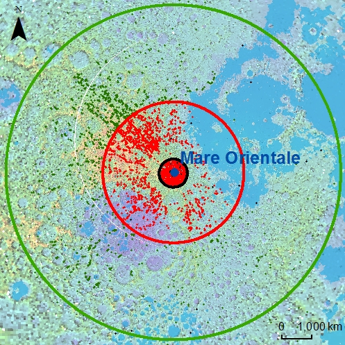
Figure 1.
Sketch map showing the geomorphological setting of the area for machine learning training and testing. Background map is a hillshade image from Lunar Orbiter Laser Altimeter elevation data. Dark blue dots mark the crater and crater basin center with names labeled in dark blue. Black circle depicts the boundary of the Orientale Basin.
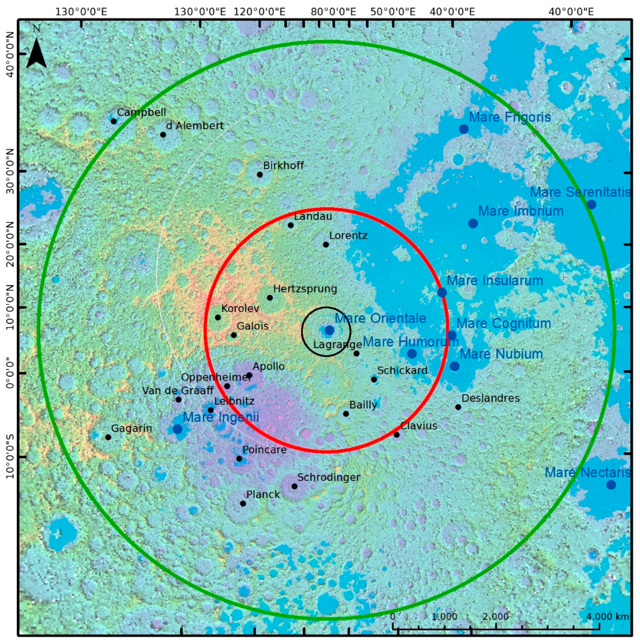
Figure 2.
Sketch map showing samples of different datasets. Red points represent samples in the training dataset, black points show samples in Testing Dataset I, and green points mark samples in Testing Dataset II. Black circle depicts the boundary of the Orientale Basin. Red and green circles denote the region at the center of the basin and extending out to a radial distance of 3.5 radius (R) and 6 R, respectively.
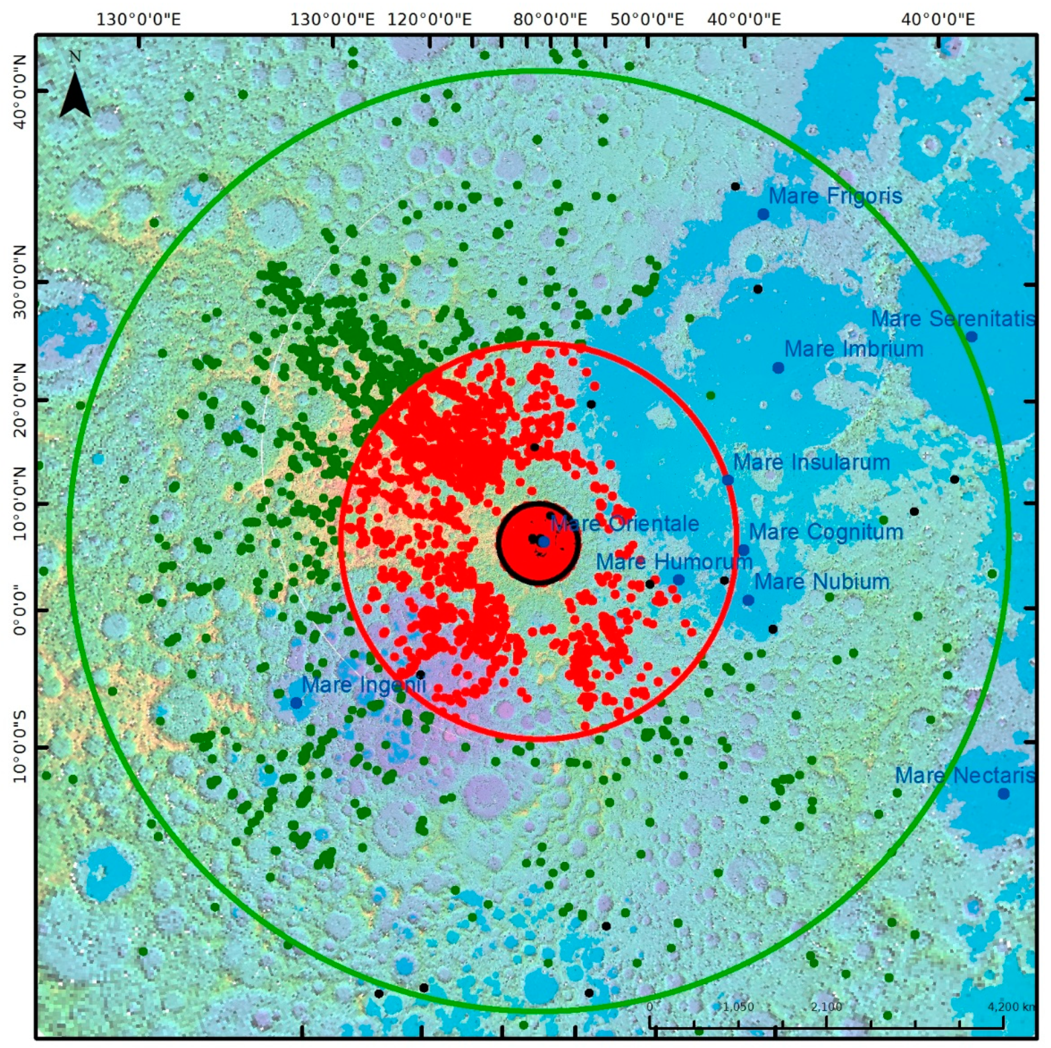
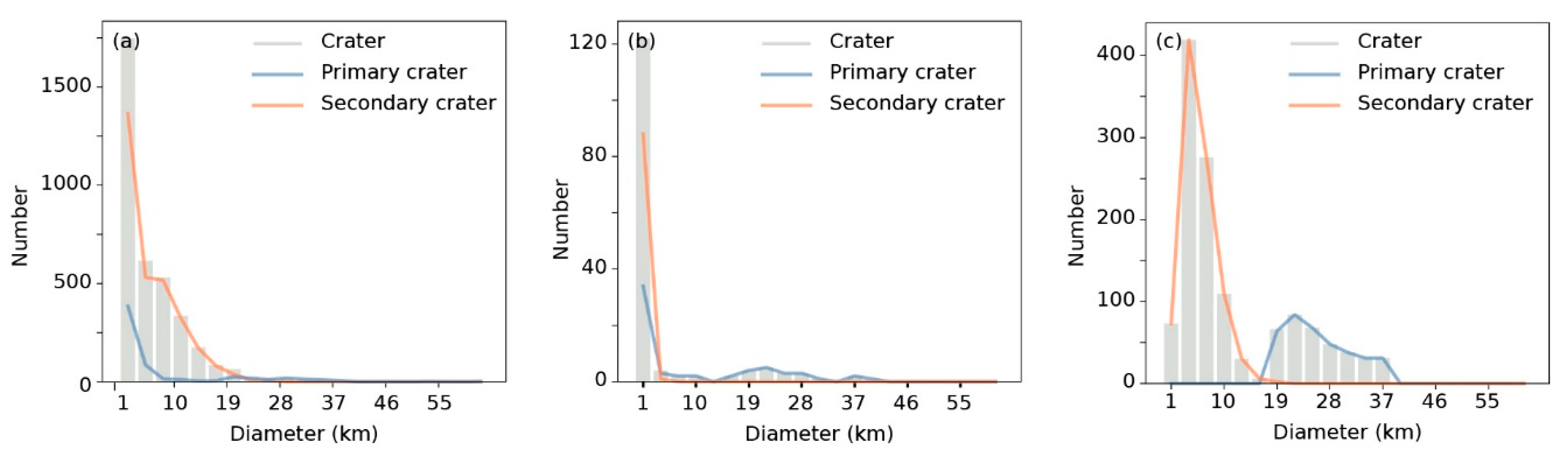
Figure 3.
Diameter distribution of craters in three datasets: (a) training dataset, (b) Testing Dataset I, (c) Testing Dataset II. Geometric scale of bins is the fourth root of 2, and the leftmost edge represents the smallest diameter, 1 km. This figure uses the same geometric scale of bins when involving diameter.
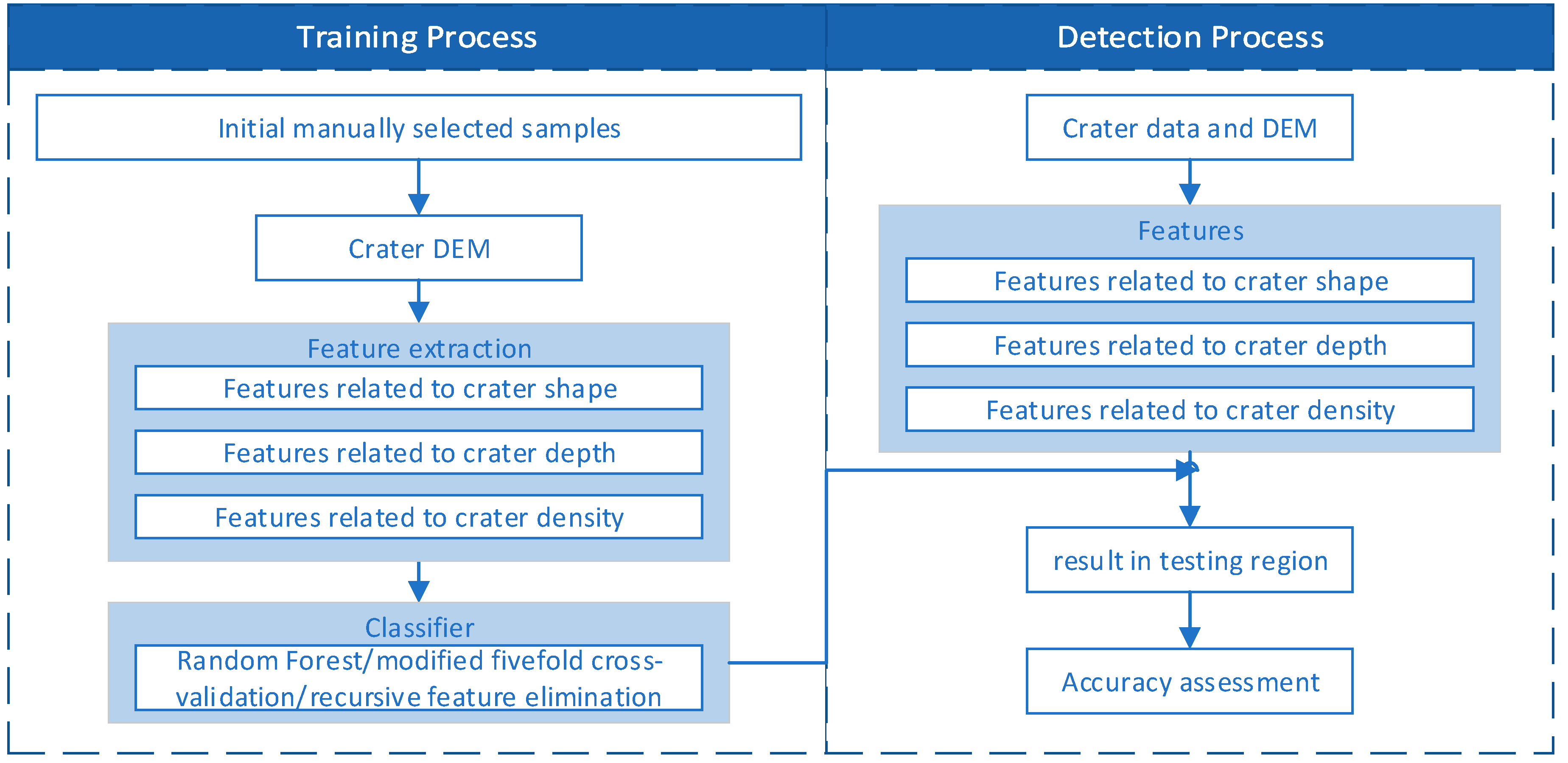
Figure 4.
Workflow of this study. DEM, digital elevation model.
Figure 4.
Workflow of this study. DEM, digital elevation model.
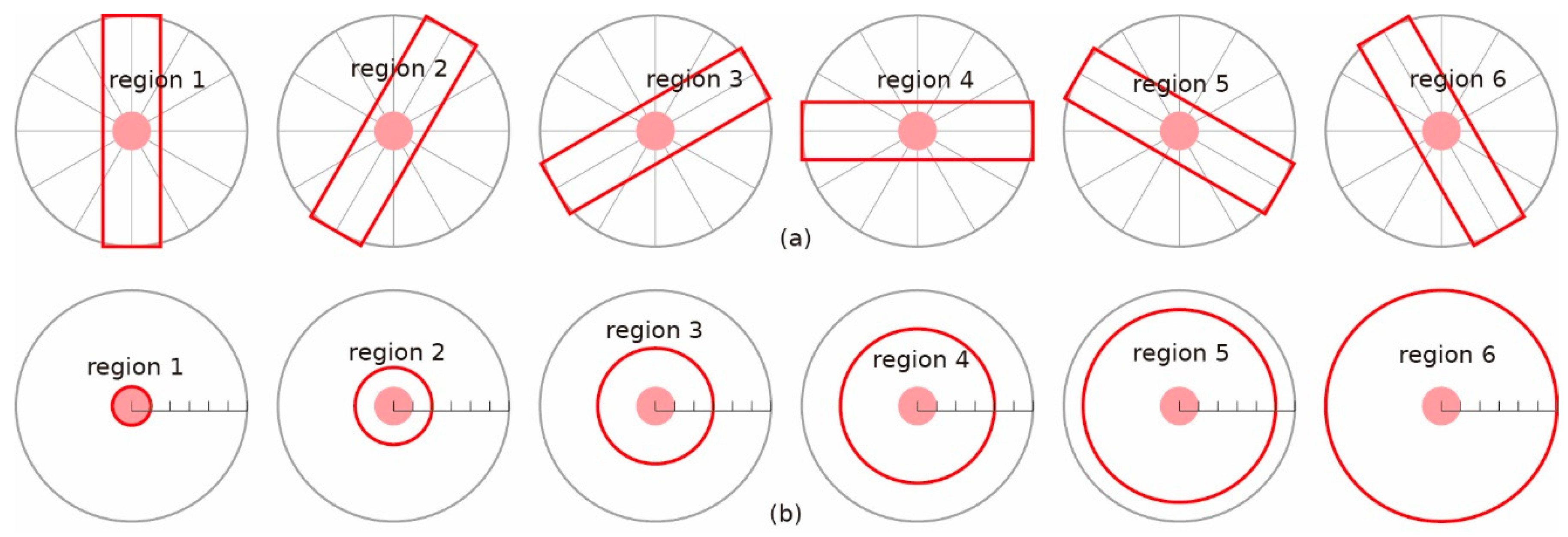
Figure 5.
Sketch maps showing corresponding regions used for calculating features related to crater density related to (a) crater chain and (b) crater cluster. Light red circles represent craters whose features are calculated. Dark red regions labeled 1, 2, 3, 4, 5, 6 mark corresponding regions for calculating , . Gray circles show regions at the centers of craters and extended out to a radial distance of 6 R (R is crater radius).
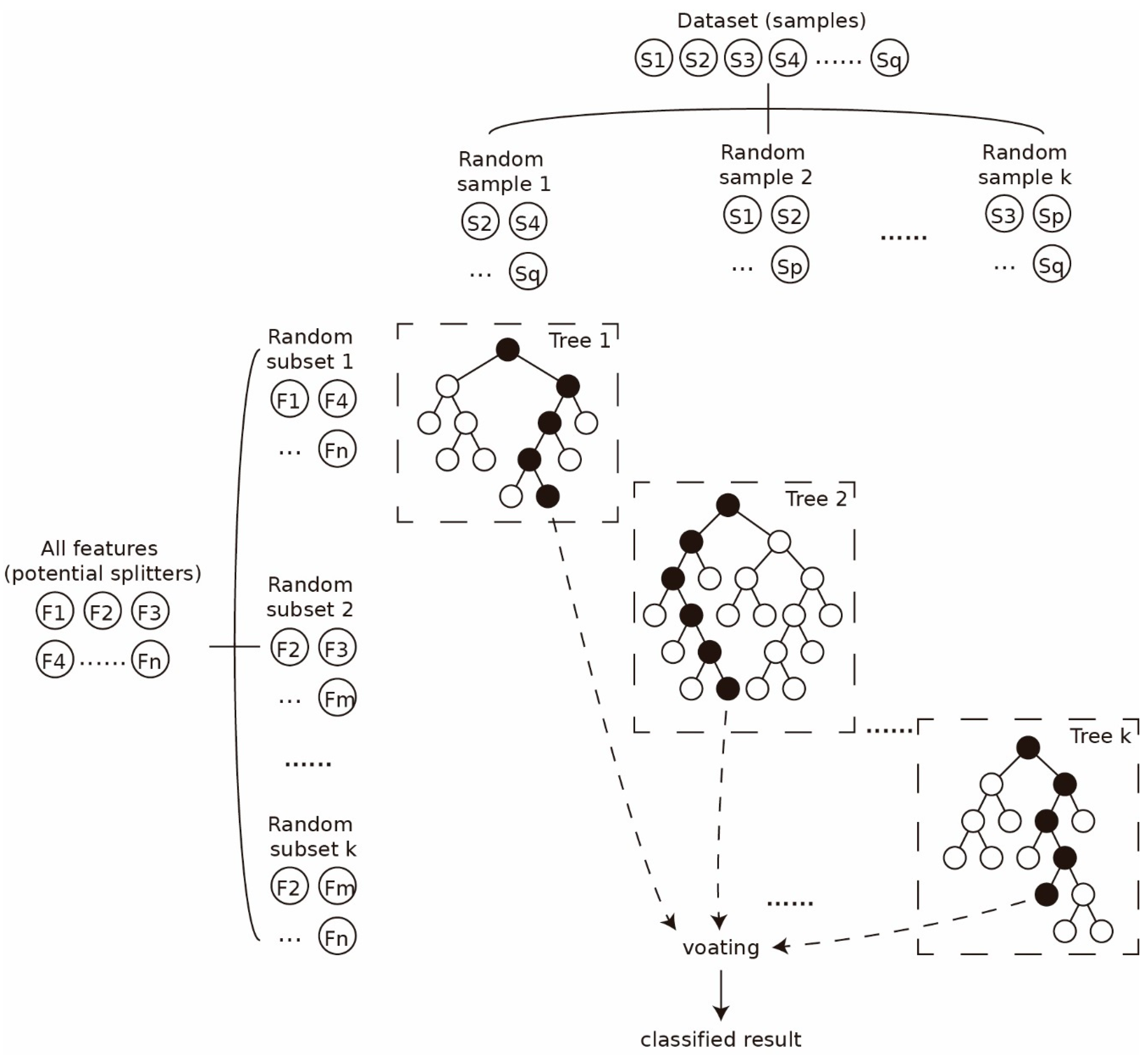
Figure 6.
Sketch map showing a random forest classifier.
Figure 6.
Sketch map showing a random forest classifier.
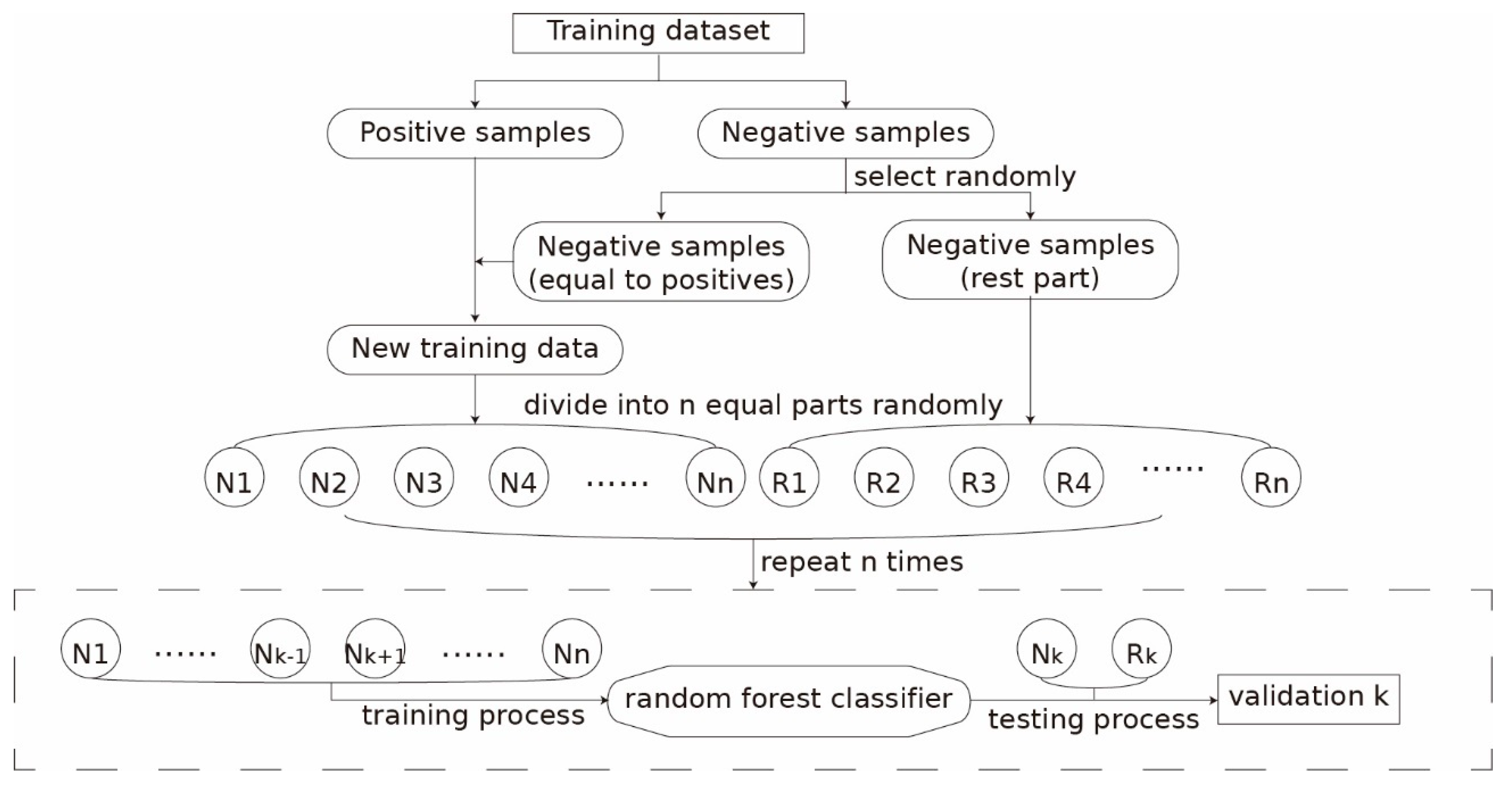
Figure 7.
Sketch map showing a modified nfold cross-validation.
Figure 7.
Sketch map showing a modified nfold cross-validation.
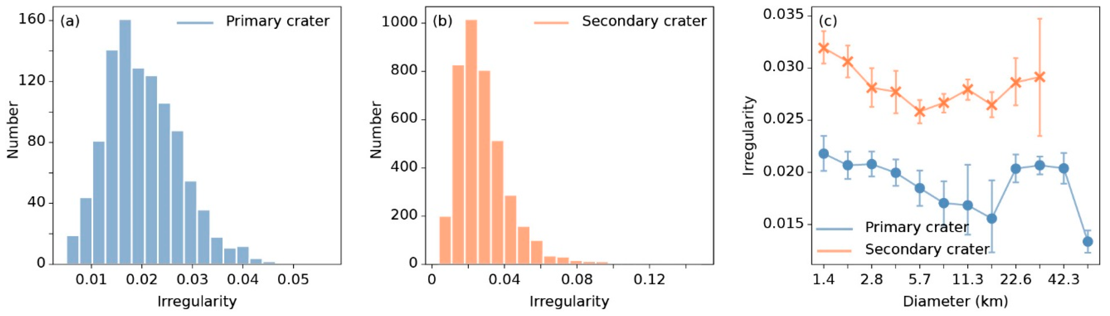
Figure 8.
Histograms of irregularity distribution of (a) primary craters and (b) secondary craters, and (c) the relationship between the statistics irregularity and diameter. In (c), the points represent mean irregularity. Blue lines and points represent primary craters, and orange lines and points represent secondary craters.
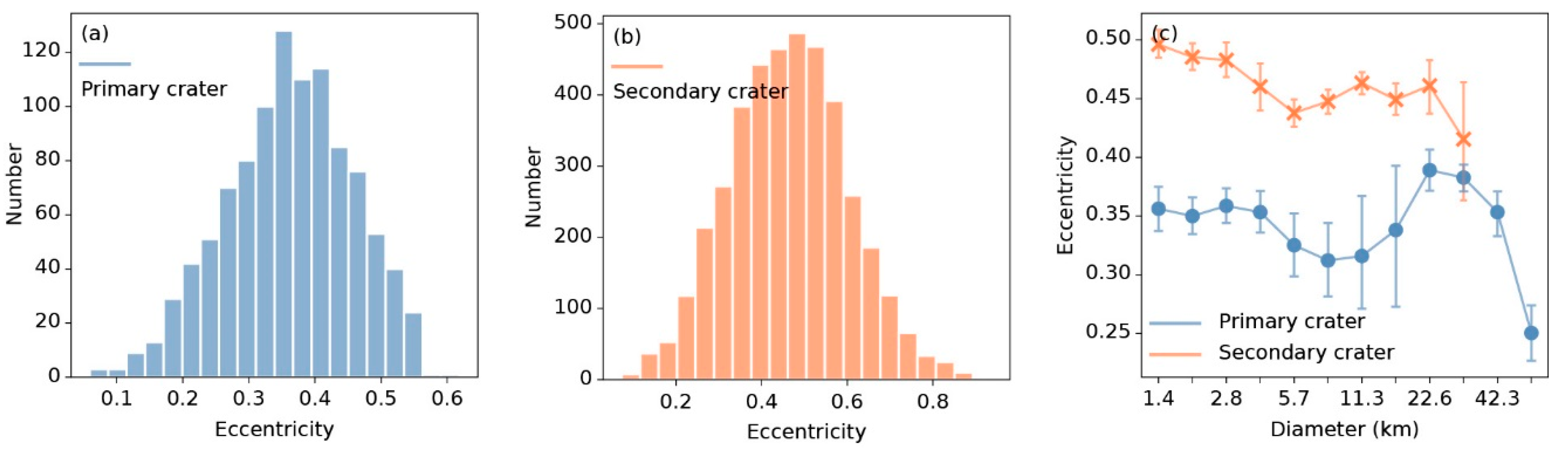
Figure 9.
Histograms of eccentricity distribution of (a) primary craters and (b) secondary craters, and (c) the relationship between the statistics eccentricity and diameter. In (c), points represent mean eccentricity. Blue lines and points represent primary craters, and orange lines and points represent secondary craters.
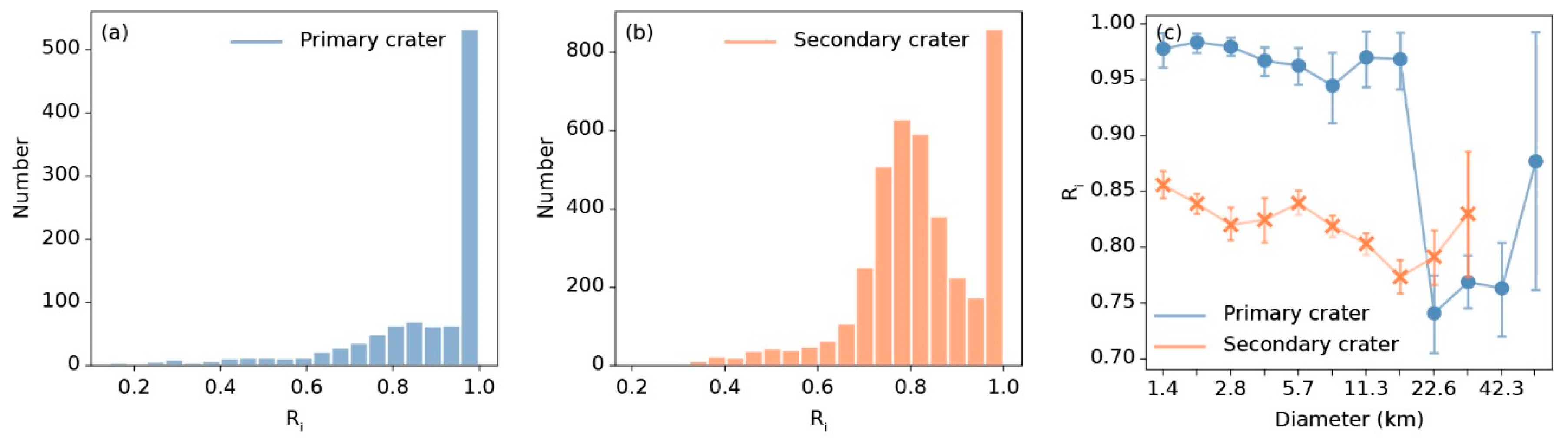
Figure 10.
Histograms of rim integrity distribution of (a) primary craters and (b) secondary craters, and (c) the relationship between the statistics boundary integrity and diameter. In (c), points represent mean rim boundaries. Blue lines and points represent primary craters and orange lines and points represent secondary craters.
Figure 11.
Relationship between diameter and (a) standard deviation of fitted circle height (), (b) standard deviation of fitted ellipse height (), (c) fitted circle’s depth-to-diameter ratio (), (d) difference between fitted circle’s depth-to-diameter ratio () and fitted ellipse depth to major axis (), (e) difference between fitted circle depth-to-diameter ratio () and fitted ellipse depth to minor axis (). Blue lines and points represent primary craters, and orange lines and points represent secondary craters.
Figure 12.
Relationship between diameters and (a) ranges of Chain_I of primary craters, (b) ranges of Chain_I of secondary craters, (c) ranges of Chain_II of primary craters, (d) ranges of Chain_II of secondary craters. Blue boxes represent primary craters and orange boxes represent secondary craters.
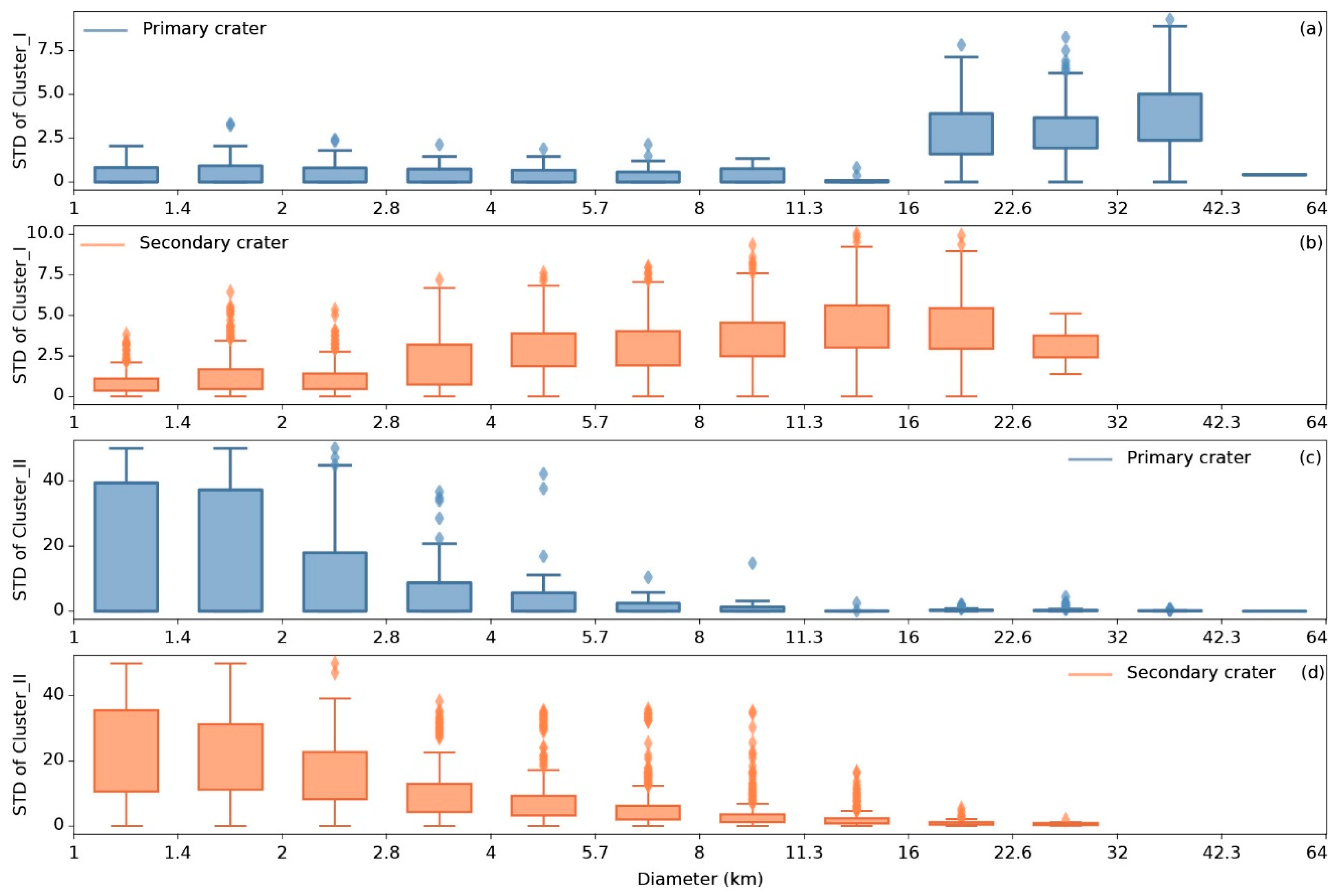
Figure 13.
Relationship between diameter and standard deviation (STD) of (a) 1 for primary craters, (b) for secondary craters, (c) for primary craters, (d) for secondary craters. Blue boxes represent primary craters and orange boxes represent secondary craters.
Figure 13.
Relationship between diameter and standard deviation (STD) of (a) 1 for primary craters, (b) for secondary craters, (c) for primary craters, (d) for secondary craters. Blue boxes represent primary craters and orange boxes represent secondary craters.
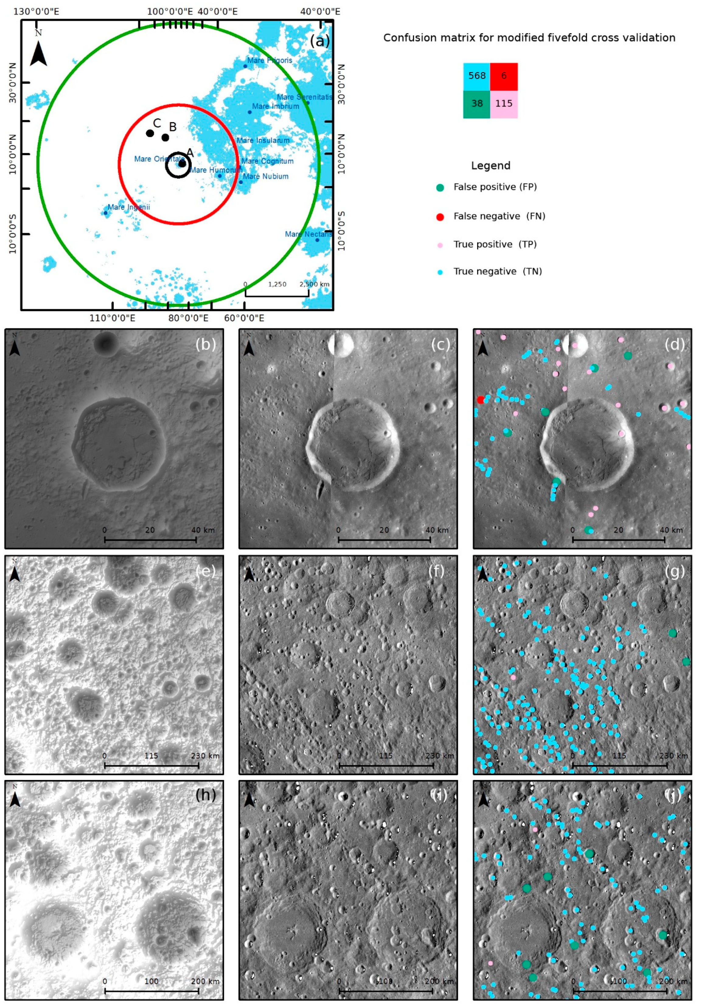
Figure 14.
Fivefold cross-validation results: (a) sketched map showing locations of regions A, B, and C; (b–d) DEM and LROC-WAC (Lunar Reconnaissance Orbiter Camera-wide angle camera) images, and classification results for region A; (e–g) DEM and LROC-WAC images, and classification results for region B; (h–j) DEM and LROC-WAC images, and classification results for region C. Green points represent false positive (FP), red points represent false negative (FN), pink points represent true positive (TP), and blue points represent true negative (TN).
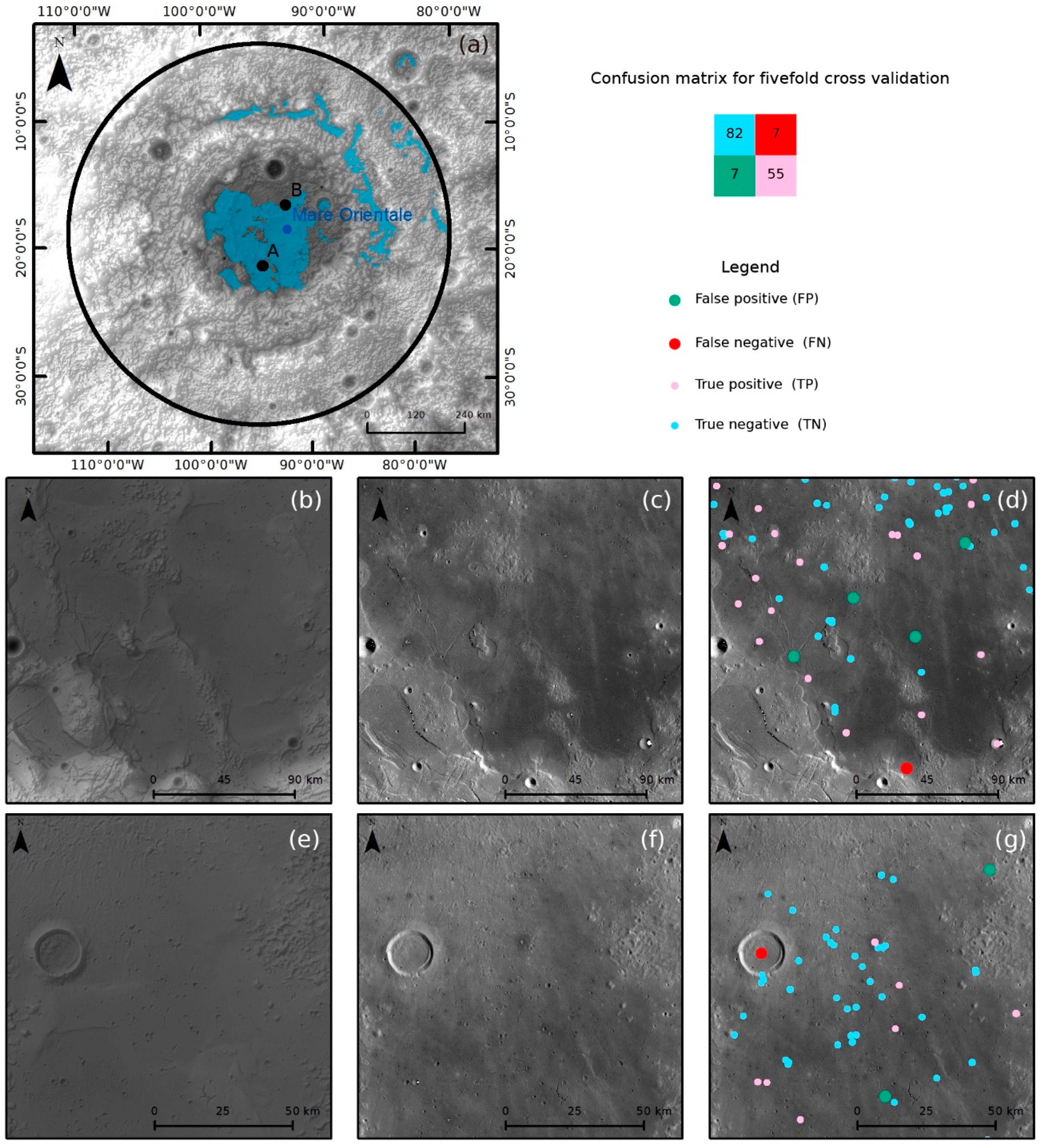
Figure 15.
Testing Dataset I validation results showing classification results by enlarging two regions in dataset I: (a) sketched map showing locations of Regions A and B; (b–d) DEM and LROC-WAC images, and classification results for region A; (e–g) DEM and LROC-WAC images, and classification results for Region B; Green points represent FP, red points represent FN, pink points represent TP, and blue points represent TN.
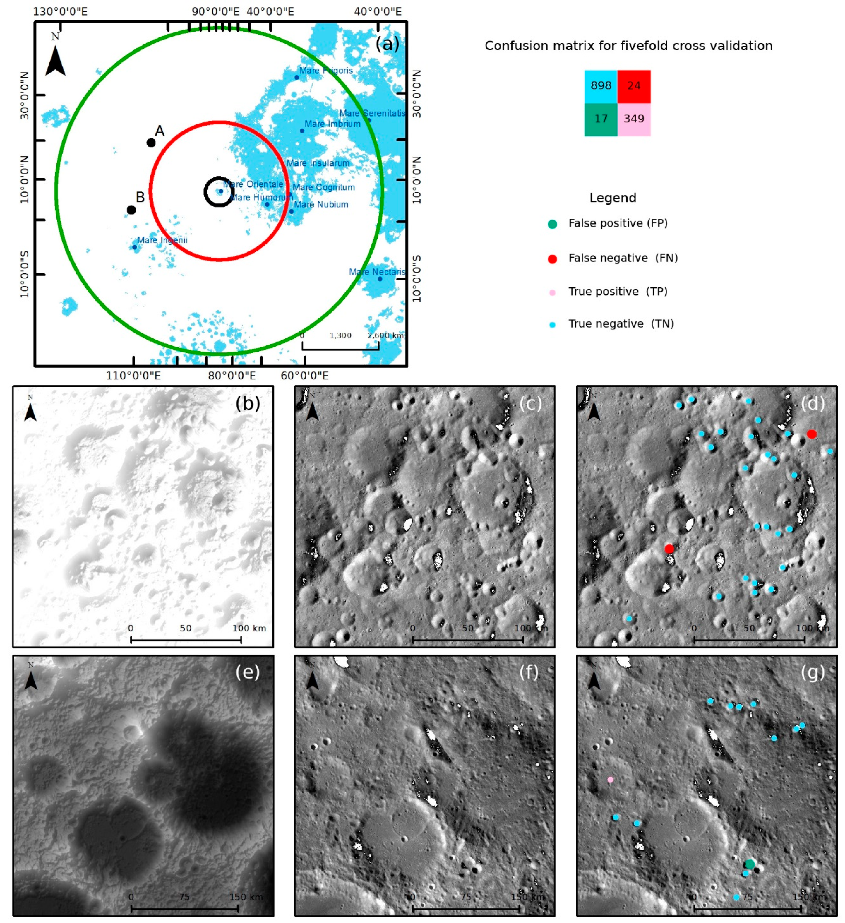
Figure 16.
Testing dataset II validation results: (a) sketched map showing locations of Regions A and B; (b–d) DEM and LROC-WAC images, and classification results for region A; (e–g) DEM and LROC-WAC images, and classification results for Region B. Green points represent FP, red points represent FN, pink points represent TP, and blue points represent TN.
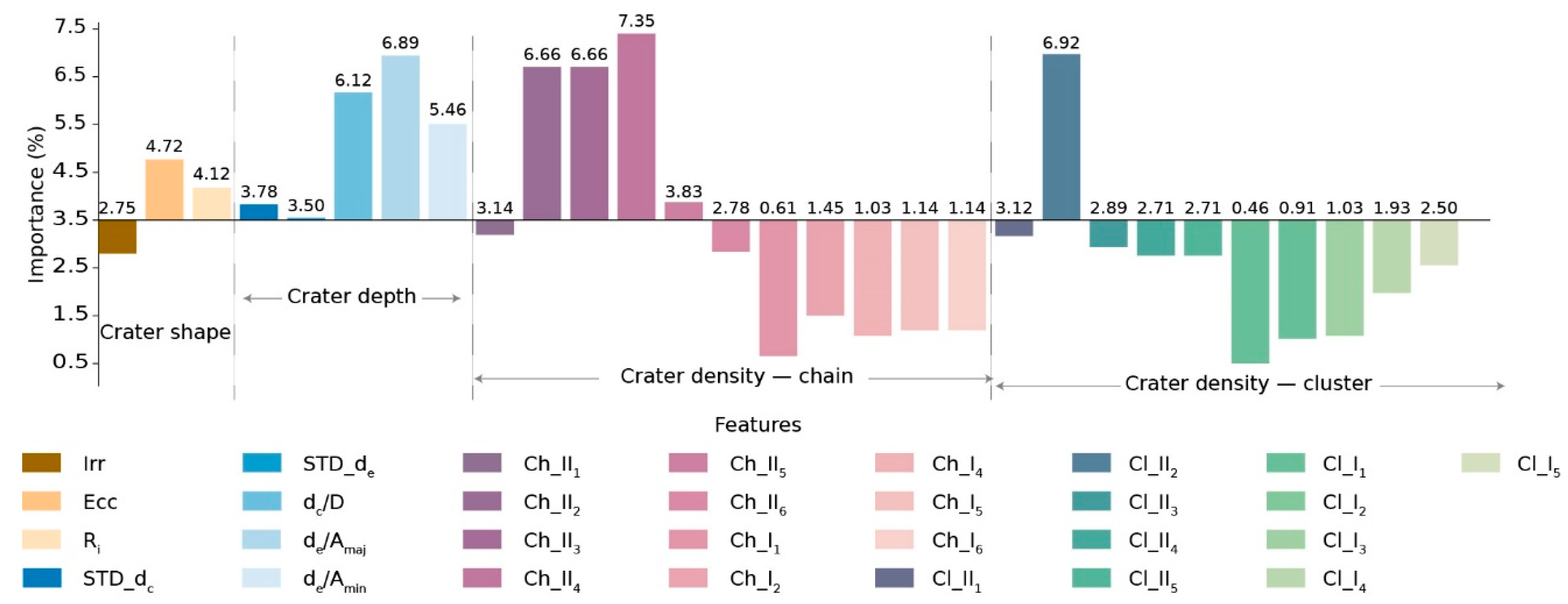
Figure 17.
Relative importance values of features.
Figure 17.
Relative importance values of features.
Table 1.
Statistics of crater inventory.
Table 1.
Statistics of crater inventory.
| Parameter | Value |
|---|
| Primary Craters | Secondary Craters | Craters |
|---|
| Count | 1032 | 4041 | 5073 |
| Mean | 14.77 | 6.25 | 7.98 |
| Standard deviation | 12.93 | 4.55 | 7.89 |
| Minimum | 1.18 | 1.18 | 1.18 |
| 25th percentile | 2.31 | 1.90 | 2.01 |
| Median | 8.50 | 5.66 | 5.72 |
| 75th percentile | 25.80 | 8.94 | 10.08 |
| Maximum | 63.06 | 27.74 | 63.06 |
Table 2.
Classification of crater inventory.
Table 2.
Classification of crater inventory.
| Classification | Training Dataset | Testing Dataset I | Testing Dataset II
2 | Sum |
|---|
| Way 1 | Primary craters | 510 | 44 | 0 | 554 |
| Secondary craters | 1331 | 89 | 0 | 1420 |
| Way II | Primary craters | 0 | 0 | 0 | 0 |
| Secondary craters | 1706 | 0 | 915 | 2621 |
| Way III | Primary craters | 96 | 18 | 364 | 478 |
| Secondary craters | 0 | 0 | 0 | 0 |
| Sum | Primary craters | 606 | 62 | 364 | 1032 |
| Secondary craters | 3037 | 89 | 915 | 4041 |
| Craters | 3643 | 151 | 1279 | 5073 |
Table 3.
Statistics of irregularity.
Table 3.
Statistics of irregularity.
| Parameter | Value |
|---|
| Primary Craters | Secondary Craters | Craters |
|---|
| Count | 1032 | 4041 | 5073 |
| Mean | 0.020 | 0.028 | 0.027 |
| Standard deviation | 0.007 | 0.015 | 0.014 |
| Minimum | 0.005 | 0.004 | 0.004 |
| 25th percentile | 0.015 | 0.018 | 0.017 |
| Median | 0.019 | 0.025 | 0.024 |
| 75th percentile | 0.025 | 0.035 | 0.032 |
| Maximum | 0.057 | 0.148 | 0.148 |
Table 4.
Statistics of eccentricity.
Table 4.
Statistics of eccentricity.
| Parameter | Value |
|---|
| Primary Craters | Secondary Craters | Craters |
|---|
| Count | 1032 | 4041 | 5073 |
| Mean | 0.36 | 0.46 | 0.44 |
| Standard deviation | 0.10 | 0.14 | 0.14 |
| Minimum | 0.06 | 0.07 | 0.06 |
| 25th percentile | 0.30 | 0.37 | 0.35 |
| Median | 0.37 | 0.46 | 0.44 |
| 75th percentile | 0.43 | 0.56 | 0.53 |
| Maximum | 0.62 | 0.94 | 0.94 |
Table 5.
Statistics of boundary integrity.
Table 5.
Statistics of boundary integrity.
| Parameter | Value |
|---|
| Primary Craters | Secondary Craters | Craters |
|---|
| Count | 1032 | 4041 | 5073 |
| Mean | 0.87 | 0.82 | 0.83 |
| Standard deviation | 0.18 | 0.13 | 0.15 |
| Minimum | 0.14 | 0.20 | 0.14 |
| 25th percentile | 0.80 | 0.75 | 0.75 |
| Median | 0.98 | 0.81 | 0.83 |
| 75th percentile | 1.00 | 0.92 | 1.00 |
| Maximum | 1.00 | 1.00 | 1.00 |
Table 6.
Statistics of the range of .
Table 6.
Statistics of the range of .
| Parameter | Value |
|---|
| Primary Craters | Secondary Craters | Craters |
|---|
| Count | 1032 | 4041 | 5073 |
| Mean | 1.18 | 1.84 | 1.71 |
| Standard deviation | 1.24 | 1.33 | 1.34 |
| Minimum | 0.00 | 0.00 | 0.00 |
| 25th percentile | 0.00 | 1.00 | 1.00 |
| Median | 1.00 | 2.00 | 2.00 |
| 75th percentile | 2.00 | 3.00 | 3.00 |
| Maximum | 7.00 | 9.00 | 9.00 |
Table 7.
Statistics of standard deviation for .
Table 7.
Statistics of standard deviation for .
| Parameter | Value |
|---|
| Primary Craters | Secondary Craters | Craters |
|---|
| Count | 1032 | 4041 | 5073 |
| Mean | 1.69 | 2.59 | 2.40 |
| Standard deviation | 1.72 | 1.86 | 1.87 |
| Minimum | 0.00 | 0.00 | 0.00 |
| 25th percentile | 0.37 | 1.00 | 0.76 |
| Median | 1.07 | 2.34 | 2.11 |
| 75th percentile | 2.63 | 3.80 | 3.64 |
| Maximum | 9.29 | 10.02 | 10.02 |
Table 8.
Statistics of model performance.
Table 8.
Statistics of model performance.
| Precision | Sensitivity | Accuracy | F1-score | Kappa |
|---|
| Training dataset | 1 | 1 | 1 | 1 | 1 |
| Testing dataset | 0.752 | 0.950 | 0.939 | 0.839 | 0.803 |
Table 9.
Statistics of Testing Dataset I.
Table 9.
Statistics of Testing Dataset I.
| Precision | Sensitivity | Accuracy | F1-score | Kappa |
|---|
| Testing Dataset I | 0.887 | 0.887 | 0.907 | 0.887 | 0.808 |
Table 10.
Statistics of Testing Dataset II.
Table 10.
Statistics of Testing Dataset II.
| Precision | Sensitivity | Accuracy | F1-score | Kappa |
|---|
| Testing dataset II | 0.952 | 0.934 | 0.968 | 0.943 | 0.921 |

 ,
, 


