A Decentralized Processing Schema for Efficient and Robust Real-time Multi-GNSS Satellite Clock Estimation

Abstract

Real-time multi-GNSS precise point positioning (PPP) requires the support of high-rate satellite clock corrections. Due to the large number of ambiguity parameters, it is difficult to update clocks at high frequency in real-time for a large reference network. With the increasing number of satellites of multi-GNSS constellations and the number of stations, real-time high-rate clock estimation becomes a big challenge. In this contribution, we propose a decentralized clock estimation (DECE) strategy, in which both undifferenced (UD) and epoch-differenced (ED) mode are implemented but run separately in different computers, and their output clocks are combined in another process to generate a unique product. While redundant UD and/or ED processing lines can be run in offsite computers to improve the robustness, processing lines for different networks can also be included to improve the clock quality. The new strategy is realized based on the Position and Navigation Data Analyst (PANDA) software package and is experimentally validated with about 110 real-time stations for clock estimation by comparison of the estimated clocks and the PPP performance applying estimated clocks. The results of the real-time PPP experiment using 12 global stations show that with the greatly improved computational efficiency, 3.14 cm in horizontal and 5.51 cm in vertical can be achieved using the estimated DECE clock.

1. Introduction

As one of the most popular positioning technologies, precise point positioning (PPP) [1,2] has been widely used thanks to its high accuracy, proficiency, stability, and flexibility [3,4,5]. Recently, with the great progress of global navigation satellite systems (GNSS), the Russian GLONASS, European Galileo, and Chinese BeiDou have increased the number of satellites to more than 80, which will grow to about 120 in 2020. Compared with GPS-only solutions, better performance of PPP with multi-GNSS would be achieved in terms of not only convergence but also accuracy because of the improved satellite geometry due to the increasing number of satellites [6,7,8,9,10]. With the progress in high-speed internet communication and the achievements in the GNSS data stream protocol and format design, i.e., Radio Technical Commission for Maritime (RTCM) and Networked Transport of RTCM via Internet Protocol (NTRIP) [11], great efforts are underway towards the global real-time GNSS precise positioning service, where the real-time high precision satellite orbit and clock product is fundamental [12]. Though the quality of the International GPS Service (IGS) precise clock products have been improved continually since 1994 [13], to provide real-time satellite clocks of high resolution, normally to be updated within five seconds, is still full of challenges. Moreover, the heavy computational burden against the requirement on high update rate and involvement of more stations and multi-constellation satellites is one of the crucial issues.

In the typical clock estimation, undifferenced (UD) observations are employed and the computation time depends mainly on the number of estimated ambiguity parameters [14]. Obviously the computation becomes much more time-consuming if more stations are involved for reliable estimation. The task, to update clocks within five seconds, could be fulfilled with difficulty for multi-GNSS clock estimation, with about 80 satellites now and about 120 satellites soon. Furthermore, for such a large linear system, a sophisticated quality control procedure, which must be implemented, also needs significant computation time.

Bock et al. employed epoch-differenced (ED) phase observations to densify CODE’s final clock of 5-min intervals to 1 Hz for special precise applications, in which the 5-min clocks derived by using undifferenced (UD) phase and range observations are fixed as “control points” [15]. Generally, UD provides absolute clocks, while ED generates the high-rate clock change as the majority of parameters, e.g., ambiguities are eliminated and consequently the computation load is significantly reduced. On the same basis, Zhang and Li extended this method for real-time clock estimation with a dual-thread strategy; the UD thread is for the absolute clock estimation with an interval of five seconds, while the ED thread estimates the clock change with an interval of one second [16]. The ED clocks are aligned to the UD ones to generate the final high-rate satellite clocks to meet the requirements of real-time kinematic PPP.

Furthermore, Ge et al. introduced an alternative approach to estimate high-rate real-time satellite clocks using ED phase and UD range observations in a single filter, so that no ambiguities are estimated and clock changes are aligned by range to absolute clocks [17]. The result shows that the approach can achieve a comparable accuracy to that of the UD approach, whereas the computation time is reduced to one tenth. This strategy was also implemented into real-time multi-GNSS clock estimation and evaluated [18,19,20].

At the same time, fast computation approaches optimized according to CPU structure, such as matrix operations, were also skillfully introduced into GNSS data processing in order to improve the computational efficiency [21]. Ambiguity resolution was also implemented to reduce the number of active ambiguities, and consequently, the computation burden for clock estimation [22,23].

Anyway, as discussed above, the mixed-differenced method with UD for absolute clocks and ED for clock variation is one of the most efficient strategies for multi-GNSS clock estimation with large networks, although UD is now widely used. One of the remaining issues is how to combine the UD and ED, integrated into one process as parallel inline processes [16] or even in a single adjustment [17]. Although the theoretical difference is slight, the reliability and robustness of the processing schema are of great concern for providing satellite clocks for real-time operational service. For this purpose, we have to consider the following two aspects. First of all, redundant processing lines are definitely needed and can be deployed either in the same location or offsite, and their outputs can be combined to a unique product for providing reliable service. It will not affect the performance if some of the redundant processing lines are crashed. Second, disturbed processing may be needed if a network cannot be processed in a single adjustment because of too many stations and/or satellites. In fact, along with the development of modern processors and servers, the parallel computing on a distributed framework is receiving increasing interest in scientific computation community.

In this contribution, we develop an alternative processing strategy for multi-GNSS real-time high-rate clock estimation, in which a number of UD and ED processing lines can be involved and their output clocks are combined to generate a unique clock product. The UD and EU lines can be designed for sub-networks or a set of GNSS systems, or duplicated lines for redundancy. They can be deployed and operated independently over different and even offsite computers. Then, the ED and UD clocks are combined with separated software developed by us in a similar way to that done for the combination of analysis center (AC) products at the IGS real-time combination center [24]. As each of the processing lines can be run in different computers, we named it decentralized clock estimation (DECE) in this study.

The processing strategy is realized based on the Position and Navigation Data Analyst (PANDA) software for validation [25,26]. A network of about 110 real-time stations with the tracking capacity of GPS, GLONASS, Galileo, and BeiDou four systems is employed and real-time estimated clocks, as well as the computation time using the UD processing mode and the DECE mode, are compared and the PPP performance is also evaluated.

First, we introduce the current research status for multi-GNSS and real-time clock estimation, and then the multi-GNSS real-time clock estimation model is discussed. In addition, we present the strategy of data processing and the real-time clock estimation system based on PANDA software. The real-time clock product estimated by the DECE strategy is also validated by clock comparison and their application to multi-GNSS PPP. Finally, a summary of the results and corresponding conclusions are given.

2. Multi-GNSS (Global Navigation Satellite Systems) Clock Estimation

As UD and ED observations are the basic observations used in most of the current clock estimation as well as in this study, the corresponding observation equations for multi-GNSS clock estimation will be introduced and discussed in this section followed by the process for clock combination.

2.1. Undifferenced Observation Model

In the clock estimation using UD observations, both carrier phase and pseudorange observations are involved, and the ionospheric-free linear combination is formulated to eliminate the first-order ionospheric delay. Thus, the UD observation model for a given epoch is expressed as

$$\{\begin{array}{l}{v}_{LC}^G=d{t}_r-d{T}_{}^{s,G}+b_{r,LC}^G-b_{LC}^{s,G}+m\cdot d_{trop}^{}+N_{}^G+l_{LC}^G\\ v_{PC}^G=d{t}_r-d{T}_{}^{s,G}+b_{r,PC}^G-b_{PC}^{s,G}+m\cdot d_{trop}^{}+l_{PC}^G\\ v_{LC}^R=d{t}_r-d{T}_{}^{s,R}+b_{r,LC}^R-b_{LC}^{s,R}+m\cdot d_{trop}^{}+N_{}^R+l_{LC}^R\\ v_{PC}^R=d{t}_r-d{T}_{}^{s,R}+b_{r,PC}^R-b_{PC}^{s,R}+m\cdot d_{trop}^{}+l_{PC}^R\\ v_{LC}^E=d{t}_r-d{T}_{}^{s,E}+b_{r,LC}^E-b_{LC}^{s,E}+m\cdot d_{trop}^{}+N_{}^E+l_{LC}^E\\ v_{PC}^E=d{t}_r-d{T}_{}^{s,E}+b_{r,PC}^E-b_{PC}^{s,E}+m\cdot d_{trop}^{}+l_{PC}^E\\ v_{LC}^C=d{t}_r-d{T}_{}^{s,C}+b_{r,LC}^C-b_{LC}^{s,C}+m\cdot d_{trop}^{}+N_{}^C+l_{LC}^C\\ v_{PC}^C=d{t}_r-d{T}_{}^{s,C}+b_{r,PC}^C-b_{PC}^{s,C}+m\cdot d_{trop}^{}+l_{PC}^C\end{array},$$

(1)

where $s$, $r$ are subscript for the satellite and receiver, and the subscript $G$, $R$, $E$, $C$ represent GPS, GLONASS, Galileo, and BeiDou satellite, respectively; $PC$ and LC denote ionospheric-free pseudorange and phase observations, respectively; $d{t}_r$ and $d{T}^s$ are receiver and satellite clock corrections, respectively; $b_r$ and $b^s$ are the signal delay bias in receiver and satellite, respectively; $d_{trop}$ represents the zenith tropospheric delay while m is the corresponding mapping coefficient; $N$ denotes the ambiguity of the ionosphere-free phase observations. $v$ and $l$ are the post-fit residuals pre-fit residuals of the ionospheric-free observations, respectively. In addition, the antenna phase center corrections, the phase windup, as well as the code bias between different types of codes, e.g., differential code biases (DCB) of P1 and C1, should be considered in Equation (1).

Concerning the satellite DCB, which is stable enough as demonstrated by Dach et al. [27], it can normally be absorbed by clock corrections in the data processing. In other words, the final clock estimation is a combination of the “true” clock and satellite DCB. In addition, since the initial information in normal equation is mostly provided by pseudorange observation and GPS time is usually chosen as the time reference, an additional Inter-System Bias (ISB) parameter can be introduced for R, E, and C to compensate its offset from GPS. The Inter-Frequency phase Bias (IFB) of GLONASS signals are estimated in the orbit determination and corrected as a constant in clock estimation. Thus, Equation (1) can be expressed as

$$\{\begin{array}{l}{v}_{LC}^G=d{t}_r-d{\tilde{T}}_{}^{s,G}+m\cdot d_{trop}^{}+N_{}^G+l_{LC}^G\\ v_{PC}^G=d{t}_r-d{\tilde{T}}_{}^{s,G}+m\cdot d_{trop}^{}+l_{PC}^G\\ v_{LC}^R=d{t}_r+IS{B}_{}^R-d{\tilde{T}}_{}^{s,R}+m\cdot d_{trop}^{}+N_{}^R+l_{LC}^R\\ v_{PC}^R=d{t}_r+IS{B}_{}^R-d{\tilde{T}}_{}^{s,R}+m\cdot d_{trop}^{}+l_{PC}^R\\ v_{LC}^E=d{t}_r+IS{B}_{}^E-d{\tilde{T}}_{}^{s,E}+m\cdot d_{trop}^{}+N_{}^E+l_{LC}^E\\ v_{PC}^E=d{t}_r+IS{B}_{}^E-d{\tilde{T}}_{}^{s,E}+m\cdot d_{trop}^{}+l_{PC}^E\\ v_{LC}^C=d{t}_r+IS{B}_{}^C-d{\tilde{T}}_{}^{s,C}+m\cdot d_{trop}^{}+N_{}^C+l_{LC}^C\\ v_{PC}^C=d{t}_r+IS{B}_{}^C-d{\tilde{T}}_{}^{s,C}+m\cdot d_{trop}^{}+l_{PC}^C\end{array},$$

(2)

where $IS{B}^R$, $IS{B}^E$, and $IS{B}^C$ represent the Inter-System Bias of GLONASS, Galileo, and BeiDou, relative to GPS, and $d{\tilde{T}}^s$ is the satellite clock absorbing the satellite-related code bias.

Due to the fact that the receiver clock terms are linearly dependent with the satellite clock, any bias in the receiver clock estimate can be compensated by the satellite clock estimates. In addition, since an individual receiver clock parameter for each satellite system is estimated, the datum deficiency exists for each system. Thus, the following constraint is introduced for each satellite system [14]:

$$\{\begin{array}{c}{\displaystyle \sum _{s}d{\tilde{T}}^{s,G}=0}\\ {\displaystyle \sum _{s}d{\tilde{T}}^{s,R}=0}\\ {\displaystyle \sum _{s}d{\tilde{T}}^{s,E}=0}\\ {\displaystyle \sum _{s}d{\tilde{T}}^{s,C}=0}\end{array},$$

(3)

As presented in Equation (3), the sum of the satellite clock error for each system is set as zero to separate the receiver clock and the corresponding satellite clock.

In the solution of the satellite clock based on Equations (2) and (3), all parameters listed in

Table 1. Parameters need to be estimated at each epoch in the undifferenced (UD) model.

Item	Parameters Number
Receiver clock and Inter-System Bias (ISB)	$n_{sys}\times n_{site}$
Satellite clock corrections	$n_{sat}$
Zenith troposphere delay	$n_{site}$
Undifferenced ambiguity	$n_{sys}\times n_p\times n_{site}$
Total $n_{tot}$	$(n_{sys}+1+n_{sys}\times n_p)\times n_{site}+n_{sat}$

are going to be estimated simultaneously. Suppose that $n_{sys}$, $n_{site}$, and $n_{sat}$ are the numbers of navigation systems, stations, and total multi-GNSS satellites, respectively, while the averaged satellite number that is tracked at each station each epoch for a single system is $n_p$. Thus, the parameters to be estimated with Equation (2) are listed in Table 1.

Assuming the numbers of satellites for GPS, GLONASS, Galileo, and BeiDou are 32, 27, 30, and 35, respectively. Without loss of generality, it is assumed that $n_p=8$, while for the GPS-only solution, $n_{sys}=1$, $n_{sat}=32$, and thus the total number of parameters at each epoch is $n_{tot}=10\times n_{site}+32$, in the case of a four system multi-GNSS solution, $n_{sys}=4$, $n_{sat}=32+27+30+35=124$, and $n_{tot}=37\times n_{site}+n_{sat}$.

2.2. Epoch-Differenced Model

As is well known, the majority of parameters in the UD model are ambiguities which are increasing linearly with the number of satellites and stations. It is clearly the main reason for the heavy computational burden in the UD model. The motivation of ED model is to eliminate the ambiguity parameters, and consequently reduce the computation load. The ED observation equations at each epoch can be expressed as follows,

$$\{\begin{array}{l}\Delta v_{LC}^G=\Delta d{t}_r-\Delta d{\tilde{T}}_{}^{s,G}+\Delta m\cdot d_{trop}^{}+\Delta l_{LC}^G\\ \Delta v_{PC}^G=\Delta d{t}_r-\Delta d{\tilde{T}}_{}^{s,G}+\Delta m\cdot d_{trop}^{}+\Delta l_{PC}^G\\ \Delta v_{LC}^R=\Delta d{t}_r+\Delta IS{B}_{}^R-\Delta d{\tilde{T}}_{}^{s,R}+\Delta m\cdot d_{trop}^{}+\Delta l_{LC}^R\\ \Delta v_{PC}^R=\Delta d{t}_r+\Delta IS{B}_{}^R-\Delta d{\tilde{T}}_{}^{s,R}+\Delta m\cdot d_{trop}^{}+\Delta l_{PC}^R\\ \Delta v_{LC}^E=\Delta d{t}_r+\Delta IS{B}_{}^E-\Delta d{\tilde{T}}_{}^{s,E}+\Delta m\cdot d_{trop}^{}+\Delta l_{LC}^E\\ \Delta v_{PC}^E=\Delta d{t}_r+\Delta IS{B}_{}^E-\Delta d{\tilde{T}}_{}^{s,E}+\Delta m\cdot d_{trop}^{}+\Delta l_{PC}^E\\ \Delta v_{LC}^C=\Delta d{t}_r+\Delta IS{B}_{}^C-\Delta d{\tilde{T}}_{}^{s,C}+\Delta m\cdot d_{trop}^{}+\Delta l_{LC}^C\\ \Delta v_{PC}^C=\Delta d{t}_r+\Delta IS{B}_{}^C-\Delta d{\tilde{T}}_{}^{s,C}+\Delta m\cdot d_{trop}^{}+\Delta l_{PC}^C\end{array},$$

(4)

where $\Delta$ is the difference operator between two adjacent epochs and the meanings of the other parameters are the same as in the UD model. Since the ambiguity parameters are removed, there are only three types of parameters left in the equation and they have been shown in

Table 2. Parameters to be estimated at each epoch in the epoch-differenced (ED) model.

Item	Parameters Number
Receiver clocks	$n_{site}$
Satellite clocks	$n_{sat}$
Zenith troposphere delay	$n_{site}$
Total $n_{tot}$	$2\times n_{site}+n_{sat}$

. Since the code bias between GPS and other systems are stable over a day (Zhang et al., 2016), the $\Delta ISB$ can be neglected in Equation (4). The equations can be expressed as,

$$\{\begin{array}{l}\Delta v_{LC}^G=\Delta d{t}_r-\Delta d{\tilde{T}}_{}^{s,G}+\Delta m\cdot d_{trop}^{}+\Delta l_{LC}^G\\ \Delta v_{PC}^G=\Delta d{t}_r-\Delta d{\tilde{T}}_{}^{s,G}+\Delta m\cdot d_{trop}^{}+\Delta l_{PC}^G\\ \Delta v_{LC}^R=\Delta d{t}_r-\Delta d{\tilde{T}}_{}^{s,R}+\Delta m\cdot d_{trop}^{}+\Delta l_{LC}^R\\ \Delta v_{PC}^R=\Delta d{t}_r-\Delta d{\tilde{T}}_{}^{s,R}+\Delta m\cdot d_{trop}^{}+\Delta l_{PC}^R\\ \Delta v_{LC}^E=\Delta d{t}_r-\Delta d{\tilde{T}}_{}^{s,E}+\Delta m\cdot d_{trop}^{}+\Delta l_{LC}^E\\ \Delta v_{PC}^E=\Delta d{t}_r-\Delta d{\tilde{T}}_{}^{s,E}+\Delta m\cdot d_{trop}^{}+\Delta l_{PC}^E\\ \Delta v_{LC}^C=\Delta d{t}_r-\Delta d{\tilde{T}}_{}^{s,C}+\Delta m\cdot d_{trop}^{}+\Delta l_{LC}^C\\ \Delta v_{PC}^C=\Delta d{t}_r-\Delta d{\tilde{T}}_{}^{s,C}+\Delta m\cdot d_{trop}^{}+\Delta l_{PC}^C\end{array},$$

(5)

All parameters left in the equation are shown in Table 2. It should be noted that the ED zenith troposphere delays cannot be ignored although they are very small, because they have a systematic trend along with time and will bias the estimates if ignored [15,17].

Under the same assumption of the number of satellites for each system above, the total number of unknowns is $2\times n_{site}+32$ and $2\times n_{site}+124$ for GPS-only and multi-GNSS solutions, respectively. However, it is suggested by Equation (5) that only the variation of the clock parameter between epochs, i.e., $\Delta t$, can be estimated in the ED model.

To get an intuitive impression on the comparison of the number of unknowns, Figure 1 illustrates the varying total number of parameters along with the number of stations $n_{sta}$. Let us take $n_{sta}=100$ as an example, the total number of unknowns is 232, 324, 1032, 3824 for ED of GPS-only, ED of multi-GNSS, UD of GPS-only, and UD of multi-GNSS, respectively. It is concluded that the inclusion of the new satellite systems implies a significant increase in computation load for the UD model, whereas this dilemma can be mitigated by using the ED model.

2.3. Clock Combination

Although the ED model is computationally efficient enough to support a high-rate update, it can only provide epoch-differenced clocks. Therefore, the UD model must be involved in order to obtain the absolute clock. Thus, a combination process is essential to generate the final clock product that takes advantage of both ED and UD clocks. Theoretically, we can also consider the combination of several ED and/or UD clock products, such as UD clocks from different software packages or different networks, etc. However, for clarification in the following study, we concentrated on the combination of a single UD and ED products. A simple but efficient approach was implemented by using the latest available UD clocks to align the high-rate clock changes estimated by the ED model to generate the final high-rate absolute clocks.

Assuming that the update interval of the UD model is k times of the ED model, for example, if the update rate of the UD is 20 s and that of ED 5 s, then k = 4, and the combination for post-processing can be expressed as follows [16],

$$dT(t_i)=\{\begin{array}{ll}d{T}_{UD}^{}(t_i)& ,\mathrm{mod}(i,k)=0\\ dT(t_{i-1})+d{T}_{ED}^{}(t_i,t_{i-1})& ,otherwise,i\ge 1\end{array},$$

(6)

where $d{T}_{UD}$, $d{T}_{ED}$ represent the UD and ED clock at each epoch, $dT$ represents the combined clock, t is the epoch time, and the symbol mod means remainder operator. From Equation (6), it can be seen that the essence of this approach is using the last UD estimate to calibrate the ED estimates at the following epochs.

However, in the case of real-time clock estimation, the approach must be adapted, as the computation of the UD model usually takes a much longer time than the ED model. Thus, only the latest available UD clocks could be used to calibrate the ED clocks to absolute ones.

For real-time processing, the update rate of the UD and ED model should be properly selected, i.e., the processing/update interval must be larger than the processing time needed and it must be k times the ED interval. The processing schema is illustrated in Figure 2. In the Figure, j is the epoch index of UD processing, the related epoch time is $t_{j\times k}$, and within two adjacent UD epochs, there are k ED epochs.

According to the above criteria for selecting k, we can assume that at each ED epoch within $t_{j\times k}$ and $t_{(j+1)\times k}$, let us say epoch $t_{j\times k+m}$, the UD clock at epoch $t_{(j-1)\times k}$ is always available, and that at epoch $t_{j\times k}$ it may be available depending on the computation efficiency of the UD process. Thus, the combined clock reads as the first expression of Equation (7) if $d{T}_{UD}^{}(t_{j·k})$ is unavailable at epoch $t_{j\times k}$ while reads as the second expression of Equation (7) if $d{T}_{UD}^{}(t_{j·k})$ is available.

$$dT(t_{j·k+m})=\{\begin{array}{l}d{T}_{UD}^{}(t_{(j-1)·k})+{\displaystyle \sum _{l=(j-1)\times k+1}^{j\times k+m}d{T}_{ED}^{}(t_l,t_{l-1})}\\ d{T}_{UD}^{}(t_{j·k})+{\displaystyle \sum _{l=j\times k+1}^{j\times k+m}d{T}_{ED}^{}(t_l,t_{l-1})}\end{array},$$

(7)

With the following definition,

$$\Delta T_{ED}^{}(t_l,t_m)={\displaystyle \sum _{r=m+1}^{l}d{T}_{ED}^{}(t_r,t_{r-1})},$$

(8)

Equation (7) can be rewritten as

$$dT(t_{j·k+m})=\{\begin{array}{l}d{T}_{UD}^{}(t_{(j-1)·k})+\Delta T_{ED}^{}(t_{j·k,(j-1)·k})+\Delta T_{ED}^{}(t_{j·k+m,j·k})\\ d{T}_{UD}^{}(t_{j·k})+\Delta T_{ED}^{}(t_{j·k+m,j·k})\end{array},$$

(9)

In the combination, accumulated ED clocks over the UD interval are computed, then the combined clocks are calculated using Equation (9), according to which the UD clock is available for the working ED epoch. It should be pointed out that the accumulated ED clocks over the latest two UD epoch intervals must be saved for continuous propagation of the clock reference.

Besides this, it should be noted that the matching of the UD and ED processes is simplified to an addition operation and the noise of them are not considered in this study. We take the results of the UD process as a constraint which generates the absolute clock offset, whereas the ED process generates a set of relative clocks.

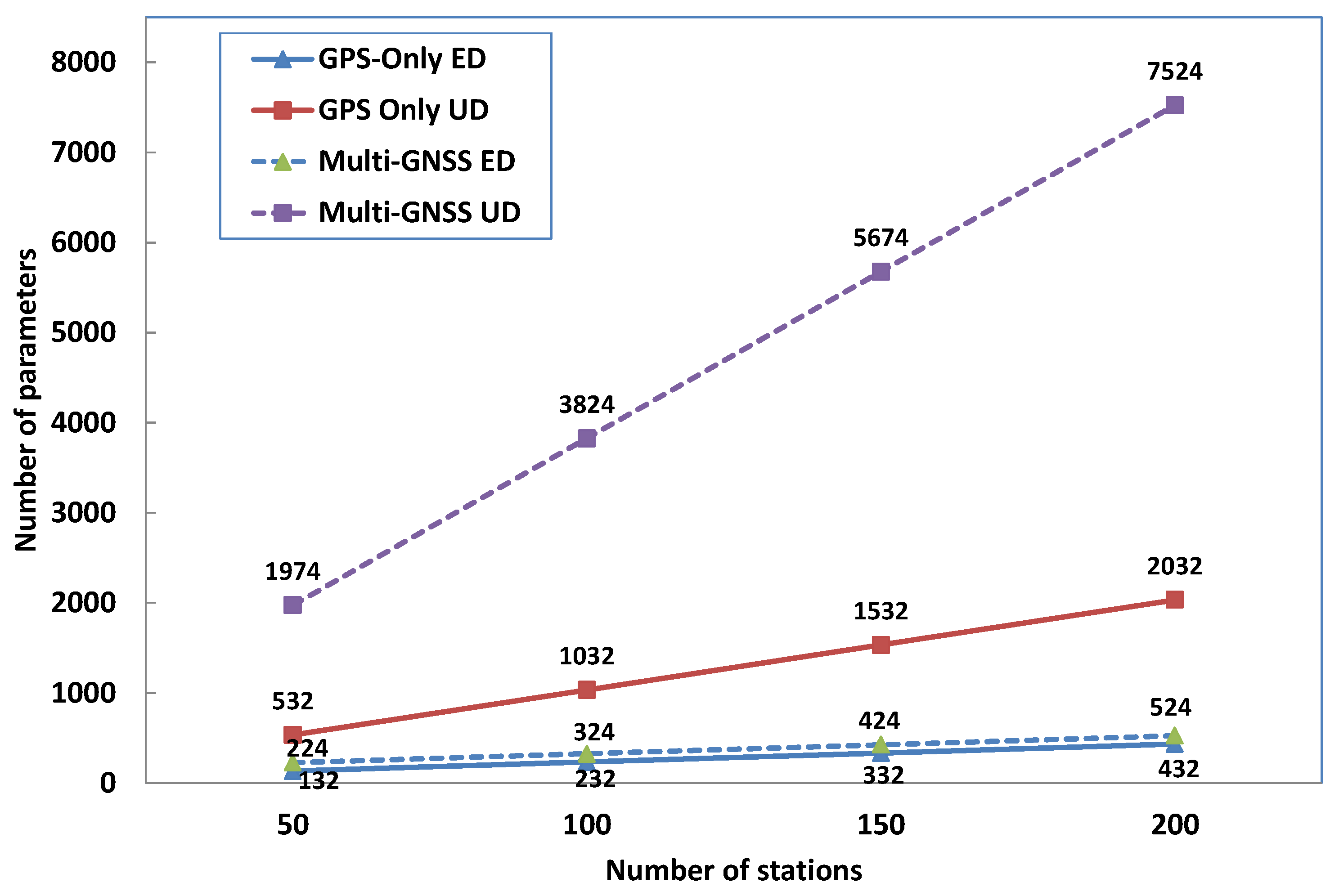
2.4. Parameter Estimation Methodology

In this contribution, we use Square Root Information Filter (SRIF) to estimate real-time clock parameters both in UD and ED models. SRIF is an enhanced Kalman filter, which is suggested in GNSS data processing as it is numerically stable. The core principle of SRIF is to update the filter state using the Householder orthogonal transformation [28]. The a priori information of the state can be expressed as

$${\tilde{\mathrm{z}}}_i={\tilde{\mathrm{R}}}_i{\mathrm{x}}_i+{\tilde{\mathrm{v}}}_i,$$

(10)

where ${[\tilde{\mathrm{R}}}_i{,\tilde{\mathrm{z}}}_i]$ is the a prior square root information array, ${\tilde{\mathrm{v}}}_i$ is the noise of the equation noise, and ${\mathrm{x}}_i$ is the state vector. The measurement update with the new observation ${\mathrm{z}}_i={\mathrm{A}}_i\mathrm{x}+{\mathrm{v}}_i$ at epoch i can be expressed as

$$T\left[\begin{array}{c}{\tilde{\mathrm{R}}}_i\\ {\mathrm{A}}_i\end{array}\right]\mathrm{x}=T\left[\begin{array}{c}{\tilde{\mathrm{z}}}_i\\ {\mathrm{z}}_i\end{array}\right]-T\left[\begin{array}{c}{\tilde{\mathrm{v}}}_i\\ {\mathrm{v}}_i\end{array}\right]\Rightarrow \left[\begin{array}{c}{\hat{\mathrm{R}}}_i\\ 0\end{array}\right]\mathrm{x}=\left[\begin{array}{c}{\hat{\mathrm{z}}}_i\\ {\mathrm{e}}_i\end{array}\right]-\left[\begin{array}{c}{\hat{\mathrm{v}}}_i\\ {\mathrm{v}}_e\end{array}\right],$$

(11)

where ${\mathrm{A}}_i$ is the coefficient matrix, ${\mathrm{z}}_i$ is the observation vector, ${\mathrm{v}}_i$ is the corresponding observation error vector, and ${\mathrm{e}}_i$ is the post-fit residual. By using the Household transformation matrix $T$, the a priori information matrix ${\tilde{\mathrm{R}}}_i$ is updated to ${\hat{\mathrm{R}}}_i$. Then the updated state vector can be expressed as

$${\hat{\mathrm{x}}}_i={\hat{\mathrm{R}}}_i^{-1}{\hat{\mathrm{z}}}_i,$$

(12)

Specific to the application of real-time clock estimation, we express state vector ${\hat{\mathrm{x}}}_i$ as two parts which are the constant parameter vector $\mathrm{p}$ and the dynamic parameter vector $\mathrm{y}$ [29]. Considering the state transition equation, we can get the following state equation of ${\mathrm{p}}_{i+1}$ and ${\mathrm{p}}_i$,

$${\mathrm{R}}_w{\mathrm{p}}_{i+1}={\mathrm{R}}_w{\Phi }_{i+1,i}{\mathrm{p}}_i+{\mathrm{R}}_w\mathrm{w},$$

(13)

where $\mathrm{w}$ is the process noise and ${\mathrm{R}}_w$ is the square root of the covariance of $\mathrm{w}$ that is ${\mathrm{R}}_w^{-1}{\mathrm{R}}_w^{-T}=D\left(w\right)$. Based on the Household transformation and similar to Equation (11), we can express the parameter update of real-time clock estimation as

$$T\left[\begin{array}{ccc}{-\mathrm{R}}_w{\Phi }_{i+1,i}& {\mathrm{R}}_w& 0\\ {\hat{\mathrm{R}}}_{p_i}& 0& {\hat{\mathrm{R}}}_{p_{i}y}\\ 0& 0& {\hat{\mathrm{R}}}_y\end{array}\right]\left[\begin{array}{c}{\mathrm{p}}_i\\ {\mathrm{p}}_{i+1}\\ \mathrm{y}\end{array}\right]=T\left[\begin{array}{c}{\mathrm{R}}_w\mathrm{w}\\ {\hat{\mathrm{z}}}_{p_i}\\ {\hat{\mathrm{z}}}_y\end{array}\right]\Rightarrow \left[\begin{array}{ccc}{\tilde{\mathrm{R}}}_{p_i}& {\tilde{\mathrm{R}}}_{p_i{p}_{i+1}}& 0\\ 0& {\tilde{\mathrm{R}}}_{p_{i+1}}& {\tilde{\mathrm{R}}}_{p_{i+1}y}\\ 0& 0& {\tilde{\mathrm{R}}}_y\end{array}\right]\left[\begin{array}{c}{\mathrm{p}}_i\\ {\mathrm{p}}_{i+1}\\ \mathrm{y}\end{array}\right]=\left[\begin{array}{c}{\tilde{\mathrm{z}}}_w\\ {\tilde{\mathrm{z}}}_{p_i}\\ {\tilde{\mathrm{z}}}_y\end{array}\right]$$

(14)

Then, we can predict the state vector as

$$\left[\begin{array}{cc}{\tilde{\mathrm{R}}}_{p_{i+1}}& {\tilde{\mathrm{R}}}_{p_{i+1}y}\\ 0& {\tilde{\mathrm{R}}}_y\end{array}\right]\left[\begin{array}{c}{\mathrm{p}}_{i+1}\\ \mathrm{y}\end{array}\right]=\left[\begin{array}{c}{\tilde{\mathrm{z}}}_{p_i}\\ {\tilde{\mathrm{z}}}_y\end{array}\right]$$

(15)

Based on Equation (15) and the new observations, the real-time clock parameters are estimated in a recursive way epoch by epoch using SRIF.

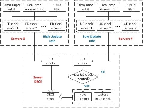
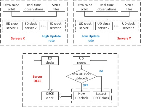
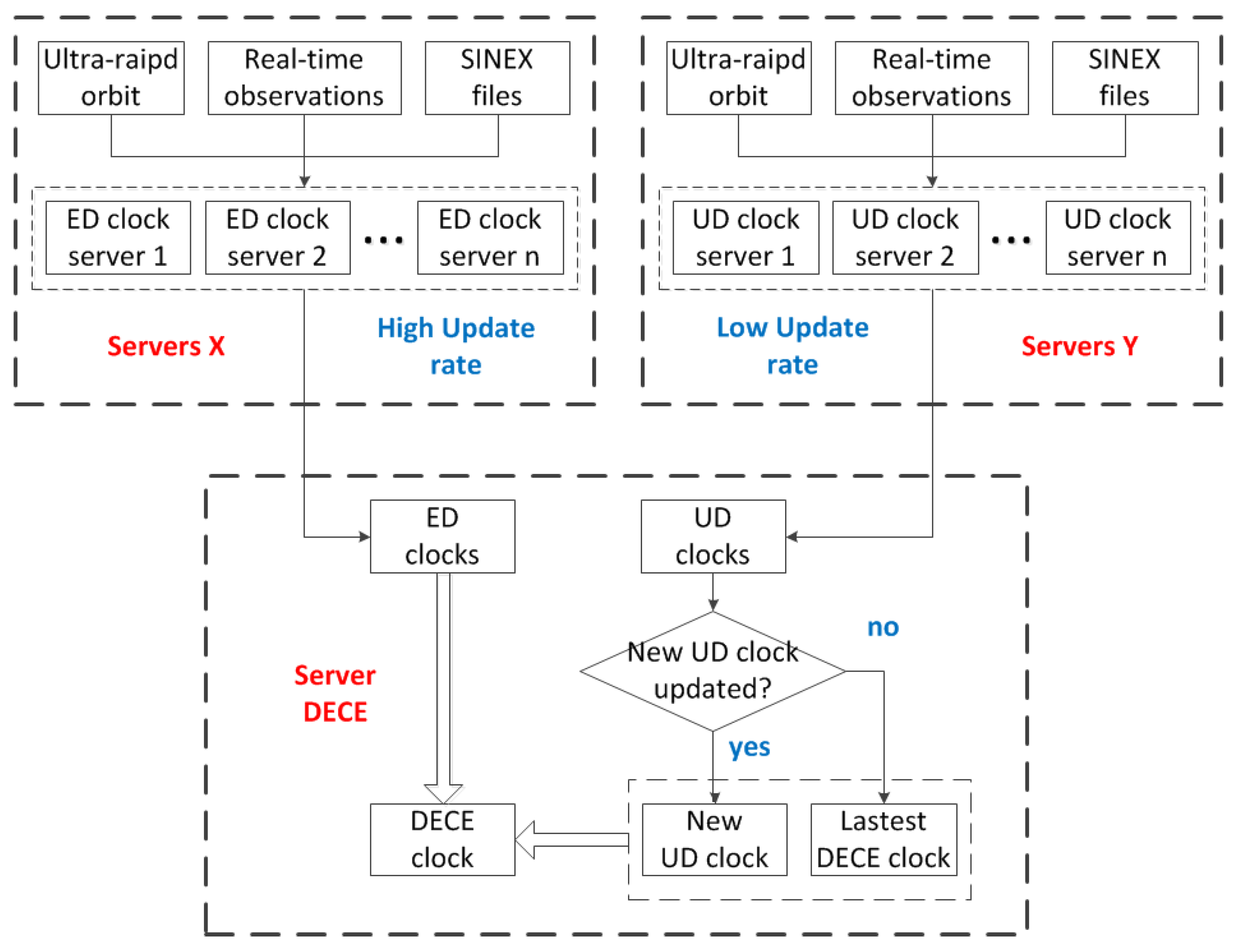
3. Decentralized Clock Estimation (DECE)

Instead of integrating ED and UD and combination processing in a single process in terms of threads, we propose a decentralized clock estimation mode in which UD, ED, and the combination can be run in separated computers with a network connection. Figure 3 shows a flow chart of the simplest DECE configuration with one UD, and one ED and a combination process each running in a server. Ultra-rapid orbit and real-time observations are needed for each server group and we fix site coordinates to Solution INdependent EXchange (SINEX) format solution [30,31]. Both clock products from the ED and UD processes are transferred to the server where the combination is running to generate the final clock products simultaneously according to Equation (9). It should be noted that the orbit switching on each server is synchronous.

One of the advantages of the DECE is that the data exchange among the processes is very small and mainly for transmitting the estimated clocks, and thus can be easily realized through a TCP/UDP port. A much more important advantage is that DECE can significantly improve the robustness of the real-time precise positioning service by running redundant processing processes.

Although only two clock estimation processes are deployed in Figure 3 and used in this study, it can be extended to include more with the same strategy and stations as redundant processing.

Processing processes with different strategies or different station sub-networks can also be involved for using more stations. All the processing processes can be deployed in servers either of a local network or in an offsite network. The combination processes automatically collect the necessary clock estimates according to specified weights to generate a combined product. It is obvious that the robustness of the processing or the availability of the clock products can be dramatically improved by such a distributed system, as the system can always provide high-rate clock product if one of the redundant ED solutions and one of the redundant UD solutions are working well. The crash of the clock combination process is negligible, since it can provide well-qualified combined clocks instantaneously after restarting.

4. Real-Time Experimental Evaluation

In order to validate the DECE strategy, we use the Position and Navigation Data Analyst (PANDA) software package [25,26] as the base, and the real-time estimator is adapted to a distributed environment and a tool for real-time clock combinations developed for the DECE processing. First, we describe the whole data processing of the real-time precise positioning service based on the PANDA software package, and then the network and finally the processing parameters and processing schema used in the validation.

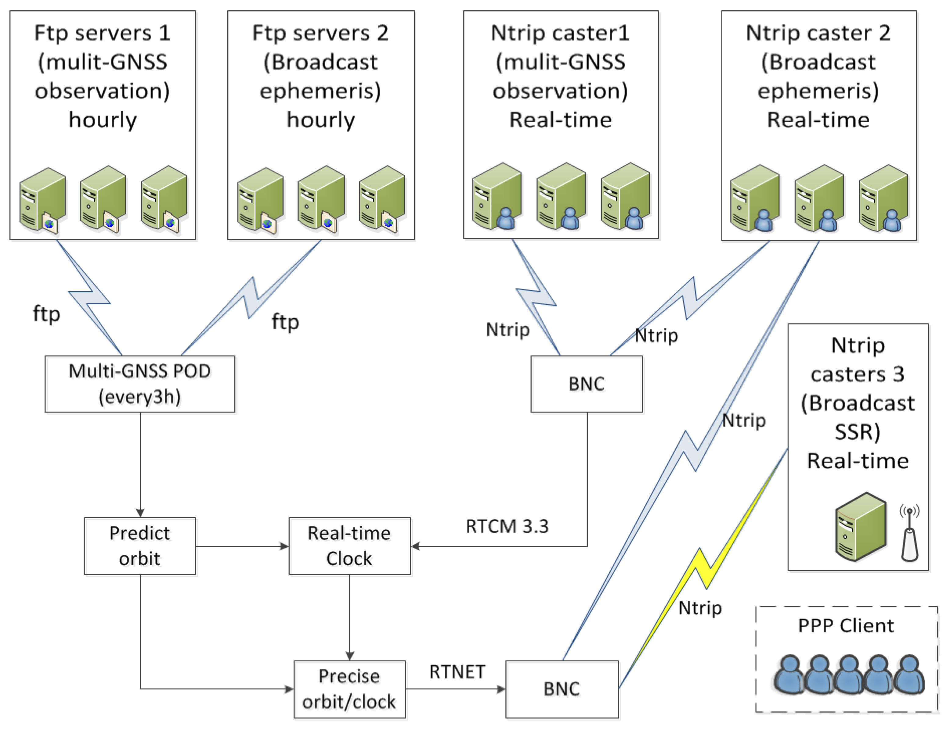
4.1. Data Processing System

In our system, the real-time Precise Orbit Determination (POD) is carried out in batch-processing mode using the observations from MGEX and IGS networks. All parameters in PDO are estimated by least squares adjustment and previous 24-h observations are used to generate the rapid orbit. Then the real-time orbit is predicted based on the rapid orbits in a batch-processing mode by using orbit integrator for at least six hours in a similar way to that of the IGS ultra-rapid data processing. Then the real-time clock estimation processes will do parameter estimation epoch by epoch based on the fixed real-time orbit using the methodology introduced in Section 2.4.

The BKG Ntrip Client (BNC) software (version 2.12) [32] is used to receive real-time observations as well as ephemeris data to feed the filter for clock estimation, and is also used to generate state-space representation corrections from the estimated orbits and clocks. Real-time data are transported using the NTRIP protocol and encoded/decoded following the RTCM 3.3 standard [11]. The structure of all systems is shown in Figure 4.

In order to evaluate the performance of the DECE processing strategy, the “Real-time Clock” function in Figure 4 can be replaced by a single UD processing or by the DECE in Figure 3 to carry out UD processing and DECE processing for comparison.

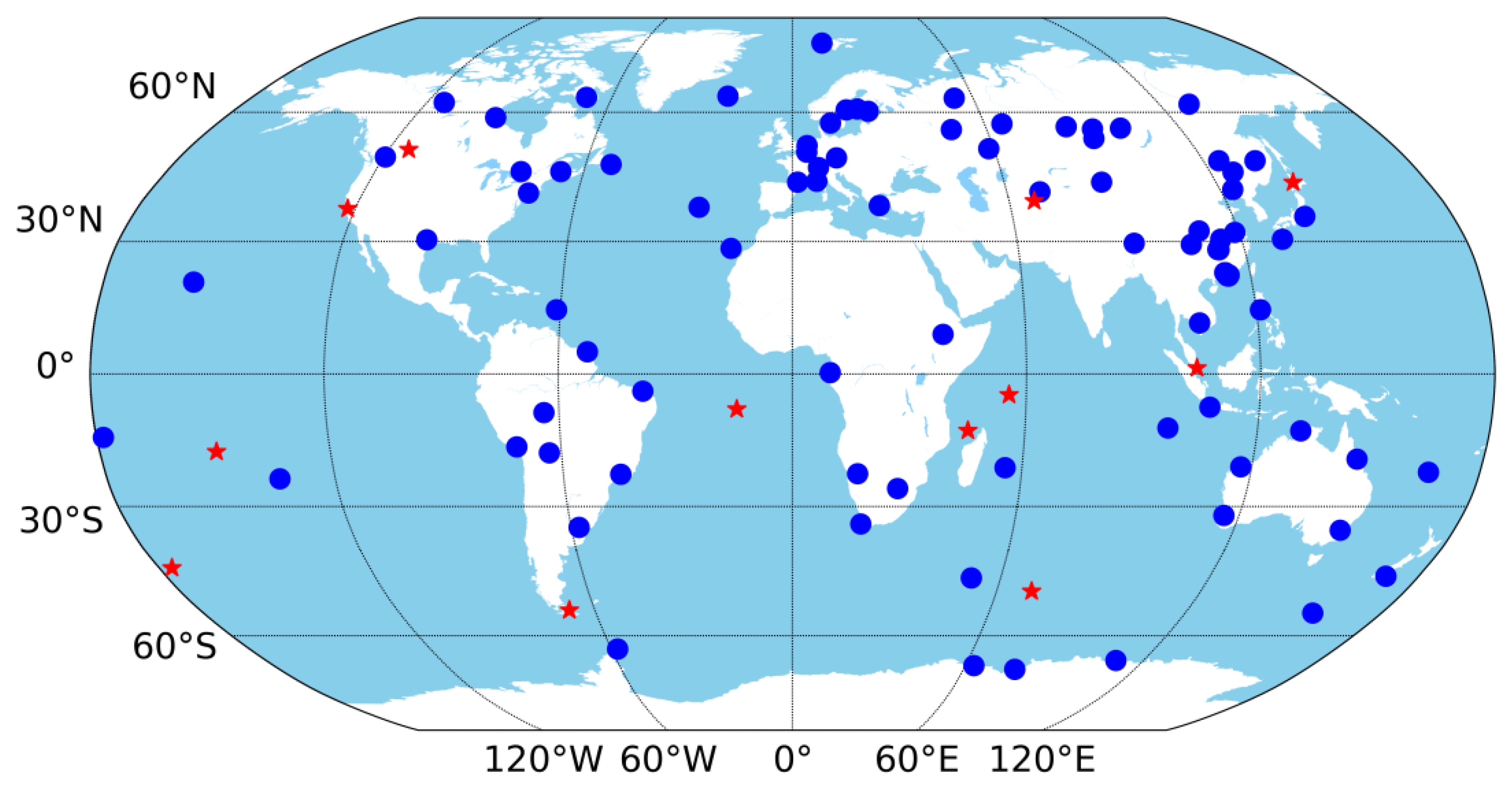
4.2. Data and Network

A network of about 110 global multi-GNSS stations is employed in the experiment. All the 110 stations can track GPS signals, while 105, 65, and 83 stations are with GLONASS, Galileo, and BeiDou tracking capacity, respectively. Most of the real-time observation streams are provided by the International GNSS Service (IGS) and the Multi-GNSS Experiment (MGEX). German Geoscience Research Center (GFZ) and the German Federal Agency for Cartography and Geodesy (BKG) also contributed some multi-GNSS stations. The distribution of the stations is shown in Figure 5. The circle marks are the 110 stations used for clock estimation, while the stars indicate the 12 stations used for real-time PPP test in Section 5.3, which are not included in clock estimation. Because of the network or other reasons, real-time streams are not as stable as the recorded observation files. Normally there are at least 90 stations available for clock estimation.

4.3. Processing Parameters

The data processing parameters are shown in

Table 3. Observation models involved in clock estimation.

Measurement model
Observation	Ionospheric-free combinations of code and phase measurements
Sample rate	Undifferenced (UD) 20s/Epoch-differenced (ED) 5s
Elevation cutoff angle	7°
Weighting	A priori precision of 0.03 cycles and 3.0 m for raw phase and code, respectively, 1 for E > 30 otherwise 2sin(E) [33]
Systematic error
Receiver phase center	igs14.atx(Phase Center Offset (PCO) and Phase Center Variation (PCV) of Galileo and Beidou are corrected as Global Positioning Systems (GPS)
Satellite phase center	igs14.atx(PCO and PCV of Galileo and Beidou are corrected as GPS
Phase wind up	Corrected [34]
Troposphere a priori model	Saastamoinen model for wet and dry hydrostatic delay with Global Mapping Function (GMF) mapping functions without gradient model [35]
Solid Earth tides	IERS Conventions 2010 [36]
Solid Earth pole tides	IERS Conventions 2010
Ocean tides	IERS Conventions 2010
Relativistic effects	IERS Conventions 2010
Stochastic model
Adjustment method	SRIF
Station coordinate	Fixed (from SINEX file or by Position and Navigation Data Analyst (PANDA) GPS-only PPP weekly solutions)
Satellite orbit	Fixed (from predicted orbit)
Receiver clocks	White noise with a unit weight variance of 9000 m
Satellite clocks	White noise with a unit weight variance of 5000 m
Ambiguity	Estimated as constant parameters and re-initialized if a cycle slip, loss of lock and other data disruption occurs/None for ED
Troposphere	Piecewise constant zenith delay for each station every 2 h with a constraint of 2 cm/√h
Inter-System Bias (ISB)	Estimated as constant/None for ED
Inter-Frequency Phase Bias (IFB)	Estimated in the orbit determination and corrected as a constant

and are kept the same for both UD and ED mode if it is not specified. It should be mentioned that there is no official Phase Center Offset (PCO) and Phase Center Variation (PCV) information for Beidou and Galileo satellite and receiver antennas at present, so we use GPS antenna parameters instead.

5. Results

The experimental real-time precise positioning service has been run operationally and we take the orbit and DECE clock products from Day of Year (DOY) 274 to 280, 2018 for the validation. In the experiment, we use a 5-s update rate for ED clock estimator and 20 s for UD clock estimator to generate 5 s final DECE clock products. The CPU we used is Intel(R) Xeon(R) CPU E5-2637 v4 @ 3.50GHz.

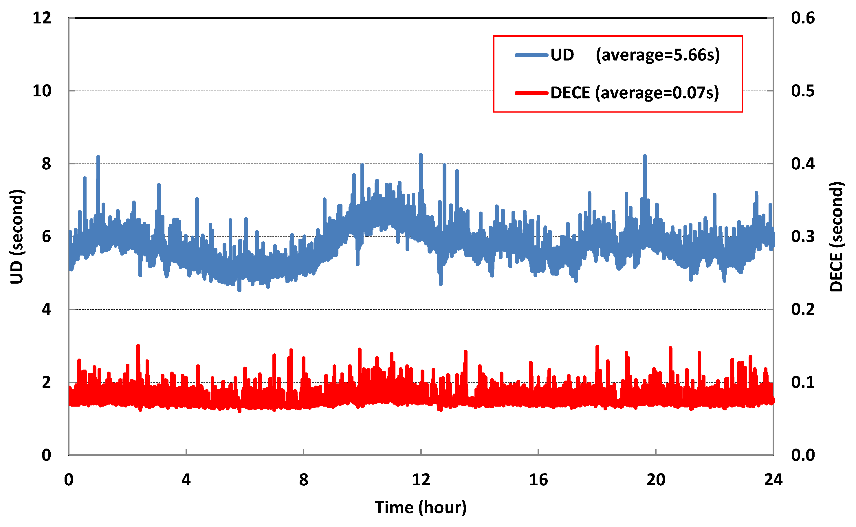
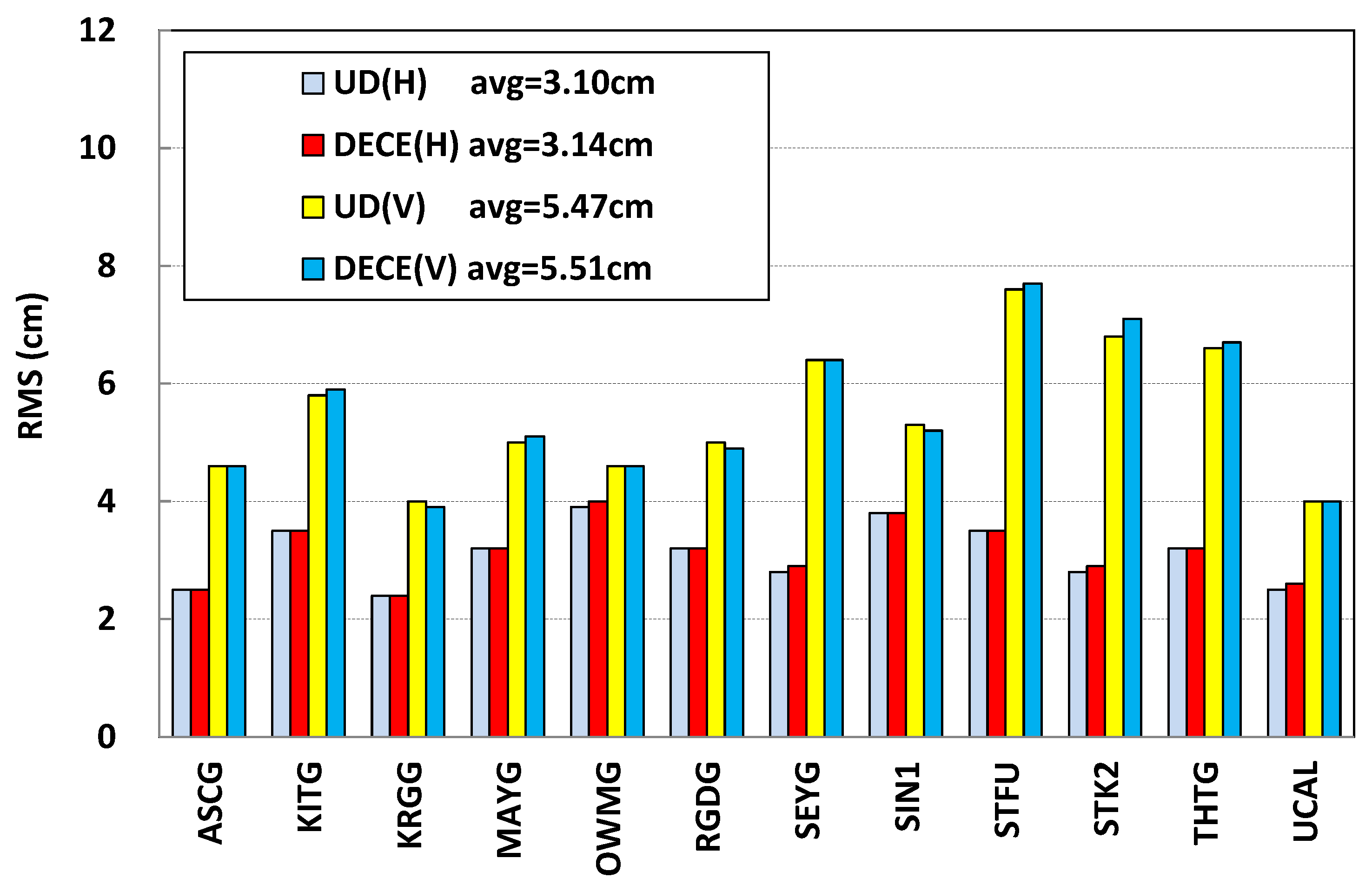
5.1. Decentralized Clock Estimation (DECE) Compared to Undifferenced (UD)

Taking the results of DOY 251 in 2018 as an example, Figure 6 shows the time consumed using UD and DECE at each epoch. The computing time of the DECE is 0.07 s on average, which is much less than that of the UD mode, which is about 5.66 s. It should be noted that it is difficult to update the UD clock within five seconds at each epoch, especially when quality control is involved. What is more, with the completion of Galileo and Beidou in the near future, 124 satellites will be used and the burden of calculation will further increase. On the contrary, the DECE model can solve this computational problem easily.

According to the combination algorithm described by (9), the difference between DECE and UD clocks is mainly caused by the non-synchronization of the clock datum. Taking the results of DOY 251 in 2018 as an example, Figure 7 shows the time series of differences between the DECE and UD products and each subplot shows the differences of all satellites of one system.

From the results, it is obvious that most of the differences between DECE and UD are very subtle, normally smaller than 0.02 nsec (about 6 mm). For multi-GNSS real-time PPP, the influence of such differences can be ignored.

Figure 8 shows the detailed behavior of the difference between the UD and the DECE results, which takes a 5-min time series as an example. Since the interval of UD results is 20 s, which cannot fit with the 5-s DECE clock at each epoch, the linear interpolation has implemented to the UD clock to ensure there is always a corresponding point fit to DECE. In addition, it will not be clear enough if the results of many satellites are plotted together in one figure, so here we plot the single satellite’s series and take G02 and G06 as an example for analysis.

Figure 8 is interesting because there appears to be a periodical slip every 4 epochs (20 s) in the series, but not always obviously. This is probably because normally the DECE process needs to adjust to the UD process as a datum every 4 epochs. According to the combination methodology described in Section 2.3, the difference between DECE and UD clocks present in the series is mainly caused by the non-synchronization of the clock datum. However, more detailed property of these slips still needs further research.

5.2. Decentralized Clock Estimation (DECE) Compared to Post-Processing Products

As for further evaluation of the DECE products, they are also compared with the MGEX final products provided by GFZ (GBM) which is supposed to have the best quality among the existing multi-GNSS products [37]. The clock difference and the Signal-In-Space Ranging Error (SISRE) which is a measure of the joint effect of orbits and clocks will be analyzed below.

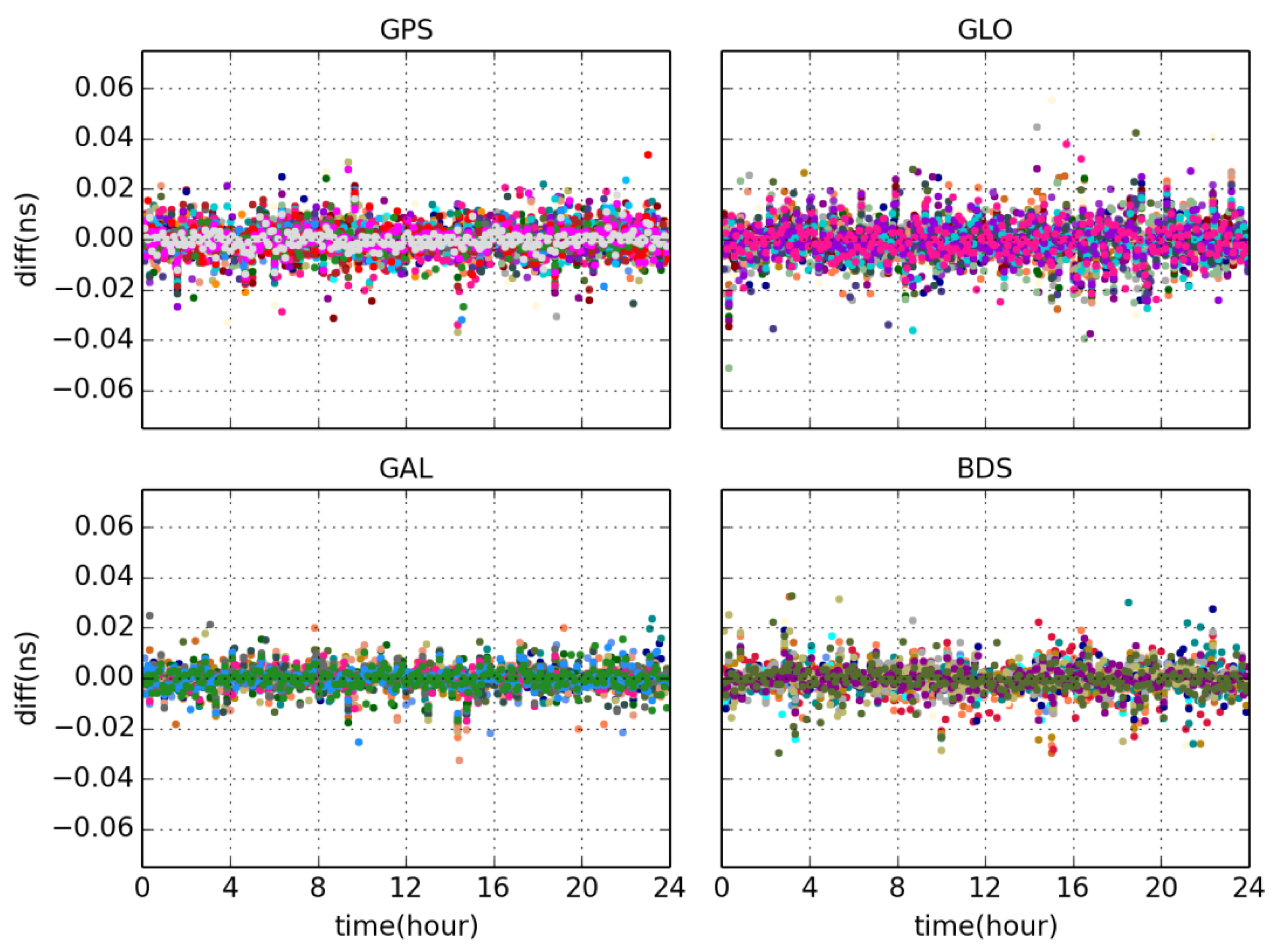
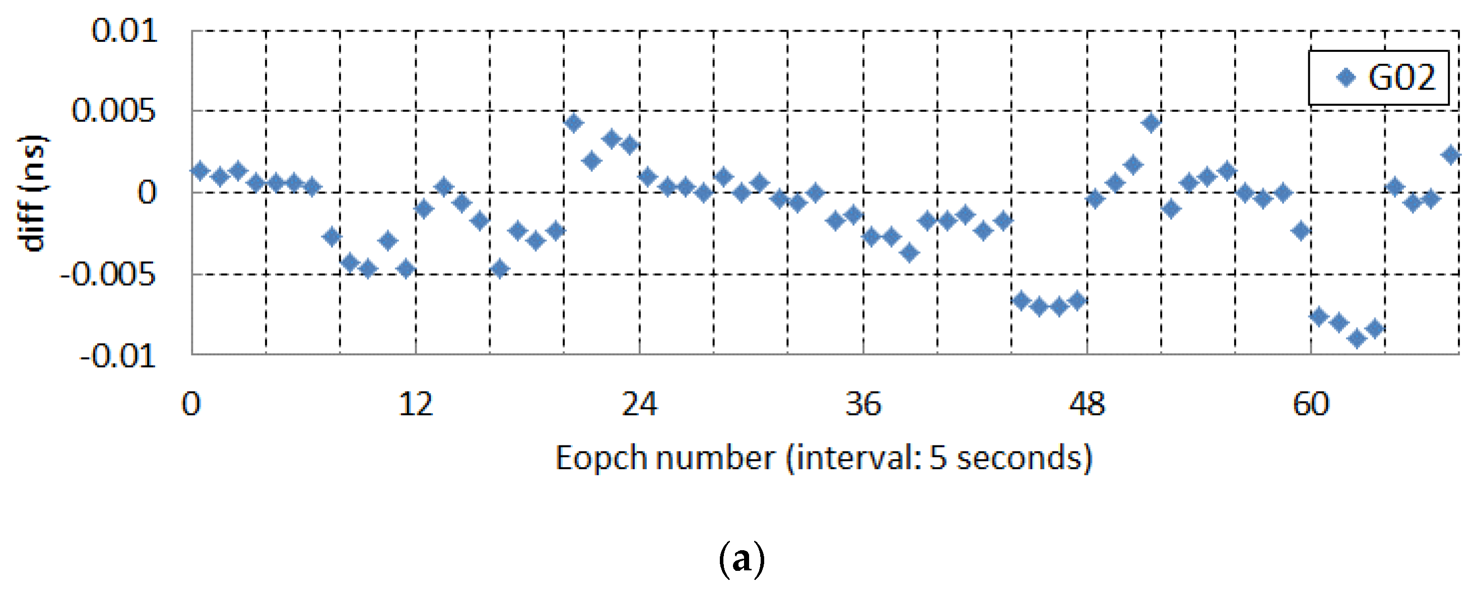
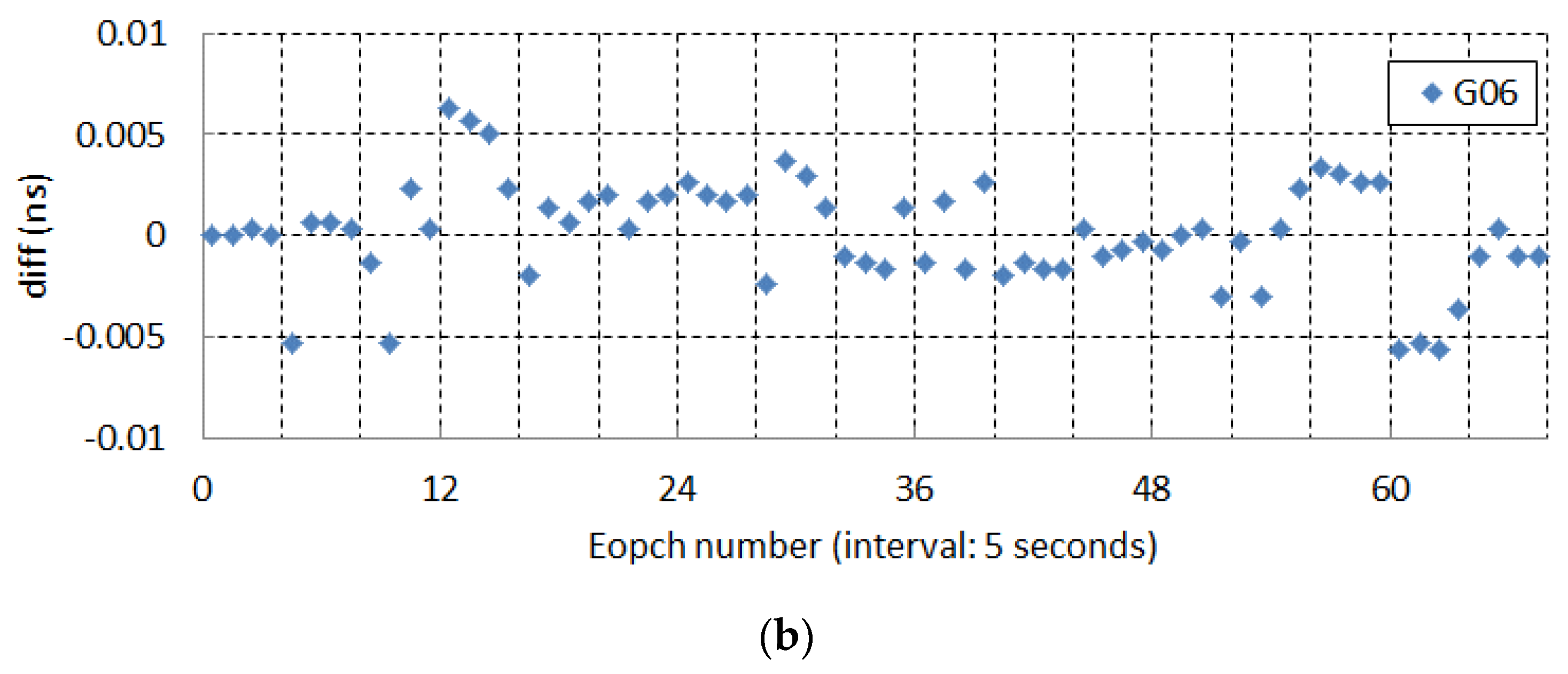
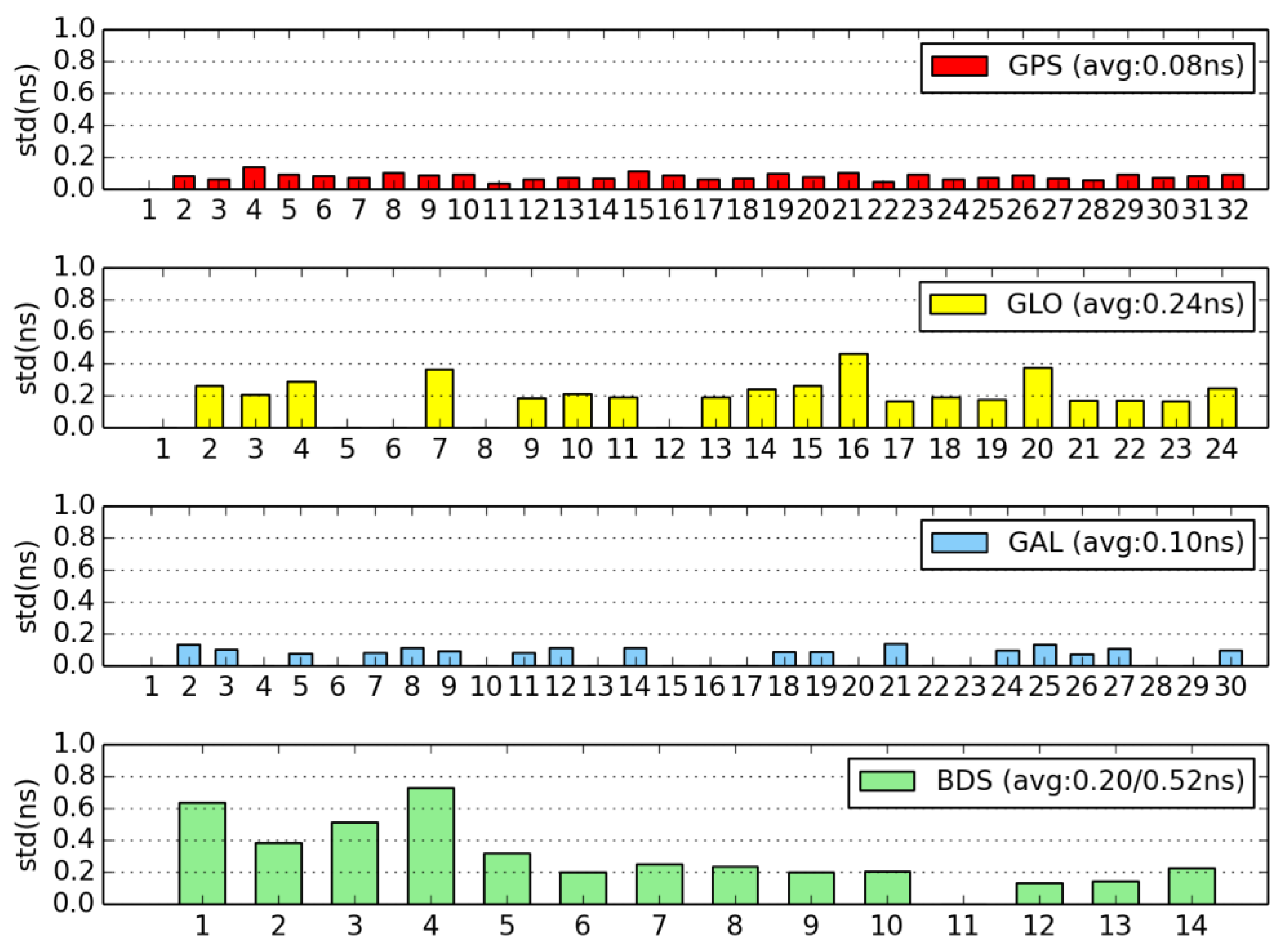
5.2.1. Clock Difference

Since receiver and satellite clocks are estimated epoch-wise as white noise, the clock datum could change from epoch to epoch and the inter-system range bias at receivers could also induce inter-system clock biases. Therefore, in the multi-GNSS clock comparison, a satellite clock from each system is selected as a reference, and single-differenced clocks with respect to the reference satellites are used, in which the datum differences between different products are removed. Here G01, R01, E01, and C11 are selected as the reference satellite for each system, respectively.

As the bias in the time series of the between-satellite clock differences can be absorbed by ambiguities in PPP, the Standard Deviation (STD) of the clock is a significant indicator to reflect the impact of the clock on phase-based positioning. STD values of the differenced clocks are calculated for each satellite and shown in Figure 9. Each subplot in Figure 9 is for a system indicated inside the $i$th system averaged STD value. For BDS to the left and right of the slash means the value for MEO/IGSO and GEO, respectively.

From the statistical results above, it can be seen that the average STD of GPS is 0.08 nsec, while GLONASS, Galileo, BDS MEO/ISO, and BDS GEO are 0.24 nsec, 0.10 nsec, 0.20 nsec, and 0.52 nsec, respectively. The main reason for the larger difference of BDS GEO satellites is due to the insufficient tracking stations and the poor tracking geometry.

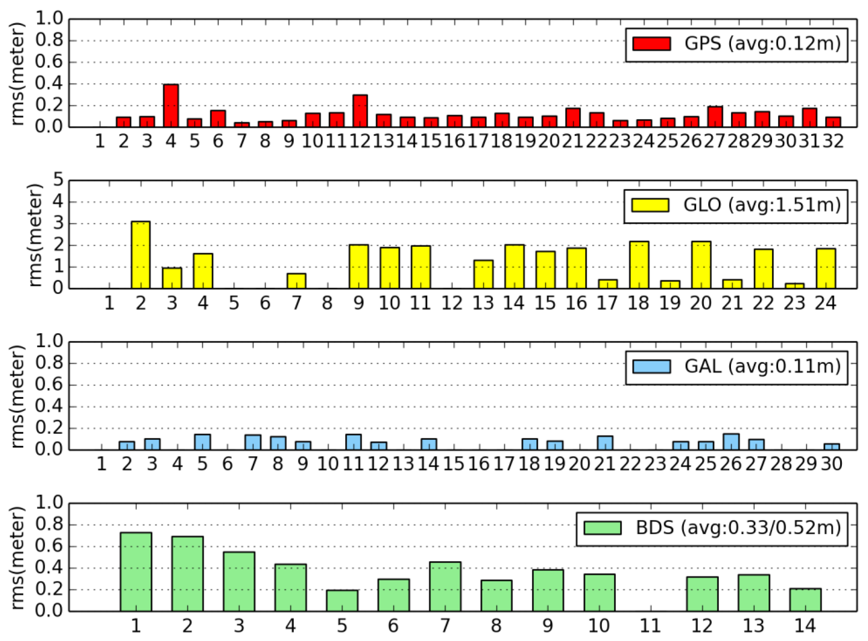
5.2.2. Signal-in-Space Ranging Error (SISRE)

In the clock estimation, most of the orbit biases in the radial direction can be absorbed by clock parameters. This means that satellite clocks are biased by orbit biases in the radial direction and the biases are complementary. The SISRE is a statistical measure for the impact of orbit and clock errors on the modeled pseudorange. The SISRE takes the orbit differences into consideration while comparing clocks of two products by projecting their satellite position difference on the line-of-sight direction from satellite to the user position. It is introduced as a more reliable indicator of the comprehensive influence of orbits and clocks. The formula of SISRE is given by Montenbruck et al. [38] as

$$SISRE=\sqrt{{(a\ast dR-C\ast dt)}_{}^2+b\ast {(dA+dC)}_{}^2},$$

(16)

where $dR$, $dA$, and $dC$ represent the orbit differences in radial direction, along direction, and cross directions, while $dt$ denotes the real-time clock error compared to final products, $C$ is the speed of light in vacuum, $a$ and $b$ represent the SISRE coefficient according to satellite altitude. The coefficients for multi-GNSS SISRE are shown in

Table 4. Coefficient of Signal-in-Space Ranging Error (SISRE).

System	a	b
Global Positioning System (GPS)	0.98	1/41
GLONASS	0.98	1/45
Galileo	0.98	1/61
BeiDou(MEO/IGSO)	0.98	1/54
BeiDou(GEO)	0.99	1/126

[38]. Obviously, we can find that the SISRE is mostly affected by the radial direction orbit difference and clock difference.

The results of SISRE are shown in Figure 10. From the statistical results above, it can be seen that the Root Mean Square (RMS) of SISRE for GPS is 0.12 m, while GLONASS, Galileo, BDS MEO/ISO, and GEO 1.51 m, 0.11 m, 0.33 m, and 0.52 m, respectively. The SISRE of GLONASS is significantly larger than for other systems probably due to frequency division multiple access (FMDA) which needs further research. It should be noted that the SISRE mainly reflects the influence of the products on pseudorange positioning.

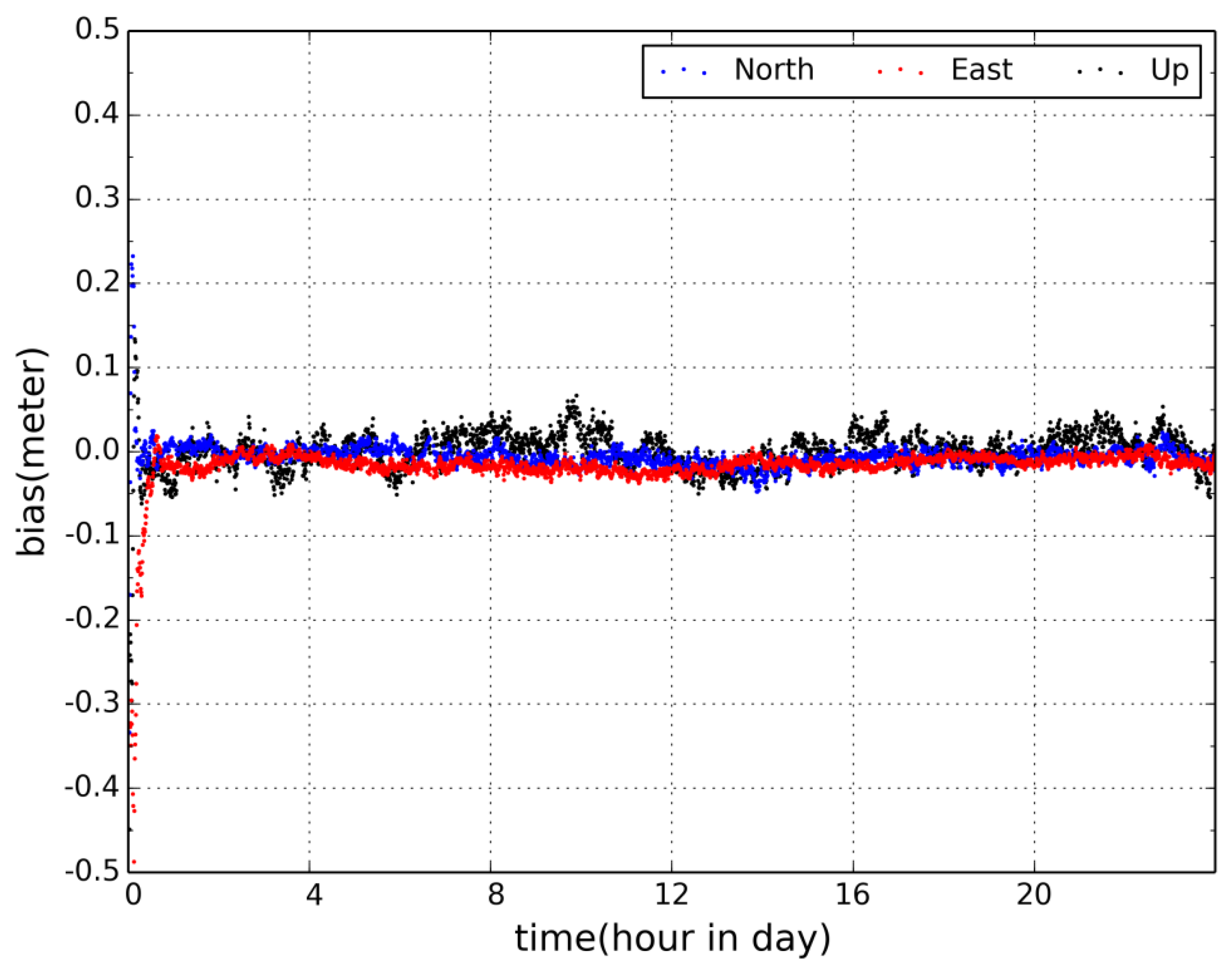
5.3. Precise Point Positioning (PPP) Validation

PPP is a convincing way to directly verify the orbit and clock products together. In the experiment, real-time kinematic PPP is also carried out for 12 global multi-GNSS stations from MGEX using the DECE products and the UD products, respectively. The data processing strategy and parameter model are the same as in Table 3, except that the satellite clock is fixed in PPP and coordinates are estimated in the kinematic mode as white noise. The real-time streams come from mgex.igs-ip.net:2101 and the sample rate is set to five seconds. PPP for all stations is processed using multi-GNSS observations.

Figure 11 illustrates the positioning error of the station ASCG in the north, east, and vertical components. The figure shows that the positioning accuracy of PPP with the DECE clock in a real-time mode is better than 10 cm in the horizontal and 20 cm in the vertical after initialization, which can meet the need most positioning applications. Similar accuracies were obtained for the other stations.

The RMS is an important indicator for evaluating the positioning performance which can be calculated as

$$RMS=\sqrt{\frac{{\displaystyle \sum _{i=1}^n{(X_{ppp}-X_{ref})}^2}}{n}},$$

(17)

where $X_{ppp}$ and $X_{ref}$ represent any of the calculated and reference coordinates and $n$ is the epoch number used for PPP.

In the experiment, the RMS of the position differences using DECE and UD products are shown in Figure 12, in which the legend H and V mean horizontal and vertical direction, respectively. All results are counted after PPP convergence. The statistics show that the average RMS is about 3.10 cm for using UD and 3.14 cm for DECE in horizontal, and 5.47 cm for using UD and 5.51 cm for DECE in vertical. In general, for PPP, centimeter-level positioning results can be achieved using the clock products. Normally the result of UD is a little better than DECE, but there is almost no difference in the accuracy between using DECE and UD products.

6. Discussion

With the great progress of multi-GNSS real-time PPP, the performance of real-time clock products becomes more and more important. Different from post-processing and near-RT modes, the computational efficiency of real-time clock estimation is critical, because the delay or missing of the products will directly affects the positioning accuracy of the PPP client. Moreover, since the recovery of real-time service normally takes a lot of time, especially in case of software crashes, higher requirements for the stability and continuously of real-time products are also necessary. In Section 3, to solve the problems above, we proposed a DECE strategy to improve the computational efficiency and enhance the robustness of the real-time system. First, both low-rate UD and high-rate ED processes are implemented to guarantee the timely update of real-time clock products. From Figure 1 and Figure 7, it is noted that although with the launch of more new satellites and setup of more ground GNSS stations in near future, the processing pressure will still not increase significantly. In addition, when using the DECE strategy, more than one line can be the processed in different processing centers or processing using different strategies (ED/UD). This means the robustness of the processing or the availability of the clock products can be significantly improved by such a distributed system, as the system can always provide high-rate clock products if one of the redundant ED solutions and one of the redundant UD solutions are both working well. As the PPP experimental results show in Section 5.3, centimeter accuracy position can be achieved using the DECE real-time products, which is a great improvement of computational efficiency and robustness. It also improves the experience of real-time positioning users.

7. Conclusions

We proposed the decentralized clock estimation approach to improve the computational efficiency and robustness of the real-time precise positioning service. In the new approach, both the UD and ED modes are implemented but run separately in different computers. The UD mode estimates clock offsets with a lower update rate because a great number of ambiguities parameters are included, while the ED mode determines clock variations with a higher update rate. The products of the two modes are combined to generate the final products. Redundant UD and/or ED processing lines can be scheduled even in offsite computers with an internet connection to improve the robustness of the processing system. More processing lines for different networks can also be included to improve the clock quality.

The new approach is realized for the experimental evaluation based on the PANDA software package for GNSS data processing and BNC software for data communication. The experiment was carried out in real time with about 110 stations for clock estimation and 12 stations for PPP. The clock comparison of the new approach with GFZ MGEX product shows that the STD of GPS is 0.08 nsec, while GLONASS, Galileo, BDS MEO/ISO, and BDS GEO are 0.24 nsec, 0.10 nsec, 0.20 nsec, and 1.52 nsec, respectively. The STD of signal-in-space range error (SISRE) of the clock product of GPS is 0.02 m, while GLONASS, Galileo, BDS MEO/ISO, and BDS GEO are 1.51 m, 0.11 m, 0.33 m, and 0.52 m, respectively. Using the estimated clocks and corresponding orbit products, real-time kinematic multi-GNSS precise point positioning can be realized with an averaged RMS of about 3.14 cm in horizontal and 5.51 cm in vertical.

All these results confirm that the decentralized clock estimation can provide comparable clock products as the most used undifferenced method but with a much higher computational efficiency and robustness. It is a suitable approach for multi-GNSS real-time clock estimation with the increasing number of satellites and stations and signals of different frequency bands.

References

1. Malys, S.; Jensen, P.A. Geodetic point positioning with GPS carrier beat phase data from the CASA UNO experiment. Geophys. Res. Lett. 1990, 17, 651–654. [Google Scholar] [CrossRef]
2. Zumberge, J.F.; Heflin, M.B.; Jefferson, D.C.; Watkins, M.M.; Webb, F.H. Precise point positioning for the efficient and robust analysis of GPS data from large networks. J. Geophys. Res. 1997, 102, 5005–5017. [Google Scholar] [CrossRef] [Green Version]
3. Bisnath, S.; Gao, Y. Current state of precise point positioning and future prospects and limitations. In Observing our Changing Earth. International Association of Geodesy Symposia; Sideris, M.G., Ed.; Springer: Berlin/Heidelberg, Germany, 2009; Volume 133. [Google Scholar] [CrossRef]
4. Geng, J.; Shi, C.; Ge, M.; Dodson, A.; Lou, Y.; Zhao, Q.; Liu, J. Improving the estimation of fractional-cycle biases for ambiguity resolution in precise point positioning. J. Geodesy 2012, 86, 578–589. [Google Scholar] [CrossRef]
5. Ge, M.; Gendt, G.; Rothacher, M.; Shi, C.; Liu, J. Resolution of GPS carrier-phase ambiguities in precise point positioning (PPP) with daily observations. J. Geodesy 2008, 82, 389–399. [Google Scholar] [CrossRef]
6. Li, X.; Ge, M.; Dai, X.; Ren, X.; Fritsche, M.; Wickert, J.; Schuh, H. Accuracy and reliability of multi-GNSS real-time precise positioning: GPS, GLONASS, BeiDou, and Galileo. J. Geodesy 2015, 89, 607–635. [Google Scholar] [CrossRef]
7. Lou, Y.; Zheng, F.; Gu, S.; Wang, C.; Guo, H.; Feng, Y. Multi-GNSS precise point positioning with raw single-frequency and dual-frequency measurement models. GPS Solut. 2016, 20, 849–862. [Google Scholar] [CrossRef]
8. Liu, Y.; Lou, Y.; Ye, S.; Zhang, R.; Song, W.; Zhang, X.; Li, Q. Assessment of PPP integer ambiguity resolution using GPS, GLONASS and BeiDou (IGSO, MEO) constellations. GPS Solut. 2017, 21, 1647–1659. [Google Scholar] [CrossRef]
9. Li, X.; Ge, M.; Dousa, J.; Wickert, J. Real-time precise point positioning regional augmentation for large GPS reference networks. GPS Solut. 2014, 18, 61–71. [Google Scholar] [CrossRef]
10. Liu, T.; Yuan, Y.; Zhang, B.; Wang, N.; Tan, B.; Chen, Y. Multi-GNSS precise point positioning (MGPPP) using raw observations. J. Geodesy 2017, 91, 253–268. [Google Scholar] [CrossRef]
11. RTCM. Radio Technical Commission for Maritime Services (RTCM) Standard 10403.3, Differential GNSS (Global Navigation Satellite Systems) Services; Radio Technical Commission for Maritime Services: Arlington, VA, USA, 2016. [Google Scholar]
12. Kouba, J.; Héroux, P. Precise point positioning using IGS orbit and clock products. GPS Solut. 2001, 5, 12–18. [Google Scholar] [CrossRef]
13. Griffiths, J.; Ray, J. On the precision and accuracy of IGS orbits. J. Geodesy 2009, 83, 277–278. [Google Scholar] [CrossRef]
14. Shi, C.; Guo, S.; Gu, S.; Yang, X.; Gong, X.; Deng, Z.; Ge, M.; Schuh, H. Multi-GNSS satellite clock estimation constrained with oscillator noise model in the existence of data discontinuity. J. Geodesy 2019, 93, 515–528. [Google Scholar] [CrossRef]
15. Bock, H.; Dach, R.; Jäggi, A.; Beutler, G. High-rate GPS clock corrections from CODE: Support of 1 Hz applications. J. Geodesy 2009, 83, 1083–1094. [Google Scholar] [CrossRef]
16. Zhang, X.; Li, X.; Guo, F. Satellite clock estimation at 1 Hz for realtime kinematic PPP applications. GPS Solut. 2011, 15, 315–324. [Google Scholar] [CrossRef]
17. Ge, M.; Chen, J.; Douša, J.; Gendt, G.; Wickert, J. A computationally efficient approach for estimating high-rate satellite clock corrections in realtime. GPS Solut. 2012, 16, 9–17. [Google Scholar] [CrossRef]
18. Chen, L.; Zhao, Q.; Hu, Z.; Jiang, X.; Geng, C.; Ge, M.; Shi, C. GNSS global real-time augmentation positioning: Real-time precise satellite clock estimation, prototype system construction and performance analysis. Adv. Space Res. 2017, 61, 367–384. [Google Scholar] [CrossRef]
19. Chen, L.; Song, W.; Yi, W.; Shi, C.; Lou, Y.; Guo, H. Research on a method of real-time combination of precise GPS clock corrections. GPS Solut. 2017, 21, 187–195. [Google Scholar] [CrossRef]
20. Zhang, W.; Lou, Y.; Gu, S.; Shi, C.; Haase, J.S.; Liu, J. Joint estimation of GPS/BDS real-time clocks and initial results. GPS Solut. 2016, 20, 665–676. [Google Scholar] [CrossRef]
21. Gong, X.; Gu, S.; Lou, Y.; Zheng, F.; Ge, M.; Liu, J. An efficient solution of real-time data processing for multi-GNSS network. J. Geodesy 2017, 92, 797–809. [Google Scholar] [CrossRef]
22. Laurichesse, D.; Mercier, F.; Berthias, J.P. Real time GPS constellation and clocks estimation using zero-difference integer ambiguity fixing. In Proceedings of the ION ITM 2009, Anaheim, CA, USA, 26–28 January 2009. [Google Scholar]
23. Laurichesse, D.; Cerri, L.; Berthias, J.P.; Mercier, F. Real time precise GPS constellation and clocks estimation by means of a Kalman filter. In Proceedings of the ION GNSS 2013, Nashville, TN, USA, 16–20 September 2013. [Google Scholar]
24. Mervart, L.; Weber, G. Real-time combination of GNSS orbit and clock correction streams using a Kalman Filter approach. In Proceedings of the ION GNSS 2011, Portland, OR, USA, 20–23 September 2013. [Google Scholar]
25. Liu, J.; Ge, M. PANDA Software and its preliminary result of positioning and orbit determination. Wuhan Univ. J. Nat. Sci. 2003, 8, 603–609. [Google Scholar]
26. Shi, C.; Zhao, Q.; Geng, J.; Lou, Y.; Ge, M.; Liu, J. Recent development of PANDA software in GNSS data processing. In Proceedings of the SPIE Volume 7285, Wuhan, China, 8–30 December 2008. [Google Scholar]
27. Dach, R.; Schaer, S.; Hugentobler, U. Combined multi-system GNSS analysis for time and frequency transfer. In Proceedings of the 20th European Frequency and Time Forum EFTF06, Braunschweig, Germany, 2006. [Google Scholar]
28. Bierman, G.J. The treatment of bias in the square-root information filter/smoother. J. Optim. Theory Appl. 1975, 16, 165–178. [Google Scholar] [CrossRef]
29. Dai, X.; Lou, Y.; Dai, Z.; Qing, Y.; Li, M.; Shi, C. Real-time precise orbit determination for BDS satellites using the square root information filter. GPS Solut. 2019, 23, 45. [Google Scholar] [CrossRef]
30. Ray, J.; Dong, D.; Altamimi, Z. IGS reference frames: Status and future improvements. GPS Solut. 2004, 5, 251–266. [Google Scholar] [CrossRef]
31. Rebischung, P.; Altamimi, Z.; Ray, J.; Garayt, B. The IGS contribution to ITRF2014. J. Geodesy 2016, 90, 611–630. [Google Scholar] [CrossRef]
32. Stürze, A.; Mervart, L.; Weber, G.; Rülke, A.; Wiesensarter, E.; Neumaier, P. The new version 2.12 of BKG Ntrip Client (BNC). Geophys. Res. Abstr. 2016, 18, 12012. [Google Scholar]
33. Gendt, G.; Dick, G.; Reigber, C.H.; Tomassini, M.; Liu, Y.; Ramatschi, M. Demonstration of NRT GPS water vapor monitoring for numerical weather prediction in Germany. J. Meteorol. Soc. Jpn. 2003, 82, 360–370. [Google Scholar]
34. Wu, J.; Wu, S.; Hajj, G.; Bertiger, W.; Lichten, S. Effects of antenna orientation on GPS carrier phase. Manuscr. Geodesy 1993, 18, 91–98. [Google Scholar]
35. Boehm, J.; Niell, A.; Tregoning, P.; Schuh, H. Global mapping function (GMF): A new empirical mapping function based on numerical weather model data. Geophys. Res. Lett. 2006, 33, L07304. [Google Scholar] [CrossRef]
36. Petit, G.; Luzum, B. IERS Conventions 2010; Iers Technical Note 36; Verlag des Bundesamts für Kartographie und Geodäsie: Frankfurt am Main, Germany, 2010; Volume 36, pp. 1–95. [Google Scholar]
37. Deng, Z.; Fritsche, M.; Uhlemann, M.; Wickert, J.; Schuh, H. Reprocessing of GFZ Multi-GNSS Product GBM. In Proceedings of the IGS Workshop, Sydney, Australia, 8–12 February 2016; Available online: http://acc.igs.org/workshop2016/presentations/Plenary_01_06.pdf (accessed on 20 February 2016).
38. Montenbruck, O.; Steigenberger, P.; Hauschild, A. Broadcast versus precise ephemerides: A multi-GNSS perspective. GPS Solut. 2015, 19, 321–333. [Google Scholar] [CrossRef]
Figure 1. Relationship between the number of stations and number of parameters for the solutions using epoch-differenced (ED) or undifferenced (UD) model and for global positioning systems (GPS) or multi-GNSS (global navigation satellite systems).
Remotesensing 11 02595 g001
Figure 2. Undifferenced (UD) and epoch-differenced (ED) processing schema.
Remotesensing 11 02595 g002
Figure 3. Flow chart of the decentralized clock estimation (DECE) with the basic configuration, i.e., one undifferenced (UD), one epoch-differenced (ED), and one combination process, each running in a server.
Remotesensing 11 02595 g003
Figure 4. Flow chart of the real-time precise positioning service system based on the Position and Navigation Data Analyst (PANDA) software package.
Remotesensing 11 02595 g004
Figure 5. Distribution of stations for the Multi-GNSS (global navigation satellite systems) real-time clock estimation marked by cycles and that for precise point positioning (PPP) test by pentagrams.
Remotesensing 11 02595 g005
Figure 6. Computational time at each epoch using undifferenced (UD) and decentralized clock estimation (DECE) modes for Day of Year (DOY) 251, 2018.
Remotesensing 11 02595 g006
Figure 7. Differences between decentralized clock estimation (DECE) clock and undifferenced (UD) clock on DOY 251, 2018.
Remotesensing 11 02595 g007
Figure 8. (a) Detailed differences between decentralized clock estimation (DECE) and undifferenced (UD) clock (G02). (b) Detailed differences between DECE and UD clock (G06).
Remotesensing 11 02595 g008aRemotesensing 11 02595 g008b
Figure 9. STD of clock difference.
Remotesensing 11 02595 g009
Figure 10. Signal-in-space ranging error (SISRE) of decentralized clock estimation (DECE) real-time clock.
Remotesensing 11 02595 g010
Figure 11. Result of real-time precise point positioning (PPP) using decentralized clock estimation (DECE) clock (ASCG).
Remotesensing 11 02595 g011
Figure 12. RMS of real-time precise point positioning (PPP) position differenced with respect to their ground truth using decentralized clock estimation (DECE) and undifferenced (UD) products.
Remotesensing 11 02595 g012