Semi-Coupled Convolutional Sparse Learning for Image Super-Resolution

Abstract

In the convolutional sparse coding-based image super-resolution problem, the coefficients of low- and high-resolution images in the same position are assumed to be equivalent, which enforces an identical structure of low- and high-resolution images. However, in fact the structure of high-resolution images is much more complicated than that of low-resolution images. In order to reduce the coupling between low- and high-resolution representations, a semi-coupled convolutional sparse learning method (SCCSL) is proposed for image super-resolution. The proposed method uses nonlinear convolution operations as the mapping function between low- and high-resolution features, and conventional linear mapping can be seen as a special case of the proposed method. Secondly, the neighborhoods within the filter size are used to calculate the current pixel, improving the flexibility of our proposed model. In addition, the filter size is adjustable. In order to illustrate the effectiveness of SCCSL method, we compare it with four state-of-the-art methods of 15 commonly used images. Experimental results show that this work provides a more flexible and efficient approach for image super-resolution problem.

1. Introduction

Conventional sparse coding [1,2,3] (SC) formulates a signal by a linear combination of a few atoms in a redundant dictionary. When processing the high-dimensional image signals, SC-based models often divide the entire image into local patches and handle them separately since computing on the entire image requires huge computing resources [4,5]. Although the block-wise SC scheme is efficient, it is also true that block-wise operation has limited ability of extracting the global features and thus weakens the continuity of edges and contours, sometimes even blocking artifacts. Under this circumstance, the convolutional sparse coding (CSC) [6,7], also known as deconvolutional networks, is put forward to enhance the description of the global features. In contrast to the conventional SC, the CSC model can decompose an image into a group of convolutions of 2D filters and corresponding feature maps as shown in Figure 1. These 2D filters form a dictionary of CSC, and the feature maps which can be seen as sparse coefficients reflect the activation positions of the filters. In order to extract structural features of the image, the feature maps are constrained by sparse priors. Empirical studies show that CSC can better preserve the global structures of images due to the convolutional operation and it has been widely used in computer vision [8,9,10,11].

Image super-resolution (SR) [12,13,14,15,16,17,18] is an active topic in image processing, which is a typical application of the conventional SC-based models. The task of image super-resolution is to learn the nonlinear mapping between low-resolution (LR) and high-resolution (HR) images for reconstructing the input LR image into a HR image, so that the visual effect will be as good as possible. In training phase, the low-/high-resolution (LR/HR) image pairs are used to learn two coupled dictionaries [19,20] by assuming the coefficients of LR and HR patches are identical. In the testing phase, we first calculate the coefficients of the LR patches with the LR dictionary, then multiply the HR dictionary by the calculated coefficients to the HR patches. On the other hand, CSC can also be applied to the image SR problem [21,22]. It is not difficult to find a correspondence between SC- and CSC-based methods. By assuming the LR and HR feature maps are identical, two coupled filter groups can be learned. Following the pipeline of SC-based methods, the HR image can be synthesized by summing up the convolutions of the HR filters and the feature maps.

Even though SC and CSC achieve great successes in cross-modality synthesis problems [13,22], they both face an intractable problem that their models are enforced to learn identical structures between LR and HR images under the coefficient equivalence assumption, but in fact the structures of HR images are much more complex than that of LR images. The strong coupling limits their synthesis performances. An effective way to weaken the coupling between HR and LR dictionaries is building a transform function between them. Wang et al. [23] used a matrix to map the LR coefficient vector to the HR space in the conventional SC-based model. Similarly, for CSC-based model, Gu et al. [22] constructed a mapping function that trains the function to map LR features to HR space. The above two mapping functions can both be interpreted as linear transformation which has been proven to be limited to the approximation of complex functions.

In this paper, we present a semi-coupled convolutional sparse learning (SCCSL) based SR method which uses convolutions as mapping functions to promote the flexibility of the transformation between LR and HR coefficients. The proposed method has three advantages over the linear transformation-based methods. First, convolution is a non-linear operation that is more suitable than a linear function to describe the complex relationship between LR and HR coefficients. Second, when projecting the LR feature maps to HR space, the proposed method uses neighborhoods within the filter size to calculate the current pixel, which enhances the flexibility of the model. Third, the filter size is adjustable. In the limited case where the filter size is 1 × 1, the proposed model degenerates into the linear model. That means that the linear model is a special case in the proposed semi-coupling model. Like other CSC methods [24,25,26], the proposed method is solved in alternating direction method of multipliers (ADMM) [27,28] framework, and the variables are transformed into Fourier domain in which the final results can be calculated by solving a linear system.

The remainder of the paper is organized as follows: In Section 2, we briefly review the principle, current situation of CSC, and its application in image SR. Section 3 details the proposed SCCSL method and the algorithm for reducing the coupling between low- and high-resolution representations. Experiments and discussion are presented in Section 4. Finally, the conclusion is discussed in Section 6.

2. Convolutional Sparse Coding

SC [1,2,3] aims at seeking a concise and efficient way of representing signals. The basic idea is that a signal can be represented by the linear combination of very few atoms in a redundant dictionary under the sparse assumption. Specifically, consider a redundant dictionary D, SC encodes a signal x by Dα, where α is the sparse coefficient vector. The sparse representation framework has been widely used in computer vision tasks, such as color image restoration [29], robust face recognition [30,31], object detection [32,33], image segmentation [34,35], and image classification [36,37], and has achieved state-of-the-art results. Specifically, supervised dictionary learning has a good application in image classification [38], image super-resolution [39], and audio signal recognition [40], and supervised deep dictionary learning has been successfully used in classification [41] and image quality assessment [42]. However, most of the SC-based methods divide the whole image into small patches and deal with them separately for simplification and efficiency [43], which leads to the absence of continuous structures.

In order to overcome the above drawback of SC, Zeiler et al. [6] proposed a convolutional sparse coding framework to sparsely describe the entire image, as well as preserve the global structures. As shown in Figure 1, CSC framework approximates an image by the summation of convolutions of filters and their feature maps. Let $X\in {ℝ}^{M\times N}$ be an input image an ${\left\{D_k\right\}}_{1\le k\le K}$ be a group of filters with size $s\times s$, thus the encoding formulation of the CSC can be expressed as follows:

$$\underset{{\left\{Z_k\right\}}_{1\le k\le K}}{min}\parallel X-{\displaystyle \sum }_{k=1}^K{D}_k\otimes Z_k{\parallel }_F^2+\lambda {\displaystyle \sum }_{k=1}^K\parallel Z_k{\parallel }_1$$

(1)

where ${\left\{Z_k\right\}}_{1\le k\le K}$ is the feature map of ${\left\{D_k\right\}}_{1\le k\le K}$ and $\lambda$ is a penalty factor. The first term ensures the data fidelity, and the second term uses ${\ell }_1$ norm to sparsely activate the feature maps, in which ${\ell }_1$ norm is the absolute value of the elements and ${\ell }_2$ norm is used as a standard quantity for measuring a vector difference. $\otimes$ is the convolution operation. Unlike the conventional SC model whose dictionary is used to represent the local patches, the CSC model uses the filters as a dictionary which has the ability of representing the global features by convolution operations [44]. In addition, the sparse constraints on the feature maps make the corresponding filters have meaningful structures. It should be noted that CSC is totally different from the extremely popular convolutional neural networks (CNN) [45,46,47,48], although both are related to convolution. As described in Equation (1), the convolutions of CSC are implemented on the filters and the feature maps, the filters can be seen as a dictionary and the feature maps are the codings of the image. Distinctively, the filters act directly on the input image to obtain the feature maps in CNN. In other words, CSC aims at image reconstruction [49,50], while CNN focuses on feature extraction [51].

It is easy to extend the CSC model to the image SR problem. Similar to the SC-based methods, the LR-HR image pairs are required to train LR and HR filters. Suppose that we have a group of LR-HR image pairs ${\left\{\left(X_i,Y_i\right)\right\}}_{1\le i\le S}$ for training, by enforcing that the LR and HR feature maps are identical, we have the following formulation:

$$\begin{array}{cc}\hfill \underset{\begin{array}{c}{\left\{D_k^L\right\}}_{1\le k\le K}\\ {\left\{D_k^H\right\}}_{1\le k\le K}\end{array}}{min}& {\displaystyle {\displaystyle \sum }_{i=1}^S}\parallel X_i-{\displaystyle {\displaystyle \sum }_{k=1}^K}{D}_k^L\otimes Z_k^i{\parallel }_F^2\hfill \\ \hfill +& {\displaystyle {\displaystyle \sum }_{i=1}^S}\parallel Y_i-{\displaystyle {\displaystyle \sum }_{k=1}^K}{D}_k^H\otimes Z_k^i{\parallel }_F^2\hfill \\ \hfill +& \lambda {\displaystyle {\displaystyle \sum }_{i=1}^S}{\displaystyle {\displaystyle \sum }_{k=1}^K}\parallel Z_k^i{\parallel }_1\hfill \\ \hfill s.t. \forall 1\le k\le K& \parallel D_k^L{\parallel }_F^2\le {ϵ}_L, \parallel D_k^H{\parallel }_F^2\le {ϵ}_H\hfill \end{array}$$

(2)

where $D_k^L$ and $D_k^H$ are the LR and HR filters respectively, $Z_k^i$ is the $k$-th feature map of the $i$-th image, ${ϵ}_L$ and ${ϵ}_H$ are two constants which are used to restrain the energy of the filters. Note that each LR image is scaled to the size of the corresponding HR image by bilinear interpolation. Since the LR and HR filters use the same feature maps, their learning structures are highly correlated, limiting the diversity of HR reconstruction. Gu et al. [22] introduced a linear mapping function of LR and HR feature maps to reduce their coupling. In their model, the LR filters and the LR feature maps are learned from the LR training images as follows:

$$\begin{array}{cc}\hfill \underset{\begin{array}{c}{\left\{D_k^L\right\}}_{1\le k\le K_L}\\ {\left\{Z_k^L\right\}}_{1\le k\le K_L}\end{array}}{min}& \hfill \parallel X-{\displaystyle {\displaystyle \sum }_{k=1}^{K_L}}{D}_k^L\otimes Z_k^L{\parallel }_F^2+\lambda {\displaystyle {\displaystyle \sum }_{k=1}^{K_L}}\parallel Z_k^L{\parallel }_1\\ \hfill s.t.& \forall 1\le k\le K_L \parallel D_k^L{\parallel }_F^2\le {ϵ}_L\end{array}$$

(3)

Here, we use the expression of one training sample instead of all samples like Equation (2) for simplification. Afterwards, the HR filters and mapping functions are trained with the learned LR filters and feature maps as follows:

$$\begin{array}{cc}\hfill \underset{W,{\left\{D_k^H\right\}}_{1\le k\le K_H}}{min}& \parallel Y-{\displaystyle {\displaystyle \sum }_{k=1}^{K_H}}{D}_k^H\otimes ℱ\left(Z_{:}^L;w_k\right){\parallel }_F^2\hfill \\ \hfill s.t.& \forall 1\le k\le K_H \parallel D_k^H{\parallel }_F^2\le {ϵ}_H,\hfill \\ \hfill & w_k\succcurlyeq 0, \parallel w_k{\parallel }_1=1\hfill \end{array}$$

(4)

where $W$ is the parameter matrix of the mapping function $ℱ(\cdot )$, and $w_k$ is the $k$-th column of $W$. It is important to notice that since the model directly acts on the original training pairs without zooming the LR images, the mapping function includes an up-sampling process:

$$\begin{array}{ll}\hfill & ℱ\left(Z_{:}^L;w_k\right)\triangleq Z_k^H\left(m,n\right)\hfill \\ =\hfill & \{\begin{array}{ll}\hfill & 0, if mod\left(m,h\right)\ne 0 or mod\left(n,h\right)\ne 0\hfill \\ \hfill & w_k^T{z}_{:}^L\left(m,n\right), otherwise \hfill \end{array}\hfill \end{array}$$

(5)

where $Z_k^H\left(m,n\right)$ is a vector composed of all the coefficients in position $\left(m,n\right)$ of all the LR feature maps. Both the number and size of the HR feature maps can be changed after transformation, the HR feature maps are filled with 0 s at the interpolated positions. The parameter $W$ and the HR filters ${\left\{D_k^H\right\}}_{1\le k\le K_H}$ are updated alternately by stochastic average (SA)-ADMM algorithm [52]. In the testing phase, first compute the LR feature maps of the input LR image, then project the LR feature maps on the HR space, and finally synthesize the HR image with the HR feature maps and filters.

3. Semi-Coupled Convolutional Sparse Learning for Super Resolution

Even though introducing the mapping functions of LR and HR feature maps brings some flexibility for various structures of HR images, linear transformation has limited ability to describe complex functions. Motivated by this, we use convolution operations [53,54] in this section to build a more powerful mapping.

3.1. Formulation

In order to promote the flexibility of the transformation between LR and HR, convolutions as the mapping function have been used in the proposed SCCSL model for image super-resolution, which is formulated as follows:

$$\begin{array}{cc}\hfill \underset{\begin{array}{c}\left\{d_{n,m}\right\}\\ \left\{d_m^L\right\},\left\{d_n^H\right\}\end{array}}{min}& \frac{1}{2}\parallel {\displaystyle {\displaystyle \sum }_m}{d}_m^L\otimes z_m^L-x{\parallel }_2^2+\frac{1}{2}\parallel {\displaystyle {\displaystyle \sum }_n}{d}_n^H\otimes z_n^H-y{\parallel }_2^2\hfill \\ & +\frac{\lambda }{2}{\displaystyle {\displaystyle \sum }_n}\parallel {\displaystyle {\displaystyle \sum }_m}{d}_{n,m}\otimes z_m^L-z_n^H{\parallel }_2^2\hfill \\ & +{\lambda }_L{\displaystyle {\displaystyle \sum }_m}\parallel z_m^L{\parallel }_1+{\lambda }_H{\displaystyle {\displaystyle \sum }_n}\parallel z_n^H{\parallel }_1\hfill \\ \hfill s.t.& \parallel d_m^L{\parallel }_2^2\le {ϵ}_L, \parallel d_n^H{\parallel }_2^2\le {ϵ}_H\hfill \end{array}$$

(6)

where all the variables are represented by vectors for conciseness. The first two terms are the fidelity of the LR image and the HR image, respectively. The third term uses convolutions to map the LR feature maps to the HR space. In particular, every HR feature map $z_n^H$ is synthesized by the summation of the convolutions of all the LR filters and their feature maps, i.e., ${{\displaystyle \sum }}_m{d}_{n,m}\otimes z_m^L$, where $d_{n,m}$ is the mapping filter for the $m$-th LR filter and the $n$-th HR filter. The transformation of an HR feature map $z_n^H$ is calculated over $m$, which means there are totally $K_L\times K_H$ mapping filters for the SCCSL model with $K_L$ LR filters and $K_H$ HR filters. Note that $K_L$ and $K_H$ can be different in this model because LR and HR images have different structures. The last two terms use ${\ell }_1$ norm to enforce the sparsity of the feature maps. The constants ${ϵ}_L$ and ${ϵ}_H$ are used to constrain the energies of the LR and HR filters, respectively.

3.2. The Training Phase

When using the SCCSL model to process a new input image, we often cannot get enough information to directly calculate the LR and HR feature maps. The frequently used way to solve this problem is to initialize the LR feature maps first by an abridged model, then start the iterative refinement between LR and HR feature maps with the initial solution. However, there is no evidence that this method is better than the “split” method since no extra information is introduced into the model during the refinement. Therefore, we adopt the split method to separately learn the LR and HR filters in the training phase. The Equation (6) is split into two individual parts which are related to the LR filters learning and the mapping and HR filters learning, respectively.

3.2.1. LR Filters Learning

In the learning phase of the LR filter, LR image is decomposed into fuzzy components and residual components, which is used to extract the low frequency information and high frequency information, respectively, so as to obtain the sparse feature map. The fuzzy component is amplified by bicubic interpolation, and the residual component is decomposed into multiple feature maps. In the Fourier domain, the LR filter is obtained by the ADMM-based optimization algorithm. In the optimization, the large global problem is decomposed into multiple local problems. By coordinating the solution of the sub-problems to obtain the solution to the largest global problem, the problem of LR filter bank learning can be effectively solved. The LR filters are learned by solving the following problem:

$$\begin{array}{cc}\hfill \underset{\left\{d_m^L\right\},\left\{z_m^L\right\}}{min}\frac{1}{2}& \parallel {\displaystyle {\displaystyle \sum }_m}{d}_m^L\otimes z_m^L-x{\parallel }_2^2+{\lambda }_L{\displaystyle {\displaystyle \sum }_m}\parallel z_m^L{\parallel }_1\hfill \\ \hfill s.t. & \parallel d_m^L{\parallel }_2^2\le {ϵ}_L\hfill \end{array}$$

(7)

Note that the feature maps are also required to be calculated since they will be used when learning the mapping and HR filters. Equation (7) is a typical CSC problem that can be efficiently solved by ADMM in Fourier domain. The feature maps $\left\{z_m^L\right\}$ and filters $\left\{d_m^L\right\}$ are updated alternately.

• Subproblem to $\left\{z_m^L\right\}$:

By introducing auxiliary variables $\left\{r_m\right\}$, calculating $\left\{z_m^L\right\}$ can be reformulated as follows

$$\begin{array}{cc}\hfill \underset{\left\{z_m^L\right\},\left\{r_m\right\}}{min}\frac{1}{2}& \parallel {\displaystyle {\displaystyle \sum }_m}{d}_m^L\otimes z_m^L-x{\parallel }_2^2+{\lambda }_L{\displaystyle {\displaystyle \sum }_m}\parallel r_m{\parallel }_1\hfill \\ \hfill s.t. & z_m^L-r_m=0\hfill \end{array}$$

(8)

which can be solved by the following ADMM iterations:

$$\begin{array}{ll}{\left\{z_m^L\right\}}^{\left(k+1\right)}=& arg\underset{\left\{z_m^L\right\}}{min}\frac{1}{2}\parallel {\displaystyle {\displaystyle \sum }_m}{d}_m^L\otimes z_m^L-x{\parallel }_2^2\\ & +\frac{\rho }{2}{\displaystyle {\displaystyle \sum }_m}\parallel z_m^L-r_m^{\left(k\right)}+u_m^{\left(k\right)}{\parallel }_2^2\end{array}$$

(9)

$$\begin{array}{ll}{\left\{r_m\right\}}^{\left(k+1\right)}=& arg\underset{\left\{r_m\right\}}{min}\frac{\rho }{2}{\displaystyle {\displaystyle \sum }_m}\parallel z_m^{L\left(k+1\right)}-r_m+u_m^{\left(k\right)}{\parallel }_2^2\\ & +{\lambda }_L{\displaystyle {\displaystyle \sum }_m}\parallel r_m{\parallel }_1\end{array}$$

(10)

$$u_m^{\left(k+1\right)}=u_m^{\left(k\right)}+z_m^{L\left(k+1\right)}-r_m^{\left(k+1\right)}$$

(11)

where $\left\{u_m\right\}$ are the dual variables of $\left\{z_m^L\right\}$. Transform the Equation (9) into Fourier domain, it can be rewritten as follows

$$\begin{array}{rr}\hfill & \hfill \underset{\left\{{\widehat{z}}_m^L\right\}}{min}\frac{1}{2}\parallel {\displaystyle {\displaystyle \sum }_m}{\widehat{d}}_m^L\odot {\widehat{z}}_m^L-\widehat{x}{\parallel }_2^2\\ \hfill & \hfill +\frac{\rho }{2}{\displaystyle {\displaystyle \sum }_m}\parallel {\widehat{z}}_m^L-{\widehat{r}}_m^{\left(k\right)}+{\widehat{u}}_m^{\left(k\right)}{\parallel }_2^2\end{array}$$

(12)

where $\odot$ is the Hadamard product. Let $diag\left(d\right)$ be a diagonal matrix whose diagonal elements are composed of the vector $d$, based on $d\odot z=diag\left(d\right)z$, we have

$$\underset{{\widehat{z}}^L}{min}\frac{1}{2}\parallel {\displaystyle \sum }_m{\widehat{D}}^L{\widehat{z}}^L-\widehat{x}{\parallel }_2^2+\frac{\rho }{2}\parallel {\widehat{z}}^L-{\widehat{s}}^{\left(k\right)}{\parallel }_2^2$$

(13)

$$\begin{gathered} {\widehat{D}}^L=\left[diag({\widehat{d}}_1^L),diag({\widehat{d}}_2^L),\cdots ,diag({\widehat{d}}_{K_L}^L)\right] \\ {\widehat{z}}^L=\left[\begin{array}{c}{\widehat{z}}_1^L\\ {\widehat{z}}_2^L\\ ⋮\\ {\widehat{z}}_{K_L}^L\end{array}\right], {\widehat{s}}^{\left(k\right)}=\left[\begin{array}{c}{\widehat{r}}_1^{\left(k\right)}\\ {\widehat{r}}_2^{\left(k\right)}\\ ⋮\\ {\widehat{r}}_{K_L}^{\left(k\right)}\end{array}\right]-\left[\begin{array}{c}{\widehat{u}}_1^{\left(k\right)}\\ {\widehat{u}}_2^{\left(k\right)}\\ ⋮\\ {\widehat{u}}_{K_L}^{\left(k\right)}\end{array}\right] \end{gathered}$$

(14)

Thus, the solution of Equation (13) can be given as follows

$$\left({({\widehat{D}}^L)}^H{\widehat{D}}^L+\rho I\right){\widehat{z}}^L={({\widehat{D}}^L)}^H\widehat{x}+\rho {\widehat{s}}^{\left(k\right)}$$

(15)

which can be solved by independent linear systems with time complexity of $\mathcal{O}\left(MN{K}_L\right)$. Equation (10) can be solved by shrinkage thresholding operator as follows:

$$r_m^{\left(k+1\right)}={\mathcal{S}}_{{\lambda }_L/\rho }\left(z_m^{L\left(k+1\right)}+u_m^{\left(k\right)}\right)$$

(16)

where

$${\mathcal{S}}_{\tau }\left(z\right)=sign\left(z\right)\odot max\left(\left|z\right|-\tau \right)$$

(17)

where $sign(\cdot )$ and $|\cdot |$ are element-wise sign and absolute value function respectively.

• Subproblem to $\left\{d_m^L\right\}$:

By fixing the feature maps $\left\{z_m^L\right\}$, the LR filters can be learned as follows:

$$\underset{\left\{d_m^L\right\}}{min}\parallel {\displaystyle \sum }_m{d}_m^L\otimes z_m^L-x{\parallel }_2^2 s.t. \parallel d_m^L{\parallel }_2^2\le {ϵ}_L$$

(18)

This problem also can be solved by the following ADMM iterations:

$$\begin{array}{ll}{\left\{d_m^L\right\}}^{\left(k+1\right)}=& arg\underset{\left\{d_m^L\right\}}{min}\frac{1}{2}\parallel {\displaystyle {\displaystyle \sum }_m}{d}_m^L\otimes z_m^L-x{\parallel }_2^2\\ & +\frac{\rho }{2}{\displaystyle {\displaystyle \sum }_m}\parallel d_m^L-g_m^{\left(k\right)}+h_m^{\left(k\right)}{\parallel }_2^2\end{array}$$

(19)

$$\begin{array}{ll}{\left\{g_m\right\}}^{\left(k+1\right)}=& arg\underset{\left\{g_m\right\}}{min}\frac{\rho }{2}{\displaystyle {\displaystyle \sum }_m}\parallel d_m^{L\left(k+1\right)}-g_m+h_m^{\left(k\right)}{\parallel }_2^2\\ & s.t. \parallel d_m^L{\parallel }_2^2\le {ϵ}_L\end{array}$$

(20)

$$h_m^{\left(k+1\right)}=h_m^{\left(k\right)}+d_m^{L\left(k+1\right)}-g_m^{\left(k+1\right)}$$

(21)

where $\left\{g_m\right\}$ and $\left\{h_m\right\}$ are the auxiliary and dual variable, respectively. Equation (19) is computed in the Fourier domain as same as the Equation (9), since the filters $d_m^L$ are of constrained size of the spatial domain, a zero-padding operation on the filters must be implemented before discrete Fourier transform (DFT).

3.2.2. Mapping and HR Filters Learning

In mapping and HR filter learning phase, it is similar to LR filters learning that each HR image block is decomposed into a fuzzy component and a residual component. According to the LR feature mapping and HR image obtained in the previous stage, the HR filter and the corresponding mapping function can be learned as follows

$$\begin{array}{ll}& \underset{\left\{d_{n,m}\right\},\left\{d_n^H\right\}}{min}\frac{1}{2}\parallel {\displaystyle {\displaystyle \sum }_n}{d}_n^H\otimes z_n^H-y{\parallel }_2^2\\ & +\frac{\lambda }{2}{\displaystyle {\displaystyle \sum }_n}\parallel {\displaystyle {\displaystyle \sum }_m}{d}_{n,m}\otimes z_m^L-z_n^H{\parallel }_2^2+{\lambda }_H{\displaystyle {\displaystyle \sum }_n}\parallel z_n^H{\parallel }_1\\ & s.t. \parallel d_n^H{\parallel }_2^2\le {ϵ}_H\end{array}$$

(22)

In this formulation, $\left\{z_n^H\right\}$, $\left\{d_{n,m}\right\}$ and $\left\{d_n^H\right\}$ are alternately updated.

• Subproblem to $\left\{z_n^H\right\}$

Due to the introduction of the mapping functions, $\left\{z_n^H\right\}$ is obtained by solving the following problem:

$$\begin{array}{ll}& \underset{\left\{z_n^H\right\}}{min}\frac{1}{2}\parallel {\displaystyle {\displaystyle \sum }_n}{d}_n^H\otimes z_n^H-y{\parallel }_2^2\\ & +\frac{\lambda }{2}{\displaystyle {\displaystyle \sum }_n}\parallel {\displaystyle {\displaystyle \sum }_m}{d}_{n,m}\otimes z_m^L-z_n^H{\parallel }_2^2+{\lambda }_H{\displaystyle {\displaystyle \sum }_n}\parallel r_n{\parallel }_1\\ & s.t. z_n^H-r_n=0\end{array}$$

(23)

The solution to the above minimization problem has the same form of the Equation (8). We can derive a similar linear system of Equation (15) as follows:

$$\left({({\widehat{D}}^H)}^H{\widehat{D}}^H+\left({\lambda }_H+\rho \right)I\right){\widehat{z}}^H=({\widehat{D}}^H{)}^H\widehat{y}+\lambda \widehat{t}+\rho \widehat{s}$$

(24)

where ${\widehat{t}}_n={\displaystyle \sum }_m{\widehat{d}}_{n,m}\odot {\widehat{z}}_m^L$, and $\widehat{t}=[{\widehat{t}}_1;{\widehat{t}}_2;\cdots ;{\widehat{t}}_{K_H}]$. The corresponding versions of other variables can be referred to Equation (15). The above problem can be solved by the independent linear system with the same time complexity of Equation (15).

• Subproblem to $\left\{d_{n,m}\right\}$ and $\left\{d_n^H\right\}$

The mapping and HR filters are learned respectively as follows

$$\underset{\left\{d_{n,m}\right\}}{min}{\displaystyle \sum }_n\parallel {\displaystyle \sum }_m{d}_{n,m}\ast z_m^L-z_n^H{\parallel }_2^2$$

(25)

$$\underset{\left\{d_n^H\right\}}{min}\parallel {\displaystyle \sum }_n{d}_n^H\ast z_n^H-y{\parallel }_2^2 s.t. \parallel d_n^y{\parallel }_2^2\le {ϵ}_H$$

(26)

The calculations of them can refer to the solution of $\left\{d_m^L\right\}$, and both of them can be solved efficiently.

In the reconstruction phase, the low-resolution image is input firstly and the LR filter bank is obtained through training, then the LR feature map is obtained by convolution decomposition. Finally, the HR feature map is obtained by HR feature map estimation, and the reconstructed HR image is obtained by convolution of the HR filter bank.

3.2.3. Algorithm Summary

After detailing all the portions of the training phase, the entire training algorithm is summarized in Algorithm 1. Firstly, LR filter $\left\{d_m^L\right\}$, feature mapping $\left\{d_{n,m}\right\}$, and HR filter $\left\{d_n^H\right\}$ are learned independently. Secondly, the image is decomposed into non-overlapping image blocks of the feature representation part. Finally, the feature map and the HR filter are jointly learned. In the reconstruction process, the LR structure is simple and the HR is complex and contains more spatial information on the local area, so that a small number of LR filters and a large number of HR filters are used for the HR image reconstruction process.

Algorithm 1 Semi-Coupled Convolutional Sparse Learning

Require:

Training image pairs $\left\{\left(x_i,y_i\right)\right\}$;

Initial LR filters $\left\{d_m^L\right\}$;

Initial HR filters $\left\{d_n^H\right\}$;

Initial mapping filters $\left\{d_{n,m}\right\}$;

Ensure:

Training results of $\left\{d_m^L\right\}$, $\left\{d_n^H\right\}$ and $\left\{d_{n,m}\right\}$;

1: LR filters learning

2: While stopping criteria not met do

3: Calculate $\left\{z_m^L\right\}$ by solving Equation (8);

4: Update $\left\{d_m^L\right\}$ via Equation (18);

5: end while

6: Mapping and HR filters learning

7: While stopping criteria not met do

8: Calculate $\left\{z_n^H\right\}$ by solving Equation (23);

9: Update $\left\{d_{n,m}\right\}$ via Equation (25);

10: Update $\left\{d_n^H\right\}$ via Equation (26);

11: end while

12: return $\left\{d_m^L\right\}$, $\left\{d_n^H\right\}$ and $\left\{d_{n,m}\right\}$

3.3. The Testing Phase

After training phase, the LR filters $\left\{d_m^L\right\}$, mapping filters $\left\{d_{n,m}\right\}$, and HR filters $\left\{d_n^H\right\}$ are achieved. In the testing phase, for testing LR images, the LR feature maps ${\tilde{z}}_m^L$ of the input LR image is first estimated, and then the LR feature maps are transformed into the HR form as follows:

$${\tilde{z}}_n^H={\displaystyle \sum }_m{d}_{n,m}\otimes {\tilde{z}}_m^L$$

(27)

The final HR image is synthesized as follows

$$\tilde{y}={\displaystyle \sum }_n{d}_n^H\otimes {\tilde{z}}_n^H$$

(28)

3.4. Relationship to Linear Mapping Based Model

The architecture of the mapping functions of the proposed SCCSL is illustrated with Figure 2a. As shown in the figure, each pixel of the HR feature maps is synthesized by the weighted sum within the receptive field over all LR feature maps. That is to say, each value of the HR feature maps is determined not only by its corresponding LR pixels, but also the neighborhood information within the receptive field. In the limited case where the filter size reduces to $1\times 1$ as shown in Figure 2b, the connections between LR and HR feature maps degenerate into a simple perceptron. Each HR pixel is only related to its own pixels in the LR feature maps, and the mapping can be expressed as a linear projection. In a word, as a special case, the linear mapping-based model is unified with the proposed SCCSL model.

4. Experiments

First, the algorithm implementation and the images used in the experiments were presented in detail. Then, the impacts on the parameters (i.e., filter size, filter number) on the SR performance were explored. Afterwards, the convergence of the algorithm was analyzed, and then the proposed method was compared with several state-of-the-art SR methods of both numerical evaluating indices and visual effects. In the end, the time complexity of the proposed algorithm was presented and the time comparison of different methods was made.

4.1. Implementation

In the experiments, the training and testing images were from the frequently used Set69 dataset in the SR problem. Set69 was composed of 69 images from Set91 [54]. Set91 provided about 24,800 sub-images and these sub-images were extracted from the original images with a stride of 14. The images were divided into $178\times 178$ pixel overlapped sub-images with step length of $33$ pixels for computational efficiency. Among all sub-images, 25 were used as the training set, and the others were used as the testing set. Each sub-image was down-sampled with scaling factor 2 to get its LR version, and then the LR version was resized to the same size of the original sub-image by bicubic interpolation. The resized LR sub-images and their corresponding original versions constituted the LR-HR pairs. Note that the proposed model was performed on the resized LR sub-images instead of the down-sampled ones. Like other methods [23,55], the RGB color images were first transformed into YCbCr color space, the algorithm only dealt with the Y channel, and the other two channels remained unchanged. In addition, in order to learn meaningful filters and ensure the sparsity of the feature maps, the LR-HR pairs were divided into low-frequency and high-frequency components and the algorithm was performed on the high-frequency component [22]. To obtain the low-frequency component of an image, one intuitive way is to minimize the following equation:

$$z^{lp}=arg\underset{z}{min}\parallel x-d^{lp}\otimes z{\parallel }_2^2+\gamma \parallel d^h\otimes z{\parallel }_2^2+\gamma \parallel d^v\otimes z{\parallel }_2^2$$

(29)

where the $d^{lp}$ is a $3\times 3$ low pass filter with all entries being $1/9$, $z^{l}p$ is the corresponding feature map, $d^h=\left[1,-1\right]$ and $d^v=\left[1,-1\right]$ are the horizontal and vertical gradient operators. The above minimization problem has closed-form solution and can be solved in Fourier domain.

4.2. Parameter Analysis

Experiments showed that the size and number of the filters had a significant impact on the model performance, so we conducted a series of experiments to explore the relationships between them. We denoted the size of the LR, HR and mapping filters by $s_L$, $s_H$ and $s_M$, respectively.

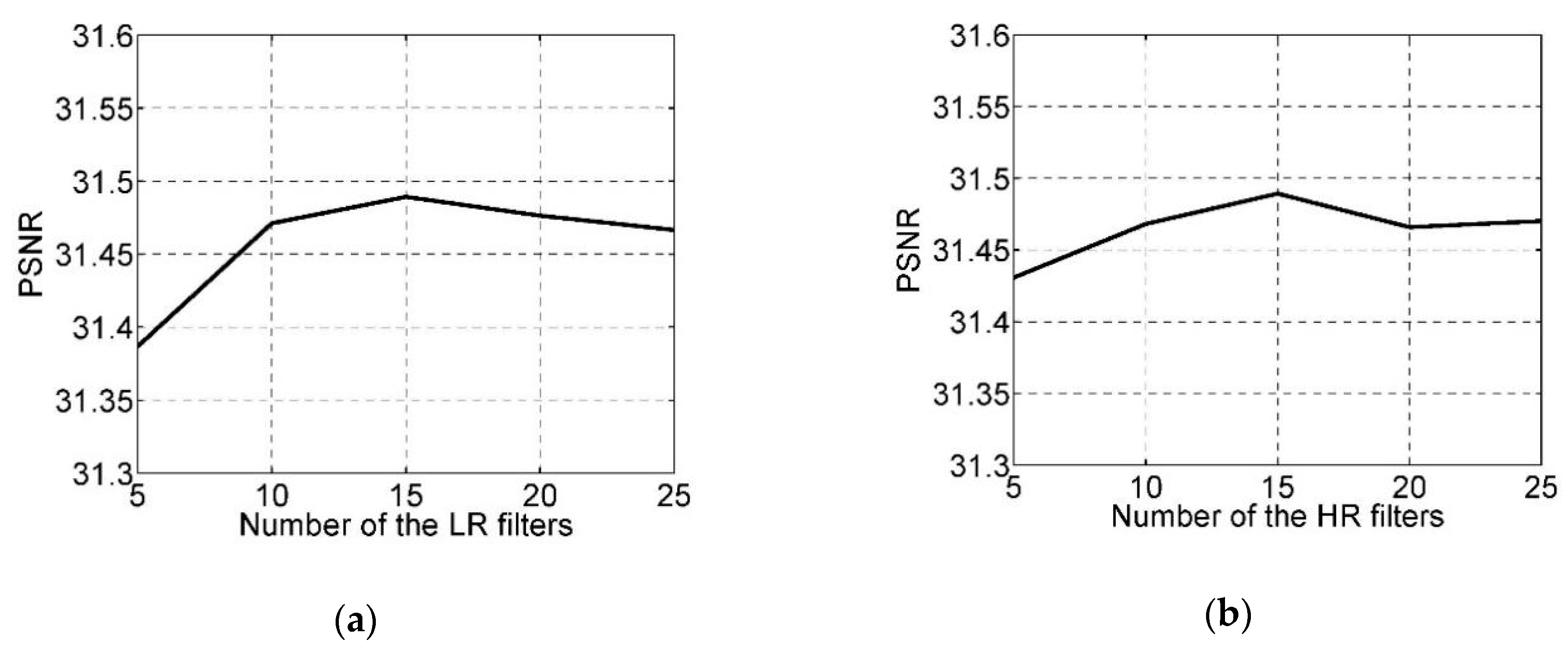
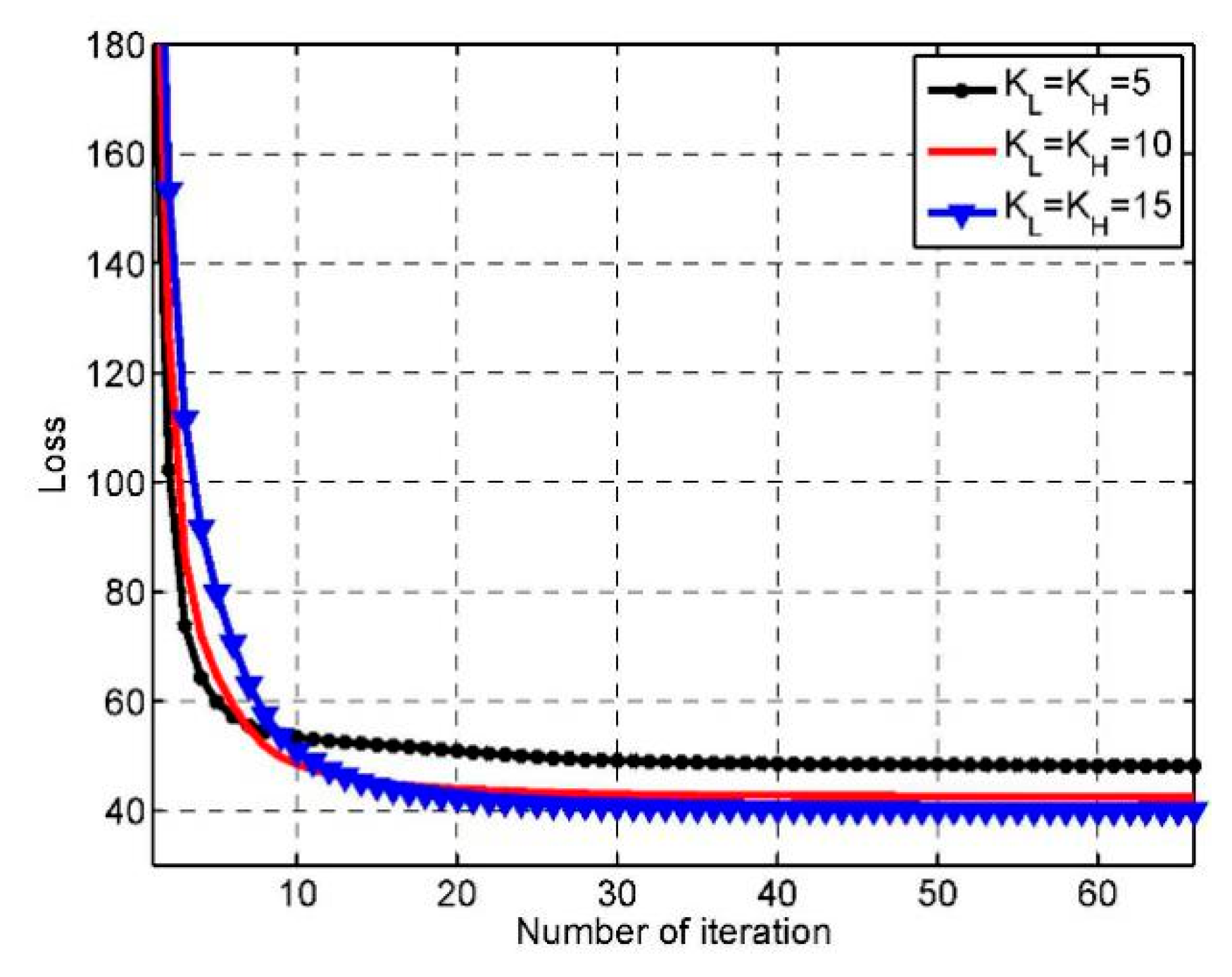
4.2.1. Number of Filters

In general, the more filters the better performance, because the more filters there are, the more feature types will be extracted, which leads to a strong ability of model expression. We adopted qualitative analysis to examine the impacts of the numbers of LR and HR filters $K_L$ and $K_H$. The sizes of the LR, HR, and mapping filters were set to $s_L=s_H=8,s_M=3$. We first fixed the number of the HR filters $K_H=15$, and varied the number of the LR filters from 5 to 25. For each number we trained a model on the training set and calculated the peak signal-to-noise ratio (PSNR) [56] averaged over the testing set. PSNR is a metric that has been widely used for evaluating image restoration quality quantitatively. Figure 3a depicts the PSNR curve with respect to $K_L$; we can see that the PSNR had some improvement with the increasing of $K_L$ for $K_L<15$. However, when $K_L>15$, the PSNR began to decline. We also made the same investigation on the number of HR filters. The $s_L$, $s_H$ and $s_M$ remained unchanged, and the $K_L$ was set to 15. We observed the model performance with $K_H$ varying from 5 to 25 as shown in Figure 3b. Overall, the PSNR had an obvious increase for $K_H<15$, but it dropped slightly when $K_H=15$. According to the above observation, the number of the LR and HR filters were set to $K_L=K_H=15$.

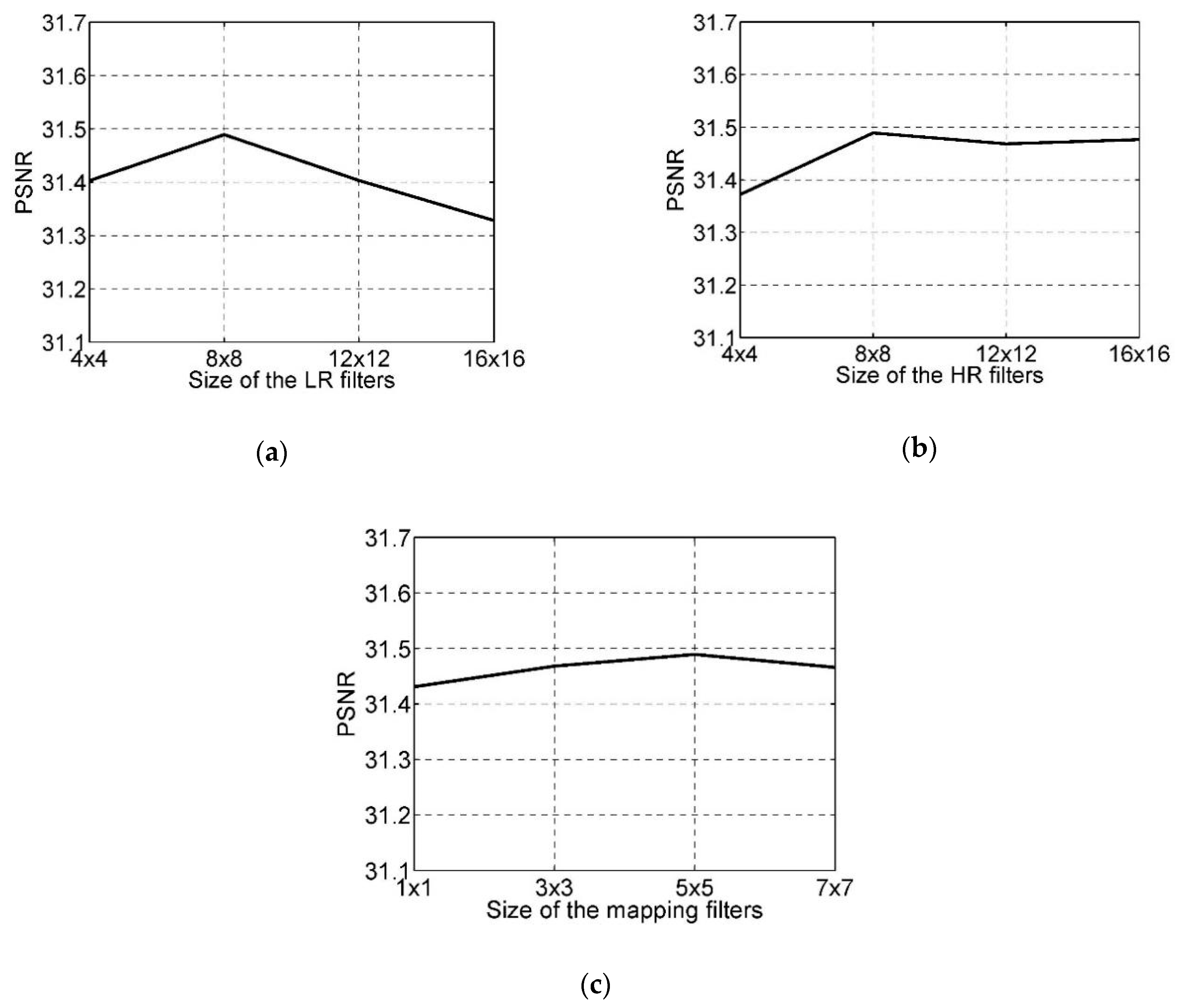
4.2.2. Size of Filters

In the proposed model there are three types of filters whose sizes all affect the model performance. Like the investigation of the filter number, we examined the impact of one type by fixing the other two types of filters. First, the $s_H,s_M$ were set to 8 and 3, respectively, and different $s_L$, ranging from $4$ to $16$ were tried. From Figure 4a we can see that the model achieved the best PSNR for $s_L=8$, while when $s_L>8$ the PSNR had a linear decline. For the largest size of $s_L$, the performance was the worst. Then, we observed the impact of the size of the HR filters on the model performance. The sizes of the LR and mapping filters were set to $s_L=8$ and $s_M=3$. The PSNR curve as a function of $s_H$ is depicted in Figure 4b. The results show that when $s_H=8$n the PSNR reached the top. Different from the LR filters, when $s_H>8$ the PSNR did not decrease linearly but rose again. Therefore, combining the observations of the LR and HR filters, we can demonstrate that it is not the larger the better; excessive enlargement of the filter size may cause the degradation of the performance.

At last, we turn to the size of the mapping filters which describe the relationship between the LR and HR feature maps. Intuitively, the larger $s_M$ is, the more neighborhood information the transformation process uses, at the same time, it is more robust to the outliers. On the other hand, larger filter size will weaken the representation of the central pixel. We fixed the sizes of LR and HR filters as $s_L=s_H=8$ and varied the size of the mapping filters to validate the above statement. Figure 4c shows the PSNR curve with varying $s_M$, we can see that the performance was the worst for $s_M=1$. That is because no neighborhood information was taken advantage of in the transformation, and each pixel in the HR feature maps was just related to the pixels on the same location in the LR feature maps. With the growth of the $s_M$, the performance improved. However, when the $s_M$ became intemperately large, the PSNR dropped again. Based on the above results and also in view of the running time, we set the parameters as $s_L=s_H=8$ and $s_M=3$ in later experiments.

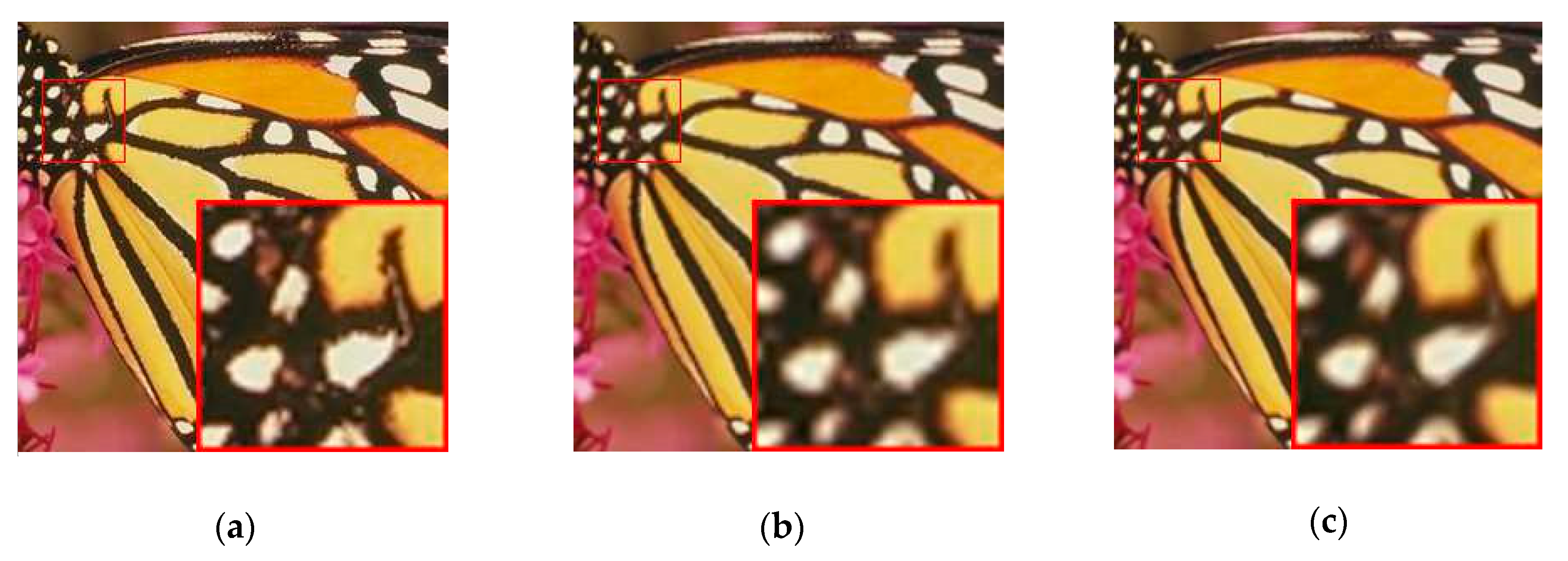
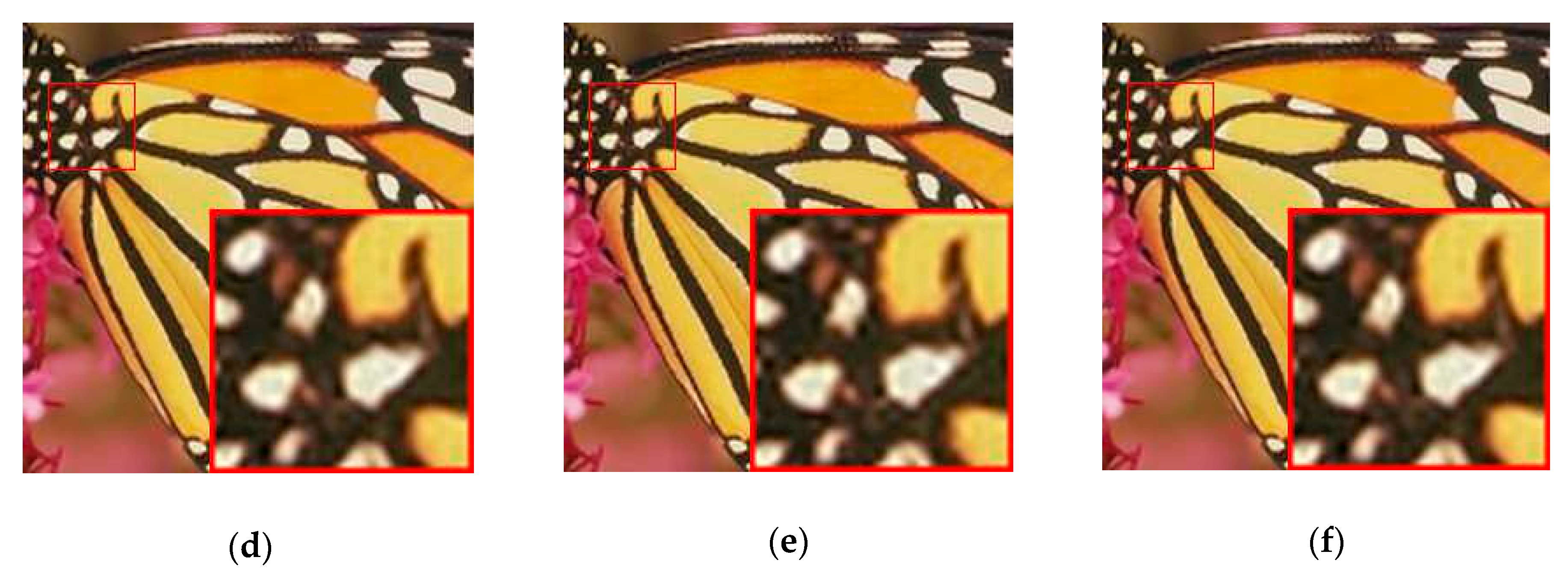
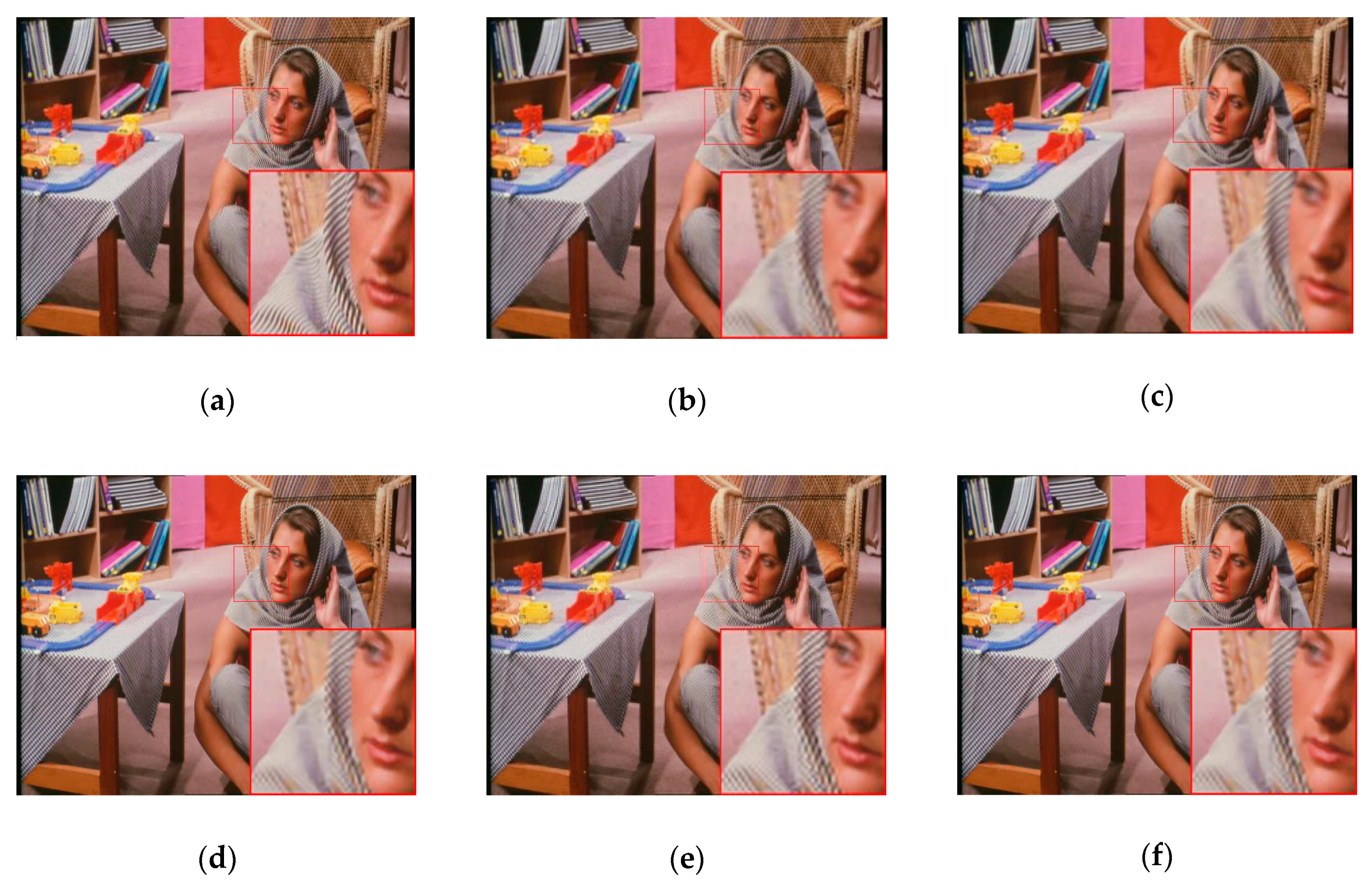
4.3. Super-Resolution Experiments

In order to validate the effectiveness of the proposed method, we compared it with four state-of-the-art methods on 15 commonly used images in the SR problem [57]. The methods include bicubic interpolation (BI), soft-decision-adaptive interpolation (SAI) [58], the conventional convolutional sparse coding (CSC) [24] method, and the linear mapping-based convolutional sparse coding (LMCSC) method [22], in which BI is a traditional interpolation method, SAI provides a powerful result in preserving edge structures for interpolation, while CSC can deal with the consistency issue. Note that, in comparison, the LMCSC is also trained in the full-size LR images instead of the down-sampled ones, so it does not need a zero-padding operation for the LR-HR linear transformation. Besides, all the convolutional methods adopted 15 LR and HR filters, and the filter sizes were all $8\times 8$.

Figure 5 depicts the filters learned by CSC, LMCSC and SCCSL, respectively, under the same condition. We can see that the LR and HR filters learned by CSC have similar structures due to strong coupling, which limits the diversity of the model. In contrast, LMCSC and SCCSL obtain much finer HR filters.

Two commonly used evaluating indices, PSNR and structural similarity index (SSIM) [59,60], were used in the comparison. SSIM is a measure of similarity between uncompressed undistorted image and distorted image which was proposed by the laboratory for image and video engineering at the university of Texas at Austin.

Table 1. The PSNR (dB) results of the 15 images by different methods, and bold font indicates that the algorithm has the best PSNR value on a single image.

Methods	Images
	Butterfly	Face	Bird	Comic	Woman	Foreman	Coast.	Flowers
BI	26.87	34.14	36.29	24.52	31.60	32.08	28.59	29.81
SAI	25.18	33.02	32.24	24.14	28.66	30.36	27.46	28.05
SCS	29.93	34.83	38.19	25.20	33.52	33.40	29.72	31.64
LMSCS	30.12	35.67	39.36	25.29	34.13	34.18	30.30	32.23
SCCSL	30.47	35.69	39.67	25.32	34.24	34.14	30.41	32.30
	Zebra	Lena	Bridge	Baby	Peppers	Man	Barbara	Avg. val.
BI	28.39	34.08	27.11	36.51	32.47	28.55	27.21	30.55
SAI	26.73	31.59	24.88	33.63	31.20	27.50	26.37	28.73
SCS	28.53	35.33	26.97	37.19	33.20	29.96	28.08	31.71
LMSCS	28.56	36.20	27.44	38.51	33.50	30.35	28.42	32.28
SCCSL	28.64	36.28	27.42	38.52	33.78	30.42	28.45	32.38

and

Table 2. The SSIM results of the 15 images by different methods, and bold font indicates that the algorithm has the best SSIM value on a single image.

Methods	Images
	Butterfly	Face	Bird	Comic	Woman	Foreman	Coast.	Flowers
BI	0.86	0.81	0.95	0.69	0.91	0.91	0.73	0.85
SAI	0.89	0.83	0.94	0.80	0.92	0.92	0.73	0.86
SCS	0.94	0.85	0.97	0.84	0.95	0.95	0.80	0.91
LMSCS	0.94	0.89	0.98	0.85	0.96	0.96	0.85	0.93
SCCSL	0.95	0.89	0.98	0.86	0.96	0.96	0.85	0.93
	Zebra	Lena	Bridge	Baby	Peppers	Man	Barbara	Avg. val.
BI	0.75	0.87	0.72	0.93	0.85	0.78	0.80	0.83
SAI	0.85	0.88	0.72	0.93	0.88	0.80	0.80	0.85
SCS	0.86	0.91	0.81	0.95	0.89	0.85	0.85	0.89
LMSCS	0.88	0.93	0.84	0.97	0.91	0.88	0.87	0.91
SCCSL	0.88	0.93	0.84	0.97	0.91	0.88	0.87	0.91

exhibit the PSNR and SSIM results of the 15 images by different methods. We can see that SCCSL outperformed others in most cases of the PSNR results, except that it is slightly worse than LMCSC for images Foreman and Bridge. In addition, as two baseline methods, BI and SAI were inferior to other three methods. The PSNR of SCCSL had a gain of about 0.1 dB and 0.7 dB compared with LMCSC and CSC, respectively. For the SSIM results, LMCSC and SCCSL are in the first echelon, and their values were nearly identical. The strong coupling method CSC is behind them, and BI is the worst.

Figure 6 and Figure 7 show the SR results of the images Butterfly and Barbara by different methods. The figures show that BI and SAI produce relatively blurry results, while other convolutional methods perform well in detail and have similar visual effects.

In a word, super-resolution experiments show that LR and HR filter learning are of great guiding significance for the design of deep learning network filter banks, which helps to maintain the spatial information of images and improve the reconstruction effect.

5. Discussions

5.1. Convergence

Since all the variables in the model are computed alternately during the training process, the loss easily gets stuck in the local minimum and behaves swinging. In order to validate the convergence of the algorithm, we examine the loss which is calculated via Equation (6) of each iteration in training phase. Figure 8 shows the loss curves of three models which use different filter numbers during the training. We have three observations: First, the algorithm has good convergence as all three curves tend to be stable after 30 iterations, and the curves are rather smooth. Second, the more filters the model uses, the slower the model converges. When $K_L=K_H=5$, the decreasing rate of the loss is obviously slowed down after five iterations. But this phenomenon occurs in the 10th and 15th iterations for $K_L=K_H=10$ and $K_L=K_H=15$, respectively. Finally, the more filters the model has, the higher accuracy the model achieves. When the number of filters rises from 5 to 10, the stable loss dropped by about 5.82. But this number becomes about 2.42 when the number of filters rises from 10 to 15. Even though the training accuracy increases with the growth of the filter number, this increased trend becomes obscure.

5.2. Time Complexity

Here we mainly consider the time complexity of the methods of the testing phase. The proposed method first calculates the LR feature maps via Equation (1), and then it computes the HR feature maps via Equation (27). At last it synthesizes the HR image via Equation (28). Among all formulas, the time complexity is dominated by the Equation (1) which can be solved in $\mathcal{O}\left(K_{L}MNlog\left(MN\right)\right)$ in the Fourier domain. In fact, CSC, LMCSC and SCCSL have the same time complexity, because SCCSL requires extra transformation operation, SCCSL is slightly slower than the other two methods.

Table 3. Time comparison of different methods.

Methods	BI	SAI	CSC	LMCSC	SCCSL
Time (sec)	0.01	0.07	4.14	4.23	4.31

gives the time comparison of different methods. BI and SAI have absolute advantages over the other three methods which are at the same level.

In summary, SCCSL can obtain better results of image super-resolution compared with BI, SAI, LMCSC and CSC, because the spatial information of images is maintained and the reconstruction effect is improved. Furthermore, in order to improve the image super-resolution accuracy, a small number of LR filters and a large number of HR filters are used for the HR image reconstruction process. However, the experiments show that the number of filters is not as large as possible. In addition, compared with other algorithms in this paper, the non-linear algorithm SCCSL takes more time in the testing phase. Since SCCSL converts transforms into Fourier domains under the ADMM framework, convolution operations are used to increase flexibility. Based on the convolution operations, neighborhoods within the filter size and the adjustable filter size, SCCSL is a more flexible and efficient approach for image super-resolution problem. Furthermore, SCCSL has room for improvement in time complexity.

6. Conclusions

We propose a novel semi-coupled convolutional sparse learning method of image super-resolution. It builds a convolutional mapping relationship between the LR and HR feature maps to weaken the strong coupling of the conventional CSC methods. The learned HR filters show good structure and fine details. Experiment results show that the proposed method performs better than several state-of-the-art methods in both numerical evaluating indices and visual effects. More importantly, the linear mapping-based model can be seen as a special case of SCCSL, which demonstrates the generalization of the proposed model.

References

1. Wright, J.; Ma, Y.; Mairal, J.; Sapiro, G.; Huang, T.S.; Yan, S. Sparse Representation for Computer Vision and Pattern Recognition. Proc. IEEE 2010, 98, 1031–1044. [Google Scholar] [CrossRef]
2. Donoho, D.L. Compressed sensing. IEEE Trans. Inform. Theory 2006, 52, 1289–1306. [Google Scholar] [CrossRef]
3. Candès, E.J.; Romberg, J.K.; Tao, T. Robust uncertainty principles: Exact signal reconstruction from highly incomplete frequency information. IEEE Trans. Inform. Theory 2006, 52, 489–509. [Google Scholar] [CrossRef]
4. Gan, L. Block Compressed Sensing of Natural Images. In Proceedings of the 2007 IEEE 15th International Conference on Digital Signal Processing, Assam, India, 18–21 December 2007; pp. 403–406. [Google Scholar]
5. Fu, Y.; Gao, J.; Tien, D.; Lin, Z.; Hong, X. Tensor LRR and Sparse Coding-Based Subspace Clustering. IEEE Trans. Neural Netw. Learn. Syst. 2017, 27, 2120–2133. [Google Scholar] [CrossRef] [PubMed]
6. Zeiler, M.D.; Krishnan, D.; Taylor, G.W.; Fergus, R. Deconvolutional networks. In Proceedings of the Twenty-Third IEEE Conference Computer Vision Pattern Recognition, San Francisco, CA, USA, 13–18 June 2010; pp. 2528–2535. [Google Scholar]
7. Papyan, V.; Sulam, J.; Elad, M. Working Locally Thinking Globally: Theoretical Guarantees for Convolutional Sparse Coding. IEEE Trans. Signal Process. 2017, 65, 5687–5701. [Google Scholar] [CrossRef]
8. Wang, J.; Wang, Z.; Tao, D.; See, S.; Wang, G. Learning Common and Specific Features for RGB-D Semantic Segmentation with Deconvolutional Networks. In Proceedings of the European Conference on Computer Vision ECCV, Amsterdam, The Netherlands, 8–16 October 2016; pp. 664–679. [Google Scholar]
9. Dandois, J.P. Remote Sensing of Vegetation Structure Using Computer Vision. Remote Sens. 2010, 2, 1157–1176. [Google Scholar] [CrossRef] [Green Version]
10. Zeiler, M.D.; Taylor, G.W.; Fergus, R. Adaptive deconvolutional networks for mid and high level feature learning. In Proceedings of the IEEE International Conference Computer Vision ICCV, Barcelona, Spain, 6–13 November 2011; pp. 2018–2025. [Google Scholar]
11. Nekrasov, V.; Ju, J.; Choi, J.; Nekrasov, V.; Ju, J.; Choi, J.; Nekrasov, V.; Ju, J.; Choi, J. Global Deconvolutional Networks for Semantic Segmentation. arXiv 2016, arXiv:1602.03930. [Google Scholar] [Green Version]
12. Kim, K.I.; Kwon, Y. Single-Image Super-Resolution Using Sparse Regression and Natural Image Prior. IEEE Trans. Pattern Anal. Mach. Intell. 2010, 32, 1127–1133. [Google Scholar]
13. Yang, J.; Wright, J.; Huang, T.S.; Ma, Y. Image Super-Resolution Via Sparse Representation. IEEE Trans. Image Process. 2010, 19, 2861–2873. [Google Scholar] [CrossRef]
14. Wang, S.; Yue, B.; Liang, X.; Jiao, L. How Does the Low-Rank Matrix Decomposition Help Internal and External Learnings for Super-Resolution. IEEE Trans. Image Process. 2017, 27, 1086–1099. [Google Scholar] [CrossRef] [Green Version]
15. Mei, S.; Xin, Y.; Ji, J.; Zhang, Y.; Shuai, W.; Qian, D. Hyperspectral Image Spatial Super-Resolution via 3D Full Convolutional Neural Network. Remote Sens. 2017, 9, 1139. [Google Scholar] [CrossRef]
16. Dong, W.; Fu, F.; Shi, G.; Cao, X.; Wu, J.; Li, G.; Li, G. Hyperspectral Image Super-Resolution via Non-Negative Structured Sparse Representation. IEEE Trans. Image Process. 2016, 25, 2337–2352. [Google Scholar] [CrossRef] [PubMed]
17. Yue, B.; Wang, S.; Liang, X.; Jiao, L. Robust Noisy Image Super-Resolution Using l1-norm Regularization and Non-local Constraint. In Proceedings of the 13th Asian Conference on Computer Vision ACCV, Taipei, Taiwan, 20–24 November 2016; pp. 34–49. [Google Scholar]
18. Hou, B.; Zhou, K.; Jiao, L. Adaptive Super-Resolution for Remote Sensing Images Based on Sparse Representation with Global Joint Dictionary Model. IEEE Trans. Geosci. Remote Sens. 2017, 56, 2312–2327. [Google Scholar] [CrossRef]
19. Liu, J.; Gong, M.; Qin, K.; Zhang, P. A Deep Convolutional Coupling Network for Change Detection Based on Heterogeneous Optical and Radar Images. IEEE Trans. Neural Netw. Learn. Syst. 2016, 29, 545–559. [Google Scholar] [CrossRef]
20. Wei, J.; Wang, L.; Liu, P.; Song, W. Spatiotemporal Fusion of Remote Sensing Images with Structural Sparsity and Semi-Coupled Dictionary Learning. Remote Sens. 2016, 9, 21. [Google Scholar] [CrossRef]
21. Osendorfer, C.; Soyer, H.; Smagt, P.V.D. Image Super-Resolution with Fast Approximate Convolutional Sparse Coding. In Proceedings of the International Conference on Neural Information Processing ICONIP, Kuching, Malaysia, 3–6 November 2014; Springer: Cham, Switzerland, 2014; pp. 250–257. [Google Scholar]
22. Gu, S.; Zuo, W.; Xie, Q.; Meng, D.; Feng, X.; Zhang, L. Convolutional Sparse Coding for Image Super-Resolution. In Proceedings of the IEEE International Conference on Computer Vision, Santiago, Chile, 7–13 December 2015; pp. 1823–1831. [Google Scholar]
23. Wang, S.; Zhang, L.; Liang, Y.; Pan, Q. Semi-coupled dictionary learning with applications to image super-resolution and photo-sketch synthesis. In Proceedings of the IEEE Conference Computer Vision Pattern Recognition, Providence, RI, USA, 16–21 June 2012; pp. 2216–2223. [Google Scholar]
24. Bristow, H.; Eriksson, A.; Lucey, S. Fast Convolutional Sparse Coding. In Proceedings of the IEEE Conference Computer Vision and Pattern Recognition, Portland, OR, USA, 23–28 June 2013; pp. 391–398. [Google Scholar]
25. Heide, F.; Heidrich, W.; Wetzstein, G. Fast and flexible convolutional sparse coding. In Proceedings of the IEEE Conference Computer Vision and Pattern Recognition, Boston, MA, USA, 7–12 June 2015; pp. 5135–5143. [Google Scholar]
26. Wohlberg, B. Efficient Algorithms for Convolutional Sparse Representations. IEEE Trans. Image Process. 2016, 25, 301–315. [Google Scholar] [CrossRef]
27. Boyd, S.; Parikh, N.; Chu, E.; Peleato, B.; Eckstein, J. Distributed Optimization and Statistical Learning via the Alternating Direction Method of Multipliers. Found. Trends Mach. Learn. 2010, 3, 1–122. [Google Scholar] [CrossRef]
28. Lu, C.; Feng, J.; Yan, S.; Lin, Z. A Unified Alternating Direction Method of Multipliers by Majorization Minimization. IEEE Trans. Pattern Anal. Mach. Intell. 2018, 40, 527–541. [Google Scholar] [CrossRef]
29. Mairal, J.; Elad, M.; Sapiro, G. Sparse Representation for Color Image Restoration. IEEE Trans. Image Process. 2008, 17, 53–69. [Google Scholar] [CrossRef]
30. Wright, J.; Yang, A.Y.; Ganesh, A.; Sastry, S.S.; Ma, Y. Robust Face Recognition via Sparse Representation. IEEE Trans. Pattern Anal. Mach. Intell. 2009, 31, 210–227. [Google Scholar] [CrossRef]
31. Wang, J.; Lu, C.; Wang, M.; Li, P.; Yan, S.; Hu, X. Robust face recognition via adaptive sparse representation. IEEE Trans. Cybern 2014, 44, 2368–2378. [Google Scholar] [CrossRef] [PubMed]
32. Agarwal, S.; Roth, D. Learning a Sparse Representation for Object Detection. In Proceedings of the European Conference Computer Vision ECCV, Copenhagen, Denmark, 28–31 May 2002; pp. 113–130. [Google Scholar]
33. Ren, X.; Ramanan, D. Histograms of Sparse Codes for Object Detection. In Proceedings of the IEEE Conference on Computer Vision & Pattern Recognition CVPR, Portland, OR, USA, 23–28 June 2013. [Google Scholar]
34. Gu, J.; Jiao, L.; Yang, S.; Liu, F. Fuzzy Double C-Means Clustering Based on Sparse Self-Representation. IEEE Trans. Fuzzy Syst. 2017, 26, 612–626. [Google Scholar] [CrossRef]
35. Shi, J.; Jiang, Z.; Feng, H.; Ma, Y. Sparse coding-based topic model for remote sensing image segmentation. In Proceedings of the 2013 IEEE International Geoscience and Remote Sensing Symposium—IGARSS, Melbourne, Australia, 21–26 July 2013. [Google Scholar]
36. Xue, Z.; Du, P.; Su, H.; Zhou, S. Discriminative Sparse Representation for Hyperspectral Image Classification: A Semi-Supervised Perspective. Remote Sens. 2017, 9, 386. [Google Scholar] [CrossRef]
37. Liu, J.; Wu, Z.; Wei, Z.; Liang, X.; Le, S. Spatial-Spectral Kernel Sparse Representation for Hyperspectral Image Classification. IEEE J. Sel. Top. Appl. Earth Obs. Remote Sens. 2013, 6, 2462–2471. [Google Scholar] [CrossRef]
38. Rida, I.; Al-Maadeed, N.; Al-Maadeed, S.; Bakshi, S. A comprehensive overview of feature representation for biometric recognition. Multimed. Tools Appl. 2018, 1–24. [Google Scholar] [CrossRef]
39. Congzhong, W.U.; Changsheng, H.U.; Zhang, M.; Xie, Z.; Zhan, S. Single Image Super-resolution Reconstruction via Supervised Multi-dictionary Learning. Opto Electron. Eng. 2016, 43, 69–75. [Google Scholar]
40. Rida, I.; Herault, R.; Gasso, G. An efficient supervised dictionary learning method for audio signal recognition. arXiv 2018, arXiv:1812.04748. [Google Scholar]
41. Singhal, V.; Majumdar, A. Supervised Deep Dictionary Learning for Single Label and Multi-Label Classification. In Proceedings of the 2018 International Joint Conference on Neural Networks (IJCNN), Rio de Janeiro, Brazil, 8–13 July 2018; pp. 2161–4407. [Google Scholar]
42. Huang, Y.; Liu, X.; Xiang, T.; Fan, Z.; Chen, Y.; Jiang, R. Deep supervised dictionary learning for no-reference image quality assessment. J. Electron. Imaging 2018, 27, 1. [Google Scholar] [CrossRef]
43. Jiao, L.; Zhang, S.; Li, L.; Yang, S.; Liu, F.; Hao, H.; Dong, H. A Novel Image Representation Framework Based on Gaussian Model and Evolutionary Optimization. IEEE Trans. Evol. Comput. 2017, 21, 265–280. [Google Scholar] [CrossRef]
44. Jiao, L.; Liang, M.; Chen, H.; Yang, S.; Liu, H.; Cao, X. Deep Fully Convolutional Network-Based Spatial Distribution Prediction for Hyperspectral Image Classification. IEEE Trans. Geosci. Remote Sens. 2017, 55, 5585–5599. [Google Scholar] [CrossRef]
45. Lecun, Y.; Boser, B.; Denker, J.S.; Henderson, D.; Howard, R.E.; Hubbard, W.; Jackel, L.D. Backpropagation Applied to Handwritten Zip Code Recognition. Neural Comput. 2014, 1, 541–551. [Google Scholar] [CrossRef]
46. Krizhevsky, A.; Sutskever, I.; Hinton, G.E. ImageNet Classification with Deep Convolutional Neural Networks. In Proceedings of the International Conference on Neural Information Processing Systems, NIPS, Lake Tahoe, CA, USA, 3–6 December 2012; pp. 1106–1114. [Google Scholar]
47. Jiao, L.; Zhang, S.; Li, L.; Liu, F.; Ma, W. A modified convolutional neural network for face sketch synthesis. Pattern Recognit. 2017, 76, 125–136. [Google Scholar] [CrossRef]
48. Feng, J.; Wang, L.; Yu, H.; Jiao, L.; Zhang, X. Divide-and-Conquer Dual-Architecture Convolutional Neural Network for Classification of Hyperspectral Images. Remote Sens. 2019, 11, 484. [Google Scholar] [CrossRef]
49. Li, Y.; Wang, Y.; Li, Y.; Jiao, L.; Zhang, X.; Stolkin, R. Single image super-resolution reconstruction based on genetic algorithm and regularization prior model. Inf. Sci. Int. J. 2016, 372, 196–207. [Google Scholar] [CrossRef] [Green Version]
50. Yang, S.; Liu, Z.; Wang, M.; Sun, F.; Jiao, L. Multitask dictionary learning and sparse representation based single-image super-resolution reconstruction. Neurocomputing 2011, 74, 3193–3203. [Google Scholar] [CrossRef]
51. Bianco, S.; Cusano, C.; Schettini, R. Single and Multiple Illuminant Estimation Using Convolutional Neural Networks. IEEE Trans. Image Process. 2017, 26, 4347–4362. [Google Scholar] [CrossRef] [PubMed]
52. Zhong, W.; Kwok, J.T. Fast Stochastic Alternating Direction Method of Multipliers. In Proceedings of the International Conference on Machine Learning ICML, Beijing, China, 21–26 June 2014; pp. 46–54. [Google Scholar]
53. Dong, C.; Loy, C.C.; He, K.; Tang, X. Learning a Deep Convolutional Network for Image Super-Resolution. In Proceedings of the European Conference Computer Vision, Zurich, Switzerland, 6–12 September 2014; pp. 184–199. [Google Scholar]
54. Yoon, Y.; Jeon, H.; Yoo, D.; Lee, J.; Kweon, I.S. Learning a Deep Convolutional Network for Light-Field Image Super-Resolution. In Proceedings of the IEEE International Conference Computer Vision Workshops, Santiago, Chile, 7–13 December 2015; pp. 57–65. [Google Scholar]
55. Yu, G.; Sapiro, G.; Mallat, S. Solving Inverse Problems with Piecewise Linear Estimators: From Gaussian Mixture Models to Structured Sparsity. IEEE Trans. Image Process. 2012, 21, 2481–2499. [Google Scholar]
56. Bo, L.; Rui, Y.; Jiang, H. Remote-Sensing Image Compression Using Two-Dimensional Oriented Wavelet Transform. IEEE Trans. Geosci. Remote Sens. 2010, 49, 236–250. [Google Scholar]
57. Dong, C.; Loy, C.C.; He, K.; Tang, X. Image Super-Resolution Using Deep Convolutional Networks. IEEE Trans. Pattern Anal. Mach. Intell. 2016, 38, 295–307. [Google Scholar] [CrossRef]
58. Zhang, X.; Wu, X. Image Interpolation by Adaptive 2-D Autoregressive Modeling and Soft-Decision Estimation. IEEE Trans. Image Process. 2008, 17, 887–896. [Google Scholar] [CrossRef]
59. Wang, Z.; Bovik, A.C.; Sheikh, H.R.; Simoncelli, E.P. Image quality assessment: From error visibility to structural similarity. IEEE Trans. Image Process. 2004, 13, 600–612. [Google Scholar] [CrossRef] [PubMed]
60. Pan, Z.; Jing, Y.; Huang, H.; Hu, S.; Sun, W. Super-Resolution Based on Compressive Sensing and Structural Self-Similarity for Remote Sensing Images. IEEE Trans. Geosci. Remote Sens. 2013, 51, 4864–4876. [Google Scholar] [CrossRef]
Figure 1. The framework of convolutional sparse coding (CSC).
Remotesensing 11 02593 g001
Figure 2. The relationship between convolutional and linear mapping functions. (a) Convolutional mapping architecture. (b) Linear mapping architecture.
Remotesensing 11 02593 g002
Figure 3. The impacts of the number of the filters. (a) K L . (b) K H .
Remotesensing 11 02593 g003
Figure 4. The impacts of the size of the filters. (a) s L . (b) s H . (c) s M .
Remotesensing 11 02593 g004
Figure 5. Filters learned by different methods. (a) Filters learned by conventional convolutional sparse coding (CSC). (b) Filters learned by linear mapping-based convolutional sparse coding (LMCSC). (c) Filters learned by semi-coupled convolutional sparse learning (SCCSL).
Remotesensing 11 02593 g005
Figure 6. SR results of the image Butterfly by different methods. (a) Original image. (b) Bicubic interpolation (BI). (c) Soft-decision-adaptive interpolation (SAI). (d) CSC. (e) LMCSC. (f) SCCSL.
Remotesensing 11 02593 g006aRemotesensing 11 02593 g006b
Figure 7. SR results of the image Barbara by different methods. (a) Original image. (b) BI. (c) SAI. (d) CSC. (e) LMCSC. (f) SCCSL.
Remotesensing 11 02593 g007
Figure 8. The convergence of the proposed algorithm.
Remotesensing 11 02593 g008