Article

InSAR Time Series Analysis of L-Band Data for Understanding Tropical Peatland Degradation and Restoration

1
State Key Laboratory of Geodesy and Earth’s Dynamics, Institute of Geodesy and Geophysics, Chinese Academy of Sciences, Wuhan 430077, China
2
School of Geographical and Earth Sciences, University of Glasgow, Glasgow G12 8QQ, UK
3
COMET, School of Engineering, Newcastle University, Newcastle Upon Tyne NE1 7RU, UK
4
Geological Survey of Japan, National Institute of Advanced Industrial Science and Technology, Tsukuba 305-8567, Japan
*
Author to whom correspondence should be addressed.
Remote Sens. 2019, 11(21), 2592; https://doi.org/10.3390/rs11212592
Submission received: 8 September 2019 / Revised: 31 October 2019 / Accepted: 31 October 2019 / Published: 5 November 2019
(This article belongs to the Special Issue Remote Sensing of Peatlands II)

Abstract

:
In this study, satellite radar observations are employed to reveal spatiotemporal changes in ground surface height of peatlands that have, and have not, undergone restoration in Central Kalimantan, Indonesia. Our time series analysis of 26 scenes of Advanced Land Observation Satellite-1 (ALOS-1) Phased-Array L-band Synthetic-Aperture Radar (PALSAR) images acquired between 2006 and 2010 suggests that peatland restoration was positively affected by the construction time of dams—the earlier the dam was constructed, the more significant the restoration appears. The results also suggest that the dams resulted in an increase of ground water level, which in turn stopped peat losing height. For peatland areas without restoration, the peatland continuously lost peat height by up to 7.7 cm/yr. InSAR-derived peat height changes allow the investigation of restoration effects over a wide area and can also be used to indirectly assess the relative magnitude and spatial pattern of peatland damage caused by drainage and fires. Such an assessment can provide key information for guiding future restoration activities.

Graphical Abstract

1. Introduction

As one of the most important natural wetland ecosystems in the world, peatlands cover about 2–3% of the Earth’s land surface and store 500 to 700 Gt of carbon [1], nearly equal to the atmospheric carbon pool (750 Gt) [2]. Therefore, peatlands play an important role in the global carbon cycle [3,4]. In the tropics, peatlands cover around 40 million hectares (Mha) and accumulate around 90 Gt of carbon, while more than 54% and 76% of this tropical peatland area and carbon storage occur in South-East Asia [5]. Although tropical peatlands are rich in carbon storage, land use changes, drainage, and recurrent fires have resulted in extensive peatland degradation in this region during the past 20 years [6,7]. From 1990 to 2010, the forest coverage of South-East Asia decreased from 268 million ha to 236 million ha (an average net loss of 1.6 million ha yr−1, 0.6% yr−1) [8], which results in a warmer, drier environment at local scale [9]. Drainage of peatlands causes peat oxidation and releases carbon into the atmosphere as CO2, which results in peat subsidence [10]. It is estimated that an additional drainage depth of 10 cm results in 0.9 cm peat subsidence and approximately 9 t CO2 ha−1yr−1 emissions [11]. Another severe consequence of drainage is that peat becomes dry and susceptible to fires during dry seasons (typically from June to October). Fires are the most severe in long dry seasons, such as the 1997/98 El Niño Southern Oscillation (ENSO) event. It was reported that 0.12–0.15 Gt of carbon was emitted due to peat combustion from Central Kalimantan, Indonesia during the ENSO dry season of 1997 [12]. The total carbon released to atmosphere due to the above emission from peat combustion in Indonesia in 1997 was between 0.81 and 2.57 Gt, which is equivalent to 13–40% of the mean annual global carbon emission from fossil fuels of 2001 [12]. Therefore, the restoration of peat hydrology and conservation of tropical peatlands is critical in order to prevent peat oxidation, peat fires and mitigate excess CO2 emission [13,14,15]. For example, from 2004 to 2008, hydrological restoration commenced in Central Kalimantan (of the Mega-Rice project drained landscape) by building large dams [15,16], and understanding the effectiveness of the restoration activity is important for guiding future restoration activities.
Interferometric Synthetic Aperture Radar (InSAR) measures surface displacements in the line of sight to the satellite by differencing the phase measurements between two complex radar images acquired at two epochs but with similar satellite geometries, and the resulting difference phase forms a new kind of image called an interferogram [17]. In the last two decades, InSAR has been proven to be a powerful tool for measuring the Earth’s surface movements [18]. It can be accurate to a few millimeters, with high spatial resolution (pixels in the order of sub-meters to tens of meters) over a wide area (e.g., 100 km × 100 km or even wider) [19].
The potential of InSAR to measure peat height changes has been explored [20,21,22,23,24,25,26,27]. For example, in 2011, using four scenes of European Remote Sensing (ERS, C-band) tandem pairs (1 day interval) from October 1997 to January 2000 and the four-pass (four SAR images) InSAR method, a subsidence rate of 2 cm/year was estimated for Central Kalimantan, Indonesia [21]. In another study, using two pairs of Sentinel-1A image, the first pair acquired in June 2015 and June 2016, and second pair in June 2016 and July 2017, subsidence and uplift signals are revealed by two-pass InSAR (D-InSAR) method in peatland of Pelalawan Regency, Riau, Indonesia [27]. The four-pass InSAR method only uses one pair of SAR images to detect the surface deformation; the other pair is used to generate topography information and then applied to remove the topographic phase contained in the first pair. Although C-band tandem pairs promise high coherence in tropic forest, coherence is low for a longer image acquisition interval (such as 35 days) in areas with high dense vegetation [28]. The temporal decorrelation likely makes it difficult to apply C-band SAR images in tropical peatlands area, comparison to L-band SAR images [28]. Because shorter wavelength (C-band) has weaker penetration capability than longer wavelength (L-band). This leads to C-band radar signals are primary reflected back from the tree canopy and only a few signals are returned from the trunk, while the situation is on the contrary for L-band. For both four-pass and two-pass InSAR method, the surface movement rate estimation is likely to be limited as well, because atmospheric effects, orbital ramps, and decorrelation effects are not mitigated by the methods [17]. In addition, no information on the surface movement history can be obtained as well.
To reduce the temporal decorrelation and various errors, InSAR time series algorithms are developed by using multitemporal SAR images since 2001, such as Permanent Scatterer InSAR (PSInSARTM) [29], Small BAseline Subset (SBAS) [30], SqueenSARTM [31]. For more details about the concept and procedure, please refer to Batuhan et al., [18], the paper provides good reviews on InSAR time series method. Different InSAR time series methods and datasets are applied in measuring peatlands surface change. Using Intermittent Small Baseline Subset (ISBAS) DInSAR algorithm, ERS C-band images (1992–2000) and Sentinel-1 C-band (2015–2016), Alshammari et al., [25] detected subsidence and uplift change over peatland areas in the northeast of Scotland, UK. Using 161 Sentinel-1 SAR (C-band) images and ISBAS method, Marshall et al., [24] also measured the deformation patterns of tropical peat swamp around Kuala Lumpur International Airport. Fiaschi et al., [32] detected uplift signal of up to 8.9 mm/year and subsidence signal of up to −11.6 mm/year in Irish peatlands by using 124 Sentinel-1A/B images acquired from 4 May 2015 to 1 March 2018 and PS-InSAR method. Although, C-band shows potential in measuring peatlands surface motion, it is likely hard to extract sufficient number of PS points and provide good coverage, particularly over a tropical peatlands area [24].
So far, the application of L-band data and InSAR time series methods for understanding peatlands degradation and restoration in tropical zone is rarely documented in peer-reviewed scientific literature. Therefore, the main goal of this study was to employ ALOS-1 PALSAR L-band SAR images (free of charge) acquired between 2006 and 2010, and InSAR Time Series with Atmospheric Estimation Model (InSAR TS+AEM) method to investigate the spatial and temporal evolution of the peatland surface change in Central Kalimantan, Indonesia. Since latest ALOS-2 PALSAR data are commercial data (~2200 USD for a standard archived Stripmap image), it restricts their use to many end users because of budget constraints. And then assess the effects of hydrological peatland restoration through the use of dams in the drainage systems, which is important knowledge for the planning of future restoration projects.

2. Materials and Methods
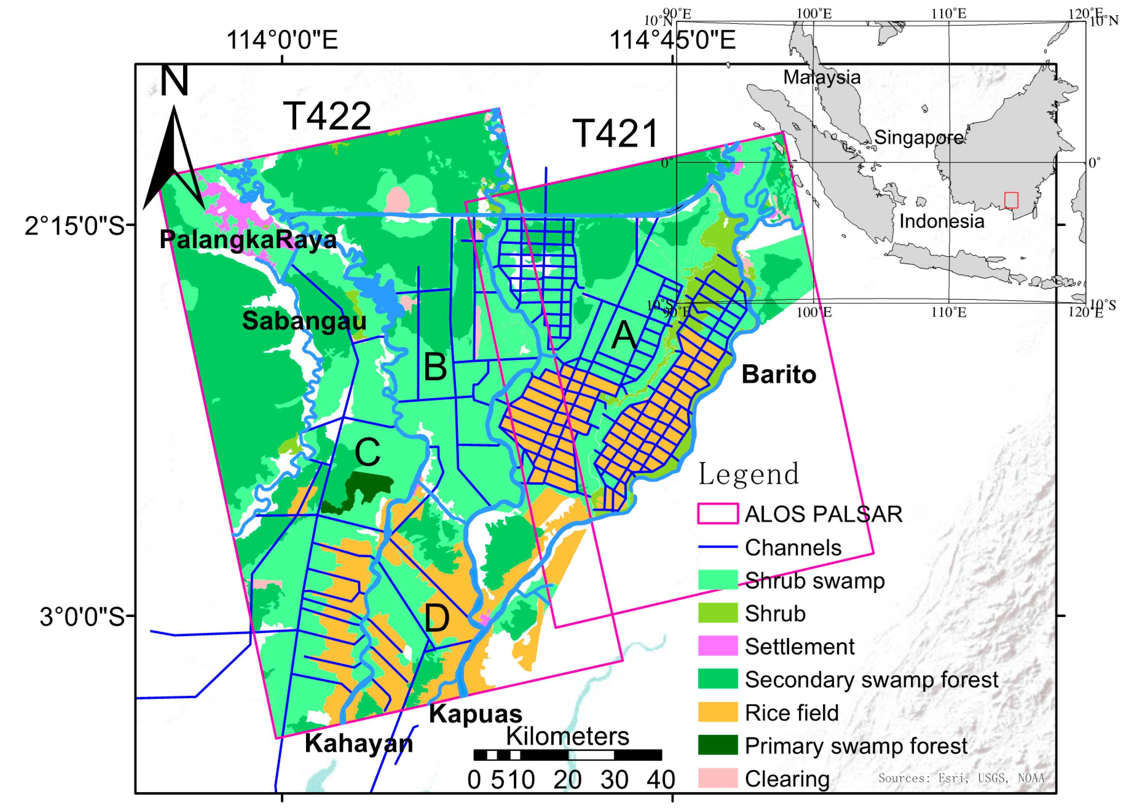
2.1. The Study Area

In 1996, the Indonesian Government initiated the One Million Hectare Mega Rice Project (MRP) in Central Kalimantan (Indonesia). The principal objective of the MRP was food (rice) production in the area between the Sabangau River in the west, the Kahayan and Kapuas Rivers in the south and the Barito River in the east (Figure 1). The area was divided into four blocks (A, B, C, and D) according to the rivers’ boundaries (light blue curves) in the MRP project, and the city of Palangkaraya is located in the north of Block C [16]. Large-scale deforestation was initiated in January 1996 to prepare the land for rice paddies, which involved mostly clear-felling the peat swamp forest and evacuating a massive network of in excess of 4400 km of drainage channels across the deep peat domes; some drainage channels were up to 30 m wide and 10 m deep [15,16,33].
In July 1999, the MRP was closed down because the area had been over-drained by the channels and unable to store water needed for agriculture irrigation. Consequently, the area was largely abandoned and is currently ‘unproductive’ and susceptible to flooding [35]. The drainage of the peatland caused by the network of extensive channels results in peat oxidation, subsidence, and regular outbreaks of large-scale fires [13,35,36]. Seven types of land cover dominate this area (Figure 1), i.e., shrub swamp, shrub, settlement, secondary swamp forest, rice field, primary swamp forest and clearing [34]. Most of the shrub swamp and rice field areas can be characterized as destroyed, abandoned and/or fire-damaged, and only a small part of the rice field area is still in use [14]. Note that the land cover data shown in Figure 1 was released in 2009 and an assumption was made in this study that there was no obvious land use change over the satellite observation period of 2006–2010.
In July 2004, hydrological restoration commenced in Block A under the CCFPI (Climate Change Forests and Peatlands in Indonesia) project, with the construction of five large drainage channel dams; 19 additional drainage channel dams were built in this area between 2007 and 2008, funded by the Central Kalimantan Peatland Project (CKPP). Between June and September 2005, seven dams were constructed in Block C within the framework of the Academy of Finland funded KEYTROP (Keys for Securing Tropical Peat Carbon) and the EU-funded RESTORPEAT (Restoration of Tropical Peatland for Sustainable Management of Renewable Natural Resources) projects [15,16]. The dams in Block A are similar to those in Block C in terms of size and design [15,16,37].

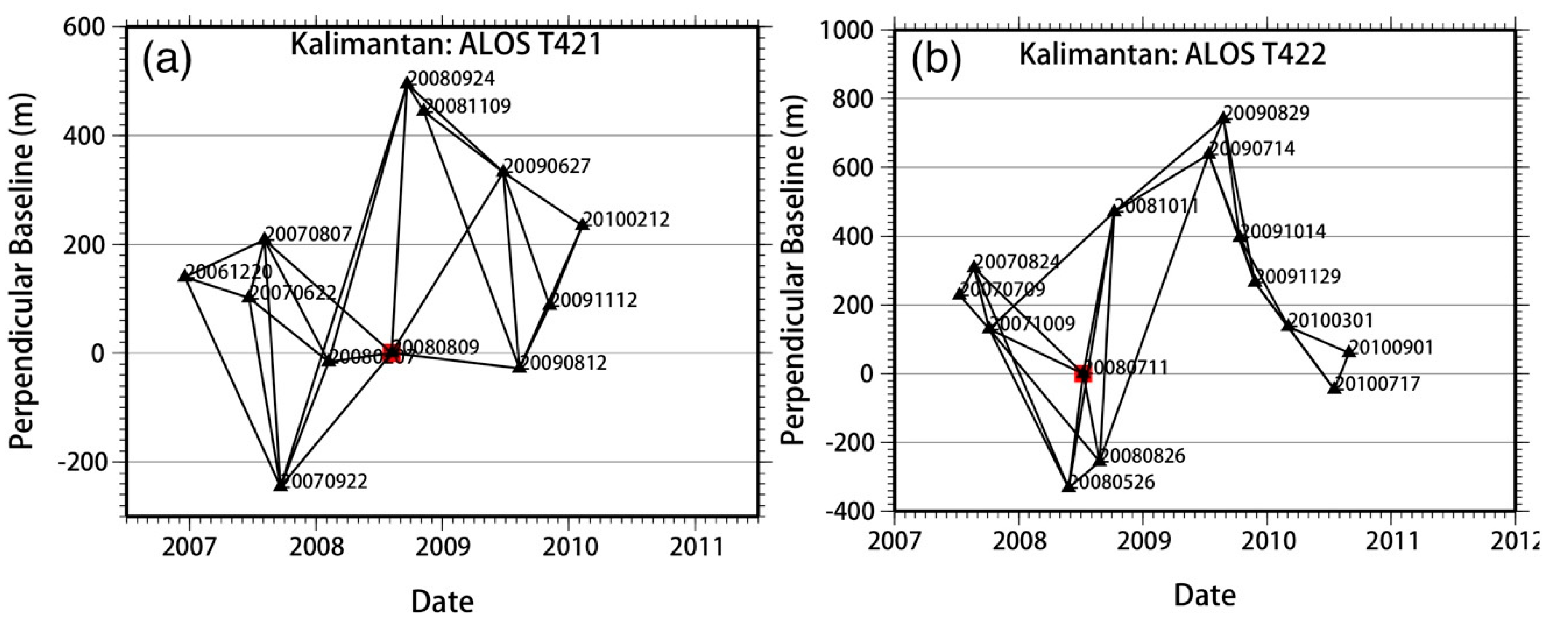
2.2. InSAR Interferometric Processing and Time Series Analysis

In this study, two adjacent tracks of L-band (a wavelength of 23.6 cm) ALOS-1 PALSAR images acquired between 2006 and 2010 were processed and analyzed (Table 1), covering a total area of 11,780 km2. L-band was used as this has a better penetration capability than shorter wavelength signals (such as C-band), and the ground and the trunks contribute to the signal and to avoid decorrelation caused by changes on the canopy. In this study, the coherence in heavy forest is generally low for interferograms with a perpendicular baseline (satellite separation) greater than 1000 m and/or a temporal baseline (i.e., time interval) longer than 1 year. To minimize the temporal decorrelation effects, only those image pairs with small baselines (i.e., perpendicular baseline < 1000 m and temporal baseline < 1 year) were selected for interferometric processing and further analysis (Figure 2). All the interferograms were formed from raw radar images using the JPL/Caltech ROI_PAC (Version 3.1b) [38] with multi-look factor of 8 (in range direction) by 16 (in azimuth direction) to reduce the speckle noise, with a final resolution of about 80 m by 80 m. The 3-arcsecond (about 90 m resolution) SRTM digital elevation model (DEM) [39] was used to remove topographic phase contribution. The interferograms were unwrapped using the SNAPHU algorithm [40] to obtain surface displacements in the satellite line of sight (LOS). A phase closure technique [41] was employed to identify major phase unwrapping errors that can then be manually corrected. The basic idea of the phase closure technique is that phase contributions behave in a conservative manner, i.e., A B A C B C = 0 , where A B is the phase contribution of interferogram AB constructed from acquisitions A and B. Using the phase closure technique, unwrapping errors were identified by summing around a loop and checking the residuals.
To determine whether a dam can effectively block a drainage system, one way is to study data collected during dry seasons when there is less surface water and the surface area would be less affected by flooding. This avoids the study area being flooded, a period when there is no coherence. Therefore, only 12 and 14 PALSAR images acquired during dry seasons between 20 December 2006 and 1 September 2010 were used in this study (Table 1), and 27 and 30 small baseline interferograms were generated from Tracks 421 and 422 respectively (Figure 2). Finally, these 57 interferograms were geocoded with the SRTM DEM with a pixel spacing of ~90 m for further time series analysis.
The unwrapped phase consists of six terms: time invariant constant motion, non-linear surface motion, topographic errors, orbital ramps, atmospheric effects (atmospheric phase screen, APS) and noise. Several time series approaches have been developed to separate deformation signals (i.e., the first two terms) from the other four terms using multiple interferograms [29,30,31,42,43]. In this study, the InSAR TS+AEM [44] was used for time series analysis, which is based on the small baseline subset algorithm (e.g., [30]). In addition to full coherent pixels (i.e., those coherent pixels in every individual interferogram), partially coherent pixels (i.e., pixels with coherence greater than 0.3 in at least 50% independent interferograms) were also selected for time series analysis to increase the coverage of the final mean velocity maps [45,46]. The mean coherence of all the 27 interferograms from Track T421 is presented in Figure 3b. Comparing with the landcover map (Figure 1) visually, we can find that shrub swap area holds high coherence (higher than 0.5), the rice field area has moderate coherence (ranges from 0.3 to 0.5), while the primary and second swamp forest areas present low coherence (lower than 0.3). This suggests that the selected partially coherent points are expected in shrub swap and rice field areas, other than in primary and second swamp forest areas. For a given set of unwrapped interferograms, the topographic errors are correlated with the perpendicular baselines [17] and can be estimated and removed from the unwrapped phase. To remove orbit ramps, a network approach was employed to remove a best-fit plane from every interferogram [17]. The main difference between the remaining three terms is that the nonlinear displacements are correlated both in space and in time, the atmospheric contribution is correlated in space only, while the noise is spatially and temporally decorrelated in the unwrapped interferograms. Taking into account the spatial structure of atmospheric effects (correlated in space only) (e.g., the power-law process [47,48]), APS can be estimated using a temporarily linear velocity (TLV) model [44] and distinguished from the non-linear surface motion. The algorithm is applied iteratively until convergence is achieved [44,49].
To assess the precision of the InSAR time series method used in this study, a correlation analysis between two mean height change rate maps from the two adjacent tracks was performed with data from their overlapping area. A correlation coefficient of 0.67 was obtained with an RMS difference of 0.7 cm/yr (Figure 3c). Based on the assumption that the mean rate uncertainties in both tracks are identical, the RMS of the mean velocity is 0.49 cm/yr, suggesting the InSAR mean rate maps are reliable. Since the difference in incidence angle between the two tracks is small, its influence on the surface deformation projection on the line of sight can be neglected. Thus we combined data from both tracks to perform time series analysis using InSAR TS + AEM, and from this produced the final mean peat height change rate map and time series results. This was done with 26 dry-season SAR images acquired from 20 December 2006 to 1 September 2010, with the mid-timeline image acquired on 9 September 2008 chosen as the reference image, and a stable location at the city of Palangka Raya as the reference site. Within the overlapping area of the two tracks, the number of images included in the time series analysis is almost double, and hence the temporal resolution is increased significantly, providing a better estimate of the mean rate and displacement history. Outside the overlapping area, only one track of SAR images was used, and the InSAR results are almost identical to the previous time series results (i.e., one track included in time series only). The combined mean velocity map (rate of change of surface height) from both tracks is shown in Figure 3a, which will be used in the following analysis and discussions.
In areas with extensive channels and no restoration, four points (cleared (CL), fire scar (FS), rice field (RF) and secondary swamp forest (SF)) distributed within various land use categories were selected for further investigating peatland height change rates and history (Table 2, Figure 3a).

3. Results

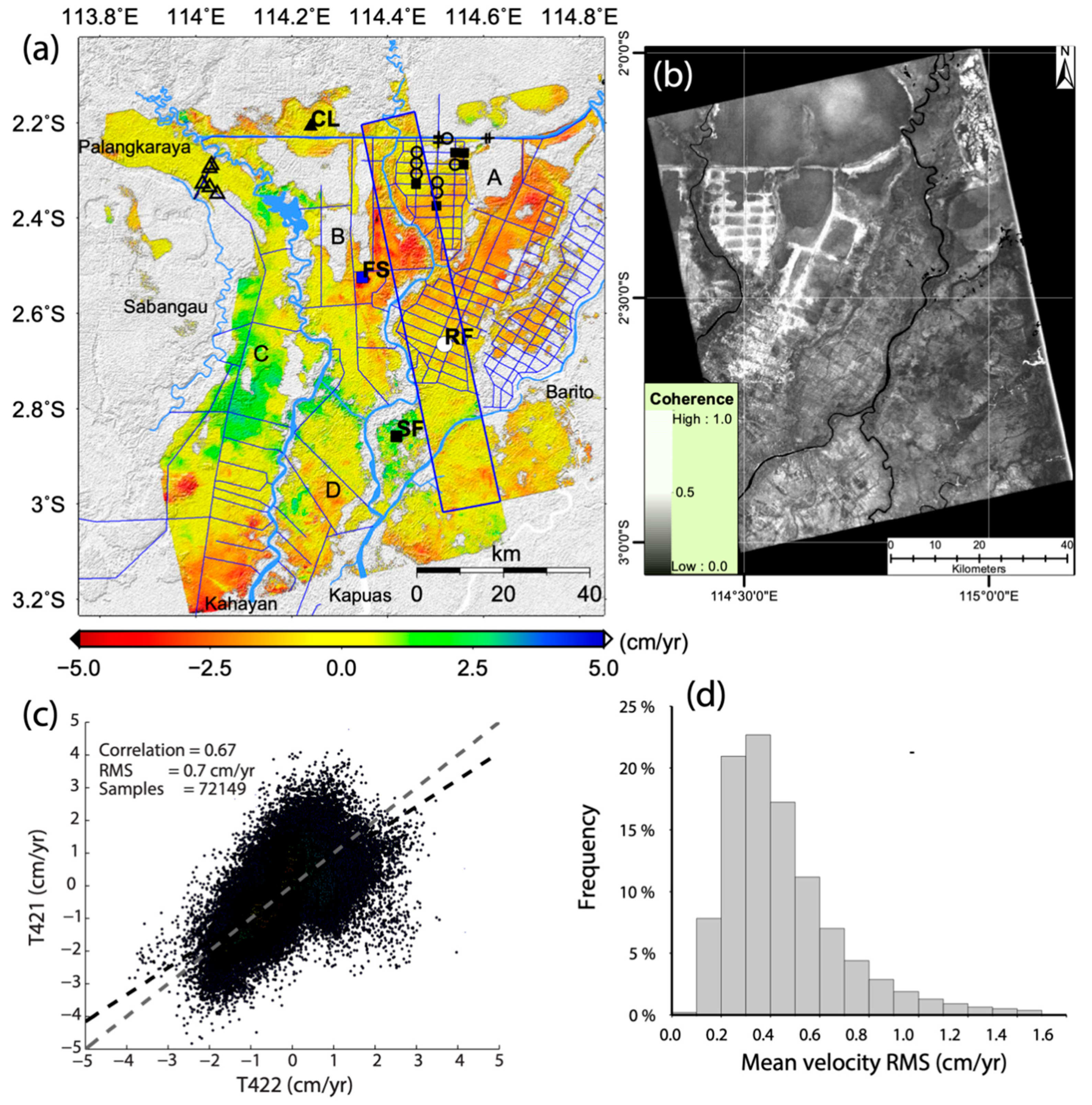
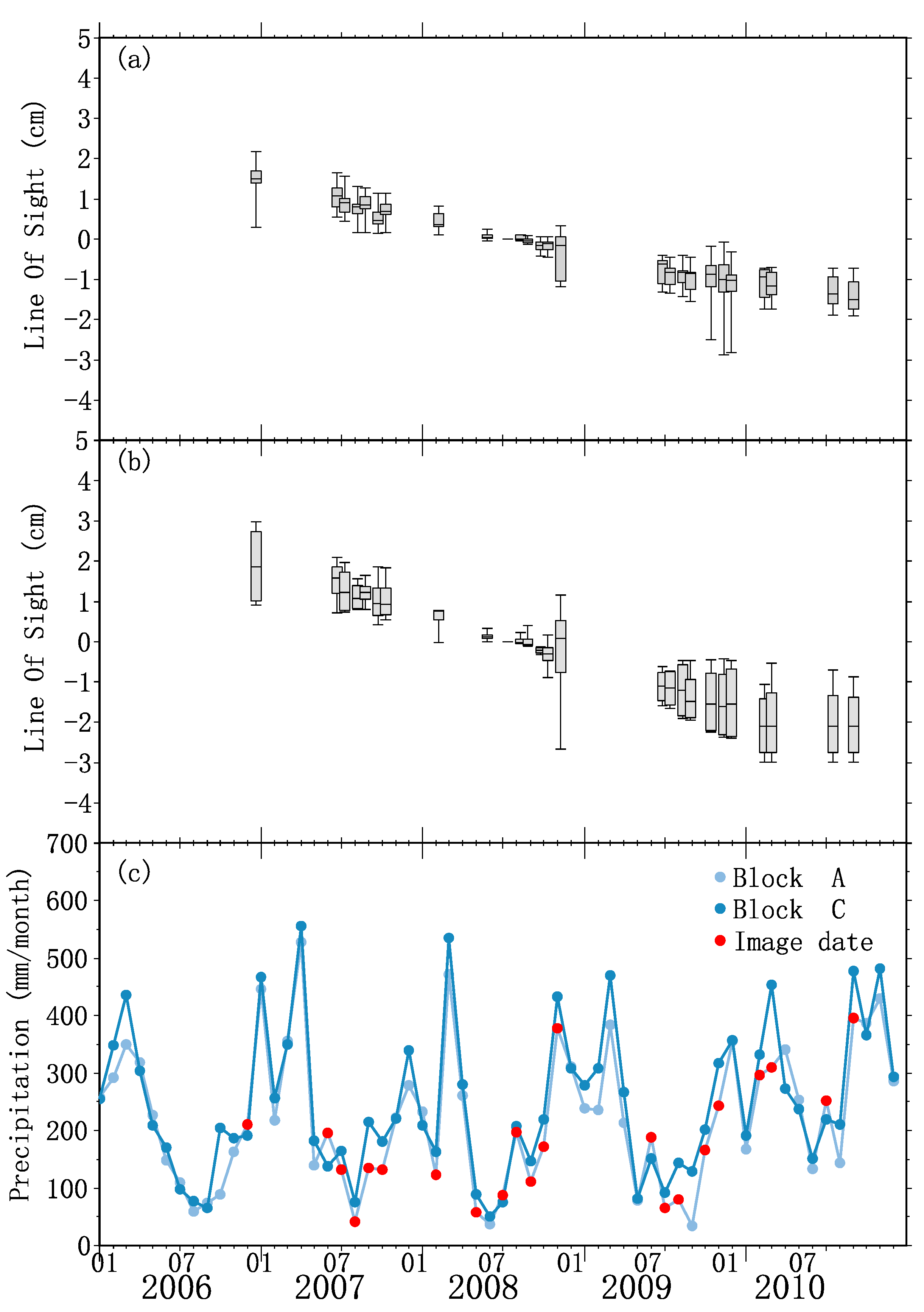
3.1. Mean Height Change Results of the Whole Study Area

Figure 3a shows the final mean height change rate (mean velocity) map along line of sight. Note that the negative value means the surface is moving away from the satellite (‘subsidence’), while the positive value means the surface is moving towards the satellite (‘uplift’). The total number of partially coherent pixels is 859,118 (1,374,913 in total), covering ~62% of the study area, and approximately 73 points/km2 at the case of 90 m resolution. With extensive channels areas in all blocks, subsidence signals can be observed clearly, the largest subsidence rate is more than 5 cm /yr. While the central part of Block C shows uplift signals. Between 2006 and 2010, the mean velocities for Block A, B, C and D are −1.1 ± 1.0 cm/yr, −0.8 ± 1.2 cm/yr, 0.03 ± 1.4 cm/yr and −0.3 ± 1.2 cm/yr respectively. In terms of area, 49% of the study area showed loss in surface height (less than −0.7 cm/yr), 15% retained similar surface height (between −0.7 cm/yr and 0.7 cm/yr), and 37% increased in surface height (greater than 0.7 cm/yr). Figure 3d shows the final root mean square (RMS) of the mean velocity with an average RMS of 0.45 cm/yr.
The spatial pattern of the surface height changes appears to be associated with land use. No obvious surface height change can be observed in Palangkaraya city (NW corner of the study area) during the observation period, which is as would be expected. The drained shrub swamp area in Block B has the largest rate of decrease in surface heights. Much of this rice field areas in Blocks A, C and D show decrease patterns in surface heights. The cleared area has relatively small decreases in surface heights ranging from 0 to 2 cm/yr. In the center of Block C, signals in the secondary swamp forest area show increased surface heights during the observation period, with rates of up to ~3 cm/yr.

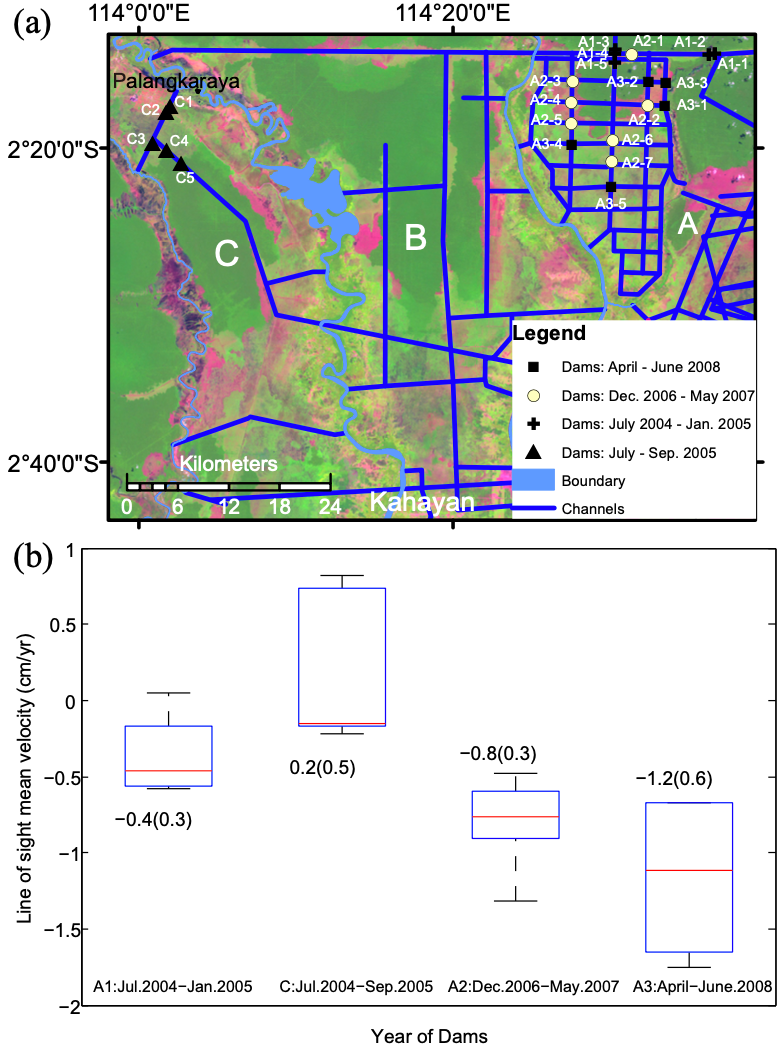
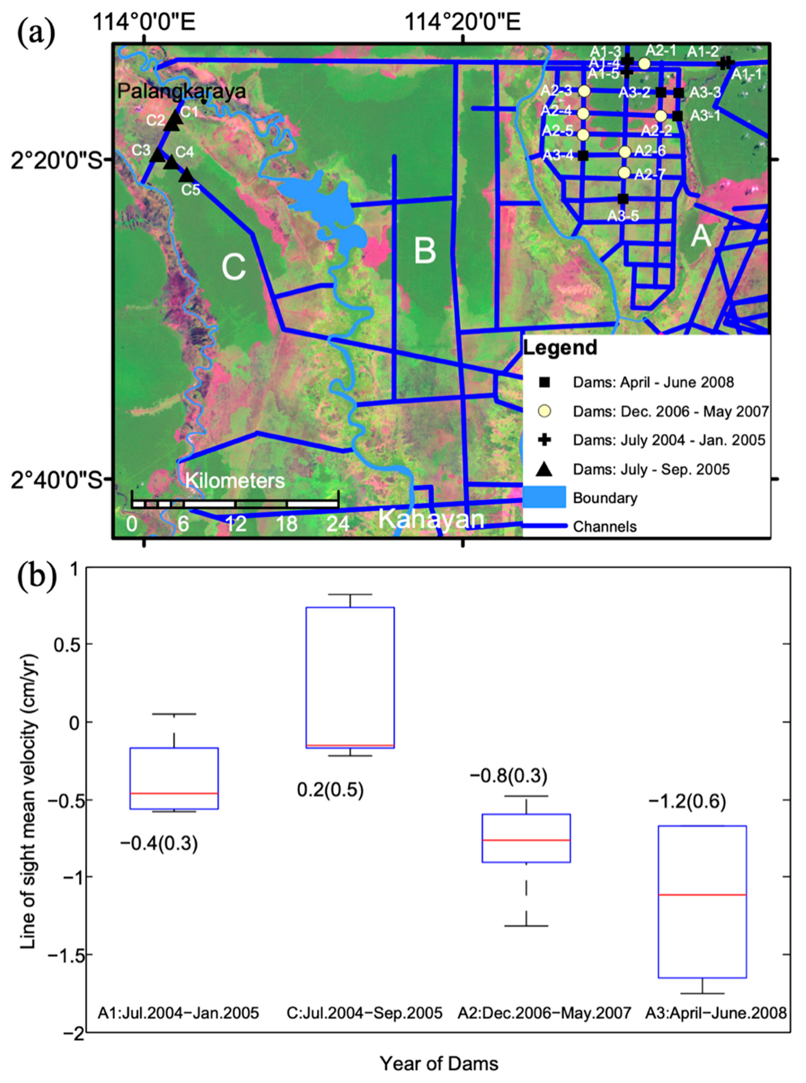
3.2. Peatland Height Changes in Area with Restoration

The locations of the dams and their corresponding mean velocities are shown in Figure 4a,b respectively. Because of the loss of coherence, Points A1-3 and A3-2 are not included in the change rate analysis. In Block A, dams are constructed in different year, completed in January 2005, May 2007 and June 2008 respectively, and their corresponding mean velocities are shown in Table 3. The mean velocities in Block C are shown in Table 3. Note that the closer the mean velocity is to zero, it suggests the bigger impact of the dam construction on reducing the rate of surface height loss along the dams.

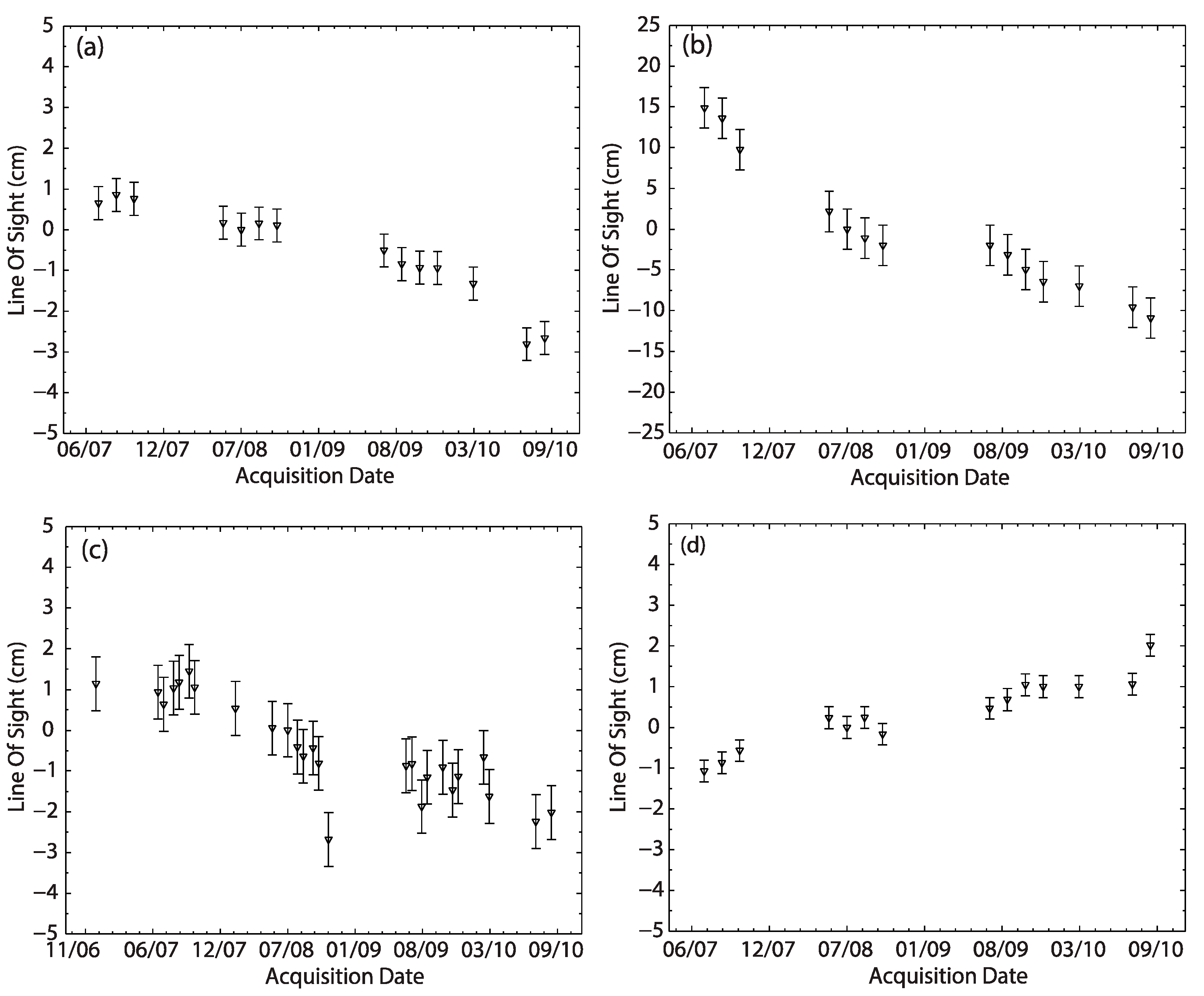
3.3. Peatland Height Changes in Area without Restoration

Figure 5 shows the evolution of peatland height at four points between 2006 and 2010. These four points are distributed in different land uses and have not undergone restoration. In Figure 5a, Point CL located in the cleared area shows peat height to be decreasing at a mean rate of −0.8 cm/yr. Point FS, located within a shrub swamp area (Figure 5b), had the greatest rate of decrease in surface height, by 17 cm during the dry seasons of 2007 to 2008, and 8 cm during 2008 to 2010, a total of 25 cm from 9 July 2007 to 1 September 2010. By checking Landsat images, fire scars can be found from the dry season of 2007 in this area, which may explain why surface lowering was greater between the dry seasons of 2007 to 2008 than during the following two years. Points in the rice field (RF) area exhibited relatively contestant rates of surface height decrease approximately −1.0 cm/yr (Figure 5c). Point SF in the swamp forest shows an increase in surface height with a rate of 1.4 cm/yr. The signals of increasing surface height could be due to the accumulation of peat and /or water-logging changing peat structure (Figure 5d), as this area is not drained by extensive channels.

4. Discussions

Although L-band data is used in this study, coherence is still lost in Block C. As show in Figure 3a, the InSAR results have good spatial coverage across the study area, covering various landscapes (Figure 1). By comparing the final valid pixel distribution in Figure 3a, the average coherence map of Track 421 in Figure 3b and land use map in Figure 1 visually, we observe that loss of coherent pixels is often associated with primary or secondary swamp forest, such as at the western part of Block C, the northern part of Block B, and a small area in the northern part of Block A. The loss of coherence is likely because the density of primary/second swamp forest is higher than 100 t/ha [50], where the radar signals are not able to penetrate it canopy of the forest, it returned radar signals are most likely from the canopy of the forest [51,52]. Therefore, temporal decorrelation occurs even over short time periods. While for forest density below 100 t/ha, L-band radar signals can penetrate canopy and are predominantly reflected from the ground with strong double-bouncing contributions from the trunks [53]. Therefore, stable signals are expected from forest density below 100 t/ha in our final results, such as signals from secondary swamp forest in the center of Block C. The eastern part of Block A also shows loss of coherent pixels, but this is because these areas are relatively-low and close to the river, still resulting in frequent summer flooding in this eastern part of Block A even in summer seasons [36].
L-band data would provide much better coverage than that of C-band. Using C-band data and intermittent coherent pixel algorithm in tropical peatlands, Marshall et al., [24] obtained data coverage over 94.35% of the study area by using a coherence threshold of 0.25 and a recurrence of ~28% in all interferograms. However, the study also claims that if a coherent pixel is recurrent in each interferogram, only 25.35% of the study area would be covered by coherent pixels. In this study, a coherence threshold of 0.3 and a recurrence of 50% in all interferograms strategy is applied, the final partially coherent pixels covers 62% of the study area. In addition, using C-band data and PS-InSAR method, only 333 stable PS points are found in 6 km2 boreal peatlands (~56 PS points /km2), where vegetation is dominated by moss [32].Therefore less stable PS points per km2 are excepted for C-band in tropical peatlands.
The accuracy of the InSAR time series measurements in tropical peatlands is applicable to measure the peatland surface change. Without detailed ground data of this area, cross-validation is achieved by using the overlapping area data from the two independent adjacent tracks. A correlation coefficient of 0.67 was obtained with an RMS of the mean velocity is 0.49 cm/yr implies the InSAR measurement has potential in measuring the tropical peatland height change. The InSAR time series methodology used in this study is also validated by using ground data in other studies, which provide an accuracy of 1.57 cm/yr with a correlation efficient of 0.93 [54]. The accuracy obtained in these studies is also higher than that of ground measurements (e.g., perforated PVC tube inserted vertically in peatlands) [55]. Therefore, InSAR time series and L-band data could be a valuable tool in mapping magnitude and spatial pattern of peatland surface change.
Restoration requires time to take effect [14,15], implying that the earlier the dam is constructed, the more effective its presence will be. This is evidenced by the dams in Blocks A and C (Figure 4b). In Block A, dams completed in January 2005 appears to have more significant restoration effects compared to dams completed in May 2007 and June 2008 (both p < 0.05, Table 4). Similar effects of successful rewetting were considered observed by investigating the backscatter changes of three PALSAR images acquired in August 2007, August 2008 and August 2009 respectively [15].
Our SAR images were acquired from December 2006 to September 2010, nearly two years after the dam construction in Block C. The mean velocities of C1, C2 and C5 are close to zero, which means the areas near the dams are no longer losing height and thus loss of peat is slower. Increases in surface heights are observed in Points C3 and C4. The most plausible reason is that the ground water level increased in dry seasons and the peatland was rewetted, reducing loss of carbon through oxidation and, or, causing the peatland surface to rise or grow. Since the ALOS-1 PALSAR SAR images are only available after December 2006, we obtain the peat height change rates before the completion of the dam construction from a previous study [15]. By analyzing the backscatter changes of Envisat ASAR images acquired between 2004 and 2009, it was observed that backscatter increased in Block C after the completion of the dam construction in September 2005, implying that the peat soil moisture continuously increased with ground water level, even during the very prolonged dry season of 2006 [15]. Before the completion of the dam construction, a small decrease of the backscatter was observed between July 2004 and September 2005, implying that the peatland was continuously drained with a loss of carbon through oxidation, and resulted in losing peat height.
The swelling and shrinking of peat surface caused by changes in water availability (such as precipitation) had limited effects on the subsidence trend. In Block A (Figure 4b), dams were constructed during different periods, with the earliest being constructed in January 2005. The mean velocity of the dams constructed in January 2005 is smaller than the mean velocity of the dams constructed in May 2007, and the mean velocity of the dams constructed in May 2007 is smaller than the mean velocity of the dams constructed in June 2008. Figure 6a,b show LOS surface displacement time series for the A2 and A3 dams, and Figure 6c shows the monthly precipitation data derived from Tropical Rainfall measurement mission product (TRMM_3B43 V7) with a horizontal resolution of 0.25 degrees × 0.25 degrees [56]. For all the dams completed in May 2007, the typical cumulative subsidence is approximately 4 cm between December 2006 and September 2010, and a clear subsidence trend can be observed in Figure 6a. For dams completed in June 2008, a similar subsidence trend can be observed between December 2006 and February 2010. The TRMM precipitation records show seasonal variations (Figure 6c), which cannot be observed in either of the LOS surface displacement time series. This suggests that (i) the swelling and shrinking of peat surface caused by changes in water availability (from precipitation) had limited effects on the subsidence trend, and (ii) the dams completed in May 2007 or in June 2008 had little effects on restoration during our SAR observation period, and a longer time is required to have effects on restoration.
Compared to surface height mapping with GPS or other methods, InSAR provides greater spatial extent in monitoring surface height changes, whilst keeping good precision. However, the InSAR TS + AEM algorithm has its disadvantages. For tropical peatland areas, there is often lack in sufficient number of L-band images within the same path and frame required for InSAR measurement. The lack of sufficient number of SAR images may make it difficult to detect adequate coherent pixels, and separate displacement signals from noises (e.g., the APS noise). For example, there are less than 20 L-band radar images acquired in this study area within the same path and frame by the current ALOS-2 satellite from 2014 to now. By comparison, there are more than 100 Sentinel-1A/B C-band radar images within the same path and frame over the same period. In addition, the use of L-band images could not detect low rate of motion in peatlands, as longer wavelengths tend to be less sensitive to small changes.

5. Conclusions

Here we show that InSAR time series analysis of L-band data may be of considerable value in monitoring restoration effects in peatlands. Our analysis suggests that the restoration does have an impact and its effectiveness increases with construction time—the earlier the dam is constructed, the more significant the restoration is. The InSAR time series also provides insight in the likely relative magnitude and spatial pattern of damage to peatland caused by drainage and fires. To confirm the value of using InSAR time series, targeted fieldwork would help corroborate the InSAR understanding and also offer insight into why there are periods and areas of loss of coherence. With such security of understanding the community could proceed to using InSAR time series to make temporal and regional assessment of a landscape response to anthropogenic activity and guide future restoration activities. With this capacity InSAR offers a great advantage over field-based point observations by offering regional coverage, and provides a practical way to monitor peatland height changes continuously and globally, with the archived JERS/ALOS-1 dataset and the operational ALOS-2.

Author Contributions

Conceptualization, Z.Z., Z.L., and S.W.; data curation, Z.Z.; formal analysis, Z.Z.; funding acquisition, Z.L. and S.W.; investigation, Z.Z., Z.L., and S.W.; methodology, Z.Z. and Z.L.; project administration, Z.L. and S.W.; resources, Z.L., S.W., and A.T.; supervision, Z.L. and S.W.; validation, Z.Z.; visualization, Z.Z.; writing—original draft, Z.Z.; writing—review and editing, Z.L. and S.W.

Funding

Zhou was supported by the National Natural Science Foundation of China (Grant No. 41804017), by the Strategic Priority Research Program of the Chinese Academy of Sciences (Grant No. XDA19070104), by a China Scholarship Council (CSC) scholarship and the University of Glasgow. The work was supported the UK Natural Environment Research Council (NERC) through the Centre for the Observation and Modelling of Earthquakes, Volcanoes and Tectonics (COMET) and the GAS and LICS projects (Ref: NE/H001085/1 and NE/K010794/1 respectively) as well as the ESA-MOST DRAGON-3 projects (Ref: 10607 and 10665). METI (Japanese Ministry of Economy, Trade and Industry) and JAXA (Japan Aerospace Exploration Agency) retain ownership of the original ALOS PALSAR data used for this study, which were distributed by the Earth Remote Sensing Data Analysis Center.

Acknowledgments

Thanks to Stefano Tebaldini for reviewing this paper before submission.

Conflicts of Interest

The authors declare no conflict of interest.

References

  1. Yu, Z.; Loisel, J.; Brosseau, D.P.; Beilman, D.W.; Hunt, S.J. Global peatland dynamics since the last glacial maximum. Geophys. Res. Lett. 2010, 37, L13402. [Google Scholar] [CrossRef]
  2. Grace, J. Understanding and managing the global carbon cycle. J. Ecol. 2004, 92, 189–202. [Google Scholar] [CrossRef]
  3. Page, S.E.; Baird, A.J. Peatlands and global change: Response and resilience. Annu. Rev. Environ. Resour. 2016, 41, 35–57. [Google Scholar] [CrossRef]
  4. Jukka, M.; Aljosja, H.; Ronald, V.; Soo Chin, L.; Susan, E.P. From carbon sink to carbon source: Extensive peat oxidation in insular southeast asia since 1990. Environ. Res. Lett. 2017, 12, 024014. [Google Scholar]
  5. Page, S.E.; Rieley, J.O.; Banks, C.J. Global and regional importance of the tropical peatland carbon pool. Glob. Chang. Biol. 2011, 17, 798–818. [Google Scholar] [CrossRef] [Green Version]
  6. Dohong, A.; Aziz, A.A.; Dargusch, P. A review of the drivers of tropical peatland degradation in south-east asia. Land Use Policy 2017, 69, 349–360. [Google Scholar] [CrossRef]
  7. Austin, K.G.; Schwantes, A.; Gu, Y.; Kasibhatla, P.S. What causes deforestation in indonesia? Environ. Res. Lett. 2019, 14, 024007. [Google Scholar] [CrossRef]
  8. Stibig, H.J.; Achard, F.; Carboni, S.; Raši, R.; Miettinen, J. Change in tropical forest cover of southeast asia from 1990 to 2010. Biogeosciences 2014, 11, 247–258. [Google Scholar] [CrossRef]
  9. Lawrence, D.; Vandecar, K. Effects of tropical deforestation on climate and agriculture. Nat. Clim. Chang. 2014, 5, 27. [Google Scholar] [CrossRef]
  10. Wösten, J.H.M.; Ismail, A.B.; van Wijk, A.L.M. Peat subsidence and its practical implications: A case study in malaysia. Geoderma 1997, 78, 25–36. [Google Scholar] [CrossRef]
  11. Couwenberg, J.; Dommain, R.; Joosten, H. Greenhouse gas fluxes from tropical peatlands in south-east asia. Glob. Chang. Biol. 2010, 16, 1715–1732. [Google Scholar] [CrossRef]
  12. Page, S.; Siegert, F.; Rieley, J.O.; Boehm, H.-D.V.; Jaya, A.; Limin, S. The amount of carbon released from peat and forest fires in indonesia during 1997. Nature 2002, 420, 61–65. [Google Scholar] [CrossRef] [PubMed]
  13. Sasha, A.; Cara, R.N.; James, A.; David, L.; An, C.; Kevin, L.E.; Finlayson, C.M.; Rudolf, S.d.G.; Jim, A.H.; Eric, S.H.; et al. Opportunities and challenges for ecological restoration within redd+. Restor. Ecol. 2011, 19, 683–689. [Google Scholar]
  14. Wösten, J.H.M.; Clymans, E.; Page, S.E.; Rieley, J.O.; Limin, S.H. Peat–water interrelationships in a tropical peatland ecosystem in southeast asia. CATENA 2008, 73, 212–224. [Google Scholar] [CrossRef]
  15. Jaenicke, J.; Englhart, S.; Siegert, F. Monitoring the effect of restoration measures in indonesian peatlands by radar satellite imagery. J. Environ. Manag. 2011, 92, 630–638. [Google Scholar] [CrossRef] [PubMed]
  16. CKPP. Provisional Report of theCentral Kalimantan Peatland Project; CKPP Consortium: Palangka Raya, Indonesia, 2008; p. 70. [Google Scholar]
  17. Hanssen, R.F. Radar Interferometry:Data Interpretation and Error Analysis; Kluwer Academic Plublishers: Dordrecht, The Netherland, 2001. [Google Scholar]
  18. Osmanoğlu, B.; Sunar, F.; Wdowinski, S.; Cabral-Cano, E. Time series analysis of insar data: Methods and trends. Isprs J. Photogramm. Remote Sens. 2016, 115, 90–102. [Google Scholar] [CrossRef]
  19. Massonnet, D.; Feigl, K.L. Radar interferometry and its application to changes in the earth’s surface. Rev. Geophys. 1998, 36, 441–500. [Google Scholar] [CrossRef]
  20. Cigna, F.; Sowter, A.; Jordan, C.J.; Rawlins, B.G. ntermittent small baseline subset (ISBAS) monitoring of land covers unfavourable for conventional C-band InSAR: Proof-of-concept for peatland environments in North Wales, UK. In Proceedings of the SPIE—The International Society for Optical Engineering, Amsterdam, The Netherlands, 22 September 2014; pp. 924305–924306. [Google Scholar]
  21. Dahdal, B. The Use of Interferometric Spaceborne Radar and GIS to Measure Peat Subsidence in Indonesia. Ph.D. Thesis, University of Leicester, Leicester, UK, 2011. [Google Scholar]
  22. Zhou, Z.; Waldron, S.; Li, Z. Quantifying Changes in Land-Surface Height in Bioenergy Palm Oil Plantations (Sumatra) Using Insar Time Series; EGU: Vienna, Austria, 2013; Volume 15, p. 13128. [Google Scholar]
  23. Zhou, Z. The Applications of Insar Time Series Analysis for Monitoring Long-Term Surface Change in Peatlands. Ph.D. Thesis, University of Glasgow, Glasgow, UK, 2013. [Google Scholar]
  24. Marshall, C.; Large, D.J.; Athab, A.; Evers, S.L.; Sowter, A.; Marsh, S.; Sjögersten, S. Monitoring tropical peat related settlement using isbas insar, kuala lumpur international airport (klia). Eng. Geol. 2018, 244, 57–65. [Google Scholar] [CrossRef]
  25. Alshammari, L.; Large, J.D.; Boyd, S.D.; Sowter, A.; Anderson, R.; Andersen, R.; Marsh, S. Long-term peatland condition assessment via surface motion monitoring using the isbas dinsar technique over the flow country, scotland. Remote Sens. 2018, 10, 1102–1125. [Google Scholar] [CrossRef]
  26. Chaussard, E.; Hoyt, A.; Harvey, C. Bridging earth systems sciences with insar: From quantifying land subsidence to estimating the CO2 emissions associated with peatlands oxidation following deforestation in southeast asia. In AGU Fall Meeting Abstracts; AGU: Washington, DC, USA, 2018; p. G53B-07. [Google Scholar]
  27. Susanti, R.D.; Anjasmara, I.M. Analysing peatland subsidence in pelalawan regency, riau using dinsar method. Iptek J. Proc. Ser. 2019, 2, 60–64. [Google Scholar] [CrossRef]
  28. Meng, W.; Sandwell, D.T. Decorrelation of l-band and c-band interferometry over vegetated areas in california. Geosci. Remote Sens. IEEE Trans. 2010, 48, 2942–2952. [Google Scholar] [CrossRef]
  29. Ferretti, A.; Prati, C.; Rocca, F. Permanent scatterers in sar interferometry. Geosci. Remote Sens. IEEE Trans. 2001, 39, 8–20. [Google Scholar] [CrossRef]
  30. Berardino, P.; Fornaro, G.; Lanari, R.; Sansosti, E. A new algorithm for surface deformation monitoring based on small baseline differential sar interferograms. Geosci. Remote Sens. IEEE Trans. 2002, 40, 2375–2383. [Google Scholar] [CrossRef]
  31. Ferretti, A.; Fumagalli, A.; Novali, F.; Prati, C.; Rocca, F.; Rucci, A. A new algorithm for processing interferometric data-stacks: Squeesar. Geosci. Remote Sens. IEEE Trans. 2011, 49, 1–11. [Google Scholar] [CrossRef]
  32. Fiaschi, S.; Holohan, P.E.; Sheehy, M.; Floris, M. Ps-insar analysis of sentinel-1 data for detecting ground motion in temperate oceanic climate zones: A case study in the republic of ireland. Remote Sens. 2019, 11, 347–376. [Google Scholar] [CrossRef]
  33. Jaenicke, J.; Wösten, H.; Budiman, A.; Siegert, F. Planning hydrological restoration of peatlands in indonesia to mitigate carbon dioxide emissions. Mitig Adapt. Strat. Glob. Chang. 2010, 15, 223–239. [Google Scholar] [CrossRef]
  34. Kementerian Kehutanan Republik Indonesia. WebGIS Kehutanan. Available online: http://appgis.dephut.go.id/appgis/kml.aspx (accessed on 3 February 2012).
  35. Page, S.; Hosciło, A.; Wösten, H.; Jauhiainen, J.; Silvius, M.; Rieley, J.; Ritzema, H.; Tansey, K.; Graham, L.; Vasander, H.; et al. Restoration ecology of lowland tropical peatlands in southeast asia: Current knowledge and future research directions. Ecosystems 2009, 12, 888–905. [Google Scholar] [CrossRef]
  36. Hoekman, D.H. Monitoring Tropical Peat Swamp Deforestation and Hydrological Dynamics by ASAR and PALSAR; InTech: London, UK, 2009; pp. 257–275. [Google Scholar]
  37. Hoekman, D.H. Satellite radar observation of tropical peat swamp forest as a tool for hydrological modelling and environmental protection. Aquat. Conserv. Mar. Freshw. Ecosyst. 2007, 17, 265–275. [Google Scholar] [CrossRef]
  38. Rosen, P.A.; Hensley, S.; Peltzer, G.; Simons, M. Updated repeat orbit interferometry package released. Eos. Trans. Agu. 2004, 85, 47. [Google Scholar] [CrossRef]
  39. Farr, T.G.; Rosen, P.A.; Caro, E.; Crippen, R.; Duren, R.; Hensley, S.; Kobrick, M.; Paller, M.; Rodriguez, E.; Roth, L.; et al. The shuttle radar topography mission. Rev. Geophys. 2007, 45, RG2004. [Google Scholar] [CrossRef]
  40. Chen, C.W.; Zebker, H.A. Phase unwrapping for large sar interferograms: Statistical segmentation and generalized network models. Geosci. Remote Sens. IEEE Trans. 2002, 40, 1709–1719. [Google Scholar] [CrossRef]
  41. Biggs, J.; Wright, T.; Lu, Z.; Parsons, B. Multi-interferogram method for measuring interseismic deformation: Denali fault, alaska. Geophys. J. Int. 2007, 170, 1165–1179. [Google Scholar] [CrossRef]
  42. Hooper, A.; Segall, P.; Zebker, H. Persistent scatterer interferometric synthetic aperture radar for crustal deformation analysis, with application to volcán alcedo, galápagos. J. Geophys. Res. 2007, 112, B07407. [Google Scholar] [CrossRef]
  43. Doin, M.-P.; Guillaso, S.; Jolivet, R.; Lasserre, C.; Lodge, F.; Ducret, G.; Grandin, R. Presentation of the Small-Baseline NSBAS Processing Chain on a Case Example: The ETNA Deformation Monitoring from 2003 to 2010 Using Envisat Data; ESA: Paris, France, 2011; pp. 303–304. [Google Scholar]
  44. Li, Z.; Fielding, E.J.; Cross, P. Integration of insar time-series analysis and water-vapor correction for mapping postseismic motion after the 2003 bam (iran) earthquake. Geosci. Remote Sens. IEEE Trans. 2009, 47, 3220–3230. [Google Scholar]
  45. Zhang, L.; Ding, X.; Lu, Z. Ground settlement monitoring based on temporarily coherent points between two sar acquisitions. Isprs J. Photogramm. Remote Sens. 2011, 66, 146–152. [Google Scholar] [CrossRef]
  46. Sowter, A.; Bateson, L.; Strange, P.; Ambrose, K.; Syafiudin, M.F. Dinsar estimation of land motion using intermittent coherence with application to the south derbyshire and leicestershire coalfields. Remote Sens. Lett. 2013, 4, 979–987. [Google Scholar] [CrossRef]
  47. Li, Z.; Fielding, E.J.; Cross, P.; Muller, J.-P. Interferometric synthetic aperture radar atmospheric correction: Gps topography-dependent turbulence model. J. Geophys. Res. Solid Earth 2006, 111, B02404. [Google Scholar] [CrossRef]
  48. Williams, S.; Bock, Y.; Fang, P. Integrated satellite interferometry: Tropospheric noise, gps estimates and implications for interferometric synthetic aperture radar products. J. Geophys. Res. Solid Earth 1998, 103, 27051–27067. [Google Scholar] [CrossRef]
  49. Hammond, W.C.; Blewitt, G.; Li, Z.; Plag, H.P.; Kreemer, C. Contemporary uplift of the sierra nevada, western united states, from gps and insar measurements. Geology 2012, 40, 667–670. [Google Scholar] [CrossRef]
  50. Treuhaft, R.N.; Gonçalves, F.G.; Drake, J.B.; Chapman, B.D.; dos Santos, J.R.; Dutra, L.V.; Graça, P.M.L.A.; Purcell, G.H. Biomass estimation in a tropical wet forest using fourier transforms of profiles from lidar or interferometric sar. Geophys. Res. Lett. 2010, 37, L23403. [Google Scholar] [CrossRef]
  51. Imhoff, M.L. Radar backscatter/biomass saturation: Observations and implications for global biomass assessment. In Proceedings of the IGARSS’93—IEEE International Geoscience and Remote Sensing Symposium, Tokyo, Japan, 18–21 August 1993; pp. 43–45. [Google Scholar]
  52. Luckman, A.; Baker, J.; Honzák, M.; Lucas, R. Tropical forest biomass density estimation using jers-1 sar: Seasonal variation, confidence limits, and application to image mosaics. Remote Sens. Environ. 1998, 63, 126–139. [Google Scholar] [CrossRef]
  53. Bamler, R.; Hartl, P. Synthetic aperture radar interferometry. Inverse Probl. 1998, 14, 1–54. [Google Scholar] [CrossRef]
  54. Zhou, W.; Li, S.; Zhou, Z.; Chang, X. Remote sensing of deformation of a high concrete-faced rockfill dam using insar: A study of the shuibuya dam, china. Remote Sens. 2016, 8, 255–269. [Google Scholar] [CrossRef]
  55. Hooijer, A.; Page, S.; Jauhiainen, J.; Lee, W.A.; Lu, X.X.; Idris, A.; Anshari, G. Subsidence and carbon loss in drained tropical peatlands. Biogeosciences 2012, 9, 1053–1071. [Google Scholar] [CrossRef] [Green Version]
  56. TRMM. InTropical Rainfall Measuring Mission. Available online: http://disc.gsfc.nasa.gov/datacollection/TRMM_3B43_V7.shtml (accessed on 5 June 2015).
Figure 1. The location of this study area and distribution of land uses. Pink boxes denote the coverage of ALOS PALSAR images (Tracks 422 and 421). The four blocks of area (A–D) are indicated by light blue outlines. Land use information in this diagram is taken from Kementerian Kehutanan Republik Indonesia [34]. The red square in the top right corner is the location of this study area.
Remotesensing 11 02592 g001
Figure 2. Small baseline interferograms generated from ALOS PALSAR Tracks 421 (a) and 422 (b) respectively. Each black triangle denotes one SAR image, and black solid lines between two black triangles represent interferograms. The red square marks the reference date for time series analysis.
Remotesensing 11 02592 g002
Figure 3. Mean height change rate map and correlation analyses: (a) mean velocity map between 2006 and 2010, light blue curves represent block boundaries and solid blue lines represent channels; negative value means subsidence and positive value means increase in height; dots CL, FS, RF and SF are four time series analysis sites, other triangles and square dots in Block A and C are dams; (b) The average coherence of 27 interferograms from Track T421, a pixel with coherence great than 0.3 presents a stable signal; (c) correlation of the mean velocities over the overlapping area between the two adjacent tracks 422 and 421 (Figure 1): the gray dash line indicates the 1:1 line and the black dash line indicates the best fitted line; and (d) the RMS histogram of the mean velocity map.
Remotesensing 11 02592 g003
Figure 4. The location of Dams (a) and their corresponding mean velocity statistics analysis (b) in Blocks A and C. In (b), for each box, the central red line is the median, the edges of the box are the 25th and 75th percentiles, and whiskers represent the minimum and maximum values. Different construction dates of dams are denoted by different codes. Successful damming is considered to raise the ground water level and decrease the velocity of loss of surface heights. Each value corresponds to the mean velocity of 9 points within a 270 m by 270 m window.
Remotesensing 11 02592 g004
Figure 5. Time series of four points (CL, FS, RF and SF) located in areas with different land uses: (a) for CL point in cleared area, (b) for FS point in fire scar area, (c) for RF point in rice field area and (d) for SF point in secondary swamp forest area. Each point presents one SAR image acquisition date. Each value corresponds to the mean of points within a 270 m by 270 m window and the error bars represent the associated standard deviation. Note the scales in the Y-axis are not identical; the zero value corresponds to the reference image, which is acquired on 9th September 2008.
Remotesensing 11 02592 g005
Figure 6. LOS surface displacement time series for (a) 7 dams constructed during the period from December 2006 to May 2007, (b) 4 dams constructed during the period from April to June 2008, and (c) the corresponding TRMM precipitation records (red dots). In Figure 6a,b, for each box, the central line is the median, the edges of the box are the 25th and 75th percentiles, and whiskers represent the minimum and maximum values. In Figure 6c, the blue dots present the TRMM record for Block C, while the light blue dots present for Black A. Note: (1) LOS surface displacements correspond to the mean LOS surface displacement of all the points within a 270 m by 270 m window, and (2) the reference date is 9 September 2008.
Remotesensing 11 02592 g006
Table 1. ALOS images from Tracks 421 and 422 used in this study. Dates are given in Year-Month-Day (YYYYMMDD) format, and as number of days since the first image for each track. Perpendicular baselines (satellite separation) for Tracks 421 and 422 are relative to the reference dates that were chosen because of limited atmospheric effects on these two SAR images, assessed by checking all interferograms involved SAR images acquired on these dates.
T421T422
Image NumberDateTemporal Baseline (Days)Perpendicular Baseline (m)Image NumberDateTemporal Baseline (Days)Perpendicular Baseline (m)
1200612200139.61200707090228.3
220070622184101.122007082446307.4
320070807230208.532007100992129.4
420070922276−245.5420080526322−331.6
520080207414−16.15200807113680.0
6200808095980.0620080826414−255.8
720080924644494.1720081011460471.2
820081109690444.7820090714736638.1
920090627920332.8920090829782741.1
1020090812966−27.91020091014828396.0
1120091112105887.51120091129874266.3
12201002121150234.91220100301966136.9
13201007171104−45.7
1420100901115059.8
Table 2. Location and land use type of points selected in this study.
PointsLongitude (Degrees)Latitude (Degrees)Land Use Type
CL114.2395−2.2077Cleared
FS114.3467−2.5248Fire scar (in shrub swamp)
RF114.51862.6655Rice field
SF114.4182−2.8581Secondary swamp forest
Table 3. Different types of dam and their corresponding mean velocities.
Dam LocationDam Completed
Date
Minimum Mean
Velocities (cm/yr)
Max Mean
Velocities (cm/yr)
Mean (cm/yr)Std (cm/yr)
A1January 2005−0.5−0.10.40.3
A2May 2007−1.4−0.50.80.3
A3June 2008−1.7−0.6−1.20.6
CSeptember 2005−0.250.750.20.5
Table 4. Unpaired T-test for the mean velocities of the dams in Block A. Dams A1, A2, and A3 were completed in January 2005, May 2007, and June 2008, respectively.
p ValueA1A2A3
A1 0.04150.0465
A20.0415 0.1779
A30.04650.1779

