Fuzzy Object-Based Image Analysis Methods Using Sentinel-2A and Landsat-8 Data to Map and Characterize Soil Surface Residue

Abstract

Soil degradation, defined as the lowering and loss of soil functions, is becoming a serious problem worldwide and threatens agricultural production and terrestrial ecosystems. The surface residue of crops is one of the most effective erosion control measures and it increases the soil moisture content. In some areas of the world, the management of soil surface residue (SSR) is crucial for increasing soil fertility, maintaining high soil carbon levels, and reducing the degradation of soil due to rain and wind erosion. Standard methods of measuring the residue cover are time and labor intensive, but remote sensing can support the monitoring of conservation tillage practices applied to large fields. We investigated the potential of per-pixel and object-based image analysis (OBIA) for detecting and estimating the coverage of SSRs after tillage and planting practices for agricultural research fields in Iran using tillage indices for Landsat-8 and novel indices for Sentinel-2A. For validation, SSR was measured in the field through line transects at the beginning of the agricultural season (prior to autumn crop planting). Per-pixel approaches for Landsat-8 satellite images using normalized difference tillage index (NDTI) and simple tillage index (STI) yielded coefficient of determination (R²) values of 0.727 and 0.722, respectively. We developed comparable novel indices for Sentinel-2A satellite data that yielded R² values of 0.760 and 0.759 for NDTI and STI, respectively, which means that the Sentinel data better matched the ground truth data. We tested several OBIA methods and achieved very high overall accuracies of up to 0.948 for Sentinel-2A and 0.891 for Landsat-8 with a membership function method. The OBIA methods clearly outperformed per-pixel approaches in estimating SSR and bear the potential to substitute or complement ground-based techniques.

1. Introduction

The world population is expected to reach 9.1 billion people by 2050. This will require the production of 3 billion tons of cereals annually, up from today’s nearly 2.1 billion tons for both food and animal feed [1]. Therefore, the use of conservation agricultural methods is necessary to protect water and soil, which are the main sources of agricultural productions [2,3].

Conservation tillage systems are an important conservation strategy in agriculture. Residues are left from the previous cultivation on the soil surface in order to protect the soil from water and wind erosion [4]. A residue cover has several important advantages: it increases the soil organic matter [5], speeds up enzymatic activities [6], decreases the soil temperature [7], and reduces the water consumption [8]. In conservation tillage systems, at least 30% of the previous crop residues are left on the soil surface after tillage and planting operations [9]. Depending on the amount of soil surface residue (SSR), conservation tillage systems include minimum (ridge tillage and mulch tillage) and no tillage. In a no-tillage system, the seeding operation is carried out directly into the standing stubble of the previous crops [9].

Various field measurement methods have been developed to estimate the SSR, including line transect, photo comparison, and computational methods. While line transect is a highly accurate field method, it is hardly applicable to large areas due to the time and labor costs. Therefore, several studies aimed to utilize recent developments of remote sensing instruments (satellite, airborne, and unmanned aerial vehicle (UAV)-based sensors) to estimate the SSR [10,11,12,13,14]. To this end, due to the absorption properties of the SSR, the region of 2100 nm of electromagnetic spectrum was studied [15,16]. In this region, the presence of lignin, cellulose, and other saccharides in the external wall of the residue allows distinguishing the SSR signal from soil and vegetation signals [17]. In fact, several methods have been developed for deriving the SSR from spectral images. The majority of approaches calculate the brightness of pixels while object-based image analysis (OBIA) takes other factors, such as texture, color, and geometry of the resulting objects into consideration in addition to brightness.

Several laboratory and field studies have been conducted using per-pixel methods for the identification and mapping of the SSR. van-Deventer et al. [18] developed multispectral Landsat-based indices, including the simple tillage index (STI) and normalized difference tillage index (NDTI), for classifying tillage practices based on the percentage of residue cover. They found that bands of 5 and 7 due to covering the region near 2100 nm are suitable for the estimation of the SSR. Earlier studies applied NDTI and STI indices to multispectral Landsat 6, 7, and 8 images [19,20,21] and obtained accurate results.

Daughtry et al. [22] developed a cellulose absorption index (CAI) from hyper-spectral AVIRIS data as another tillage index and found it to be superior to multispectral Landsat 6 tillage indices. The lignin cellulose index and the shortwave infrared normalized difference residue index were two other multispectral tillage indices based on advanced spaceborne thermal emission and reflection radiometer data, which are superior to the Landsat-based tillage indices, but not as good as the CAI in terms of mapping and characterizing the SSR [23]. Jin et al. [21] increased the accuracy of the detection of SSR by integrating Landsat-8 based tillage indices and gray level co-occurrence matrix (GLCM) textural features.

Pacheco and McNairn [24] obtained coefficient of determination (R²) values of 0.58–0.78 when identifying corn, small grains, and soybean residues from the soil using a pixel-based spectral unmixing analysis method. Sudheer et al. [25] applied an artificial neural network model to detect and map the SSR using Landsat-5 data and obtained overall accuracies of 0.74–0.91 for experimental fields. Bocco et al. [26] estimated corn SSR with an R² value of 0.95 using an artificial neural network model from Landsat-7 data.

In the context of this state of the art in literature, we believe that applying OBIA to SSR is a novelty and we will investigate its potential in the remainder of this article. Over the last years, the number of applications that conceptually aim for objects—still built on the information of the underlying pixels—rose quickly. Blaschke et al. [27] identified a high number of relevant publications that use OBIA concepts and even claim that this concept and its instantiation to a particular order of scale—the geographic, as opposed to applications in medical imaging or cell biology—is a new paradigm in remote sensing. For this level of scale and geodomain, this paradigm is also referred to as geographic object-based image analysis (GEOBIA). In essence, an OBIA process typically groups similar pixels within an image through an image segmentation approach by either merging pixels or by splitting the image iteratively. Both strategies—as well as in other segmentation approaches not discussed herein—will result in relatively homogenous image objects. ‘Relative’ means compared to their surroundings. In the classification step, objects are assigned to a particular class based on a set of classification rules.

There have been very few studies on the application of OBIA for identifying and mapping the SSR. Najafi et al. [28] applied OBIA and Landsat-8 images to classify the SSR into the following three classes: SSR < 30%, SSR 30%–60%, and SSR > 60%.

OBIA is a field within remote sensing and image processing that bridges geographic information science (GIScience, in short). In this article, we highlight two groups of classification approaches based on fuzzy object-based image analysis, namely, a) membership functions and b) nearest neighbor (NN). From its onset, OBIA has often been associated with fuzzy methods, where objects are assigned to a particular class based on fuzzy relations and rules. Many studies illustrate how to assign particular objects to classes based on obtained fuzzy membership values for each object class and fuzzy rules combining several such rules [29,30,31,32,33].

OBIA methods have already been used to identify landslides, debris-covered glaciers, and vegetation [34]. Kalantar et al. [35] applied an OBIA method to identify land cover features using spectral UAV images. They found that OBIA performed well in comparison to decision tree and support vector machine methods. The accuracy of the results of OBIA is strongly influenced by the selection of fuzzy operators and membership functions [36]. The nearest neighbor (NN) classifier algorithm aims to classify images based on similarities of object values in the determined features [37,38]. Yu et al. [39] applied an object-based NN classification for land cover mapping using high-resolution UAV spectral images. They considered 52 object-based features in terms of their spectral properties, texture features, topography, and object geometry in a feature space. Blaschke et al. [37] also investigated the capability of OBIA and NN classification algorithms (spectral, GLCM textural features, and geometry features) for detecting and identifying landslide locations with a semi-automated approach. The capability of the NN method was also reported in other studies [40,41].

Based on the above-mentioned justifications, the objectives of this study are a) to describe a novel method based on fuzzy OBIA for extracting and mapping SSR and tillage intensity, b) to compare the capability of Landsat-8 and Sentinel-2A satellite images for mapping the residue cover, and c) to investigate the accuracy of per-pixel and object-based image analysis approaches and their respective indices and algorithms for residue cover assessment.

2. Materials and Methods

2.1. Study Area

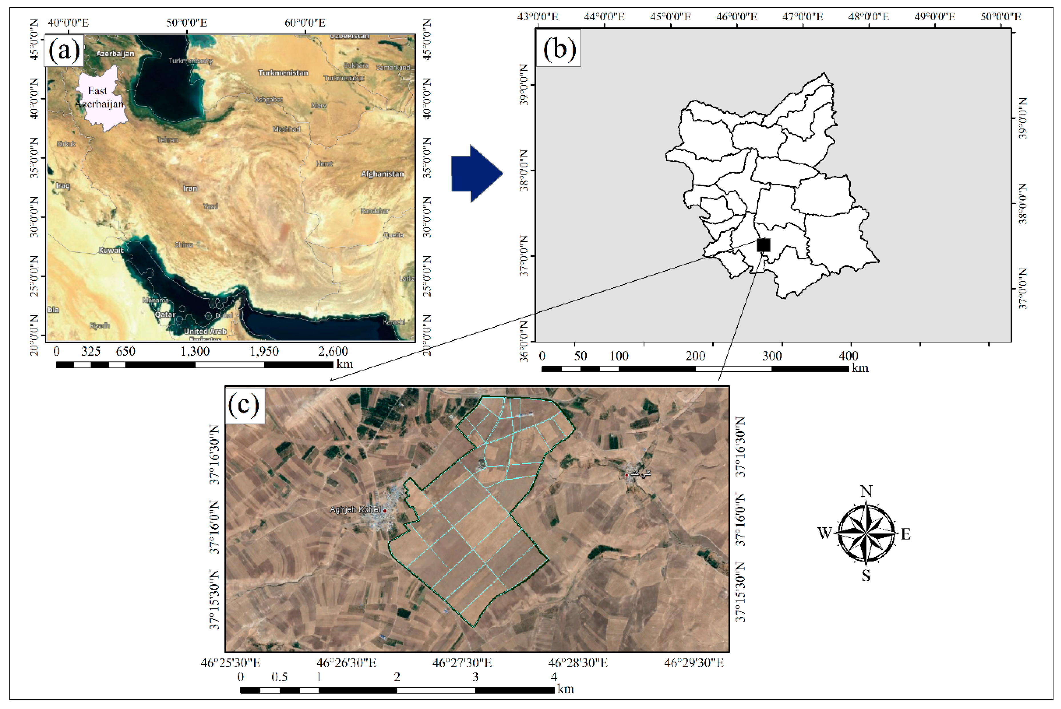
Ground truth data of tillage and planting operations were collected within an agricultural area operated by the Dryland Agricultural Research Institute of Iran’s East Azerbaijan province located at 46° 27′ 29″ E, 37° 15′ 36″ N. The cropping system at the study site was composed of wheat, pea, and forage crops. Different conservation methods and intensive tillage methods were carried out in the study area as tillage/planting practices. As a result, a wide range of SSR levels from full residue cover to bare soil was available across the study area (Figure 1). In this article, we investigate the agricultural system of the study area with respect to environmental issues such as water scarcity and soil erosion. The outcome of this research shall serve as an input for analyzing the efficiency of conservation tillage systems.

2.2. Field Measurements

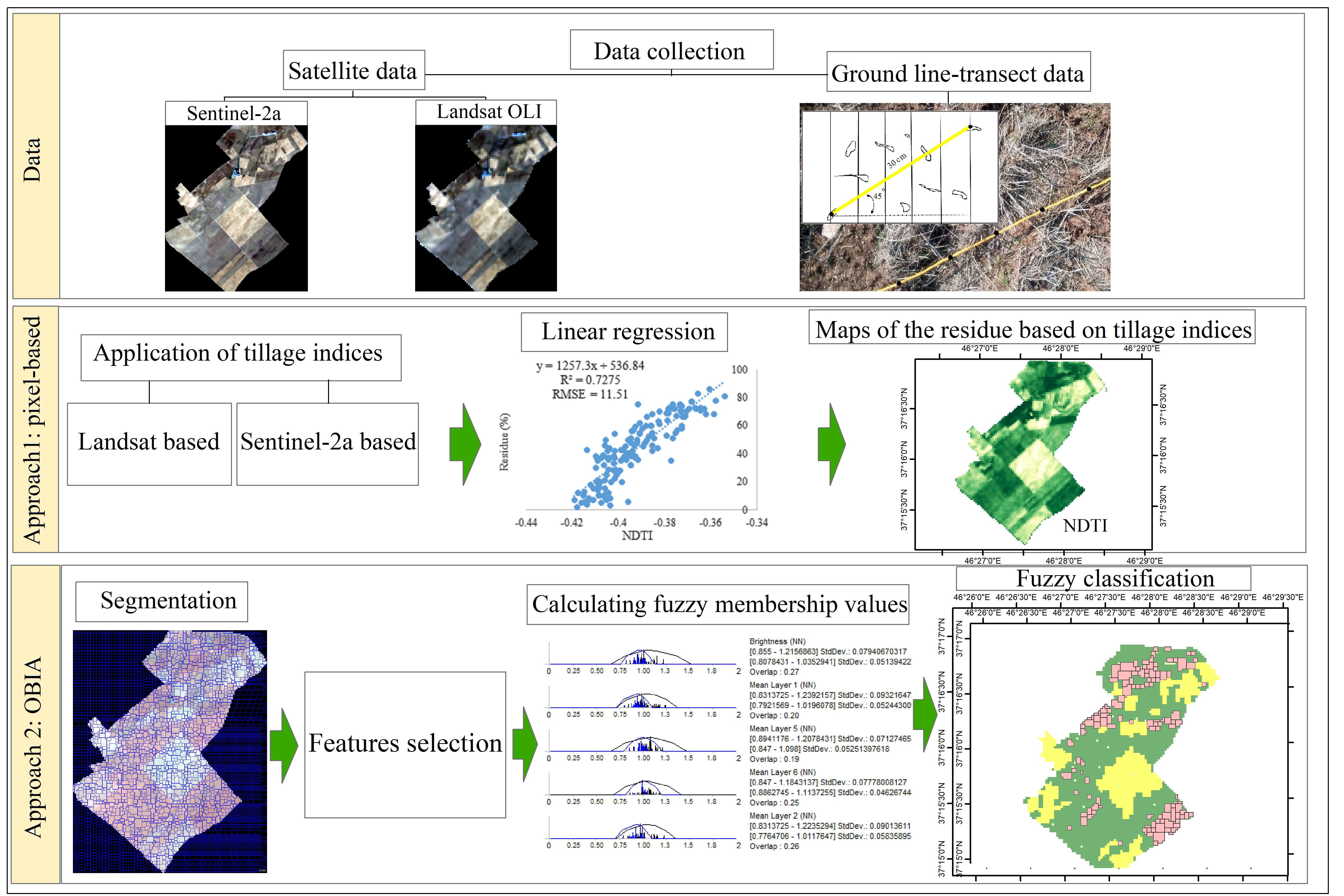
Between 5 and 15 October 2017, the SSR was measured at the experimental fields of the study area through line transects. First, we used a 30 m measuring rope, which was divided into 100, 30 cm intervals shown as black markings. At each sampling location, the rope was stretched diagonally (45°) across the rows and the number of markings intersecting the SSR was counted. Then we stretched the rope across the rows again, but in the direction perpendicular to the first mode. After that, the percentage of the SSR was calculated by taking the average number of markings of the two counting exercises. The exact location of each SSR location was obtained by a global positioning system (GPS) measurement in the field. A total of 153 local points was measured with this line transect method over the study area of 450 hectares.

2.3. Remote Sensing Data

Two sources of satellite images were utilized in this study, namely Sentinel-2A and Landsat-8. A Sentinel-2A image from 9 October 2017 and a Landsat-8 image from 16 October 2017 were acquired. We used the ENVI 5.3 software for all image preprocessing tasks, including radiometric and atmospheric corrections. We selected bands 2, 3, 4, 5, 6, and 7 of the Landsat-8 image with a resolution of 30 m and used these bands together with bands 5, 6, 7, 8a, 11, and 12 of the Sentinel-2A image, whereby the latter has a spatial resolution of 20 m. The two images were preprocessed using the ENVI 5.3 software.

2.4. Soil Surface Residue Identification: Workflow

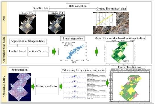
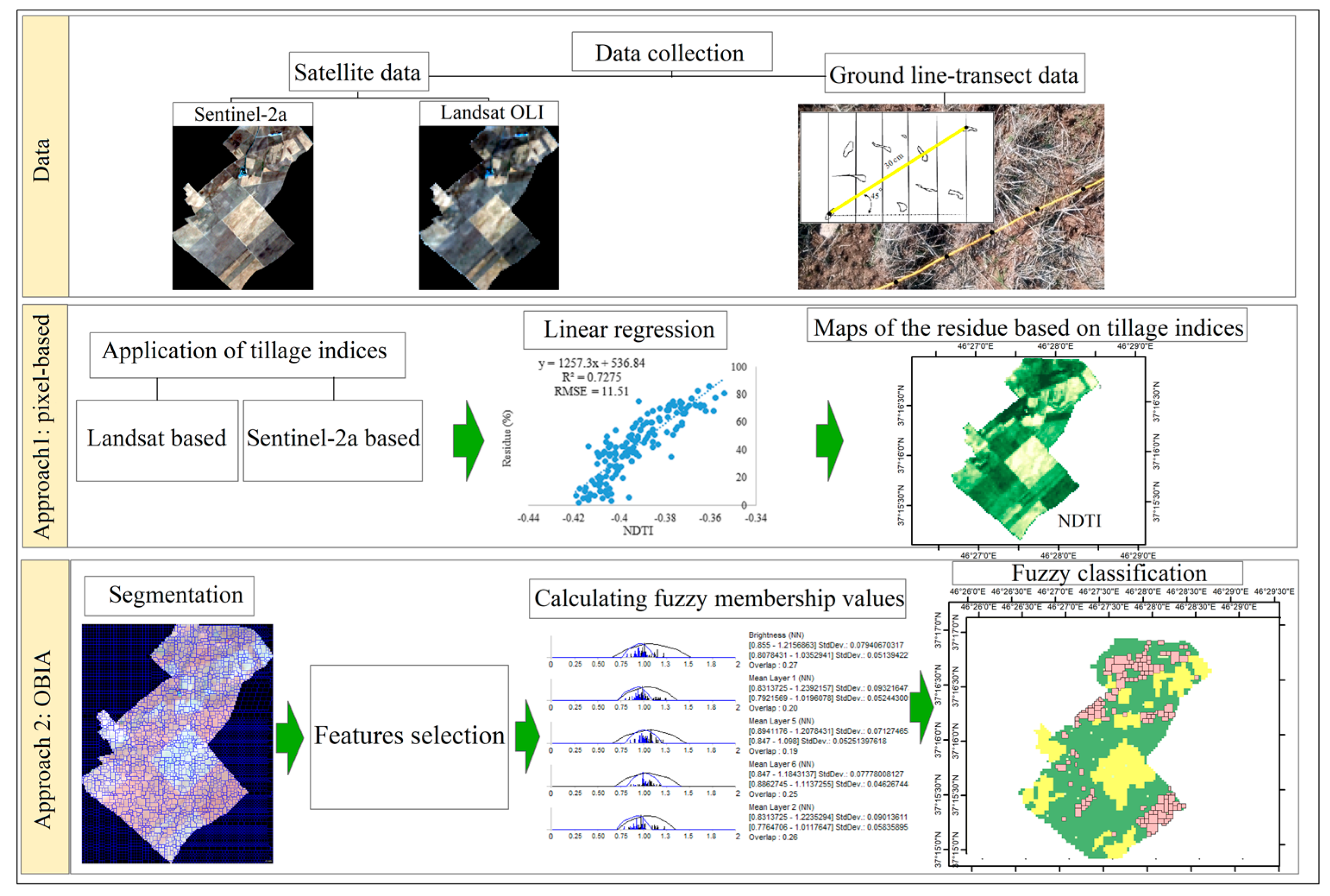
For the Landsat-8 and Sentinel-2A data, two different approaches were applied to map the SSR (Figure 2), namely, a) a common per-pixel method, which relies on the linear regression between tillage indices and line transect field measurements and b) a classification based on fuzzy OBIA methods. In general, a pixel-based approach estimates the residue cover continuously using tillage indices. However, the OBIA method classifies the residue cover at different levels. While, both the methods have some advantages in terms of estimation of the residue, because the final objective is to determine the applied tillage methods in a region (depending on the percentage of residue cover that is left on the field after tillage and planting practices), object-based classification methods are discussed in particular in this study.

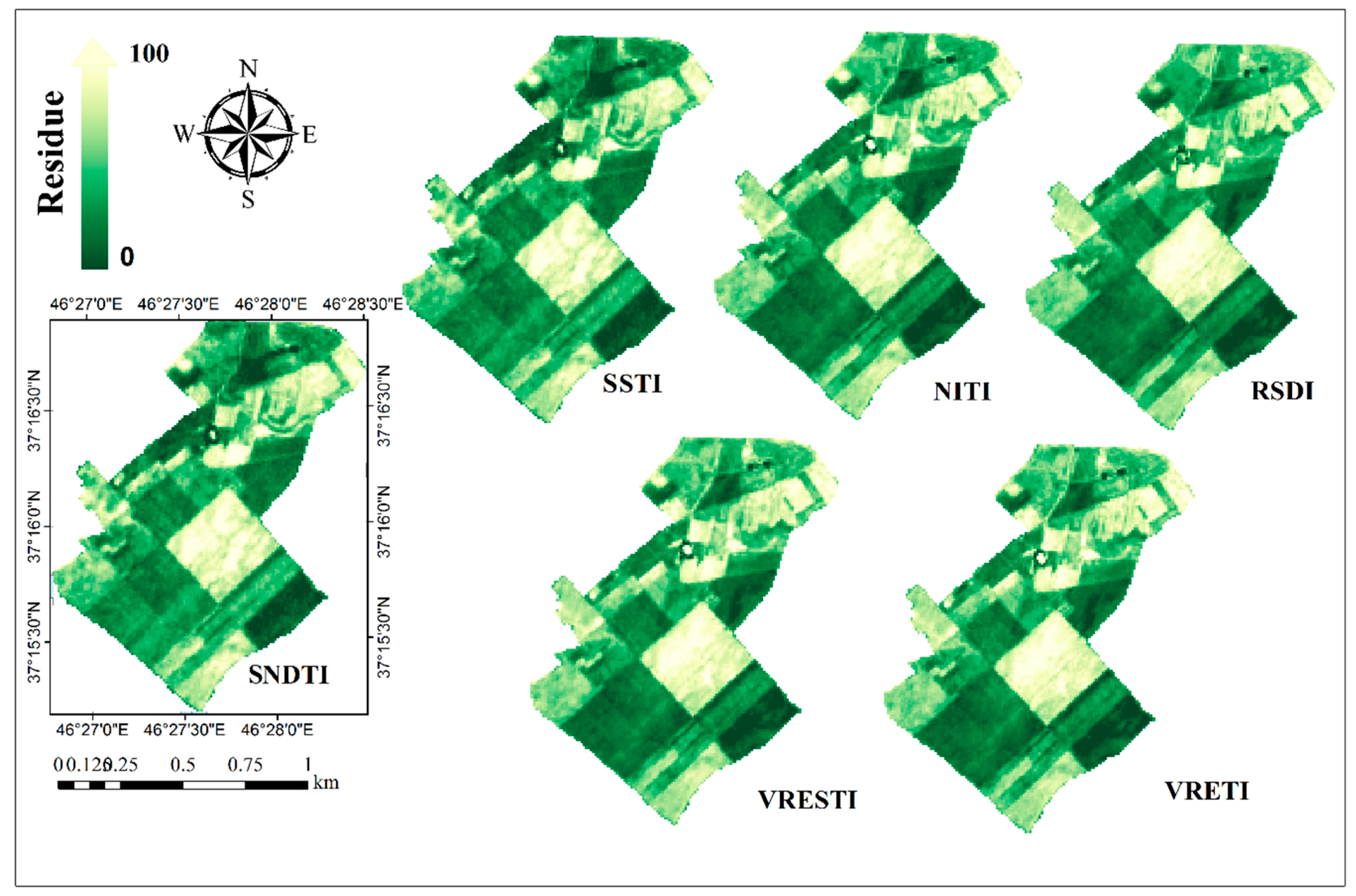
2.5. Tillage Indices

The spectral specifications of Sentinel-2A and Landsat-8 images are shown in

Table 1. Specifications of Sentinel-2A and Landsat-8 satellite images (in bold: bands used in this study).

Sentinel-2A			Landsat-8
Band Specification	Wavelength (nm)	Resolution (m)	Band Specification	Wavelength (nm)	Resolution (m)
Band 1—Coastal	433–453	60	Band 1—Coastal	433–453	30
Band 2—Blue	458–523	10	Band 2—Blue	450–515	30
Band 3—Green	543–578	10	Band 3—Green	525–600	30
Band 4—Red	650–680	10	Band 4—Red	630–680	30
Band 5—Vegetation red edge	698–713	20	Band 5—NIR	845–885	30
Band 6—Vegetation red edge	734–748	20	Band 6—SWIR	1560–1660	30
Band 7—Vegetation red edge	765–785	20	Band 7—SWIR	2100–2300	30
Band 8—NIR	785–900	10	Band 8—Panchromatic	500–680	15
Band 8a—Vegetation red edge	855–875	20	Band 9—Cirrus	1360–1390	30
Band 9—Water vapor	930–950	60	Band 10—Thermal	10,600–11,200	100
Band 10—SWIR—Cirrus	1365–1385	60	Band 11—Thermal	11,500–12,500	100
Band 11—SWIR	1565–1655	20
Band 12—SWIR	2100–2280	20

. As described in Section 3.2, we only used six bands from each satellite to map the residue.

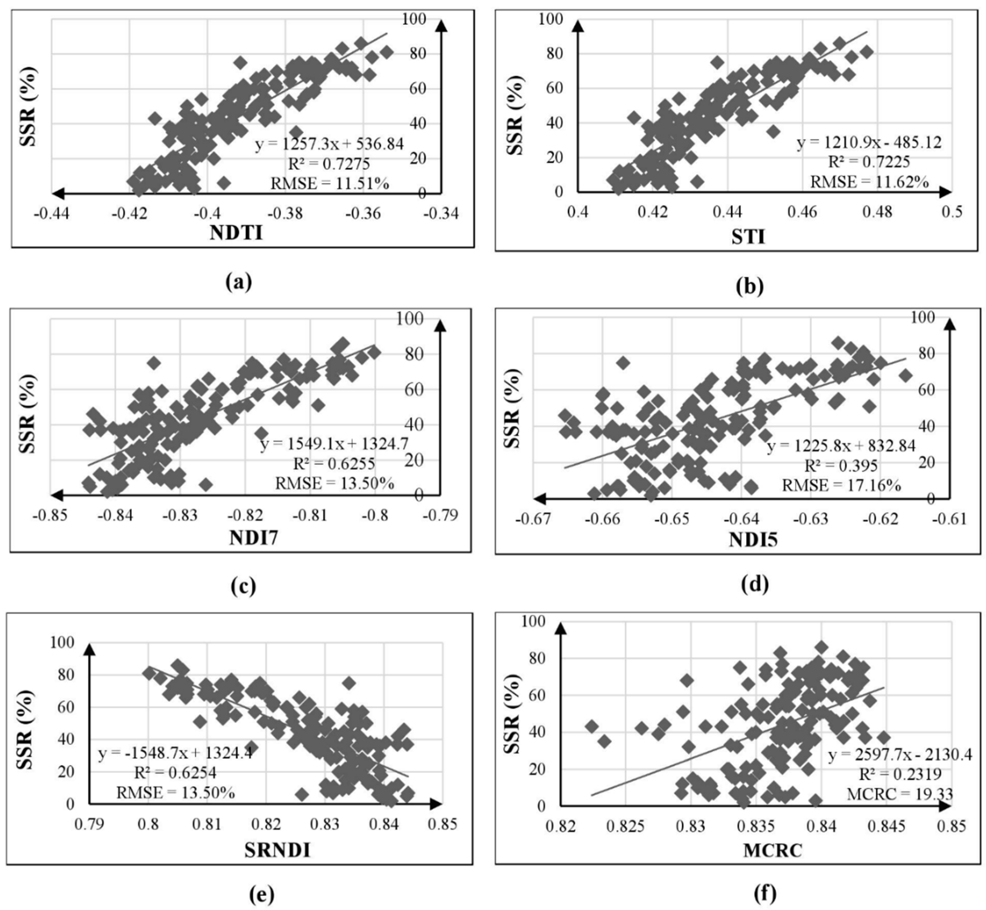
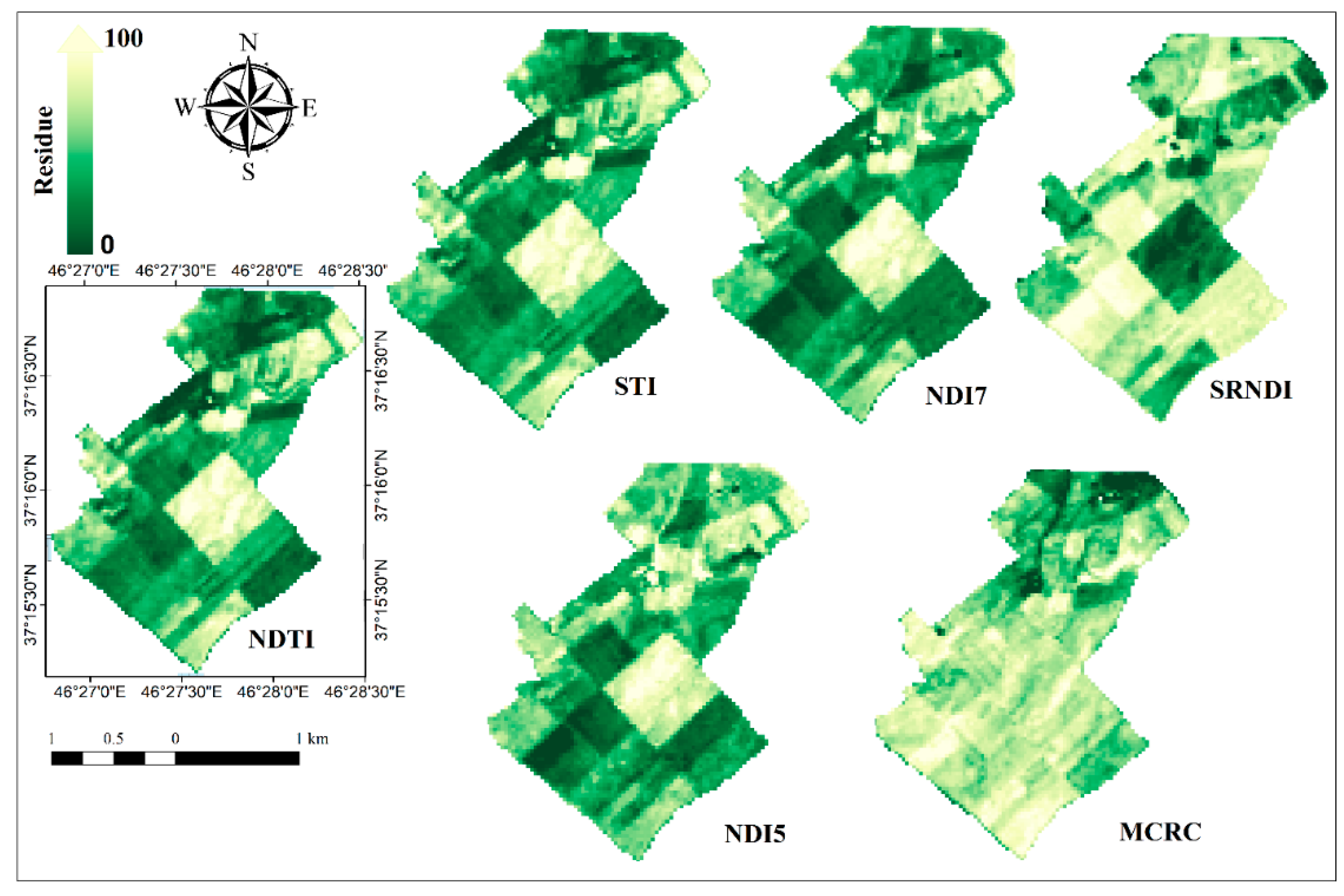
To calculate the relationship between spectral properties and residue cover, two categories of indices were considered for Landsat-8 (

Table 2. Landsat-8-based tillage indices.

Index	Formula	Descriptions
NDTI	(B6 − B7)/(B6 + B7)	B3, B4, B5, B6, and B7: Landsat-8 bands of 3, 4, 5, 6, and 7
STI	B6/B7
Modified crop residue cover (MCRC)	(B6 − B3)/(B6 + B3)
Normalized difference index 5 (NDI5)	(B5 − B6)/(B5 + B6)
Normalized difference index 7 (NDI7)	(B5 − B7)/(B5 + B7)
Shortwave red normalized difference index (SRNDI)	(B7 − B4)/(B7 + B4)

) based on the results of the literature review, and comparable indices were developed for Sentinel-2A (

Table 3. Sentinel-2A-based tillage indices.

Index	Formula	Description
SNDTI	(B11 − B12)/(B11 + B12)	B5, B6, B7, B8a, B11, and B12 refer to the respective bands 5, 6, 7, 8a, 11, and 12 of the Sentinel-2A satellite
SSTI	B11/B12
Vegetation red edge shortwave tillage index (VRESTI)	(B7 − B12)/(B7 + B12)
Narrow near-infrared tillage index (NITI)	(B8a − B12)/(B8a + B12)
Vegetation red edge tillage index (VRETI)	(B6 − B12)/(B6 + B12)
Red shortwave difference index (RSDI)	(B5 − B12)/(B5 + B12)

).

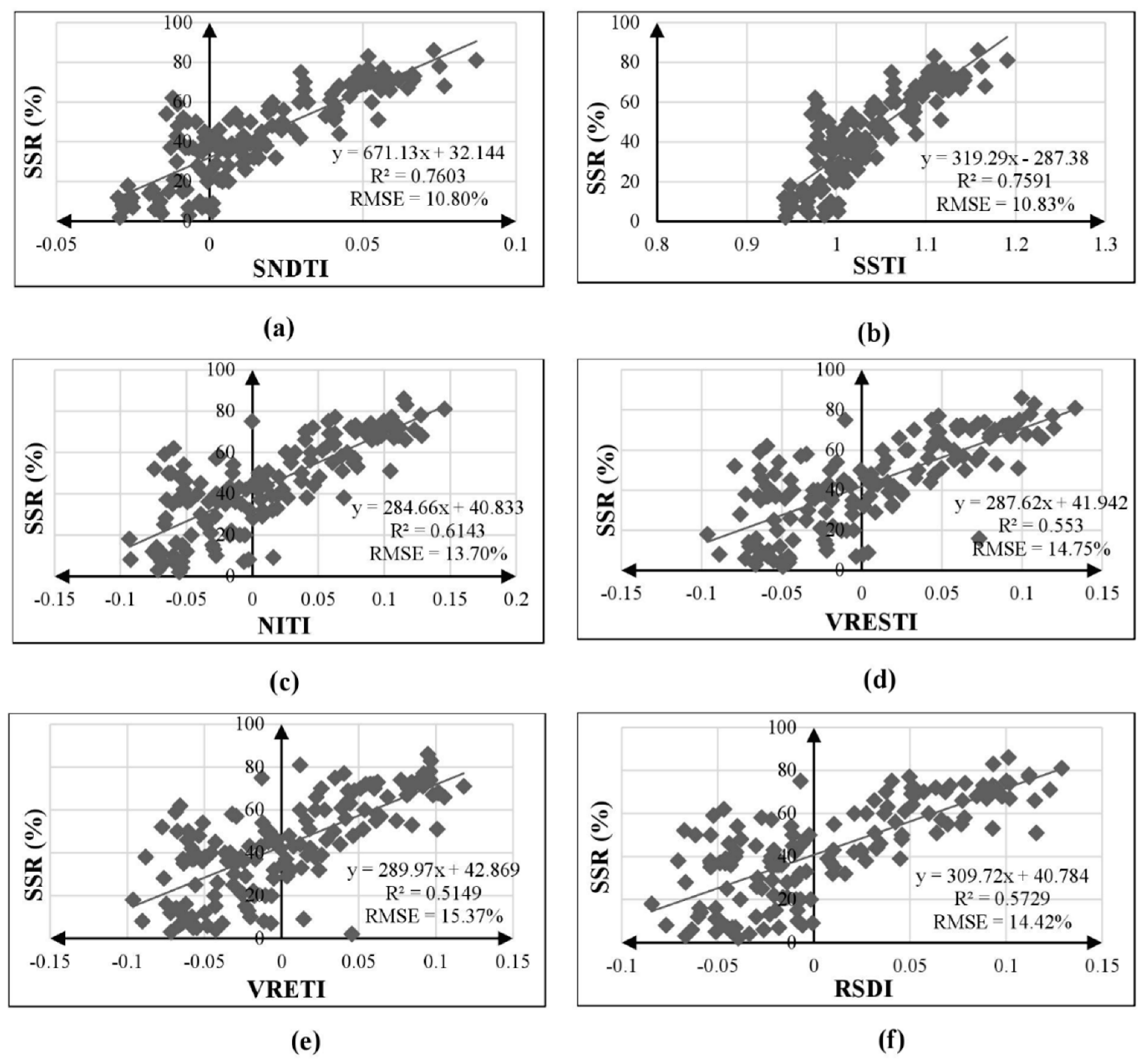
Due to the wavelength similarities of Landsat-8 bands 6 and 7 and Sentinel-2A bands 11 and 12, we created similar indices for Sentinel-2A images as Sentinel NDTI (SNDTI) and Sentinel STI (SSTI).

2.6. Object-Based Image Analysis

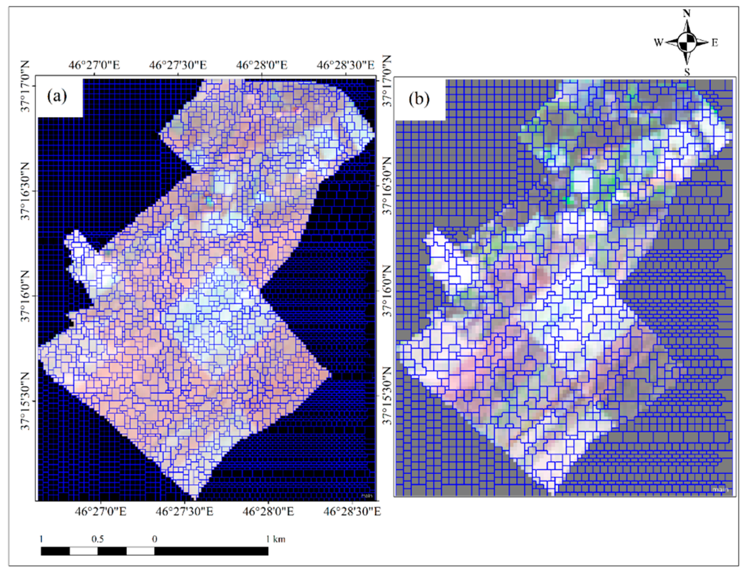
2.6.1. Image Segmentation

Image segmentation is typically the first step in an OBIA workflow. It clusters relatively homogenous pixels into objects [42,43,44]. Multi-resolution segmentation is the most common image segmentation process in OBIA and it serves the objective to derive “relatively homogeneous regions” by a global optimization heuristic [42]. It is a bottom-up region-merging algorithm that merges adjacent pixels with similar specifications to create initial image objects. It then merges similar objects together to produce larger objects. This is carried out as long as the internal heterogeneity (color, texture, and shape) of produced objects does not exceed user-defined thresholds [37,42,45,46,47,48].

These multi-resolution segmentation processes usually apply the three parameters of scale, color, and shape. The scale parameter value is not equal to the sizes of the resulting objects, but strongly influences their sizes. A high scale parameter value allows for a high heterogeneity within image objects and tends to result in larger segments. Likewise, a low scale parameter value results in a high homogeneity within image objects and a smaller number of image objects [28,44,49]. Drǎguţ et al. [47] developed methods for estimating appropriate scale parameters prior to the segmentation step. Shape and color are additional parameters in multi-resolution segmentation that influence spectral and textural homogeneity of the image objects, while shape influences the resulting objects in terms of their smoothness and compactness. Based on the method of Drǎguţ et al. and initial trials, we used color and shape parameters of 0.4 and 0.5, respectively, for Landsat-8 and Sentinel-2A images. The segmentation processes are illustrated in Figure 3.

2.6.2. Basic Fuzzy Concepts Used in OBIA

In mathematics, two general logics are distinguished, namely, binary and fuzzy. While binary is a two-valued logic that considers only $\left\{0, 1\right\}$ for each object, fuzzy is a multi-valued logic that considers [0,1] for each member. The fuzzy set theory was introduced by Zadeh [50] to investigate uncertainty using linguistic terms instead of common numerical variables. As discussed in the literature review, most OBIA studies use fuzzy rule-based classifications and employ either membership functions or a nearest neighbor classifier (for differences and advantages of both methods, see [51]).

In a fuzzy object-based image analysis procedure, the characteristics of each image object can be qualified by a fuzzy feature space and described by a membership function. A fuzzy rule is a set of orders that makes a correspondence relationship between the features that describe each object and the class.

Membership Function Method

Membership functions assign fuzzy values to a predefined feature space for each object class using a particular membership function (larger than, smaller than, singleton, Gaussian, about range, and full range) [29,36,46]. Features with high membership values (depending on the test conditions) are selected for classification [33,52,53]. The classification operator is another important factor that affects classification accuracy since it determines how several rules are combined. The most frequently used operators are simple ‘AND’ and ‘OR’ functions, but more complex operators can also be defined.

In the present study, the membership function method is applied to both Landsat-8 and Sentinel-2A images through the following steps: a) determining the number of classes, b) selecting feature space(s), c) calculating fuzzy membership values for each object class, and d) applying the classification algorithm.

Basic Concepts of NN

Classifiers are often grouped into the following: (i) parametric classifiers that require a learning/training phase of the classifier parameters, these methods are also known as learning-based approaches, and (ii) nonparametric classifiers, which is a group of classifiers that require no learning/training phase for the determination of classifier parameters [54]. Classification decision in nonparametric classifiers is directly based on the data. In object-based image analysis, NN is a popular nonparametric classifier that relies on estimating the NN distance from the nearest (most similar) image objects in the database. There are several advantages to using nonparametric classifiers compared to parametric methods, in particular, that a) a learning/training phase is not required, and b) nonparametric classifiers can easily handle a large number of classes. Parametric classifiers require training of parameters which may take several days for large dynamic databases, while for nonparametric classifiers changing classes/training sets is straightforward [55]. In addition, to validate the results, NN classifiers provide almost unlimited capabilities for a classification system, which can be extended to other areas by selecting training samples [54]. The NN method in this study consists of the following three main steps [56]: a) determining the features space, b) training the system with line transect field measurements, and c) applying the classification algorithm.

2.7. Classes and Features Space

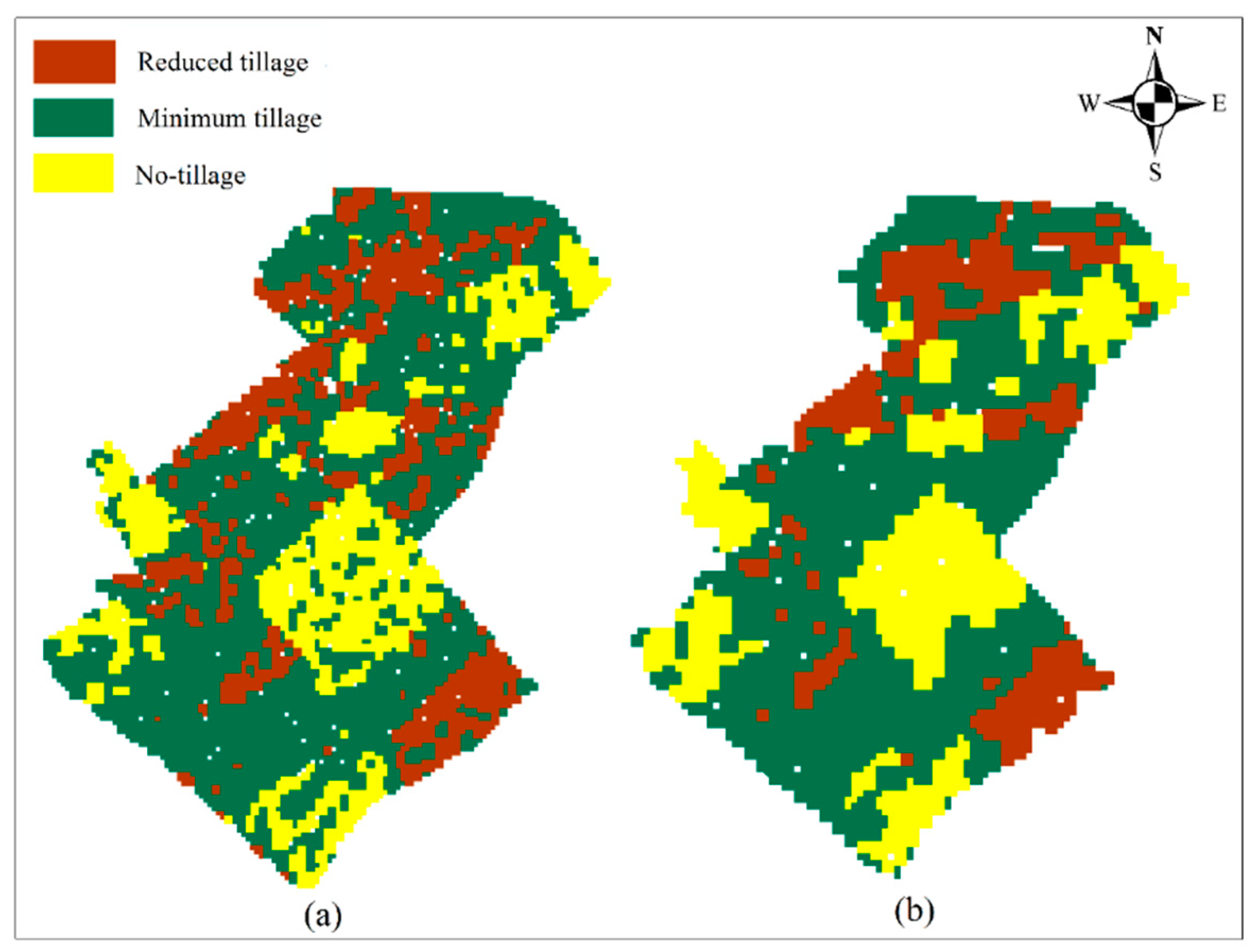
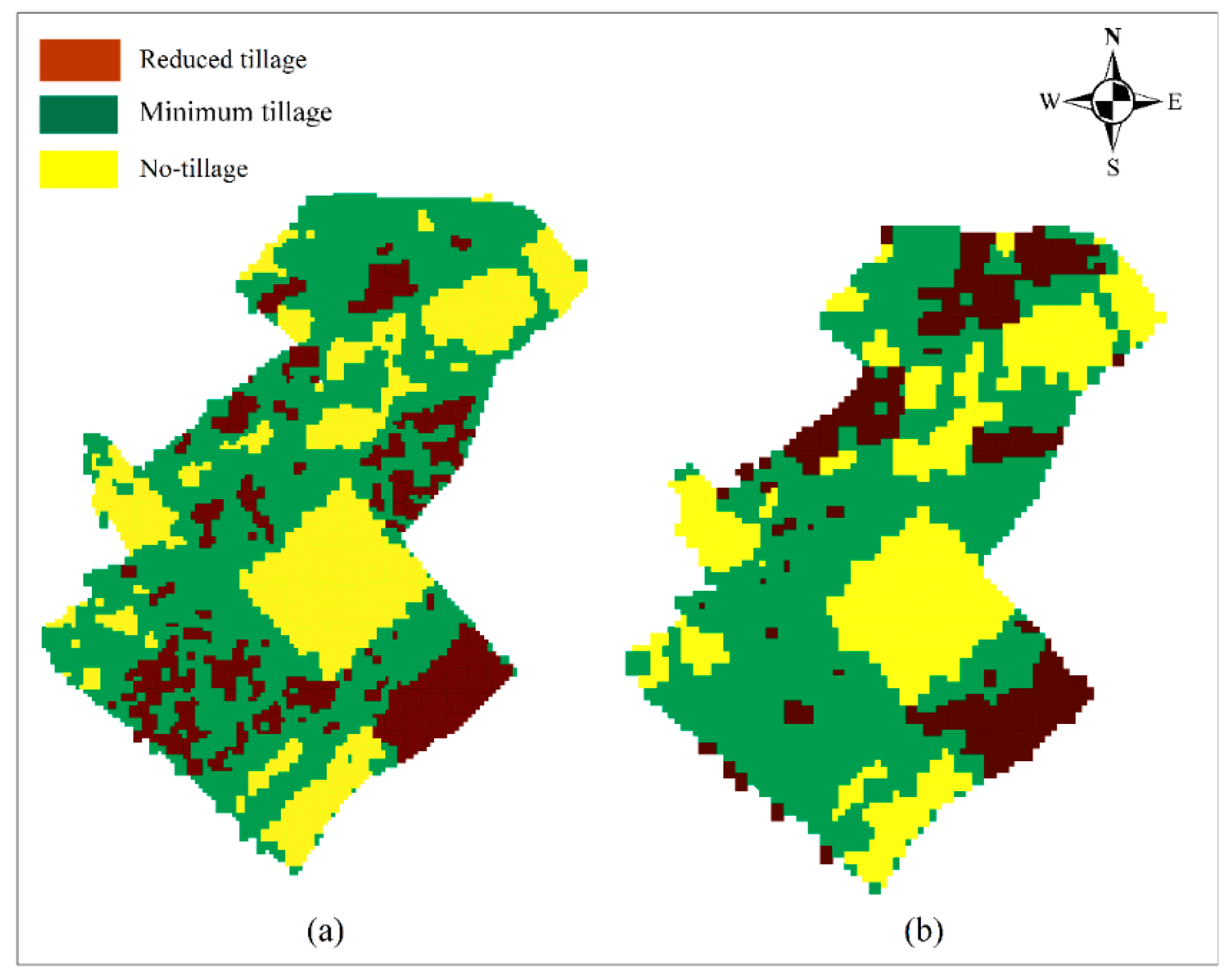
For the classification of SSR and tillage intensity, three classes were considered in this study: SSR < 30% (reduced tillage), SSR 30%–60% (minimum tillage), and SSR > 60% (no tillage). Three different groups of features, namely, mean features, tillage features, and GLCM textural features, were applied to both the methods, membership functions, and NN. The features were selected based on the results of the literature review.

2.7.1. Mean Features

In this study, band ratio, brightness, and maximum difference (Max. Diff) were considered as the mean functions for both Sentinel-2A and Landsat-8 data. The band ratio included bands 2, 3, 4, 5, 6, and 7 of Landsat-8 data with a resolution of 30 m and bands of 5, 6, 7, 8a, 11, 12 of Sentinel-2A data with a resolution of 20 m. The brightness of an object represents the quality of lightness or darkness within each image object [41,57,58]. Due to the contrast between soil and residue, lightness or darkness within an object may differ from one to another. Accordingly, increasing the SSR within an object increases the brightness of the object while an increasing amount of soil within an object decreases the brightness of the object.

$$B=\frac{ {{\displaystyle \sum }}_{i=1}^{n_{vis}}{\overline{c}}_{i\left(vis\right)}}{n_{vis}},$$

(1)

where B is the brightness of an image object, ${\overline{c}}_{i\left(vis\right)}$ is the sum of the mean object brightness in the visible bands, and $n_{vis}$ is the number of corresponding spectral bands.

In OBIA, Max. Diff (MD) for each image object is defined as the absolute difference between the minimum object mean and the maximum object mean in the visible bands divided by the mean object brightness [37].

$$MD=\frac{ \left|min\left({\overline{C}}_{i\left(vis\right)}\right)-max\left({\overline{C}}_{i\left(vis\right)}\right)\right|}{B},$$

(2)

2.7.2. Tillage Features

In the literature review, we discussed different tillage spectral indices which aim to distinguish the SSR from soil. These indices might vary depending on the type of spectral image (multispectral and hyper-spectral) and the characteristics of the sensor. We used the indices described in Section 3.2 and Table 2 and Table 3.

2.7.3. Textural Features

Textural features based on a gray level co-occurrence matrix (GLCM) were first introduced by Haralick et al. [59]. The initial 23 textural features were decreased to eight major features (

Table 4. Gray level co-occurance matrix (GLCM)-based textural features

Index	Formula
Angular second moment (ASM)	${{\displaystyle \sum }}_i{{\displaystyle \sum }}_j{\left\{p\left(i,j\right)\right\}}^2$
Contrast	${\displaystyle \sum _{i,j=0}^{N-1}}{p}_{i,j}{\left(i-j\right)}^2$
Correlation	${\displaystyle \sum _{i,j=0}^{N-1}}{p}_{i,j} \left[\frac{\left(i-{\mu }_i\right)\left(j-{\mu }_i\right)}{\sqrt{\left({\sigma }_i^2\right)\left({\sigma }_j^2\right)}}\right]$
Dissimilarity	${\displaystyle \sum _{n=0}^{N-1}}n\left\{{\displaystyle \sum _{i=1}^N}{\displaystyle \sum _{j=1}^N}p\left(i,j\right)\right\}$
Entropy	${\displaystyle \sum _{i,j=0}^{N-1}}{p}_{i,j} \left(-ln p_{i,j}\right)$
Homogeneity	${{\displaystyle \sum }}_i{{\displaystyle \sum }}_j\frac{1}{1+{\left(i-j\right)}^2}p\left(i,j\right)$
Mean	${\mu }_i={\displaystyle \sum _{i,j=0}^{N-1}}i\left(p_{i,j}\right) { }^{ }$
Standard Deviation (St.D)	${\sigma }_i=\sqrt{{\displaystyle \sum _{i,j=0}^{N-1}}{p}_{i,j}\left(i,j-\frac{{{\displaystyle \sum }}_{i,j=0}^{N-1}{p}_{i,j}}{N^2}\right) }$

) in [60]. Textural features are calculated based on the distance and angle between two pairs of adjacent pixels that are located in a window. The accurate extraction of textural features in a pixel-based image analysis method depends on the size of the window, while in an object-based approach, the results of segmentation create objects with different shapes and sizes. These objects, which are considered as windows, can illustrate the real shape and size of the land cover objects [61].

The main assumption in the computation of object-based GLCM textural features is the probability of the simultaneous presence of a pair of objects with the same brightness. The GLCM is a square matrix in which each member represents the number of pairs of pixels. The GLCM texture considers the relationship between two pixels at a time. These two pixels are called the reference and neighbor pixels and they are at a distance d and an angle θ to each other [62]. The directions of analysis for GLCM can be horizontal (0°), vertical (90°), or diagonal (45° and 135°) and are denoted as $a_0$, $a_{45}$, $a_{90}$, and $a_{135}$.

2.8. Accuracy Assessment

2.8.1. Overall Accuracy

The estimation of the error matrix is the most common method for estimating the accuracy of the classification results. To analyze the classification quality, the error matrix compares the classification results with ground truth data. The overall accuracy is the key factor to evaluate the accuracy of the classified map. It can be calculated as the area of the correctly classified sample objects divided by the total area of sample objects (Equation (3)) [27].

$$OA= \frac{{{\displaystyle \sum }}_{k=1}^N{a}_{kk}}{{{\displaystyle \sum }}_{i,k=1}^N{a}_{ik}},$$

(3)

where i is the row number, j is the column number, $p\left(i,j\right)$ is normalized value in the cell, and N is the number of rows or columns.

2.8.2. User Accuracy

The user accuracy is the accuracy from the point of view of a map user. It demonstrates how the class on the map will actually be present on the ground. The user accuracy is calculated from the number of correctly identified objects in a given map class divided by the number of claimed objects to be in that map class (Equation (4)) [27].

$$UA= \frac{a_{ii}}{{{\displaystyle \sum }}_{i=1}^N{a}_{ik}},$$

(4)

2.8.3. Producer Accuracy

The producer accuracy is the accuracy from the point of view of a map maker. It demonstrates how the real objects on the ground are correctly shown on the classified map. It is also calculated from the number of correctly identified objects in the reference plots of a given class divided by the number actually in that reference class (Equation (5)) [27].

$$PA= \frac{a_{tt}}{{{\displaystyle \sum }}_{i=1}^N{a}_{ki}},$$

(5)

2.8.4. Kappa Statistics

The kappa coefficient is a statistical method that measures the accuracy of an image classification process. The reason for the robustness of this method is that it eliminates agreement occurring by chance through the classification. The range of the kappa coefficient is from −1 to 1. A value of 1 indicates that the raters are in complete agreement [63]. A value of 0 indicates no agreement between the raters, which means the classification is completely by chance. A negative kappa coefficient indicates agreement worse than occurring by chance. The kappa coefficient is expressed as:

$$\kappa =\frac{P_a-P_e}{1-P_e},$$

(6)

where $P_a$ is the probability of relative observed agreement between raters and $P_e$ is the probability of a chance agreement.

3. Results

3.1. Tillage Indices

The spectral indices described in Section 2.5 were calculated to estimate the residue. Figure 4 shows the linear correlation between Landsat-8-based tillage indices (normalized difference tillage index (NDTI), simple tillage index (STI), normalized difference index 7 (NDI7), normalized difference index 5 (NDI5), shortwave red normalized difference index (SRNDI), and modified crop residue cover (MCRC)) and the percentage of the SSR.

The coefficient of determination ($R^2$) explains how much a dependent variable (here, surface residue) is affected by an independent variable (here, tillage indices) and to what degree these changes are impacted by related objects such as soil and vegetation. The root-mean-square error (RMSE) also indicates the distance of the individual points from a regression line, whereby greater distances mean greater errors and lower distances are equal to smaller errors.

The linear regression between the Landsat indices and SSR demonstrated NDTI as the best index with $R^2$ of 0.727 and RMSE of 11.51%, closely followed by the STI with $R^2$ of 0.722 and RMSE of 11.62%. Thus, both NDTI and STI are efficient SSR estimators, which is in line with the results of earlier studies (e.g., [12,16,18,21,22]). The NDI7 and SRNDI indices yielded similar results with $R^2$ and RMSE values of 0.625 and 13.50%, respectively. Finally, the results of NDI5 and MCRC were considered to be insufficient with $R^2$ of 0.395 and 0.232 and RMSE of 17.16% and 19.33%, respectively. This is again in line with the results of Sullivan et al. [64].

As mentioned in the literature review, lignin and cellulose in the residue cause a high absorption at the electromagnetic spectra around 2100 nm wavelength. The NDTI and STI utilize Landsat-8 bands 6 and 7 which cover wavelengths between 1560 nm and 2300 nm. Once the wavelength range is too broad, other factors such as water, vegetation, soil, and minerals may influence the results. Figure 5 shows an SSR map of the Landsat-8-based indices. Brighter regions indicate more residue on the surface and darker areas represent a shortage of the SSR.

In a second step, the Sentinel-2A satellite image (bands 5, 6, 7, 8a, 11 and 12) with 20 m resolution was similarly investigated to estimate the percentage of the SSR (Figure 6).

The SNDTI-based model correlates with the ground truth data with $R^2$ of 0.76 and RMSE of 10.80%, followed by the SSTI indicator with $R^2$ of 0.75 and RMSE of 10.83%. The Narrow near infrared tillage index (NITI) indicator yielded $R^2$ of 0.61 and RMSE of 13.67%. Figure 7 shows the resulting SSR maps based on the Sentinel-2A satellite image data. Lighter areas indicate high SSR values and darker regions represent low SSR values.

3.2. Results of Object-Based Image Analysis Methods

3.2.1. Fuzzy Object-Based Image Analysis

Fuzzy Membership Values

According to our literature review, the fuzzy sigmoid function was described as a very suitable function to compute fuzzy membership values of feature spaces in several studies. Thus, we computed fuzzy membership values using a Gaussian function. Results are presented in

Table 5. Membership values of feature spaces for the Sentinel-2A and Landsat-8 images.

Sentinel-2A				Landsat 8
Features	Membership Values			Features	Membership Values
	<30%	30%–60%	>60%		<30%	30%–60%	>60%
VRETI	0.846	0.922	0.907	NDVI	0.862	0.917	0.973
RSDI	0.842	0.903	0.878	NDSVI	0.962	0.958	0.844
SNDTI	0.939	0.922	0.965	SRNDI	0.963	0.893	0.885
SSTI	0.937	0.925	0.962	NDI7	0.981	0.902	0.839
NITI	0.873	0.917	0.920	NDI5	0.943	0.813	0.77
VRESTI	0.849	0.926	0.914	MSSR	1	0.95	0.928
Entropy	0.826	0.815	0.753	STI	0.979	0.978	0.893
Dissimilarity	0.825	0.918	0.824	NDTI	0.976	0.967	0.914
Homogeneity	0.760	0.961	0.882	Homogeneity	0.93	0.955	0.942
ASM	0.848	0.858	0.900	Contrast	0.97	0.85	0.69
Contrast	0.902	0.912	0.898	St. D	0.977	0.683	0.636
St. D	0.923	0.866	0.905	ASM	0.924	0.867	0.806
Mean	0.931	0.902	0.991	Dissimilarity	0.97	0.862	0.75
Correlation	0.995	0.969	0.935	Mean	0.637	0.993	0.879
Band 6	0.884	0.867	0.882	Entropy	0.893	0.878	0.839
Band 7	0.871	0.858	0.876	Correlation	0.914	0.793	0.674
Band 8a	0.882	0.853	0.879	Max. Diff	0.963	0.902	0.846
Band 11	0.958	0.926	0.953	Band 2	0.994	0.941	0.948
Band 12	0.98	0.956	0.979	Band 4	0.99	0.966	0.985
Band 5	0.853	0.865	0.863	Band 5	0.948	0.911	0.972
Max. Diff	0.86	0.948	0.926	Band 3	0.964	0.97	0.997
Brightness	0.888	0.872	0.917	Band 7	0.967	0.985	0.751
				Band 6	0.987	0.997	0.919
				Brightness	0.973	0.998	0.886

and the functions with the highest membership values are highlighted in bold.

Results of Classification Based on Fuzzy Membership Functions

We implemented the classification algorithms using eCognition Developer to apply fuzzy logic to membership functions and classified image objects using three classes (Figure 8). The classification algorithm evaluated the class descriptions completely and then assigned each object to the corresponding class.

Accuracy Assessment for the Membership Function Classification

An accuracy assessment was carried out by comparing the map derived using the membership function method with the ground truth data. Results for both Sentinel-2A and Landsat-8 image are shown in

Table 6. Accuracy assessment of object-based image analysis (OBIA) membership function classification for Landsat-8 and Sentinel-2 images.

Sensors	Tillage Methods	Producer Ccuracy	User Accuracy	Kappa Per Class	Overall Accuracy	Overall Kappa
Landsat-8	Reduced tillage	0.928	0.915	0.919	0.924	0.870
	Minimum tillage	0.871	0.920	0.802
	No tillage	0.961	0.928	0.932
Sentinel-2A	Reduced tillage	0.934	0.989	0.915	0.948	0.918
	Minimum tillage	0.879	0.877	0.853
	No tillage	0.954	0.998	0.976

.

3.2.2. Nearest Neighbor Object-Based Image Analysis

Classification of NN Using OBIA

As previously mentioned, the NN classification was applied based on OBIA features. We employed algorithms based on earlier research [28], as well as on results of the per-pixel analysis which is discussed in Section 3.1. We employed three groups of features for the Landsat-8 image, namely a) spectral features (mean values for bands 4, 5, and brightness), b) textural features (GLCM mean), and c) tillage features (NDTI, STI, and NDI7). Likewise, we employed the same spectral features, textural features, and the new tillage features (SNDTI, SSTI, and NITI) for the NN classification of the Sentinel-2A image. Figure 9 shows the results of the NN classification for object-based SSR mapping.

Accuracy assessment of NN-OBIA

An accuracy assessment was carried out by comparing the map created using the NN method with a reference map based on validated ground truth data. Results for both Sentinel-2A and Landsat-8 data are shown in

Table 7. Accuracy assessment of the NN classification method using OBIA for Landsat-8 and Sentinel-2A images.

Sensors	Tillage Methods	Producer Accuracy	User Accuracy	Kappa Per Class	Overall Accuracy	Overall Kappa
Landsat-8	Reduced tillage	0.693	0.571	0.525	0.812	0.734
	Minimum tillage	0.654	0.743	0.828
	No tillage	0.840	0.982	0.761
Sentinel-2A	Reduced tillage	0.921	0.834	0.705	0.891	0.813
	Minimum tillage	0.853	0.882	0.787
	No tillage	0.949	0.894	0.820

.

4. Discussions

Some earlier remote sensing-based studies demonstrated the potential to distinguish no tillage from intensive tillage, but it was and is still difficult to distinguish between categories of conservation tillage (minimum tillage and no tillage) due to the similarities between soil and residue [21,65]. The present study employed per-pixel and object-based image analysis approaches to estimate the SSR using Sentinel-2A and Landsat-8 data.

4.1. Landsat-8 vs. Sentinel-2A

We aimed to compare the capability of Sentinel-2A and Landsat 8 satellite images for SSR mapping. Different band combinations were employed to explore the capabilities of six Sentinel-2A bands for analyzing the SSR using six Sentinel-2A bands (5, 6, 7, 8a, 11, and 12). In order to map the SSR from Sentinel-2A, we developed the following indices: Sentinel normalized difference tillage index (SNDTI), Sentinel simple tillage index (SSTI), narrow near infrared tillage index (NITI), vegetation red edge shortwave tillage index (VRESTI), red shortwave difference index (RSDI), and vegetation red edge tillage index (VRETI). The same bands and indices were applied to per-pixel and OBIA image analysis methods. The results of estimating the SSR using Landsat-8 and Sentinel-2A data models revealed that Sentinel-2A indices (Sentinel NDTI and Sentinel STI) were able to map the SSR more efficiently than Landsat-8 and its respective indices (Landsat NDTI and Landsat STI). Differences in the spatial resolution of these two major sources of remote sensing data justify such a difference. In particular, Sentinel-2A has a 20 m spatial resolution with 13 bands, while Landsat has a 30 m spatial resolution and 11 bands. Due to the absorption properties of lignin and cellulose at 2100 nm of the electromagnetic spectrum, it can be concluded that both NDTI and STI indicators for Landsat-8, and NDTI and STI indicators for Sentinel-2A, which monitor the spectrum region of 2100 nm, were able to estimate and map the SSR more accurately than other indices. Similar results have also been reported in earlier research using Landsat satellites images [10,12,17,19].

4.2. Pixel-Based Image Analysis

As demonstrated in Section 3, per-pixel approaches for Landsat-8 satellite images using NDTI and STI indices yielded R² values of 0.727 and 0.722, respectively. Sentinel-2a and the novel but comparable indices yielded R² values of 0.760 and 0.759, respectively. It means that the Sentinel-2 data better matched the ground truth data. Due to the same spectral resolution for the applied bands (1560–1660 nm and 2100–2300 nm) for those indices, and given that all the images were subjected to the same radiometric and atmospheric corrections, it is concluded that the spatial resolution of Sentinel-2 data improved the correlation of estimated SSR data with the ground truth data. It was also a key factor for producing lower RMSE than Landsat 8 data.

Results showed that, while getting closer to the 2100 nm region in the selection of bandwidths for calculating an indicator, increased the correlation between estimated and actual SSR and produced higher RMSE, getting away from that region produced lower RMSE. It obviously can be observed for NDI7 (band 5–band 7), SRNDI (band 7–band 4), NDI5 (band 5–band 6), and MCRC (band 6-band 3) for Landsat-8 indices and NITI (band 8a–band 12), VRESTI (band 7–band 12), and VRETI (band 6–band 12) for Sentinel-2 indices. The results were in line with former studies [19,20,22].

4.3. Object-Based Image Analysis

We tested several OBIA methods and achieved very high overall accuracies of up to 0.948 for Sentinel-2A and 0.891 for Landsat-8, but with some differences between the two OBIA approaches used. Earlier studies also yielded high accuracies using Landsat images for SSR classification [21,26]. As discussed in Section 2, the basis for classifying using the OBIA approach is the application of fuzzy logic to assign objects in the scene to each class. In this way, two methods of classification (membership functions and nearest neighbor) were employed. Overall accuracy results in Section 4 showed a fine superiority of membership functions over the nearest neighbor. The most important reason that can influence this superiority is the applied method for selecting properties in order to assign local objects to the classes. While, membership functions perform based on the magnification of the fuzzy number for each object class, in the nearest neighbor the properties ascertain based on a map maker’s knowledge, which may increase the overall error of the classification. However, a reason for the popularity of the nearest neighbor may in some cases be faster computations that reduce time costs, because this method does not require time-consuming fuzzy calculations to select final properties [27,28,36].

4.2.1. Membership Function Method

A critical step when using membership functions in the OBIA process is the selection of a suitable membership function to compute fuzzy membership values. To this end, in order to compute membership values for the selection of the final features for the classification, a Gaussian function was applied in our research. Advantages of the Gaussian functions are that they need less data to define a membership function and that the membership function parameters can easily be modified. In addition, the partition unity condition is automatically satisfied (the sum of the membership values for each object is equal to 1) as discussed in former studies [66,67].

The accuracy of a fuzzy membership function classification can be significantly improved by selecting an appropriate operator. As discussed in Section 3, two categories of operators (simple and weighted) were implemented in the eCognition software to make a fuzzy conjunction, disjunction, or complement in the feature spaces. In this study, based on the results of former research [30,36,68], the fuzzy operator of ‘AND’ was applied to classify image objects. Finally, features were selected in a way to apply the classification based on the maximum membership value for a particular object class.

As previously mentioned in Section 3, the accuracy of classification for each individual class was obtained using user and producer accuracies. It was observed that among the three classes (reduced tillage, minimum tillage, and no-tillage), the highest classification accuracy was assigned to the no-tillage class. It was due to the accumulation of the residue in the local objects that classified as no tillage (SSR more than 60%). In this context, the light and yellowish color of the residue well distinguished them from the soil and increased classification accuracy. In terms of accuracies, reduced tillage was the second class to meet study objectives. In this way, the main part of the assigned objects’ class included the dark and brownish color of the soil that distinguished them from the other objects. In this study, minimum tillage class (SSR between 30%–60%) also obtained lowest producer and user accuracies from both Landsat-8 and Sentinel-2A data. The objects assigned to this class were mainly a uniform mixture of residue and soil. It was clearly due to an overlapping problem of spectral boundaries from reduced tillage and no-tillage classes into this class.

4.2.2. The NN Classification Method

As discussed in Section 2.7, one of the most important steps in the NN classification method is to identify efficient feature space. This is due to the direct implementation of the selected feature space in the classification process. It means that no computational evaluation is performed by the NN method to select features. In this study, the primary feature space was composed of three feature categories (mean features, spectral features, and GLCM textural features). Features were selected and optimized based on the results of our earlier research [28] together with results derived from the per-pixel analysis. The comparison of the resulting accuracies of Landsat-8 and Sentinel-2A images using the NN method demonstrated that spatial resolution is a critical factor for SSR detection. Results from the Sentinel-2A satellite with 20 m resolution yielded a higher accuracy than those derived from Landsat-8 data with 30 m resolution, which is in line with the results of earlier studies [21,24].

5. Conclusions

Due to the water and soil erosion problems affected by agricultural activities, the use of conservation tillage methods has increasingly been recommended in recent years as an appropriate alternative to intensive tillage methods. Conservation tillage methods typically leave the previous crop residues, or parts of it, on the soil surface. It is well demonstrated that this practice can significantly reduce water consumption, especially in arid and semi-arid regions.

Intensive tillage methods with burning or burying previous crop residues are in contrast to sustainable agricultural approaches. Today, conservation tillage methods are widely used, and many equipment (machines, pesticides, and specialists) are provided for. Thus, knowing the percentage of residue on the soil surface in a large agricultural area is very informative for agricultural organizations in planning support programs and providing necessary requirements. In precision farming point of view, satellite images can be used for fast and accurate SSR estimation in order to distinguish conventional and conservation tillage practices on the fields with lower time and labor costs. The aim of this study was to provide a fast, inexpensive, and precise solution to map and characterize the residue left on the soil surface after tillage and planting practices. We have found that satellite remote sensing data can be used to identify areas under conservation tillage from those under intensive tillage methods. To this end, we also designed a novel and successful fuzzy object-based approach to estimate SSR and map tillage intensity and then compared it with per-pixel methods. Results indicated that, in general, the remote sensing-based methods can provide appropriate information on the applied tillage methods to technical experts, farmers, and decision makers to improve conservation management efficiency in a region, but with slightly different results between the methods used.

In total, among the applied approaches (pixel-based and object-based), OBIA due to the capability of SSR classification in individual classes is more applicable for decision makers than pixel-based methods (continuous residue cover mapping). When comparing two different OBIA classification strategies, the membership function classifier yielded the highest accuracies for residue mapping. In terms of the comparison of the two satellites used, we can state that Sentinel-2A data yielded better SSR mapping results for both pixel-based (tillage indices) and object-based (membership functions and NN) approaches compared with Landsat-8 data. It was due to the better spatial resolution of the Sentinel-2 images in which the details were better specified and accuracy increased.

References

1. FAO. How to Feed the World in 2050—High Level Expert Forum, Rome 12–13 October, 2009; Office of the Director, Agricultural Development Economics Division, Economic and Social Development Department: Rome, Italy, 2009. [Google Scholar]
2. Wang, X.B.; Cai, D.X.; Hoogmoed, W.B.; Oenema, O.; Perdok, U.D. Developments in conservation tillage in rain-fed regions of North China. Soil Till. Res. 2007, 93, 239–250. [Google Scholar] [CrossRef]
3. D’Emden, F.H.; Llewellyn, R.S.; Burton, M.P. Factors influencing adoption of conservation tillage in Australian cropping regions. Aust. J. Agric. Resour. Econ. 2008, 52, 169–182. [Google Scholar] [CrossRef] [Green Version]
4. Holland, J.M. The environmental consequences of adopting conservation tillage in Europe: Reviewing the evidence. Agric. Ecosyst. Environ. 2004, 103, 1–25. [Google Scholar] [CrossRef]
5. Kay, B.D.; van den Bygaart, A.J. Conservation tillage and depth stratification of porosity and soil organic matter. Soil Till. Res. 2002, 66, 107–118. [Google Scholar] [CrossRef]
6. Melero, S.; López-Garrido, R.; Murillo, J.M.; Moreno, F. Conservation tillage: Short-and long-term effects on soil carbon fractions and enzymatic activities under Mediterranean conditions. Soil Till. Res. 2009, 104, 292–298. [Google Scholar] [CrossRef]
7. Drury, C.F.; Tan, C.S.; Welacky, T.W.; Oloya, T.O.; Hamill, A.S.; Weaver, S.E. Red clover and tillage influence on soil temperature, water content, and corn emergence. Agron. J. 1999, 91, 101–108. [Google Scholar] [CrossRef]
8. Salem, H.M.; Valero, C.; Muñoz, M.Á.; Rodríguez, M.G.; Silva, L.L. Short-term effects of four tillage practices on soil physical properties, soil water potential, and maize yield. Geoderma 2015, 237, 60–70. [Google Scholar] [CrossRef]
9. CTIC. Tillage Type Definitions. West Lafayette; Conservation Technology Information Center, 3495 Kent Avenue, Suite L100, West Lafayette, Indiana 47906, United States: 2002. Available online: http://www.ctic.purdue.edu/resourcedisplay/322 (accessed on 18 July 2018).
10. Daughtry, C.S.T.; Doraiswamy, P.C.; Hunt, E.R., Jr.; Stern, A.J.; McMurtrey, J.E., III; Prueger, J.H. Remote sensing of crop residue cover and soil tillage intensity. Soil Till. Res. 2006, 91, 101–108. [Google Scholar] [CrossRef]
11. Bannari, A.; Pacheco, A.; Staenz, K.; McNairn, H.; Omari, K. Estimating and mapping crop residues cover on agricultural lands using hyperspectral and IKONOS data. Remote Sens. Environ. 2006, 104, 447–459. [Google Scholar] [CrossRef]
12. Zheng, B.; Campbell, J.B.; de Beurs, K.M. Remote sensing of crop residue cover using multi-temporal Landsat imagery. Remote Sens. Environ. 2012, 117, 177–183. [Google Scholar] [CrossRef]
13. Eskandari, I.; Navid, H.; Rangzan, K. Evaluating spectral indices for determining conservation and conventional tillage systems in a vetch-wheat rotation. Int. Soil Water Conserv. Res. 2016, 4, 93–98. [Google Scholar] [CrossRef] [Green Version]
14. Najafi, P.; Navid, H.; Feizizadeh, B.; Eskandari, I. Remote sensing for crop residue cover recognition: A review. Agric. Eng. Int. CIGR J. 2018, 20, 63–69. [Google Scholar]
15. Daughtry, C.S.T. Discriminating crop residues from soil by shortwave infrared reflectance. Agron. J. 2001, 93, 125–131. [Google Scholar] [CrossRef]
16. Serbin, G.; Daughtry, C.S.T.; Hunt, E.R.; Brown, D.J.; McCarty, G.W. Effect of soil spectral properties on remote sensing of crop residue cover. Soil Sci. Soc. Am. J. 2009, 73, 1545–1558. [Google Scholar] [CrossRef]
17. Zheng, B.; Campbell, J.B.; Serbin, G.; Galbraith, J.M. Remote sensing of crop residue and tillage practices: Present capabilities and future prospects. Soil Till. Res. 2014, 138, 26–34. [Google Scholar] [CrossRef]
18. Van Deventer, A.P.; Ward, A.D.; Gowda, P.H.; Lyon, J.G. Using Thematic Mapper data to identify contrasting soil plains and tillage practices. Photogram. Eng. Remote Sens. 1997, 63, 87–93. [Google Scholar]
19. Daughtry, C.S.T.; Serbin, G.; Reeves, J.B.; Doraiswamy, P.C.; Hunt, E.R. Spectral reflectance of wheat residue during decomposition and remotely sensed estimates of residue cover. Remote Sens. 2010, 2, 416–431. [Google Scholar] [CrossRef]
20. Serbin, G.; Hunt, E.R.; Daughtry, C.S.T.; Brown, D.J.; McCarty, G.W.; Doraiswamy, P.C. Assessment of spectral indices for crop residue cover estimation. In Proceedings of the 2010 IEEE International Geoscience and Remote Sensing Symposium, Honolulu, HI, USA, 25–30 July 2010; pp. 1827–1830. [Google Scholar]
21. Jin, X.; Ma, J.; Wen, Z.; Song, K. Estimation of maize residue cover using Landsat-8 OLI image spectral information and textural features. Remote Sens. 2015, 7, 14559–14575. [Google Scholar] [CrossRef]
22. Daughtry, C.S.T.; Hunt, E.R.; Doraiswamy, P.C.; McMurtrey, J.E. Remote sensing the spatial distribution of crop residues. Agron. J. 2005, 97, 864–871. [Google Scholar] [CrossRef]
23. Serbin, G.; Hunt, E.R., Jr.; Daughtry, C.S.T.; McCarty, G.W. Assessment of spectral indices for cover estimation of senescent vegetation. Remote Sens. Lett. 2013, 4, 552–560. [Google Scholar] [CrossRef]
24. Pacheco, A.; McNairn, H. Evaluating multispectral remote sensing and spectral unmixing analysis for crop residue mapping. Remote Sens. Environ. 2010, 114, 2219–2228. [Google Scholar] [CrossRef]
25. Sudheer, K.P.; Gowda, P.; Chaubey, I.; Howell, T. Artificial neural network approach for mapping contrasting tillage practices. Remote Sens. 2010, 2, 579–590. [Google Scholar] [CrossRef]
26. Bocco, M.; Sayago, S.; Willington, E. Neural network and crop residue index multiband models for estimating crop residue cover from Landsat TM and ETM+ images. Int. J. Remote Sens. 2014, 35, 3651–3663. [Google Scholar] [CrossRef]
27. Blaschke, T.; Hay, G.J.; Kelly, M.; Lang, S.; Hofmann, P.; Addink, E.; Feitosa, R.; van der Meer, F.; van der Werff, H.; van Coillie, F.; et al. Geographic Object-based Image Analysis: A new paradigm in Remote Sensing and Geographic Information Science. ISPRS J. Photogramm. Remote Sens. 2014, 87, 180–191. [Google Scholar] [CrossRef] [PubMed]
28. Najafi, P.; Navid, H.; Feizizadeh, B.; Eskandari, I. Object-based satellite image analysis applied for crop residue estimating using Landsat OLI imagery. Int. J. Remote Sens. 2018, 39, 6117–6136. [Google Scholar] [CrossRef]
29. Hofmann, P.; Blaschke, T.; Strobl, J. Quantifying the robustness of fuzzy rule sets in object-based image analysis. Int. J. Remote Sens. 2011, 32, 7359–7381. [Google Scholar] [CrossRef]
30. Aksoy, B.; Ercanoglu, M. Landslide identification and classification by object-based image analysis and fuzzy logic: An example from the Azdavay region (Kastamonu, Turkey). Comput. Geosci. 2012, 38, 87–98. [Google Scholar] [CrossRef]
31. Sebari, I.; He, D.C. Automatic fuzzy object-based analysis of VHSR images for urban objects extraction. ISPRS J. Photogramm. Remote Sens. 2013, 79, 171–184. [Google Scholar] [CrossRef]
32. Ma, L.; Li, M.; Ma, X.; Cheng, L.; Du, P.; Liu, Y. A review of supervised object-based land-cover image classification. ISPRS J. Photogramm. Remote Sens. 2017, 130, 277–293. [Google Scholar] [CrossRef]
33. Maboudi, M.; Amini, J.; Malihi, S.; Hahn, M. Integrating fuzzy object based image analysis and ant colony optimization for road extraction from remotely sensed images. ISPRS J. Photogramm. Remote Sens. 2018, 138, 151–163. [Google Scholar] [CrossRef]
34. Kraaijenbrink, P.D.A.; Shea, J.M.; Pellicciotti, F.; De Jong, S.M.; Immerzeel, W.W. Object-based analysis of unmanned aerial vehicle imagery to map and characterise surface features on a debris-covered glacier. Remote Sens. Environ. 2016, 186, 581–595. [Google Scholar] [CrossRef]
35. Kalantar, B.; Mansor, S.B.; Sameen, M.I.; Pradhan, B.; Shafri, H.Z. Drone-based land-cover mapping using a fuzzy unordered rule induction algorithm integrated into object-based image analysis. Int. J. Remote Sens. 2017, 38, 2535–2556. [Google Scholar] [CrossRef]
36. Feizizadeh, B.; Blaschke, T.; Tiede, D.; Moghaddam, M.H.R. Evaluating fuzzy operators of an object-based image analysis for detecting landslides and their changes. Geomorphology 2017, 293, 240–254. [Google Scholar] [CrossRef]
37. Blaschke, T.; Feizizadeh, B.; Hölbling, D. Object-based image analysis and digital terrain analysis for locating landslides in the Urmia Lake Basin, Iran. IEEE J. Sel. Top. Appl. Earth Obs. Remote Sens. 2014, 7, 4806–4817. [Google Scholar] [CrossRef]
38. Feizizadeh, B. A Novel Approach of Fuzzy Dempster–Shafer Theory for Spatial Uncertainty Analysis and Accuracy Assessment of Object-Based Image Classification. IEEE Geosci. Remote Sens. Lett. 2018, 15, 18–22. [Google Scholar] [CrossRef]
39. Yu, Q.; Gong, P.; Clinton, N.; Biging, G.; Kelly, M.; Schirokauer, D. Object-based detailed vegetation classification with airborne high spatial resolution remote sensing imagery. Photogramm. Eng. Remote Sens. 2006, 72, 799–811. [Google Scholar] [CrossRef]
40. Mallinis, G.; Koutsias, N.; Tsakiri-Strati, M.; Karteris, M. Object-based classification using Quickbird imagery for delineating forest vegetation polygons in a Mediterranean test site. ISPRS J. Photogramm. Remote Sens. 2008, 63, 237–250. [Google Scholar] [CrossRef]
41. Myint, S.W.; Gober, P.; Brazel, A.; Grossman-Clarke, S.; Weng, Q. Per-pixel vs. object-based classification of urban land cover extraction using high spatial resolution imagery. Remote Sens. Environ. 2011, 115, 1145–1161. [Google Scholar] [CrossRef]
42. Baatz, M.; Schaepe, A. Multi-resolution Segmentation: An Optimization Approach for High Quality Multi-Scale Image Segmentation. In Angewandte Geographische Informations—Verarbeitung XII; Strobl, J., Blaschke, T., Griesebner, G., Eds.; Wichmann: Karlsruhe, Germany, 2000; pp. 12–23. [Google Scholar]
43. Martha, T.R.; Kerle, N.; van Westen, C.J.; Jetten, V.; Kumar, K.V. Segment optimization and data-driven thresholding for knowledge-based landslide detection by object-based image analysis. IEEE Trans. Geosci. Remote Sens. 2011, 49, 4928–4943. [Google Scholar] [CrossRef]
44. Blaschke, T.; Burnett, C.; Pekkarinen, A. Remote Sensing Image Analysis: Including the Spatial Domain Image segmentation methods for object-based analysis and classification. In Remote Sensing and Digital Image Processing; Jong, S.M.D., Meer, F.D.V., Eds.; Springer: Dordrecht, Germany, 2004; pp. 211–236. [Google Scholar]
45. Wang, J.Z.; Li, J.; Gray, R.M.; Wiederhold, G. Unsupervised multiresolution segmentation for images with low depth of field. IEEE Trans. Patt. Anal. Mach. Intell. 2001, 23, 85–90. [Google Scholar] [CrossRef]
46. Benz, U.C.; Hofmann, P.; Willhauck, G.; Lingenfelder, I.; Heynen, M. Multi-resolution, object-oriented fuzzy analysis of remote sensing data for GIS-ready information. ISPRS J. Photogramm. Remote Sens. 2004, 58, 239–258. [Google Scholar] [CrossRef]
47. Drǎguţ, L.; Tiede, D.; Levick, S.R. ESP: A tool to estimate scale parameter for multiresolution image segmentation of remotely sensed data. Int. J. Geogr. Inf. Sci. 2010, 24, 859–871. [Google Scholar] [CrossRef]
48. Blaschke, T. Object based image analysis for remote sensing. ISPRS J. Photogramm. Remote Sens. 2010, 65, 2–16. [Google Scholar] [CrossRef] [Green Version]
49. Feizizadeh, B.; Blaschke, T. A semi-automated object based image analysis approach for landslide delineation. In Proceedings of the 2013 European Space Agency Living Planet Symposium, Edinburgh, UK, 9–13 September 2013. [Google Scholar]
50. Zadeh, L.A. Communication fuzzy algorithms. Inf. Ctrl. 1968, 12, 94–102. [Google Scholar]
51. Walker, J.; Blaschke, T. Object-based landcover classification for the Phoenix metropolitan area: Optimization vs. transportability. Int. J. Remote Sens. 2008, 29, 2021–2040. [Google Scholar] [CrossRef]
52. Benz, U.; Pottier, E. Object based analysis of polarimetric SAR data in alpha-entropy-anisotropy decomposition using fuzzy classification by eCognition. In Proceedings of the Geoscience and Remote Sensing Symposium, Sydney, Australia, 9–13 July 2001; Volume 3, pp. 1427–1429. [Google Scholar]
53. Lizarazo, I.; Elsner, P. Fuzzy segmentation for object-based image classification. Int. J. Remote Sens. 2009, 30, 1643–1649. [Google Scholar] [CrossRef]
54. Boiman, O.; Shechtman, E.; Irani, M. In defense of nearest-neighbor based image classification. In Proceedings of the 2008 IEEE Conference on Computer Vision and Pattern Recognition, Anchorage, AK, USA, 23–28 June 2008; pp. 1–8. [Google Scholar]
55. Fergus, R.; Perona, P.; Zisserman, A. Object class recognition by unsupervised scale-invariant learning. In Proceedings of the 2003 IEEE Computer Society Conference on Computer Vision and Pattern Recognition, Madison, WI, USA, 16–22 June 2003; Volume 2, pp. 264–271. [Google Scholar]
56. Trimble. eCognition Developer 9 User Guide; Trimble Germany GmbH: Munich, Germany, 2014; pp. 29–73. [Google Scholar]
57. Laliberte, A.S.; Rango, A.; Havstad, K.M.; Paris, J.F.; Beck, R.F.; McNeely, R.; Gonzalez, A.L. Object-oriented image analysis for mapping shrub encroachment from 1937 to 2003 in southern New Mexico. Remote Sens. Environ. 2004, 93, 198–210. [Google Scholar] [CrossRef]
58. Im, J.; Jensen, J.R.; Tullis, J.A. Object-based change detection using correlation image analysis and image segmentation. Int. J. Remote Sens. 2008, 29, 399–423. [Google Scholar] [CrossRef]
59. Haralick, R.M.; Shanmugam, K. Textural features for image classification. IEEE Trans. Syst. Man Cybern. 1973, SMC-3, 610–621. [Google Scholar] [CrossRef]
60. Haralick, R.M. Statistical and structural approaches to texture. Proc. IEEE 1979, 67, 786–804. [Google Scholar] [CrossRef]
61. Salehi, B.; Zhang, Y.; Zhong, M. Combination of object-based and pixel-based image analysis for classification of VHR imagery over urban areas. In Proceedings of the ASPRS 2011 Annual Conference, Milwaukee, WI, USA, 1–5 May 2011. [Google Scholar]
62. Hall-Beyer, M. The Grey Level Co-occurrence Matrix, GLCM (also Called the Grey Tone Spatial Dependency Matrix); University of Calgary: Calgary, AB, Canada, 2018. [Google Scholar]
63. Zerrouki, N.; Bouchaffra, D. Pixel-based or Object-based: Which approach is more appropriate for remote sensing image classification? In Proceedings of the 2014 IEEE International Conference on Systems, Man, and Cybernetics (SMC), San Diego, CA, USA, 5–8 October 2014; pp. 864–869. [Google Scholar]
64. Sullivan, D.G.; Truman, C.C.; Schomberg, H.H.; Endale, D.M.; Strickland, T.C. Evaluating techniques for determining tillage regime in the Southeastern Coastal Plain and Piedmont. Agron. J. 2006, 98, 1236–1246. [Google Scholar] [CrossRef]
65. Watts, J.D.; Powell, S.L.; Lawrence, R.L.; Hilker, T. Improved classification of conservation tillage adoption using high temporal and synthetic satellite imagery. Remote Sens. Environ. 2011, 115, 66–75. [Google Scholar] [CrossRef]
66. Reddy, C.S.; Raju, K.V.S.N. An improved fuzzy approach for COCOMO’s effort estimation using gaussian membership function. J. Softw. 2009, 4, 452–459. [Google Scholar] [CrossRef]
67. Akmal, M.A.; Jamin, N.F.; Ghani, N.A. Fuzzy logic controller for two wheeled EV3 LEGO robot. In Proceedings of the 2017 IEEE Conference on Systems, Process and Control (ICSPC), Malacca, Malaysia, 15–17 December 2017. [Google Scholar]
68. Shackelford, A.K.; Davis, C.H. A combined fuzzy pixel-based and object-based approach for classification of high-resolution multispectral data over urban areas. IEEE Trans. Geosci. Remote Sens. 2003, 41, 2354–2363. [Google Scholar] [CrossRef]
Figure 1. Location maps of study site: (a) map of Iran, (b) map of East Azerbaijan province, and (c) map of the experimental fields operated by the Dryland Agricultural Research Institute (Aghjeh Kohel village).
Remotesensing 11 02583 g001
Figure 2. Overview of the methodology.
Remotesensing 11 02583 g002
Figure 3. Multi-resolution image segmentation: (a) Sentinel-2A and (b) Landsat-8.
Remotesensing 11 02583 g003
Figure 4. Correlation between Landsat-8-based tillage indices and soil surface residue (SSR). (a) Normalized difference tillage index (NDTI), (b) Simple tillage index (STI), (c) normalized difference index 7 (NDI7), (d) Normalized difference index 5 (NDI5), (e) Shortwave red normalized difference index (SRNDI), and (f) Modified crop residue cover (MCRC).
Remotesensing 11 02583 g004
Figure 5. SSR maps of Landsat-8 based indices.
Remotesensing 11 02583 g005
Figure 6. Linear regression between Sentinel-2A-based tillage indices and SSR: (a) Sentinel normalized difference tillage index (SNDTI), (b) Sentinel simple tillage index (SSTI), (c) Narrow near infrared tillage index (NITI), (d) Vegetation red edge shortwave tillage index (VRESTI), (e) Vegetation red edge tillage index (VRETI), and (f) Red shortwave difference index (RSDI).
Remotesensing 11 02583 g006
Figure 7. SSR maps of the Sentinel-2A-based indices.
Remotesensing 11 02583 g007
Figure 8. SSR maps using membership function classification: (a) Sentinel-2A image, (b) Landsat-8 image.
Remotesensing 11 02583 g008
Figure 9. SSR map using the nearest neighbour (NN) classification method in OBIA: (a) Sentinel-2A image, (b) Landsat-8 image.
Remotesensing 11 02583 g009