A Prior Estimation of the Spatial Distribution Parameter of Soil Moisture Storage Capacity Using Satellite-Based Root-Zone Soil Moisture Data

Abstract

Integration of satellite-based data with hydrological modelling was generally conducted via data assimilation or model calibration, and both approaches can enhance streamflow predictions. In this study, we assessed the feasibility of another approach that uses satellite-based soil moisture data to directly estimate the parameter $\beta$ to represent the degree of the spatial distribution of soil moisture storage capacity in the semi-distributed Hymod model. The impact of using historical root-zone soil moisture data from the Soil Moisture Active Passive (SMAP) mission on the prior estimation of the parameter $\beta$ was explored. Two different ways to incorporate the root-zone soil moisture data to estimate the parameter $\beta$ are proposed, i.e., one is to derive a priori distribution of $\beta$, and the other is to derive a fixed value for $\beta$. The simulations of the Hymod models employing the two ways to estimate $\beta$ are compared with the results produced by the original model, i.e., the one without employing satellite-based data to estimate the parameter $\beta$, at three study catchments (the Upper Hanjiang River catchment, the Xiangjiang River catchment, and the Ganjiang River catchment). The results illustrate that the two ways to incorporate the SMAP root-zone soil moisture data in order to predetermine the parameter $\beta$ of the semi-distributed Hymod model both perform well in simulating streamflow during the calibration period, and a slight improvement was found during the validation period. Notably, deriving a fixed $\beta$ value from satellite soil moisture data can provide better performance for ungauged catchments despite reducing the model freedom degrees due to fixing the $\beta$ value. It is concluded that the robustness of the Hymod model in predicting the streamflow can be improved when the spatial information of satellite-based soil moisture data is utilized to estimate the parameter $\beta$.

1. Introduction

Numerous studies have highlighted the value of introducing additional data sources into hydrological models [1,2]. Traditionally, hydrological models generally utilized precipitation and potential evapotranspiration as inputs and tended to be calibrated against available streamflow observations. In recent decades, it was found that incorporating additional data that describe the hydrological process and internal states may help improve streamflow predictions and reduce uncertainty [3,4]. As a critical role of the hydrological cycle, soil moisture measurement was considered to be an important additional data source for hydrological models [5,6]. Specifically, soil moisture controls partitioning of rainfall into infiltration or runoff [7,8], and the catchments with higher antecedent soil moisture conditions tend to produce a larger runoff ratio [9]. Hydrological models typically adopt a Soil Moisture Accounting (SMA) module to conceptualize the complex behavior of soil moisture dynamics rather than directly use soil moisture data as inputs due to the fact that ground-based measurements of soil moisture are unavailable in many regions [10]. It is difficult to estimate the spatial variability of the soil moisture from in-situ soil moisture measurements that only represent a small spatial range. Fortunately, satellite-based observation provides an alternative approach to obtain the spatial information of soil moisture over a large scale, which compensates for the shortage of a ground-based measurement [11]. Numerous satellite-based soil moisture products have become available in recent decades after remote sensing techniques have experienced rapid development. Currently, microwave remote sensing is the most promising technique for soil moisture retrieval since it can routinely provide large-scale data [12]. Microwaved observations from active and passive sensors are the most widely used, which include Advanced Microwave Scanning Radiometer (AMSR-E) [13], the Advanced Scatterometer (ASCAT) [14], the Soil Moisture and Ocean Salinity (SMOS) [15], the Soil Moisture Active Passive (SMAP) [16], and the Sentinel missions [17]. They provide extensive soil moisture products at different spatio-temporal resolutions. Compared to in-situ measurements, passive microwave soil moisture is mainly limited by a low spatial resolution. Nevertheless, various approaches have been developed to improve the spatial resolution of original soil moisture products [18], such as the combination of passive and active microwave soil moisture data [19,20,21,22], and the fusion of microwave and thermal or optical remote sensing data [23,24]. Additionally, several soil moisture products have been produced by blending satellite data and the other data sources, such as soil moisture products from the European Space Agency’s Climate Change Initiative (ESA CCI) [25].

The application of satellite-based soil moisture data has attracted attention from hydrological communities [5,26]. Generally, there are two approaches to incorporate them into the hydrological simulations. One approach is to assimilate soil moisture data into hydrological models to update the soil moisture states. Data assimilation based on satellite-based soil moisture has been proven for its effectiveness to improve the accuracy of hydrological model prediction [27,28,29,30,31,32,33,34]. Brocca et al. [32] explored the assimilation of the ASCAT soil moisture products into a two-layer continuous hydrological model for a small catchment in central Italy with the Ensemble Kalman Filter (EnKF) and concluded that a significant improvement was found in discharge predictions. The other approach of utilizing soil moisture data is by calibrating model parameters. Several studies have shown the positive impacts of using remotely sensed soil moisture data together with streamflow measurements on batch calibration [35,36,37,38,39]. Kundu et al. [36] found that the Root Mean Square Error (RMSE) of streamflow prediction was reduced in the Soil and Water Assessment Tool model (SWAT) when adopting soil moisture products from the European Space Agency (ESA_SM) over the Warrego River catchment (69290 km²). They concluded that remotely sensed soil moisture data has the potential to be used as a calibration variable for hydrological models. The multi-objective calibration using SMOS near-surface soil moisture was tested in southeast Australia by Li et al. [35] who found that the introduction of the spatial information of the remotely sensed soil moisture data substantially improved the streamflow predications at the locations where streamflow observation are not used for calibration. Overall, satellite-based soil moisture data can bring important benefits for a more accurate streamflow prediction due to their effective spatial and temporal coverage. They have the potential to combine with physical process models to develop into a new hybrid model [40].

Although the approaches of data assimilation and hydrological model calibration are able to utilize the temporal variability information of the soil moisture data over the whole catchment, they fail in fully exploiting the spatial information hidden in the soil moisture data. Previous studies have demonstrated that soil moisture variability in space is stable and mainly affected by static factors such as topography and land cover [41,42]. Parameters of hydrological models are generally related to specific basin characteristics, such as soil moisture capacity. The approach of the parameter estimation might be another potential approach to exploit the added value of spatial information provided by the soil moisture data [43], but, in practice, few studies have completed research relating the spatial information of soil moisture data to the model parameter. Therefore, the study on the link between the parameter concerned and the spatial information of soil moisture data should be carried out. In theory, this approach can reduce the number of free parameters and simplify the calibration procedure, which may improve the streamflow prediction at ungauged catchments.

In this study, we adopted the satellite-based soil moisture data for a prior estimation of a hydrological model parameter, which represents the degree of the spatial distribution of soil moisture storage capacity in the semi-distributed Hymod model and is denoted by $\beta$. In general, most satellite-based soil moisture data only provide an estimate of the moisture condition in the top few centimeters at most with a temporal repeat every two to three days [33,44], whereas most hydrological applications require the information of root-zone soil moisture [45,46]. Therefore, we chose root-zone soil moisture datasets produced by the SMAP mission [16] as data resources despite the diverse availability of satellite-based soil moisture. We extracted statistical information from the SMAP satellite-based root-zone soil moisture and used the method of moments estimation to estimate the free parameter $\beta$ in the Hymod model. Lastly, we tested the performance of the proposed model setup during the calibration period and validation period using objective functions like the Nash–Sutcliffe Efficiency (NSE), the Kling-Gupta Efficiency (KGE), and a signature measure known as the Flow Duration Curves (FDC). The ability that facilitates estimating parameters in ungauged catchments was also assessed.

The remaining sections of this paper are organized as follows. Section 2 describes the study catchments and data used. Then, Section 3 provides the details of the methodology. In Section 4, the results and the discussion are presented. Lastly, Section 5 presents a summary and conclusions.

2. Study Area and Data

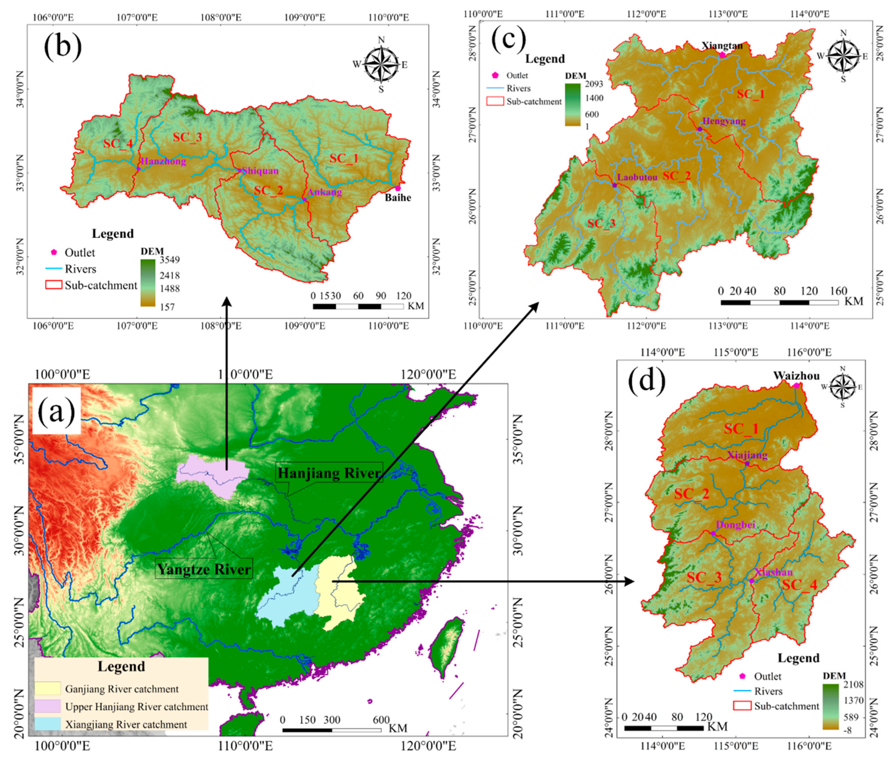
2.1. Study Area

Three experimental catchments considered in this study are the Upper Hanjiang River Catchment, the Xiangjiang River Catchment, and the Ganjiang River Catchment. They all lie in the Yangtze River basin (see Figure 1a). Since the hydrological models were run using a semi-distributed scheme, each catchment was delineated into sub-catchments. Models were calibrated against observed streamflow at the catchment outlets, i.e., Baihe, Xiangtan, and Waizhou hydrological stations. It should be mentioned that two of them, which are the Xiangjiang River Catchment and the Ganjiang River Catchment, are geographically contiguous. In that regard, these two catchments were selected for ungauged studies.

2.1.1. Upper Hanjiang River Catchment

The Hanjiang River is the longest tributary of the Yangtze River in central China. It rises in the Mountains Bozhong, flowing into the Yangtze at Wuhan, which is the provincial capital city of Hubei. The length of the Hanjiang River is about 1530 km. The Baihe hydrological station is located at the Upper Hanjiang River, as shown in Figure 1b. The catchment area above the Baihe Station is 59,115 km² (106°14′–110°27′E and 31°49′–34°38′N). This study area is classified as a semi-humid climate and mountainous region. The observed mean annual runoff and precipitation are about 370.8 mm and 876 mm, respectively. Hereafter, this catchment will be called the Hanjiang River Catchment.

2.1.2. Xiangjiang River Catchment

Xiangjiang River is another important tributary of the Yangtze River, which rises in the Guangxi province and flows into the Hunan province. With a total length of 800 km, Xiangjiang River has a river basin area of about 94,721 km². The outlet of Xiangjiang River is the Xiangtan hydrological station. The Xiangjiang River catchment located between 110°43′–114°22′E and 24°91′–28°18′N, with a total drainage area of approximately 81,638 km². The overview of the Xiangjiang River catchment is illustrated in Figure 1c. The mean annual runoff of the Xiangjiang River catchment at the Xiangtan station is about 818.9 mm. Under a subtropical monsoon climate, the mean annual precipitation ranges from 1350 to 1830 mm. The mean annual temperature is about 17.4 ℃. For more information about the Xiangjiang River catchment, we refer the reader to Zhu et al. [47].

2.1.3. Ganjiang River Basin

The Ganjiang River, which is one of the principal southern tributaries of the Yangtze River, is about 766 km in length and the major geographical backbone of Jiangxi province, China. The Ganjiang River flows north through Jiangxi province into Lake Poyang and then into the Yangtze River. The Ganjiang River basin, shown in Figure 1d, covers a drainage area of 80,948 km² above the Waizhou hydrological station (28°38′N, 115°50′E) located within 24°30′–28°42′N and 113°42′–116°38′E. The mean annual runoff of the Ganjiang River at the Waizhou station is about 845.34 mm. The Ganjiang River basin has a typical humid subtropical climate with short, cool, damp winters, and very hot, humid summers. The average annual precipitation is approximately 1506.6 mm. Much of the rainfall occurs during the late spring and summer [48].

2.2. Data Description

Potential evapotranspiration (PET), precipitation, and observed hydrological data used in this study were at a daily time step. Observed meteorological data (i.e., precipitation and temperature) were obtained from the National Climate Center of the China Meteorological Administration (Source: http://cdc.cma.gov.cn). Daily potential evapotranspiration for the analyses in this paper was calculated from daytime hours and daily temperature with the Blaney-Criddle method [49]. Catchment average precipitation was interpolated using an inverse distance weighted method (IDW). Daily streamflow data were both collected from the Bureau of Hydrology, Changjiang (Yangtze) Water Resources Commission. Ten-year streamflow data at the daily step for study catchments were used in this study (

Table 1. Information on sub-catchments, their area, and data used in the semi-distributed setup. The bold name indicates the outlet of catchment.

Sub-Catchment	Upper Hanjiang River
	Hydrological station	Area (km2)	Data period
SC_1	Baihe	20,490	2008-2017
SC_2	Ankang	14,820	--
SC_3	Shiquan	14,476	--
SC_4	Hanzhong	9329	--
Sub-Catchment	Xiangjiang River
	Hydrological station	Area (km2)	Data period
SC_1	Xiangtan	29,518	2007-2016
SC_2	Hengyang	30,779	2007-2016
SC_3	Laobutou	21,341	--
Sub-Catchment	Ganjiang River
	Hydrological station	Area (km2)	Data period
SC_1	Waizhou	18,224	2000-2009
SC_2	Xiajiang	22,493	2000-2009
SC_3	Dongbei	24,198	--
SC_4	Xiashan	16,033	--

). For a model application, the first two years of the data were used as a warm-up period, the next five years were used for calibration, and the following three years were used for independent validation.

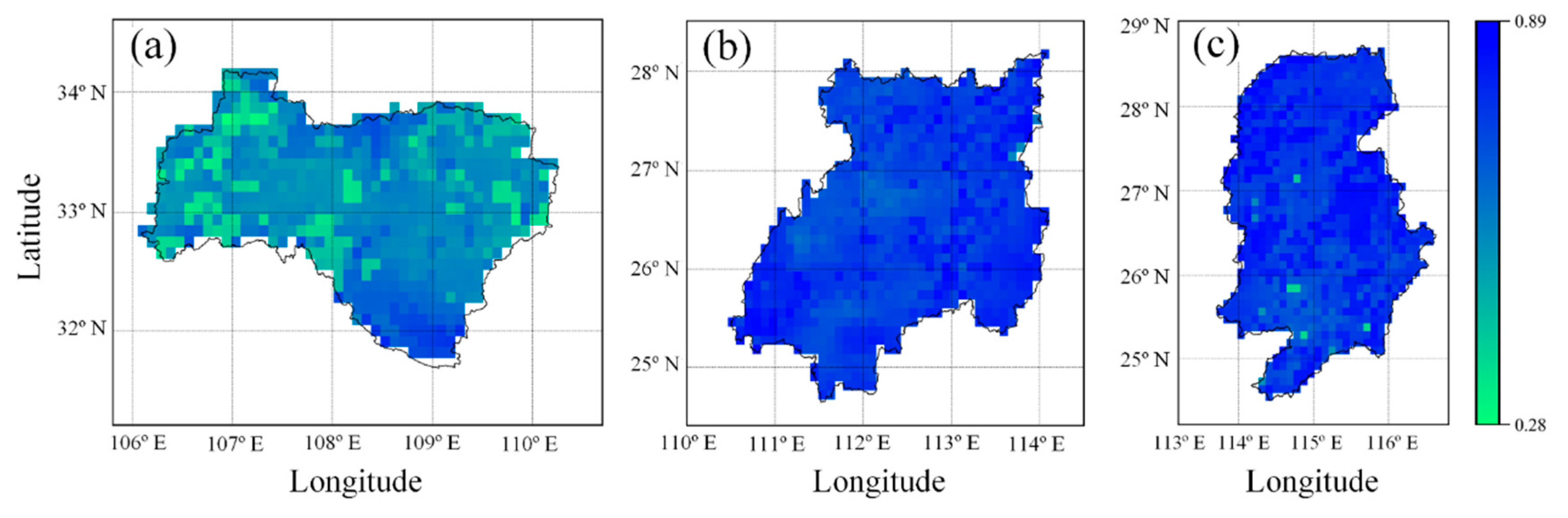
2.3. SMAP Root-Zone Soil Moisture Data

The National Aeronautics and Space Administration (NASA) has developed a Soil Moisture Active/Passive (SMAP) mission [16], which was launched in January 2015. It aims to obtain a global mapping of soil moisture by utilizing a passive L-band radiometer combined with an active L-band radar. The SMAP mission provides four levels of data products, and they are freely available at https://smap.jpl.nasa.gov/data/. The potential applications of SMAP products for hydrology research have been widely reported [50,51]. In this study, the three-hour SMAP Level 4 Surface and Root Zone Soil Moisture Geophysical Data (SPL4SMGP) [52] was selected as the source of root-zone soil moisture data due to its relatively high spatial resolution. The spatial coverage of SMAP Level 4 root-zone soil moisture data spans from 180°W to 180°E with a spatial resolution of 9 km. The root-zone soil moisture has been provided as volumetric percent or soil wetness united by SPL4SMGP. We chose the soil wetness units (dimensionless), which vary between 0 and 1. This indicates relative saturation between completely dry conditions and completely saturated conditions, respectively.

Root-zone soil moisture data were extracted over study catchments from SMAP global products from 31 March, 2015 to 28 March, 2019. Figure 2 demonstrates the map of temporal average values of SMAP root-zone soil moisture over the Hanjiang River catchment, the Xiangjiang River catchment, and the Ganjiang River catchment. The observed spatial patterns of soil moisture within the three catchments appear consistent with topography. The root-zone soil moisture varies from 0.28 to 0.79 over the Hanjiang River catchment, from 0.57 to 0.89 over the Xiangjiang River catchment, and from 0.38 to 0.89 over the Ganjiang River catchment.

3. Methodology

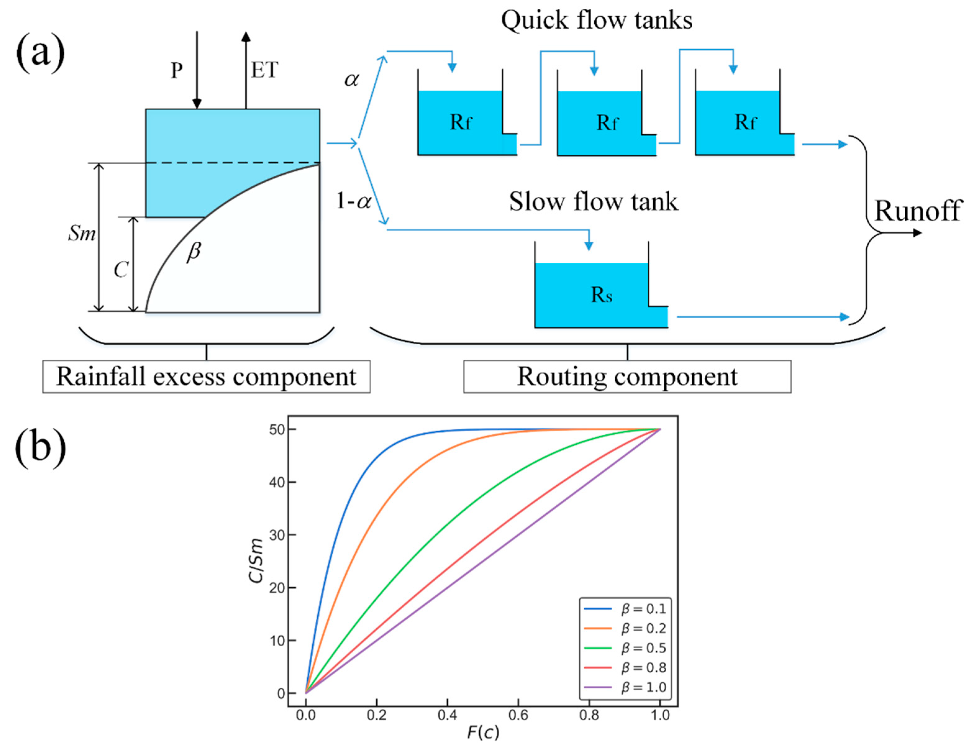
3.1. Structure of Hymod Model

A parsimonious conceptual rainfall-runoff model structure of the Hymod model was adopted in this case study. The Hymod model has been widely applied in hydrological modeling and provided satisfactory performance [53,54,55,56]. This five-parameter model is based on the probability-distribution model (PDM) proposed by Moore [57] and was originally introduced by Boyle et al. [58]. As shown in Figure 3a, the model structure consists of two main components, which are the rainfall excess component and the routing component.

Table 2. Description and prior uncertainty ranges of the Hymod model parameters.

Parameter	Model Part	Description	Unit	Prior Range
Sm	Rainfall excess	Maximum soil moisture storage capacity	mm	0–500
β	Rainfall excess	The degree of spatial variability of soil moisture storage capacity	--	0–2
α	Routing	The split parameter to divide the excess rainfall	--	0–1
Rs	Routing	The slow flow residence time of the conceptual linear reservoir	day	0–0.1
Rf	Routing	The fast flow residence time of three conceptual linear reservoirs	day	0.1–1

presents a brief description of the free parameters of the Hymod model.

The core of the Hymod model is a two-parameter nonlinear tank with a rainfall excess component. In order to split the rainfall into direct runoff and subsurface runoff, this tank statistically describes the heterogeneous spatial distribution of soil moisture storage capability. It is hypothesized that the soil moisture storage capacity $C$ varies across the catchment and has a maximum soil moisture storage capacity, $Sm$. Thus, this tank allows deriving the saturated proportion of a catchment and its relative saturation. In practice, a Pareto distribution function describes the fraction of the catchment having a storage capacity $C$.

$$F\left(C\right)=1-{\left(1-\frac{C}{Sm}\right)}^{\beta },\hspace{1em}0\le C\le Sm$$

(1)

where $C$ denotes the soil moisture storage capacity, $Sm\left[\mathrm{mm}\right]$ is the maximum soil moisture storage capacity in the catchment, and parameter $\beta [-]$ defines the degree of spatial variability of storage capacities over the catchment (see Figure 3a). Figure 3b demonstrates the examples of Equation (1), which is plotted for different values of attention $\beta$. The corresponding probability density function of the soil moisture storage capacity is shown below.

$$f\left(C\right)=\frac{dF\left(C\right)}{dC}=\frac{\beta }{Sm}{\left(1-\frac{C}{Sm}\right)}^{\beta -1},\hspace{1em}0\le C\le Sm$$

(2)

A similar function is also employed in the Xinanjiang model [59] and the Variable Infiltration Capacity (VIC) model [60]. Figure 3a illustrates that the area producing fast runoff is calculated from the proportion of the catchment with saturated reservoirs. The effective rainfall is equal to the soil moisture excess calculated at each time step.

The routing component consists of two series of linear reservoirs, a single reservoir for the slow flow, and three identical quick flow reservoirs (Figure 3a). The slow flow reservoir, modelled using one linear reservoir, represents the groundwater. The quick flow is routed by surface runoff using a cascade of three linear quick flow reservoirs. A more detailed description of the Hymod model can be found in Moore [61].

3.2. Semi-Distributed Model Setup

In this study, the Hymod model was set up using a semi-distributed modelling system. The semi-distributed scheme was applied in two catchments, which had been respectively delineated into three sub-catchments. Modelling at each sub-catchment was performed using the lumped version of the Hymod model. The river routing between sub-catchments was conducted by a linear Muskingum river model [62]. The forcing data (i.e., precipitation and potential evapotranspiration) was interpolated, according to sub-catchment boundaries with the purpose of running a semi-distributed model. Only the streamflow data at the outlet station were used for calibration. The lumped Hymod model was run at each sub-catchment, and the same set of parameters was estimated for all sub-catchments. Since the amount of sub-catchment is small and the area of each sub-catchment is similar, two parameters in the Muskingum routing model were both treated as homogeneous. As a result, in addition to the parameters of the Hymod model, the Muskingum river model has two free parameters that need to be calibrated.

3.3. Prior Estimation of the Degree of Parameter β

The prior estimation of the $\beta$ was conducted by using SMAP root-zone soil moisture data based on the method of moments. As mentioned in Section 3.1, $\beta$ is the shape parameter of Pareto distribution, which was utilized to describe the spatial variability of soil moisture storage capability. This spatial distribution can be related to different soil moisture storage capacity among the study catchment.

The form of the curve of the spatial distribution of soil moisture storage capacity is shown in Equation (2), and the first theoretical moment of Equation (2) is shown below.

$$E(C)={\displaystyle {\int }_0^{Sm}C\cdot f\left(C\right)}dC=\frac{Sm}{\beta +1}$$

(3)

Solving for $\beta$ in Equation (3) gives the following.

$$\beta =\frac{Sm}{E\left(C\right)}-1$$

(4)

In this study, SMAP root-zone soil moisture data were used to yield the samples ($S{R}_i$) for the soil moisture storage capacity $C$. For each cell of SMAP data, the soil moisture storage capacity sample $S{R}_i$ of the i-th cell could be estimated as follows:

$${\theta }_i^{\max }=\underset{1\le t\le T}{\max }{\theta }_i\left(t\right)$$

(5)

$${\theta }_i^{\min }=\underset{1\le t\le T}{\min }{\theta }_i\left(t\right)$$

(6)

$$S{R}_i=\left({\theta }_i^{\max }-{\theta }_i^{\min }\right)\cdot L$$

(7)

where ${\theta }_i\left(t\right)$ means the SMAP root-zone soil moisture for the i-th cell at the time step $t$, $T$ is the total number of time steps, and $L$ is the depth of the root zone. Note that Equation (7) is based on the assumption that the soil moisture will reach the maximum and minimum soil wetness at least once during the study period.

According to the definition, $Sm$ can be denoted by the formula below.

$$Sm=\underset{1\le i\le N}{\max }\left(S{R}_i\right)$$

(8)

where N is the total number of cells over the whole catchment or sub-catchment. Additionally, the sample mean $\overline{SR}$ could substitute the $E(C)$ in Equation (4). Hence, for Equation (4), the method of moments estimator for parameter $\beta$ can be derived from SMAP root-zone soil moisture data by using Equation (9).

$$\widehat{\beta }=\frac{\underset{1\le i\le N}{\max }\left({\theta }_i^{\max }-{\theta }_i^{\min }\right)}{\frac{1}{N}{\displaystyle {\sum }_{i=1}^N\left({\theta }_i^{\max }-{\theta }_i^{\min }\right)}}-1$$

(9)

where $\widehat{\beta }$ refers to a prior estimate of the parameter $\beta$. The estimated $\widehat{\beta }$ can be used to substitute the free parameter $\beta$ before calibration.

3.4. Model Calibration Methodology and Performance Evaluation

Estimation of posterior distributions of free model parameters was performed using the Differential Evolution Adaptive Metropolis (DREAM) algorithm developed by Vrugt et al. [63]. The DREAM has been widely and successfully used in hydrological research and applications [64,65,66]. This method uses the Bayesian framework where model parameters are treated as probabilistic variables. The prior parameter distribution $P\left(\theta |x\right)$ is utilized to infer posterior parameter distribution $P\left(\theta |Q,x\right)$ by using Equation (10).

$$P\left(\theta |Q,x\right)\propto L\left(Q|\theta ,x\right)P\left(\theta |x\right)$$

(10)

where $L\left(Q|\theta ,x\right)$ represents a likelihood function. DREAM infers the posterior probability distribution of calibrated model parameter values with an adaptive Markov Chain Monte Carlo (MCMC) sampling. In this study, we used the sum of absolute error residuals as a likelihood function [67]. The prior distribution of free parameters of the Hymod model was assumed to be uniform (noninformative) prior distributions and the ranges of each parameter are listed in Table 2. DREAM runs multiple chains simultaneously, which walk through the parameter space for global exploration. A Gelman and Rubin [68] criterion was used for monitoring whether each chain converges to a stationary distribution. The final posterior distributions are generated from 8000 samples and, additionally, an ensemble of 2000 parameter sets was obtained in this study, which represents the final posterior probability distribution.

In order to evaluate the streamflow modelling results at the catchment outlet, two performance criteria were used to assess the objective model efficiency in the calibration and validation periods, including Nash-Sutcliffe Efficiency (NSE) [69] and Kling-Gupta efficiency (KGE) [70].

NSE values emphasizes the high flow when it is utilized to evaluate the predictive skill. The score of 1 indicates that the simulated discharges perfectly match the observations. A negative value implies that the simulated discharges are worse than using the average value of the observations. NSE is defined by the equation below.

$$\mathrm{NSE}=1-\frac{{\displaystyle {\sum }_{j=1}^n{\left(Q_{sim,j}-Q_{obs,j}\right)}^2}}{{\displaystyle {\sum }_{j=1}^n{\left(Q_{obs,j}-\overline{Q_{obs,j}}\right)}^2}}$$

(11)

where $Q_{sim,j}$ and $Q_{obs,j}$ are the simulated and observed values of streamflow at the j-th step and n is the total number of time steps.

KGE optimizes for the bias, variability, and correlation simultaneously, and it is sensitive to both high flow and variance. KGE is defined as Equation (12) below.

$$\mathrm{KGE}=1-\sqrt{\left(r-1\right)+\left(a-1\right)+\left(b-1\right)}$$

(12)

where $r$ is the Pearson correlation coefficient between the simulations and observations, $a$ is the ratio between the variance of the simulations and the variance of the observations, and $b$ is the ratio of the means of the simulations and observations. KGE ranges from $-\infty$ to 1 with an ideal value of 1.

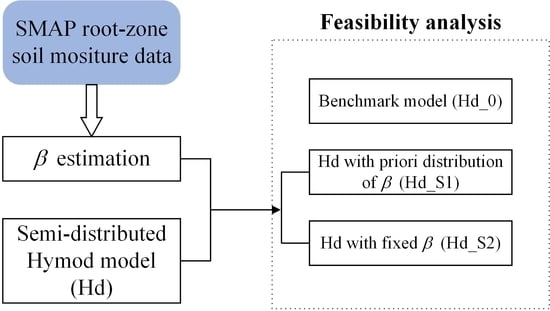
3.5. Experimental Design

An original model setup and two experimental scenarios were established to assess the impact of incorporating the SMAP root-zone soil moisture data. These three model setups were calibrated against daily streamflow at outlets of three study catchments. The original semi-distributed Hymod model (Hd_0) served as a benchmark. Details of two experimental model setups are described as follows.

(1) Scenario one (Hd_S1): In the first experimental scenario, the semi-distributed setup of the Hymod model included an informative priori distribution of $\beta$. To derive the priori distribution of $\beta$, a moving window with a length of 15 months was applied to the whole period (about 48 months). For each window, a $\beta$ could be calculated for the whole catchment using the method mentioned in Section 3.2. A total of 34 samples could be obtained for each study catchment. These samples fitted a uniform distribution between the defined range from the minimum of samples to the maximum of samples, which would, consequently, be used as priori distribution for the $\beta$.

(2) Scenario two (Hd_S2): In this scenario, the parameter $\beta$ was fixed at each sub-catchment using SMAP data for the whole period rather than being calibrated. As a result, this scenario has six free parameters to calibrate.

Additionally, in order to evaluate the robustness of Hd_S2 using the estimated $\beta$, the Xiangjiang River Catchment and the Ganjiang River Catchment would be assumed as “ungauged” catchments.

4. Results and Discussion

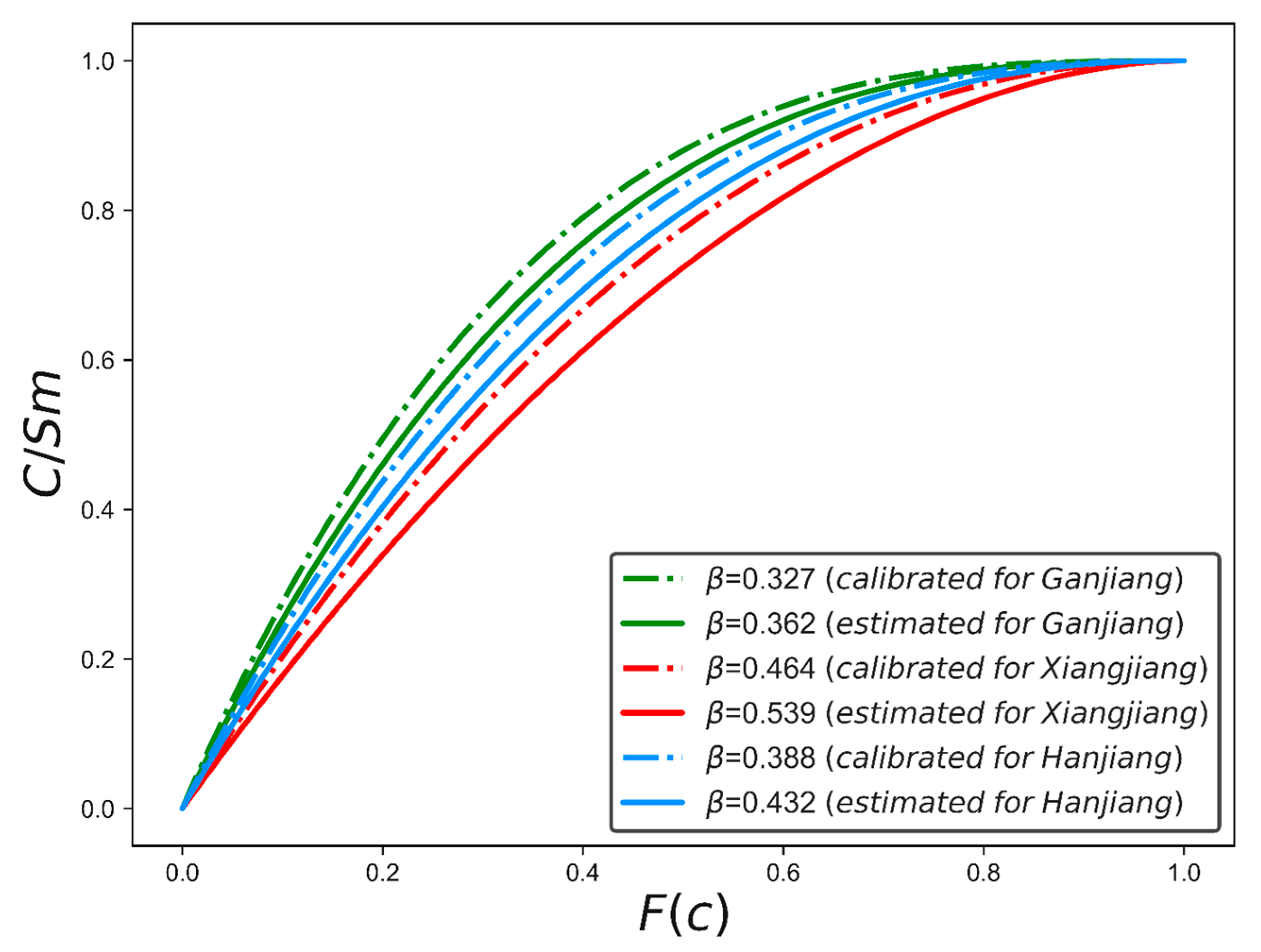
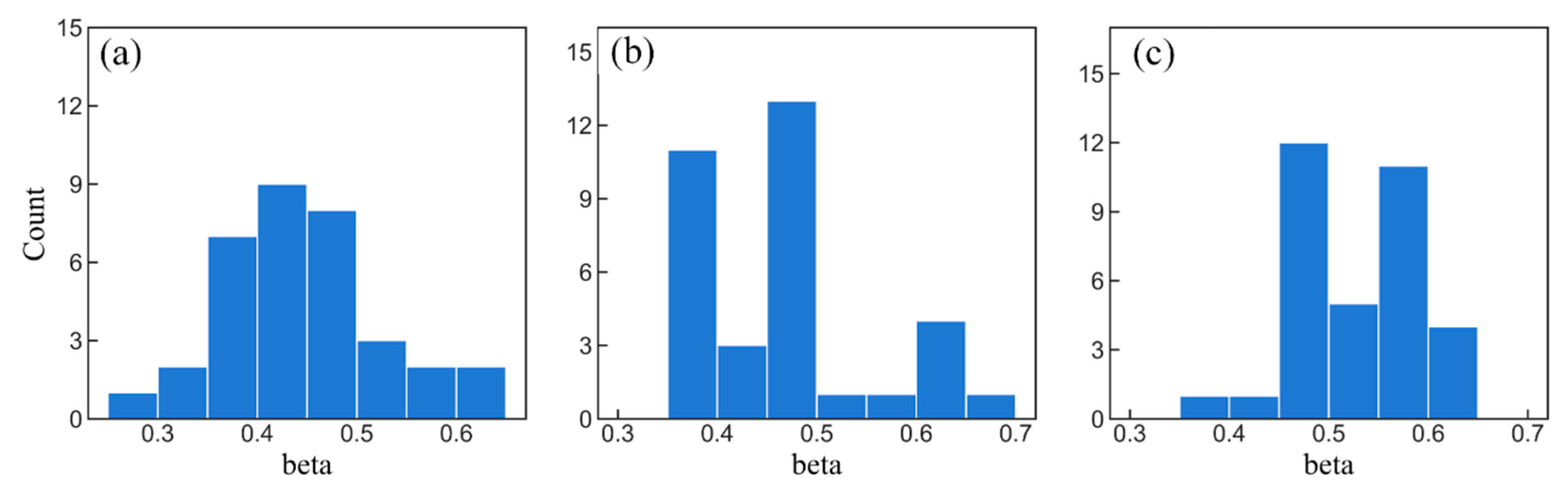
4.1. Results of the Estimated β Value and Its Uncertainty

The parameter $\beta$ controls the spatial heterogeneity of soil moisture storage capacity, and it has been commonly calibrated against observed streamflow. We plotted the distributions of soil moisture storage capacity for different $\beta$ values based on the estimation method described in Section 3.3 and the model calibration method. Figure 4 compares the distributions of soil moisture storage capacity of three study catchments. The values of $\beta$ vary at different catchments since the parameter $\beta$ is affected by factors like topography, land cover, and soil texture. Considering the same catchment, two methods produced comparable $\beta$ values. They showed low differences (0.044 for the Hanjiang River Catchment, 0.075 for the Xiangjiang River Catchment, and 0.035 for the Ganjiang River Catchment), which suggests that the prior estimation method proposed in Section 3.3 is reliable.

Choosing different periods of SMAP root-zone soil moisture data could lead to different $\beta$ samples. Figure 5 shows the sampled values for the parameter $\beta$ at each catchment using the sampling strategy mentioned in Section 3.5. Compared to the original range of parameter $\beta$, narrower ranges were produced for parameter $\beta$ at each catchment, which were [0.258, 0.644] for the Hanjiang River Catchment, [0.363, 0.689] for the Xiangjiang River Catchment, and [0.375, 0.607] for the Ganjiang River Catchment. These values were utilized as a prior range for the parameter $\beta$ in Hd_S1, while original Hd_0 still simply employed a uniform distribution of the range [0, 2]. Since the $\beta$ value represents the spatial variability of soil moisture storage capacity, their uncertainties derived from SMAP root-zone soil moisture data were found to be relatively low. The results suggested that the spatial patterns of soil moisture storage capacity are stable.

We only considered the difference of periods as the source of uncertainty for the $\beta$ parameter in this study. To estimate the value of $\beta$ using the method described in Section 3.3, the spatial resolution of soil moisture data is also important, due to the fact that coarse spatial resolution can hardly represent the spatial variability of soil moisture capacity at the same spatial scale. As a result, it would generate more uncertainty on parameter $\beta$. Therefore, further investigations should be carried out concerning the spatial resolution of soil moisture data.

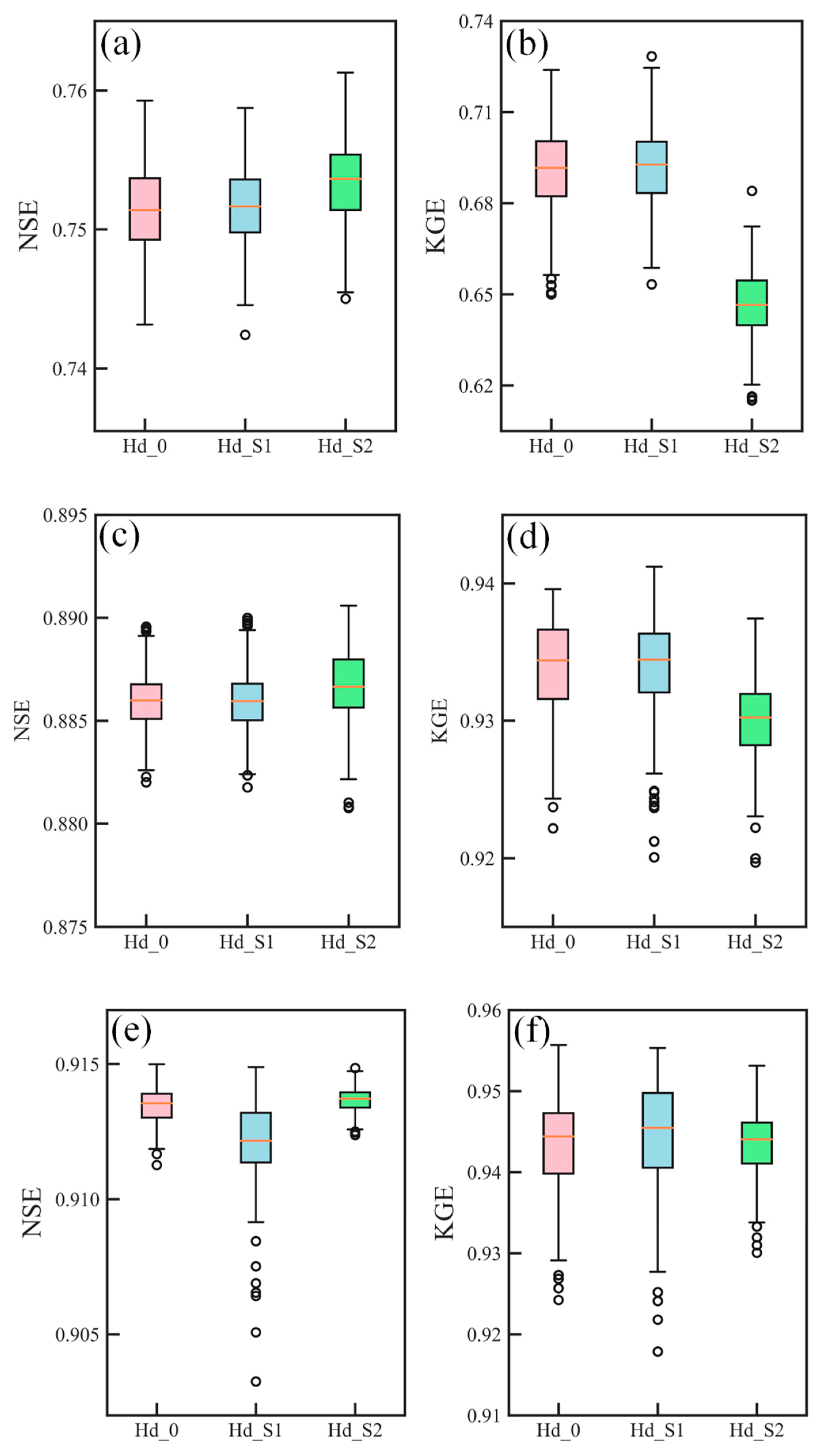
4.2. Comparison of Model Simulations

For further evaluation of the feasibility of estimated $\beta$ values, the performances of three model setups (see Section 3.5) were compared in this section. Three model setups were calibrated to daily streamflow observations at catchment outlets, i.e., the Baihe station, the Xiangtan station, and the Waizhou station. All 2000 calibrated parameter sets obtained from the DREAM method (see Section 3.4) were then used to perform a prediction in validation periods. Two statistics, i.e., NSE and KGE, were applied to evaluate the model efficiency for the calibration and validation periods.

Table 3. Model performance, in terms of NSE and KGE, for the calibration period. The bold values indicate the best performance.

Model Setup	Baihe Station (Hanjiang River)		Xiangtan Station (Xiangjiang River)		Waizhou Station (Ganjiang River)
	NSE (%)	KGE (%)	NSE (%)	KGE (%)	NSE (%)	KGE (%)
Hd_0	82.70	81.15	89.26	93.38	92.33	95.37
Hd_S1	82.70	81.35	89.26	93.45	92.31	95.73
Hd_S2	82.46	80.19	89.24	92.90	92.31	95.28

and

Table 4. Model performance, in terms of NSE and KGE, for the calibration period. The bold values indicate the best performance.

Model Setup	Baihe Station (Hanjiang River)		Xiangtan Station (Xiangjiang River)		Waizhou Station (Ganjiang River)
	NSE (%)	KGE (%)	NSE (%)	KGE (%)	NSE (%)	KGE (%)
Hd_0	75.93	72.39	88.96	93.96	91.50	95.57
Hd_S1	75.87	72.84	89.00	94.12	91.49	95.53
Hd_S2	76.13	68.41	89.06	93.74	91.49	95.31

display the best NSE/KGE results for the three catchments during calibration and validation periods, respectively, for the three catchments. Note that larger NSE and KGE values indicate a better model performance.

For the calibration period, the individual results across three catchments reached high scores (Table 3), which indicates that the semi-distributed Hymod model is suitable for selected study catchments. It was found that the Hd_0 and Hd_S1 produce comparable results. The Hd_0 always provided the highest NSE values, while the Hd_S1 produced the highest KGE. The Hd_S2 resulted in slightly lower NSE and KGE values due to the smaller number of free parameters. However, it is encouraging to find that differences in NSE/KGE between the Hd_S2 and Hd_0 were 0.24%/0.96% for the Hanjiang River catchment, 0.02%/0.48% for the Xiangjiang River catchment, and 0.02%/0.09% for the Ganjiang River catchment. The slight differences infer that using uncalibrated $\beta$ values did not sharply deteriorate model efficiency.

For the validation period (see Table 4), the results demonstrated that Hd_0 only showed the best performance at the Ganjiang River catchment. For the Hanjiang River catchments and the Xiangjiang River catchments, Hd_S2 resulted in best model performance in terms of NSE (76.13% for the Hanjiang River catchment and 89.06% for the Xiangjiang River catchment), and Hd_S1 showed the best KGE values (72.84% for the Hanjiang River catchment and 94.12% for the Xiangjiang River catchment). Hd_0 showed worse predictions when compared with both the Hd_S1 and Hd_S2. This can be explained by the equifinality issue in hydrological modelling. Both Hd_S1 and Hd_S2 showed better consistency compared to the Hd_0.

In order to consider the prediction uncertainty of the model setups, boxplots of the NSE and KGE values concerning all 2000 calibrated parameter sets were given in Figure 6. Figure 6 demonstrates a more comprehensive comparison of simulation performances during validation periods, which compared the distribution of the three metrics obtained from Hd_0, Hd_S1, and Hd_S2 at the validation period. For NSE values, Hd_S2 always provided better values. Considering KGE values, Hd_S1 could give a better performance. The explanation for this can be that constraining the value of the $\beta$ parameter could reduce equifinality.

In summary, the results showed that Hd_S1 and Hd_S2 using the prior estimation of the $\beta$ were able to produce consistent streamflow predictions in study catchments in terms of NSE/KGE. The results indicated that the estimated $\beta$ values were feasible in the semi-distributed Hymod model.

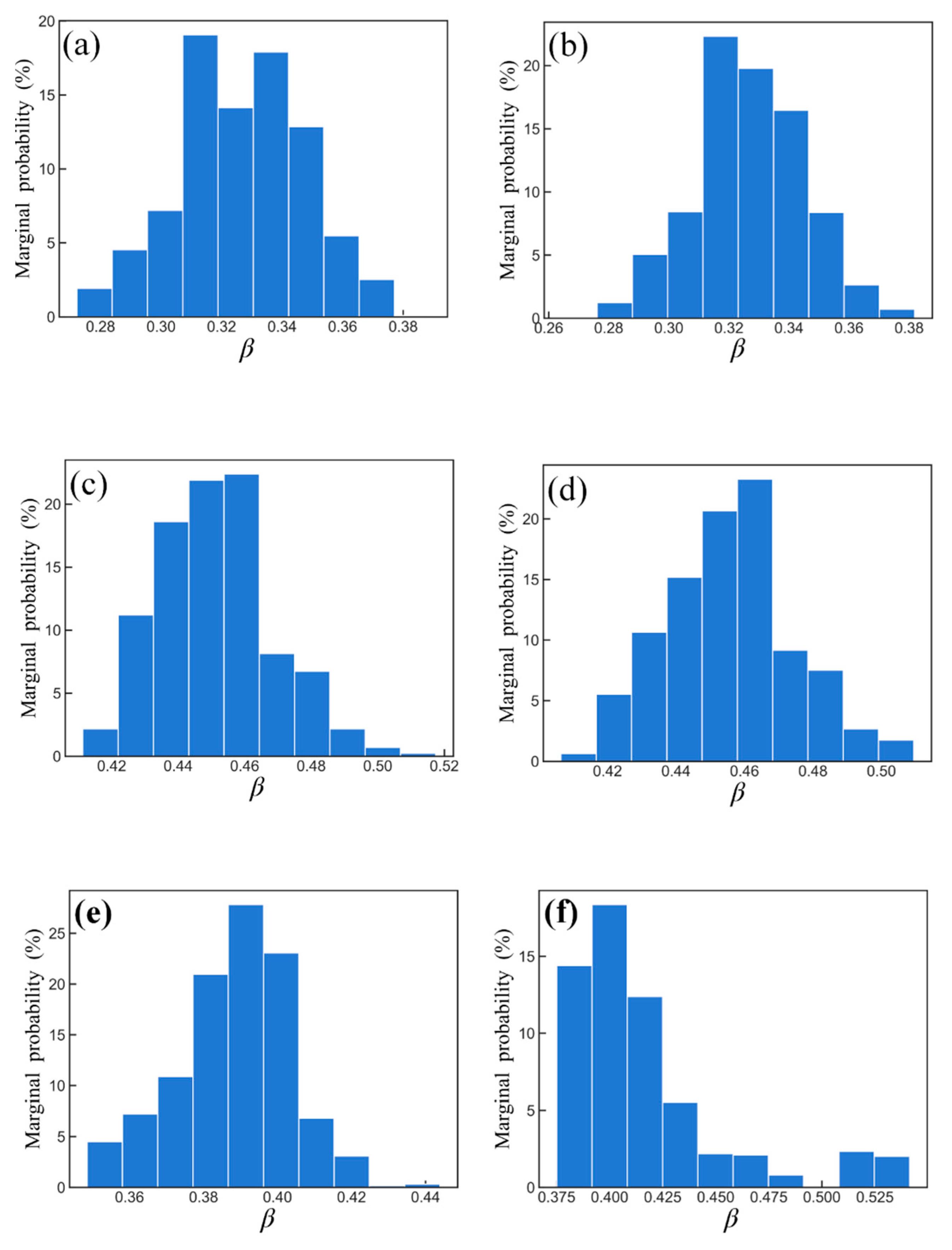
4.3. Analysis of the Posterior Distribution of β

As mentioned in Section 3.4, the DREAM algorithm was employed to estimate model parameter posterior distribution. In this scenario, we analyzed the parameter uncertainty based on the final 2000 samples after convergence. Figure 7 shows the marginal posterior distribution of the $\beta$ parameter. The comparison between the priori distribution of $\beta$ (Figure 4) and the posterior distribution derived from Hd_S1 (left panels of Figure 7) could suggest whether samples of $\beta$ are able to supply reliable prior information for Hd_S1. As shown in Figure 7, the prior ranges of $\beta$ provided by SMAP soil moisture data could cover the posterior ranges.

The distance between two posterior distributions of parameter $\beta$ derived from Hd_0 and Hd_S1 were determined to assess the reliability of information added to the model. With the probability values of 0.32 (Hd_0) and 0.31 (Hd_S1) for the Hanjiang River Catchment, 0.46 (Hd_0) and 0.46 (Hd_S1) for the Xiangjiang River Catchment, and 0.39 (Hd_0) and 0.40 (Hd_S1) for the Ganjiang River Catchment, we found that the $\beta$ parameter for all six setups was well-identified.

The derived posterior distributions for $\beta$ all showed an approximately normal distribution. For the same catchment, values of $\beta$ from Hd_0 and Hd_S1 are located at almost the same points. Since the prior distribution of $\beta$ was constrained in Hd_S1 by information extracted by SMAP soil moisture data, it could be inferred that the boundaries are reliable. By comparing posterior distributions of $\beta$, it can be concluded that the uncertainties generated from different periods are reasonable. The similar posterior distributions also indicated that the method for an estimate of $\beta$ was feasible.

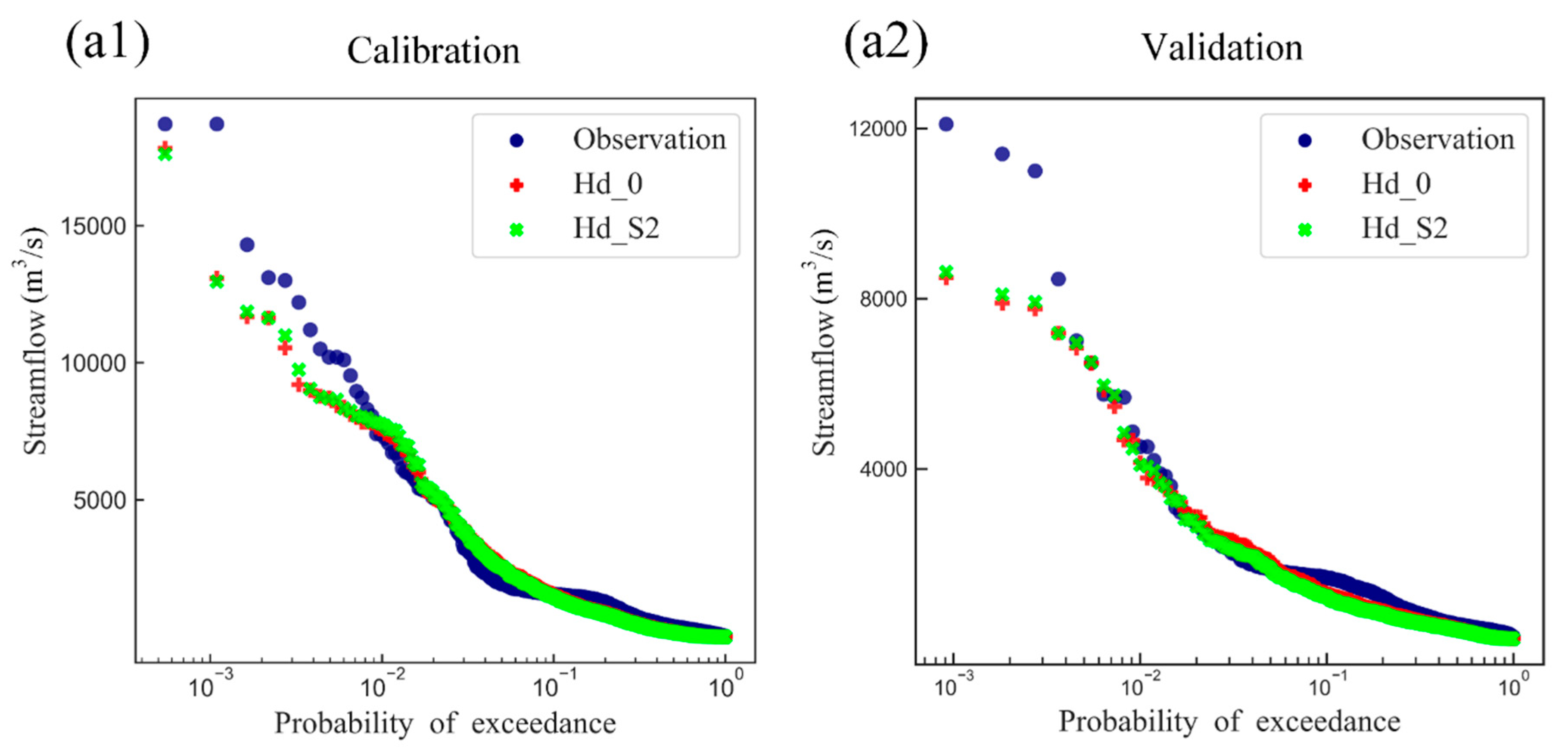
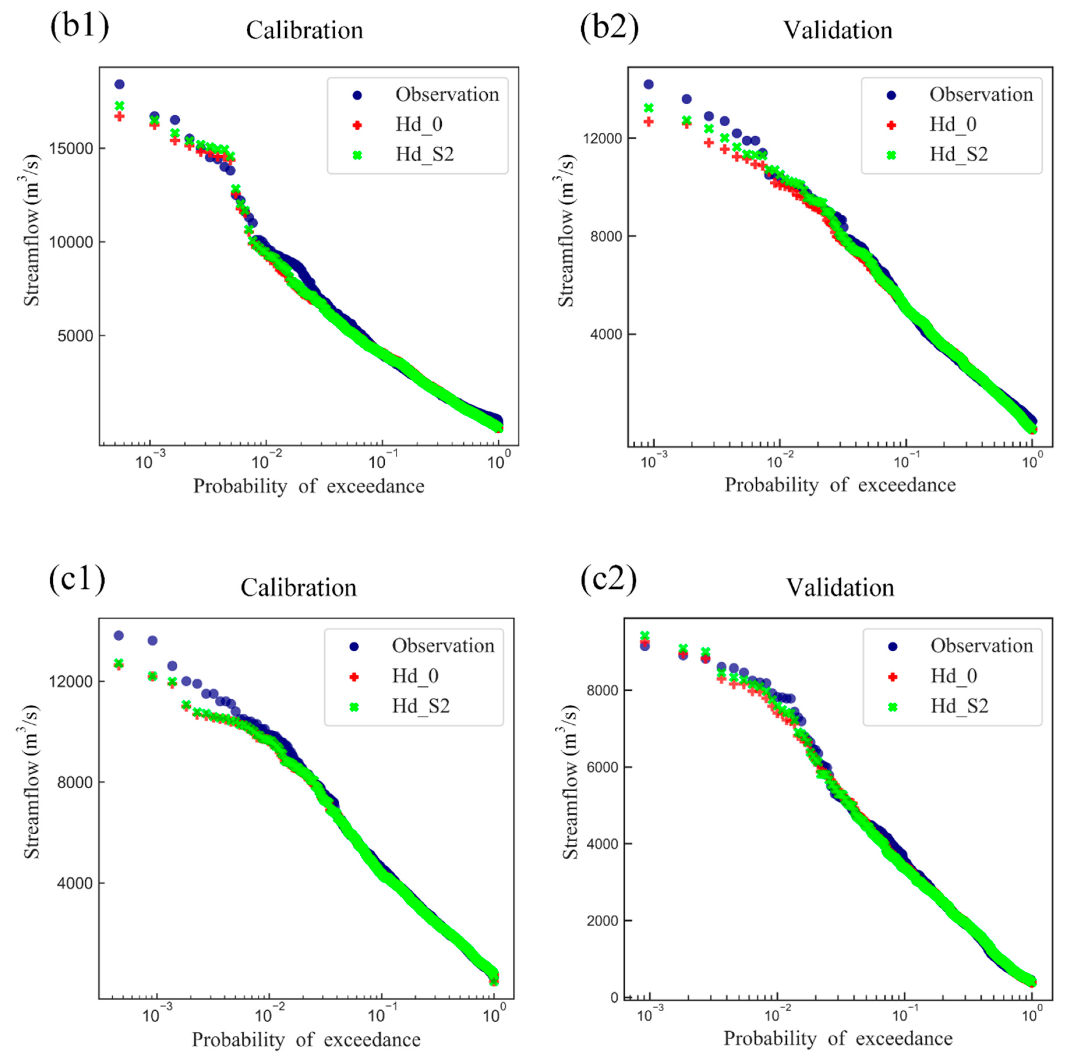
4.4. Streamflow Signature (Flow Duration Curves)

Flow Duration Curves (FDC) are derived from the simulated and observed streamflow data. FDC represents the probability of a given flow being exceeded or equaled. It is one of the typical hydrological signatures to evaluate the model behavior of a catchment, which provides insights about how streamflow is distributed across high to low flow regimes [71].

In Figure 8b,c, the Xiangjiang River catchments and the Ganjiang River catchments show an approximate linear FDC, while the Hanjiang River catchment shows a nonlinear curve (Figure 8a). The nonlinear curve in the Hanjiang River Catchment indicates that observed data at calibration and validation periods constitute a disproportional representation of high, medium, and low flow regimes [66]. The nonlinearity in the Hanjiang River catchment may lead to lower simulation performance than the Xiangjiang River catchment. The results of the comparison between Hd_0 and Hd_S2 simulations and observations show that the low flows in both the Hanjiang River catchments and the Xiangjiang River catchments were well captured during calibration and validation periods.

For all three catchments, Hd_0 and Hd_S2 provided comparable FDC in the calibration period while the benchmark setup (i.e., Hd_0) underestimates high flows at validation. This could explain the results that the NSE value of Hd_S2 is higher than the Benchmark setup in the validation period (seeTable 4).

In summary, the prior estimation of parameter $\beta$ leads to a consistent improvement of streamflow simulations during the validation period since the ability of the simulated high flows were improved.

4.5. Impact on Prediction Ability at Ungauged Locations

To assess the reliability of the estimated $\beta$, a comparison was conducted at ungauged catchments. As shown in Section 3.5, only the Xiangjiang River catchment and the Ganjiang River catchment were selected for an ungauged catchment study, because they are geographically contiguous. Each of them were treated as “ungauged” when the other acted as a donor catchment. At ungauged catchment, the streamflow data was considered unavailable, but model input, i.e., precipitation and potential evapotranspiration, and SMAP soil moisture data were available. We used the proximity-based parameter transfer to evaluate predictive performance. More specifically, for the Hd_0 and Hd_S1, all parameters calibrated at donor catchment were transferred to the receiver, while, for Hd_S2, all parameters except $\beta$ were transferred to the receiver and $\beta$ was estimated using SMAP data over the receiver.

Figure 9 and Figure 10 illustrated the predictive performance during the validation period using parameter sets transferred from the donor catchment. The results showed that the prediction from Hd_S2 consistently outperformed Hd_0 and Hd_S1 in terms of NSE/KGE. Notably, the improvements at catchments including more sub-catchments (Xiangtan station and Waizhou station) were more remarkable than those with fewer sub-catchments (Hengyang station and Xiajiang station). Considering the best value of NSE/KGE, Hd_S1 and Hd_S2 showed better performance than Hd_0. According to the tests, it can be concluded that incorporating soil moisture data made the model more robust.

Using the distribution of NSE/KGE, we investigated the prediction uncertainties for ungauged catchments. Although predictions from Hd_S1 and Hd_S2 were both improved for the Xiangjiang River catchment, only the latter had reduced the uncertainties. This result could be explained by the $\beta$ value being fixed in Hd_S2, which leads to less freedom. However, it can be found that the uncertainty results at the Ganjiang River catchment were not as sensible as the Xiangjiang River catchment.

It is encouraging to find that using $\beta$ based on SMAP soil moisture data outperformed versus transferring the parameters, including $\beta$ from the donor catchment. Prediction at ungauged catchments is still challenging in hydrological modelling. The strategy for estimating parameters only using SMAP soil moisture data provide an alternative way for parameter identification at ungauged catchment.

4.6. Discussion

This study has explored the impact of using SMAP root-zone soil moisture data on estimating the parameter value of $\beta$ in the semi-distributed Hymod model. Compared to the methods of data assimilation and model calibration, the method for utilizing the soil moisture data to estimate parameters proves two benefits. For example, this method simplifies the parameter optimization procedure. Traditionally, a hydrological model is calibrated against measured streamflow data. The proposed estimation method of the parameter $\beta$ is independent of precipitation and streamflow data that are essential for data assimilation and model calibration methods [28,35]. Recent studies have suggested that adopting additional information in selecting parameter values can improve the performance of hydrological models [4,72]. It is a physically-based way of finding a suitable value for the parameter $\beta$ by only using SMAP root-zone soil data. This also explains why the semi-distributed Hymod model that uses $\beta$ has good performances at ungauged basins.

Additionally, choosing different periods of SMAP root-zone soil moisture data leads to similar results of $\beta$ value, which has been shown in Section 4.1. In the estimation procedure, the main information extracted from SMAP root-zone soil moisture data is the spatial variability, and the spatial patterns of soil moisture have been proven to be stable over time [41]. It indicated that the $\beta$ value estimated from historical SMAP data can be used to model the prediction, which means that the need for real-time data was reduced. As a result, this method can provide a lasting improvement to the model performance that should persist even when the SMAP soil moisture data become unavailable.

Note that this strategy uses SMAP data for finding suitable parameters for the hydrological model, which was only tested at three large catchments. The applicability of this estimation method might be limited at smaller catchment scales. Clearly, these estimated results $\beta$ may suffer high uncertainty at a small catchment scale, because the number of cells would be small. Currently, the spatial resolution of SMAP root-zone soil moisture data (9 km) used in this study is relatively high among the available soil moisture products. The feasibility should be analyzed at the small catchments when the root-zone soil moisture data with higher spatial resolution data are available.

The study on streamflow forecast, especially at ungauged catchment, is still the main challenge faced by the hydrological community [73,74]. The traditional process of model calibration needs abundant hydro-meteorological measurements. Along with developing earth observation techniques, the satellite-based data have shown its underlying strength for hydrological modelling [75]. Future works should focus on developing a hybrid modelling system, and coupling the physical process models with the earth observation data by expert techniques like machine learning [40]. Thus, hydrological models can potentially provide more accurate streamflow predictions by integrating more knowledge obtained from observations.

5. Conclusions

This paper introduced a prior estimation method for parameter $\beta$ in the semi-distributed Hymod model using only SMAP root-zone soil moisture data. The major objective of this study was to examine the feasibility of the estimated $\beta$ values. The examination of transferability of estimated $\beta$ alongside other calibrated parameters in time and space was conducted by the temporal and spatial transfer process. The main conclusions are as follows.

• The different results between calibrated β and estimated β values (0.044 for the Hanjiang River catchment, 0.075 for the Xiangjiang River catchment, and 0.035 for the Ganjiang River catchment) indicated that the method proposed in this study can derive reasonable β values for the Hymod model only based on SMAP soil moisture data before calibration.
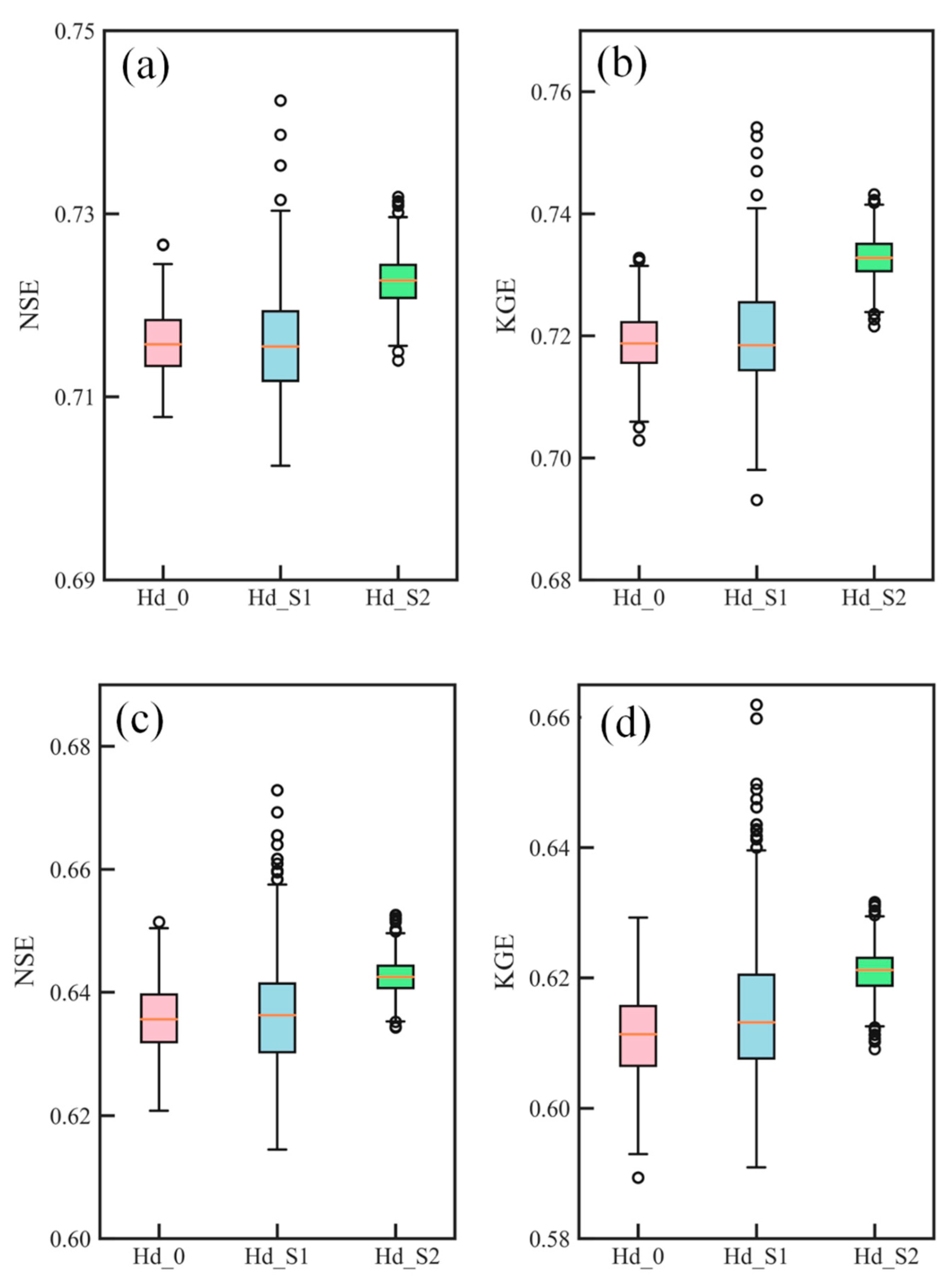
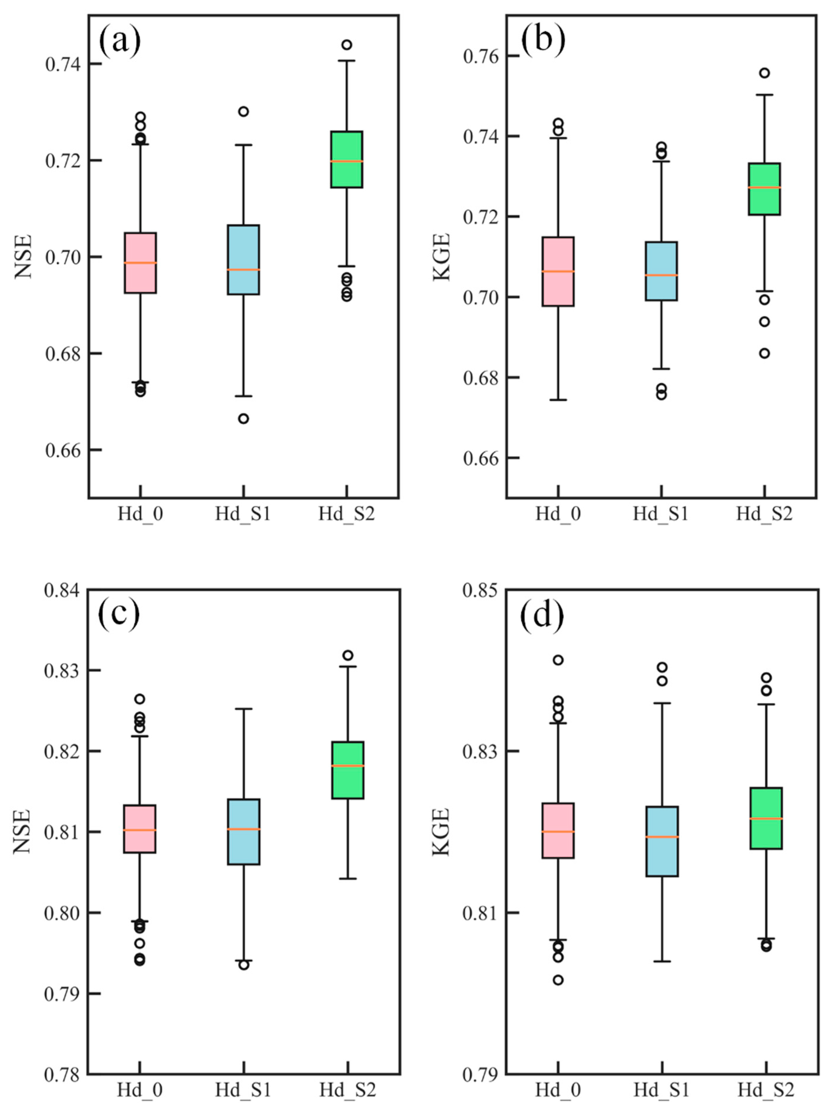
• It was found that both Hd_S1 and Hd_S2 setups both performed well in terms of NSE and KGE that are comparable to the benchmark setup (i.e. Hd_0) in the calibration period. This result indicated that the method proposed can derive a set of feasible values for the β parameter. In the validation period, the transferability of the parameter over time was tested, and a slight improvement was found. This improvement could be explained by the prior estimation of parameter β preventing over-fitting.
• More consistent improvement was generally identified at ungauged neighborhood catchments, with improved NSE values at all four stations. It was demonstrated that the information provided by root-zone soil moisture data was reasonable and increased the robustness of the model. Thus, we highlighted the value of SMAP soil moisture data for finding suitable model parameter sets for the ungauged catchment.

The results of this study emphasized the potential value of using satellite-based soil moisture data. The added information offered by the data helps us investigate hydrological processes across a wide range of spatial and temporal scales, especially for catchments with sparse hydrological data.

References

1. Rakovec, O.; Kumar, R.; Attinger, S.; Samaniego, L. Improving the realism of hydrologic model functioning through multivariate parameter estimation. Water Resour. Res. 2016, 52, 7779–7792. [Google Scholar] [CrossRef]
2. Liu, Y.; Weerts, A.; Clark, M.; Hendricks Franssen, H.-J.; Kumar, S.; Moradkhani, H.; Seo, D.-J.; Schwanenberg, D.; Smith, P.; Van Dijk, A. Advancing data assimilation in operational hydrologic forecasting: Progresses, challenges, and emerging opportunities. Hydrol. Earth Syst. Sci. 2012, 16, 3863–3887. [Google Scholar] [CrossRef]
3. Yang, H.; Xiong, L.; Ma, Q.; Xia, J.; Chen, J.; Xu, C.-Y. Utilizing satellite surface soil moisture data in calibrating a distributed hydrological model applied in humid regions through a multi-objective Bayesian hierarchical framework. Remote Sens. 2019, 11, 1335. [Google Scholar] [CrossRef]
4. Nijzink, R.C.; Almeida, S.; Pechlivanidis, I.G.; Capell, R.; Gustafssons, D.; Arheimer, B.; Parajka, J.; Freer, J.; Han, D.; Wagener, T.; et al. Constraining conceptual hydrological models with multiple information sources. Water Resour. Res. 2018, 54, 8332–8362. [Google Scholar] [CrossRef]
5. Brocca, L.; Ciabatta, L.; Massari, C.; Camici, S.; Tarpanelli, A. Soil moisture for hydrological applications: Open questions and new opportunities. Water 2017, 9, 140. [Google Scholar] [CrossRef]
6. Srivastava, P.K. Satellite soil moisture: Review of theory and applications in water resources. Water Resour. Manag. 2017, 31, 3161–3176. [Google Scholar] [CrossRef]
7. Western, A.W.; Grayson, R.B.; Blöschl, G. Scaling of soil moisture: A hydrologic perspective. Annu. Rev. Earth Planetary. Sci. 2002, 30, 149–180. [Google Scholar] [CrossRef]
8. Uber, M.; Vandervaere, J.P.; Zin, I.; Braud, I.; Heisterman, M.; Legout, C.; Molinié, G.; Nord, G. How does initial soil moisture influence the hydrological response? A case study from southern France. Hydrol. Earth Syst. Sci. 2018, 22, 6127–6146. [Google Scholar] [CrossRef] [Green Version]
9. Vereecken, H.; Schnepf, A.; Hopmans, J.W.; Javaux, M.; Or, D.; Roose, T.; Vanderborght, J.; Young, M.H.; Amelung, W.; Aitkenhead, M.; et al. Modeling soil processes: Review, key challenges, and new perspectives. Vadose Zone J. 2016, 15, 1–57. [Google Scholar] [CrossRef]
10. Wright, A.J.; Walker, J.P.; Pauwels, V.R.N. Identification of hydrologic models, optimized parameters, and rainfall inputs consistent with in situ streamflow and rainfall and remotely sensed soil moisture. J. Hydrometeorol. 2018, 19, 1305–1320. [Google Scholar] [CrossRef]
11. Mohanty, B.P.; Cosh, M.H.; Lakshmi, V.; Montzka, C. Soil moisture remote sensing: State-of-the-science. Vadose Zone J. 2017, 16. [Google Scholar] [CrossRef]
12. Babaeian, E.; Sadeghi, M.; Jones, S.B.; Montzka, C.; Vereecken, H.; Tuller, M. Ground, proximal, and satellite remote sensing of soil moisture. Rev. Geophys. 2019, 57, 530–616. [Google Scholar] [CrossRef]
13. Owe, M.; de Jeu, R.; Holmes, T. Multisensor historical climatology of satellite-derived global land surface moisture. J. Geophys. Res. Earth Surf. 2008, 113, F01002. [Google Scholar] [CrossRef]
14. Bartalis, Z.; Wagner, W.; Naeimi, V.; Hasenauer, S.; Scipal, K.; Bonekamp, H.; Figa, J.; Anderson, C. Initial soil moisture retrievals from the METOP-A Advanced Scatterometer (ASCAT). Geophys. Res. Lett. 2007, 34, L20401. [Google Scholar] [CrossRef]
15. Kerr, Y.H.; Waldteufel, P.; Wigneron, J.-P.; Delwart, S.; Cabot, F.; Boutin, J.; Escorihuela, M.-J.; Font, J.; Reul, N.; Gruhier, C. The SMOS mission: New tool for monitoring key elements of the global water cycle. Proc. IEEE 2010, 98, 666–687. [Google Scholar] [CrossRef]
16. Entekhabi, D.; Njoku, E.G.; O’Neill, P.E.; Kellogg, K.H.; Crow, W.T.; Edelstein, W.N.; Entin, J.K.; Goodman, S.D.; Jackson, T.J.; Johnson, J. The soil moisture active passive (SMAP) mission. Proc. IEEE 2010, 98, 704–716. [Google Scholar] [CrossRef]
17. Torres, R.; Snoeij, P.; Geudtner, D.; Bibby, D.; Davidson, M.; Attema, E.; Potin, P.; Rommen, B.; Floury, N.; Brown, M. GMES Sentinel-1 mission. Remote Sens. Environ. 2012, 120, 9–24. [Google Scholar] [CrossRef]
18. Peng, J.; Loew, A.; Merlin, O.; Verhoest, N.E. A review of spatial downscaling of satellite remotely sensed soil moisture. Rev. Geophys. 2017, 55, 341–366. [Google Scholar] [CrossRef]
19. Bauer-Marschallinger, B.; Freeman, V.; Cao, S.; Paulik, C.; Schaufler, S.; Stachl, T.; Modanesi, S.; Massari, C.; Ciabatta, L.; Brocca, L.; et al. Toward global soil moisture monitoring with sentinel-1: Harnessing assets and overcoming obstacles. IEEE Trans. Geosci. Remote Sens. 2019, 57, 520–539. [Google Scholar] [CrossRef]
20. Das, N.N.; Entekhabi, D.; Dunbar, R.S.; Colliander, A.; Chen, F.; Crow, W.; Jackson, T.J.; Berg, A.; Bosch, D.D.; Caldwell, T. The SMAP mission combined active-passive soil moisture product at 9 km and 3 km spatial resolutions. Remote Sens. Environ. 2018, 211, 204–217. [Google Scholar] [CrossRef]
21. Montzka, C.; Jagdhuber, T.; Horn, R.; Bogena, H.R.; Hajnsek, I.; Reigber, A.; Vereecken, H. Investigation of SMAP fusion algorithms with airborne active and passive L-band microwave remote sensing. IEEE Trans. Geosci. Remote Sens. 2016, 54, 3878–3889. [Google Scholar] [CrossRef]
22. Das, N.N.; Entekhabi, D.; Njoku, E.G.; Shi, J.J.C.; Johnson, J.T.; Colliander, A. Tests of the SMAP combined radar and radiometer algorithm using airborne field campaign observations and simulated data. IEEE Trans. Geosci. Remote Sens. 2014, 52, 2018–2028. [Google Scholar] [CrossRef]
23. Song, C.; Jia, L.; Menenti, M. Retrieving high-resolution surface soil moisture by downscaling AMSR-E brightness temperature using MODIS LST and NDVI data. IEEE J. Sel. Top. Appl. Earth Obs. Remote Sens. 2014, 7, 935–942. [Google Scholar] [CrossRef]
24. Srivastava, P.K.; Han, D.; Ramirez, M.R.; Islam, T. Machine learning techniques for downscaling SMOS satellite soil moisture using MODIS land surface temperature for hydrological application. Water Resour. Manag. 2013, 27, 3127–3144. [Google Scholar] [CrossRef]
25. Wagner, W.; Dorigo, W.; de Jeu, R.; Fernandez, D.; Benveniste, J.; Haas, E.; Ertl, M. Fusion of active and passive microwave observations to create an essential climate variable data record on soil moisture. ISPRS Ann. Photogramm. Remote Sens. Spat. Inf. Sci. (ISPRS Ann.) 2012, 7, 315–321. [Google Scholar]
26. Massari, C.; Camici, S.; Ciabatta, L.; Brocca, L. Exploiting satellite-based surface soil moisture for flood forecasting in the Mediterranean area: State update versus rainfall correction. Remote Sens. 2018, 10, 292. [Google Scholar] [CrossRef]
27. Alvarez-Garreton, C.; Ryu, D.; Western, A.W.; Crow, W.T.; Robertson, D.E. The impacts of assimilating satellite soil moisture into a rainfall–runoff model in a semi-arid catchment. J. Hydrol. 2014, 519, 2763–2774. [Google Scholar] [CrossRef]
28. Loizu, J.; Massari, C.; Álvarez-Mozos, J.; Tarpanelli, A.; Brocca, L.; Casalí, J. On the assimilation set-up of ASCAT soil moisture data for improving streamflow catchment simulation. Adv. Water Res. 2018, 111, 86–104. [Google Scholar] [CrossRef]
29. Laiolo, P.; Gabellani, S.; Campo, L.; Cenci, L.; Silvestro, F.; Delogu, F.; Boni, G.; Rudari, R.; Puca, S.; Pisani, A.R. Assimilation of remote sensing observations into a continuous distributed hydrological model: Impacts on the hydrologic cycle. In Proceedings of the Geoscience and Remote Sensing Symposium (IGARSS), Milan, Italy, 26–31 July 2015; pp. 1308–1311. [Google Scholar]
30. Wanders, N.; Karssenberg, D.; de Roo, A.; de Jong, S.M.; Bierkens, M.F.P. The suitability of remotely sensed soil moisture for improving operational flood forecasting. Hydrol. Earth Syst. Sci. 2014, 18, 2343–2357. [Google Scholar] [CrossRef] [Green Version]
31. Chen, F.; Crow, W.T.; Starks, P.J.; Moriasi, D.N. Improving hydrologic predictions of a catchment model via assimilation of surface soil moisture. Adv. Water Res. 2011, 34, 526–536. [Google Scholar] [CrossRef]
32. Brocca, L.; Moramarco, T.; Melone, F.; Wagner, W.; Hasenauer, S.; Hahn, S. Assimilation of surface- and root-zone ASCAT soil moisture products into rainfall-runoff modeling. IEEE Trans. Geosci. Remote Sens. 2012, 50, 2542–2555. [Google Scholar] [CrossRef]
33. Dharssi, I.; Bovis, K.J.; Macpherson, B.; Jones, C.P. Operational assimilation of ASCAT surface soil wetness at the Met Office. Hydrol. Earth Syst. Sci. 2011, 15, 2729–2746. [Google Scholar] [CrossRef] [Green Version]
34. Baguis, P.; Roulin, E. Soil moisture data assimilation in a hydrological model: A case study in Belgium using large-scale satellite data. Remote Sens. 2017, 9, 820. [Google Scholar] [CrossRef]
35. Li, Y.; Grimaldi, S.; Pauwels, V.R.N.; Walker, J.P. Hydrologic model calibration using remotely sensed soil moisture and discharge measurements: The impact on predictions at gauged and ungauged locations. J. Hydrol. 2018, 557, 897–909. [Google Scholar] [CrossRef]
36. Kundu, D.; Vervoort, R.W.; van Ogtrop, F.F. The value of remotely sensed surface soil moisture for model calibration using SWAT. Hydrol. Process. 2017, 31, 2764–2780. [Google Scholar] [CrossRef]
37. López López, P.; Sutanudjaja, E.H.; Schellekens, J.; Sterk, G.; Bierkens, M.F.P. Calibration of a large-scale hydrological model using satellite-based soil moisture and evapotranspiration products. Hydrol. Earth Syst. Sci. 2017, 21, 3125–3144. [Google Scholar] [CrossRef] [Green Version]
38. Silvestro, F.; Gabellani, S.; Rudari, R.; Delogu, F.; Laiolo, P.; Boni, G. Uncertainty reduction and parameter estimation of a distributed hydrological model with ground and remote-sensing data. Hydrol. Earth Syst. Sci. 2015, 19, 1727–1751. [Google Scholar] [CrossRef] [Green Version]
39. Kunnath-Poovakka, A.; Ryu, D.; Renzullo, L.; George, B. The efficacy of calibrating hydrologic model using remotely sensed evapotranspiration and soil moisture for streamflow prediction. J. Hydrol. 2016, 535, 509–524. [Google Scholar] [CrossRef]
40. Reichstein, M.; Camps-Valls, G.; Stevens, B.; Jung, M.; Denzler, J.; Carvalhais, N.; Prabhat. Deep learning and process understanding for data-driven Earth system science. Nature 2019, 566, 195–204. [Google Scholar] [CrossRef]
41. Vanderlinden, K.; Vereecken, H.; Hardelauf, H.; Herbst, M.; Martínez, G.; Cosh, M.H.; Pachepsky, Y.A. Temporal stability of soil water contents: A review of data and analyses. Vadose Zone J. 2012, 11. [Google Scholar] [CrossRef]
42. Qiu, Z.; Pennock, A.; Giri, S.; Trnka, C.; Du, X.; Wang, H. Assessing soil moisture patterns using a soil topographic index in a humid region. Water Resour. Manag. 2017, 31, 2243–2255. [Google Scholar] [CrossRef]
43. Huang, C.; Wang, G.; Zheng, X.; Yu, J.; Xu, X. Simple linear modeling approach for linking hydrological model parameters to the physical features of a river basin. Water Resour. Manag. 2015, 29, 3265–3289. [Google Scholar] [CrossRef]
44. Brocca, L.; Melone, F.; Moramarco, T.; Wagner, W.; Naeimi, V.; Bartalis, Z.; Hasenauer, S. Improving runoff prediction through the assimilation of the ASCAT soil moisture product. Hydrol. Earth Syst. Sci. 2010, 14, 1881–1893. [Google Scholar] [CrossRef] [Green Version]
45. Maggioni, V.; Houser, P.R. Soil moisture data assimilation. In Data Assimilation for Atmospheric, Oceanic and Hydrologic Applications (Vol. III); Park, S.K., Xu, L., Eds.; Springer International Publishing: Cham, Switzerland, 2017; pp. 195–217. [Google Scholar]
46. Zheng, D.; Li, X.; Wang, X.; Wang, Z.; Wen, J.; van der Velde, R.; Schwank, M.; Su, Z. Sampling depth of L-band radiometer measurements of soil moisture and freeze-thaw dynamics on the Tibetan Plateau. Remote Sens. Environ. 2019, 226, 16–25. [Google Scholar] [CrossRef]
47. Zhu, Q.; Xuan, W.; Liu, L.; Xu, Y.P. Evaluation and hydrological application of precipitation estimates derived from PERSIANN-CDR, TRMM 3B42V7, and NCEP-CFSR over humid regions in China. Hydrol. Process. 2016, 30, 3061–3083. [Google Scholar] [CrossRef]
48. Ma, Q.; Xiong, L.; Liu, D.; Xu, C.-Y.; Guo, S. Evaluating the temporal dynamics of uncertainty contribution from satellite precipitation input in rainfall-runoff modeling using the variance decomposition method. Remote Sens. 2018, 10, 1876. [Google Scholar] [CrossRef]
49. Blaney, H.F.; Criddle, W.D. Determining Consumptive Use and Irrigation Water Requirements; US Department of Agriculture: Washington, DC, USA, 1962.
50. Zhu, Q.; Luo, Y.; Xu, Y.-P.; Tian, Y.; Yang, T. Satellite soil moisture for agricultural drought monitoring: Assessment of SMAP-derived soil water deficit index in Xiang River Basin, China. Remote Sens. 2019, 11, 362. [Google Scholar] [CrossRef]
51. Crow, W.T.; Chen, F.; Reichle, R.H.; Xia, Y. Diagnosing bias in modeled soil moisture/runoff coefficient correlation using the SMAP level 4 soil moisture product. Water Resour. Res. 2019, 55, 7010–7026. [Google Scholar] [CrossRef]
52. Reichle, R.H.; Ardizzone, J.V.; Kim, G.-K.; Lucchesi, R.A.; Smith, E.B.; Weiss, B.H. Soil Moisture Active Passive (SMAP) Mission Level 4 Surface and Root Zone Soil Moisture (L4_SM) Product Specification Document; NASA Goddard Space Flight Center: Greenbelt, MD, USA, 2018. [Google Scholar]
53. Pathiraja, S.; Marshall, L.; Sharma, A.; Moradkhani, H. Detecting non-stationary hydrologic model parameters in a paired catchment system using data assimilation. Adv. Water Res. 2016, 94, 103–119. [Google Scholar] [CrossRef]
54. Alvarez-Garreton, C.; Ryu, D.; Western, A.W.; Su, C.H.; Crow, W.T.; Robertson, D.E.; Leahy, C. Improving operational flood ensemble prediction by the assimilation of satellite soil moisture: Comparison between lumped and semi-distributed schemes. Hydrol. Earth Syst. Sci. 2015, 19, 1659–1676. [Google Scholar] [CrossRef]
55. Nijzink, R.; Hutton, C.; Pechlivanidis, I.; Capell, R.; Arheimer, B.; Freer, J.; Han, D.; Wagener, T.; McGuire, K.; Savenije, H.; et al. The evolution of root-zone moisture capacities after deforestation: A step towards hydrological predictions under change? Hydrol. Earth Syst. Sci. 2016, 20, 4775–4799. [Google Scholar] [CrossRef]
56. Guo, J.; Zhou, J.; Zou, Q.; Liu, Y.; Song, L. A novel multi-objective shuffled complex differential evolution algorithm with application to hydrological model parameter optimization. Water Resour. Manag. 2013, 27, 2923–2946. [Google Scholar] [CrossRef]
57. Moore, R. The probability-distributed principle and runoff production at point and basin scales. Hydrol. Sci. J. 1985, 30, 273–297. [Google Scholar] [CrossRef] [Green Version]
58. Boyle, D.P.; Gupta, H.V.; Sorooshian, S. Multicriteria calibration of hydrologic models. In Calibration of Watershed Models; Duan, Q., Gupta, H., Sorooshian, S., Rousseau, A., Turcotte, R., Eds.; AGU: Washington, DC, USA, 2003; pp. 185–196. [Google Scholar]
59. Ren-Jun, Z. The Xinanjiang model applied in China. J. Hydrol. 1992, 135, 371–381. [Google Scholar] [CrossRef]
60. Wood, E.F.; Lettenmaier, D.P.; Zartarian, V.G. A land-surface hydrology parameterization with subgrid variability for general circulation models. J. Geophys. Res. Atmos. 1992, 97, 2717–2728. [Google Scholar] [CrossRef]
61. Moore, R. The PDM rainfall-runoff model. Hydrol. Earth Syst. Sci. 2007, 11, 483–499. [Google Scholar] [CrossRef]
62. Gill, M.A. Flood routing by the Muskingum method. J. Hydrol. 1978, 36, 353–363. [Google Scholar] [CrossRef]
63. Vrugt, J.A.; ter Braak, C.J.F.; Clark, M.P.; Hyman, J.M.; Robinson, B.A. Treatment of input uncertainty in hydrologic modeling: Doing hydrology backward with Markov chain Monte Carlo simulation. Water Resour. Res. 2008, 44. [Google Scholar] [CrossRef] [Green Version]
64. Kunnath-Poovakka, A.; Ryu, D.; Renzullo, L.J.; George, B. Remotely sensed ET for streamflow modelling in catchments with contrasting flow characteristics: An attempt to improve efficiency. Stoch. Environ. Res. Risk Assess. 2018, 32, 1973–1992. [Google Scholar] [CrossRef]
65. Broderick, C.; Matthews, T.; Wilby, R.L.; Bastola, S.; Murphy, C. Transferability of hydrological models and ensemble averaging methods between contrasting climatic periods. Water Resour. Res. 2016, 52, 8343–8373. [Google Scholar] [CrossRef] [Green Version]
66. Moges, E.; Demissie, Y.; Li, H.Y. Hierarchical mixture of experts and diagnostic modeling approach to reduce hydrologic model structural uncertainty. Water Resour. Res. 2016, 52, 2551–2570. [Google Scholar] [CrossRef] [Green Version]
67. Beven, K.; Binley, A. The future of distributed models: Model calibration and uncertainty prediction. Hydrol. Process. 1992, 6, 279–298. [Google Scholar] [CrossRef]
68. Gelman, A.; Rubin, D.B. Inference from iterative simulation using multiple sequences. Stat. Sci. 1992, 7, 457–472. [Google Scholar] [CrossRef]
69. Nash, J.E.; Sutcliffe, J.V. River flow forecasting through conceptual models part I–A discussion of principles. J. Hydrol. 1970, 10, 282–290. [Google Scholar] [CrossRef]
70. Gupta, H.V.; Kling, H.; Yilmaz, K.K.; Martinez, G.F. Decomposition of the mean squared error and NSE performance criteria: Implications for improving hydrological modelling. J. Hydrol. 2009, 377, 80–91. [Google Scholar] [CrossRef] [Green Version]
71. Euser, T.; Winsemius, H.C.; Hrachowitz, M.; Fenicia, F.; Uhlenbrook, S.; Savenije, H.H.G. A framework to assess the realism of model structures using hydrological signatures. Hydrol. Earth Syst. Sci. 2013, 17, 1893–1912. [Google Scholar] [CrossRef] [Green Version]
72. Bahremand, A. HESS Opinions: Advocating process modeling and de-emphasizing parameter estimation. Hydrol. Earth Syst. Sci. 2016, 20, 1433–1445. [Google Scholar] [CrossRef] [Green Version]
73. Chouaib, W.; Alila, Y.; Caldwell, P.V. Parameter transferability within homogeneous regions and comparisons with predictions from a priori parameters in the eastern United States. J. Hydrol. 2018, 560, 24–38. [Google Scholar] [CrossRef]
74. Hrachowitz, M.; Savenije, H.H.G.; Blöschl, G.; McDonnell, J.J.; Sivapalan, M.; Pomeroy, J.W.; Arheimer, B.; Blume, T.; Clark, M.P.; Ehret, U.; et al. A decade of predictions in ungauged basins (PUB)—A review. Hydrol. Sci. J. 2013, 58, 1198–1255. [Google Scholar] [CrossRef]
75. Roy, T.; Gupta, H.V.; Serrat-Capdevila, A.; Valdes, J.B. Using satellite-based evapotranspiration estimates to improve the structure of a simple conceptual rainfall–runoff model. Hydrol. Earth Syst. Sci. 2017, 21, 879–896. [Google Scholar] [CrossRef]
Figure 1. (a) Location, topography, and river systems of three study catchments and the hydrological stations selected for sub-catchments (SC). Sub-catchments are indicated by red lines. (b) The upper Hanjiang River catchment, (c) the Xiangjiang River catchment, and (d) the Ganjiang River catchment.
Remotesensing 11 02580 g001
Figure 2. Temporal average values of SMAP root-zone soil wetness (dimensionless) over (a) the Hanjiang River catchment, (b) the Xiangjiang River catchment, and (c) the Ganjiang River catchment.
Remotesensing 11 02580 g002
Figure 3. (a) Schematic illustration of the Hymod model. (b) Distributions of the soil moisture storage capacity of a given catchment, while the parameter β changes from 0.1 to 1.0 based on Equation (1).
Remotesensing 11 02580 g003
Figure 4. Distributions of soil moisture storage capacity of three study catchments for different values of β based on two different methods (i.e., estimation using SMAP data and model calibration).
Remotesensing 11 02580 g004
Figure 5. Empirical distributions (sampled values) for the β parameter at (a) the Hanjiang River catchment, (b) the Xiangjiang River catchment, and (c) the Ganjiang River catchment.
Remotesensing 11 02580 g005
Figure 6. Boxplots of NSE/KGE values obtained by the three model setups during the validation period. For the Hanjiang River catchment (a,b), the Xiangjiang River catchment (c,d), and the Ganjiang River Catchment (e,f), the optimized parameter sets obtained from DREAM were used to perform all validation tests. The boxplots show the 0.1, 0.25, 0.5, 0.75, and 0.9 percentiles.
Remotesensing 11 02580 g006
Figure 7. Posterior distributions of β using Hd_0 (left) and Hd_S1 (right) at the Hanjiang River catchment (a,b), the Xiangjiang River catchment (c,d), and the Ganjiang River Catchment (e,f).
Remotesensing 11 02580 g007
Figure 8. Flow duration curves for observed and modeled streamflow at (a) the Hanjiang River catchment, (b) the Xiangjiang River catchment, and (c) the Ganjiang River catchment during the calibration period (left) and validation period (right).
Remotesensing 11 02580 g008aRemotesensing 11 02580 g008b
Figure 9. Performance for Xiangtan station (a,b) and Hengyang station (c,d) at the Xiangjiang River catchment in terms of NSE and KGE using parameter sets from the donor catchment. The boxplots represent the variation due to 2000 simulations.
Remotesensing 11 02580 g009
Figure 10. Performance for Waizhou station (a,b) and Xiajiang station (c,d) at the Ganjiang River catchment in terms of NSE and KGE using parameter sets from the donor catchment. The boxplots represent the variation due to 2000 simulations.
Remotesensing 11 02580 g010