Super-Resolution of Remote Sensing Images via a Dense Residual Generative Adversarial Network

Abstract

Single image super-resolution (SISR) has been widely studied in recent years as a crucial technique for remote sensing applications. In this paper, a dense residual generative adversarial network (DRGAN)-based SISR method is proposed to promote the resolution of remote sensing images. Different from previous super-resolution (SR) approaches based on generative adversarial networks (GANs), the novelty of our method mainly lies in the following factors. First, we made a breakthrough in terms of network architecture to improve performance. We designed a dense residual network as the generative network in GAN, which can make full use of the hierarchical features from low-resolution (LR) images. We also introduced a contiguous memory mechanism into the network to take advantage of the dense residual block. Second, we modified the loss function and altered the model of the discriminative network according to the Wasserstein GAN with a gradient penalty (WGAN-GP) for stable training. Extensive experiments were performed using the NWPU-RESISC45 dataset, and the results demonstrated that the proposed method outperforms state-of-the-art methods in terms of both objective evaluation and subjective perspective.

1. Introduction

High-resolution (HR) images, which contain abundant, detailed information, are crucial for various remote sensing applications, such as target detection, surveillance [1], satellite imaging [2] and others. Increasingly, many researchers prefer to reconstruct HR images from low-resolution (LR) images via an image processing technology called super-resolution (SR), which is popularly used to solve the LR problems caused by the sensor, compensates for the deficiencies of the hardware and overcomes the influence of fuzziness, noise and other factors in the process of imaging [3,4,5].

Single image super-resolution (SISR) is an inherently ill-posed problem since vast pixel intensities need to be predicted by the LR pixel. Such a problem is typically mitigated by constraining the solution space using strong prior information. In order to learn the prior information, recent state-of-the-art methods mostly adopt the example-based [6] strategies. Those methods either explored the self-similarities of examples [7,8] or mapped the LR to HR patches with the help of external samples [9,10]. Yang et al. implemented a SR method utilizing sparse code to express LR and HR images [11]. Li et al. used the sparsity prior of image statistics to recover images [12]. Pan et al. proposed an SISR method based on compressive sensing and structural self-similarity [13]. Radu et al. proposed anchored neighborhood regression (ANR) for fast, example-based SR [14], and then proposed an improved version called A+ [15].

In recent years, due to the powerful learning ability, deep learning (DL) models, especially convolutional neural networks (CNNs), have been widely used to address the ill-posed inverse problem of SR and have demonstrated superiority over reconstruction-based methods [16,17] and other learning paradigms [18,19]. As the pioneering CNN model for SR, Dong et al. [20] proposed an algorithm for super-resolution using convolutional neural networks (SRCNN) to predict the nonlinear mapping between the LR and HR patches, which significantly outperformed the classical non-DL methods. Shi et al. [21] presented an efficient sub-pixel convolutional neural network (ESPCN) and rearranged the finally-acquired feature maps instead of up-sampling the images to reduce the running time of the algorithm. Meanwhile, Dong et al. [22] proposed a compact, hourglass-shaped convolutional neural network structure (FSRCNN) to accelerate SRCNN, which could process images in real time. With the advantages of effectively building modules, the networks for SISR were made deeper and wider to obtain better performance. Zhao et al. [23] proposed a novel SISR approach for magnetic resonance (MR), which applied a channel splitting network to ease the burden of the network. Abdul et al. [24] presented a hybrid residual attention network (HRAN), which can greatly reduce the complexity of the CNN and achieve better performance. In [25], Zhao et al. proposed a novel, example-based method for SISR, which contains two stages in the method and achieves better reconstruction accuracy. Li et al. [26] presented a spatial modulated residual unit (SMRU) and a recursively dilated residual network (RDRN) which can effectively utilize the contextual information upon larger regions. In [27], He et al. designed a novel, deep–shallow cascade-based CNN method, which can effectively recover the high-frequency information of remote sensing images.

SISR is also of great practical value for remote sensing and hyperspectral images, as it can assist the visual interpretation of images in many fields of application, such as meteorology, agriculture, military, etc. Ma et al. [28] present a novel method for remote sensing images via the wavelet transform combined with the recursive residual network (WTCRR), which can fully exploit the potential to depict remote sensing images at different frequency bands. Zhang et al. [29] applied multiple-point statistics (MPS) and isometric mapping (ISOMAP) to solve the SR problem of remote sensing images, which effectively utilized their respective advantages. Gu et al. [30] proposed a deep residual squeeze and excitation network (DRSEN) to reduce the computational complexity and improve the accuracy of remote sensing image reconstruction. Based on Laplacian pyramid network, He et al. [31] proposed a novel SR method to enhance the resolution of hyperspectral images and simultaneously preserve the spectral information. In [32], Kwan et al. integrated a hybrid color mapping (HCM) algorithm and a plug-and-play algorithm for hyperspectral images SR task.

Moreover, generative adversarial networks (GANs) [33] have been developed rapidly and have attracted a large amount of attention in recent years. Ledig et al. designed a GAN for image super-resolution (SRGAN) [34]. He separately employed a deep residual network proposed by He et al. [35] with skip-connection as the generative network (GN) and designed a classification network as the discriminative network (DN). Moreover, he proposed a perceptual loss function that consisted of an adversarial loss and a content loss. Ma et al. [36] proposed a novel method on SR task named transferred generative adversarial network (TGAN), which can enhance the feature representation ability of the model and solve the problem of poor quality and insufficient quantity of remote sensing images. Alec et al. [37] proposed a novel network architecture, deep convolutional generative adversarial networks (DCGANs), and enhanced the stability of the training and the quality of the results. Martin et al. [38] defined a new form of GAN named Wasserstein GAN (WGAN), which minimizes a reasonable and efficient approximation of the earth-mover (EM) distance. Subsequently, Ishaan et al. [39] improved WGAN by penalizing the norm of gradient of the critic with regard to its input (WGAN-GP), which outperformed the standard WGAN.

However, GAN-based SR approaches mainly focus on the design of the loss function, ignoring the influence of the property on the final performance of the method. Moreover, it is difficult to decide when to suspend the training of the generator or discriminator for traditional GAN-based approaches. Also, GAN-based methods often suffer from the situation of a gradient disappearing.

To address the above drawbacks, we propose a dense residual generative adversarial network (DRGAN) for the remote sensing images SR task. More specifically, we introduce a network with residual learning and dense connection as the GN, which is able to take advantage of all the hierarchical features from the original LR images abundantly. We incorporated a memory mechanism (MM) into the GN by using dense residual unit (DRU), which could further enhance the performance of GN, as well as that of DRGAN. Moreover, we took note of the key idea of WGAN-GP, which could improve the training speed and solve the problem of gradient vanishing in GAN-based SR approaches. We modified the DN and improved the loss function also. Extensive experiments were performed using the NWPU-RESISC45 dataset, and the DRGAN method we propose was compared with the classical methods. The experimental results demonstrated that the new method improves both the test accuracy and visualization results.

This paper is organized as follows: In Section 2, we introduce GAN-based and residual learning-based methods and briefly discuss their pros and cons. Then, we describe the proposed DRGAN method in detail in Section 3. Section 4 and Section 5 are dedicated to the experimental details and a comparison of the results with those of other state-of-the-art methods, respectively. Next, we present a discussion of the proposed method in Section 6. Finally, the conclusions are drawn in Section 7.

2. Related Work

The success of Alex-Net [40] in ImageNet created a new era of DL for vision. In recent years, DL-based methods have achieved dramatic performance compared with conventional methods in SISR, especially GAN-based and residual learning-based approaches. The work related to these two approaches in SISR is described briefly in this section.

2.1. GAN-Based SR

GAN presented by Goodfellow et al. was mainly inspired by the idea of a zero-sum game in game theory. The core idea of GAN-based SR is training a GN, as shown in Figure 1, with the goal of fooling a diverse DN that is trained to distinguish reconstructed images from real images.

Moreover, SRGAN defines a novel perceptual loss consisting of an adversarial loss and a content loss. The content loss is obtained based on the Euclidean distance between the feature maps of the images generated and the ground-truth images extracted from VGG19 [41]. The adversarial loss is achieved by the DN as shown in Figure 2.

The proposed loss function was not based on the mean square error (MSE) of the pixel space, resulting in the reconstructed images exhibiting relatively low peak signal-to-noise ratios (PSNRs). Moreover, SRGAN always suffers from the conundrums of training and the gradient disappearing.

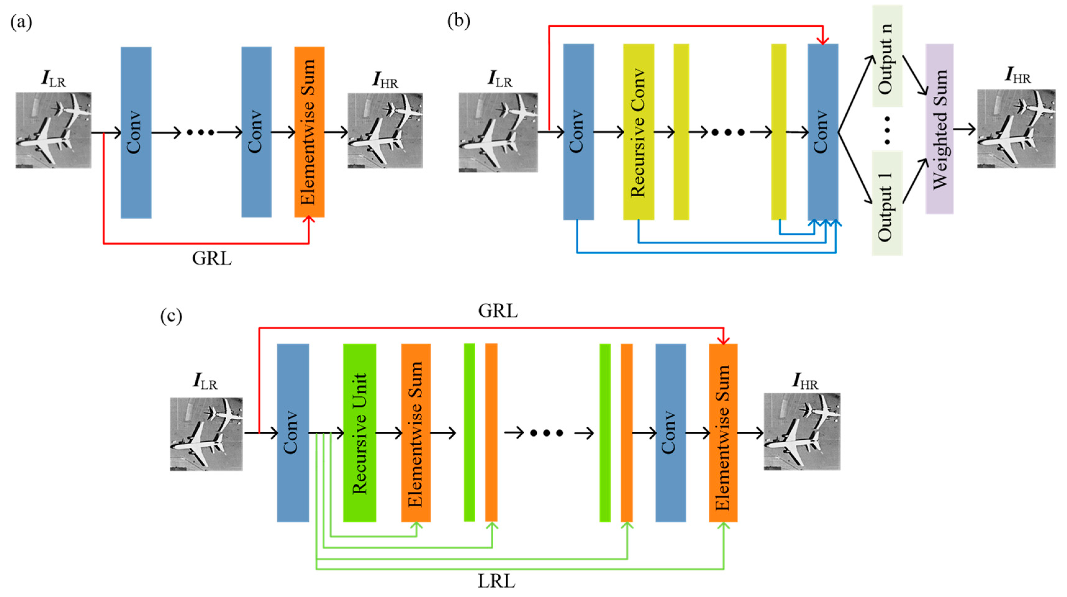
2.2. Residual Learning-Based SR

Originally, residual learning was proposed to address problems such as image classification and detection. Residual learning exhibits excellent performance in computer vision problems from low-level to high-level tasks. Christian et al. introduced the idea of residual learning into the problem of SR and employed a deep residual (Res-Net) with skip-connection as the GN, as shown in Figure 1. Res-Net utilizes local residual learning (LRL) to ease the training of networks, and comprehensive empirical evidence showed that the residual networks are easier to optimize and able to gain accuracy from the considerably increased depth. Nevertheless, LRL simply extracts local features by preserving the information, and it is not able to save the hierarchical features in a global manner.

Kim et al. [42] were enlightened by the residual network and then introduced a deeper network for super-resolution (VDSR), as shown in Figure 3a. It should be noted that the layers with the same color in Figure 3 belong to the same class. VDSR increased the network depth via cascading, vast convolutional layers. Since the reconstructed HR image is very similar to the input, global residual learning (GRL) is effective at reducing the difficulty of training deep networks. Kim et al. [43] augmented the receptive field of the network by introducing a recurrent neural network (DRCN), as shown in Figure 3b, which is beneficial for parameter sharing and reducing memory consumption. Moreover, they utilized recursive-supervision and skip-connection to overcome the difficulty of training. Tai et al. [44] proposed a very deep convolutional neural network model named deep recursive residual network (DRRN, illustrated in Figure 3c) that strives for deep yet concise networks. DRRN adopts both GRL and LRL. GRL and LRL mainly differ in that LRL is performed in every few stacked layers, while GRL is performed between the input and output images. Particularly, both GRL and LRL are employed to ease the problem of training the deep network. Comprehensive empirical evidence shows that the residual networks are easier to optimize and able to gain accuracy from their considerably increased depth. In contrast to residual learning-based SR methods, GAN-based approaches can recover more convincing and realistic HR images.

3. Proposed Method

In this section, we first describe the designed GN in the proposed dense residual generative adversarial network (DRGAN) in detail. Then, we demonstrate the DN part. Finally, we explicitly introduce the modified loss function of DRGAN according to WGAN-GP.

In this paper, let $I_G$ denote the ground-truth image with size m × n. $I_L$ denotes the down-sampled result of $I_G$ with size (m/s) × (n/s), where s is the corresponding scale factor. $I_{SR}$ represents the corresponding reconstructed SR image with size m × n.

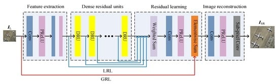
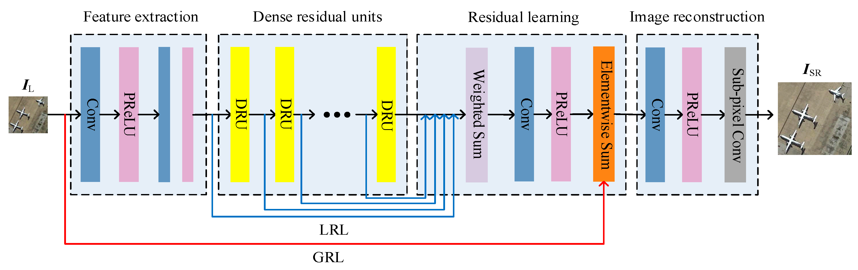
3.1. Structure of the GN

The whole architecture of the GN is drawn in Figure 4. According to the functions in the GN, we can divide it into four parts: feature extraction, dense residual units (DRUs), residual learning and image reconstruction. $I_L$ and $I_{SR}$ are the input and output of the GN, respectively. Nah et al. removed the batch normalization layers in their image deblurring work due to the batch normalization layers normalizing the features and getting rid of range flexibility [45]. That is to say, the batch normalization layers are applicable in the area of target classification rather than the field of SR. Therefore, we did not employ batch normalization (BN) layers in the whole GN, as shown in Figure 4.

3.1.1. Feature Extraction

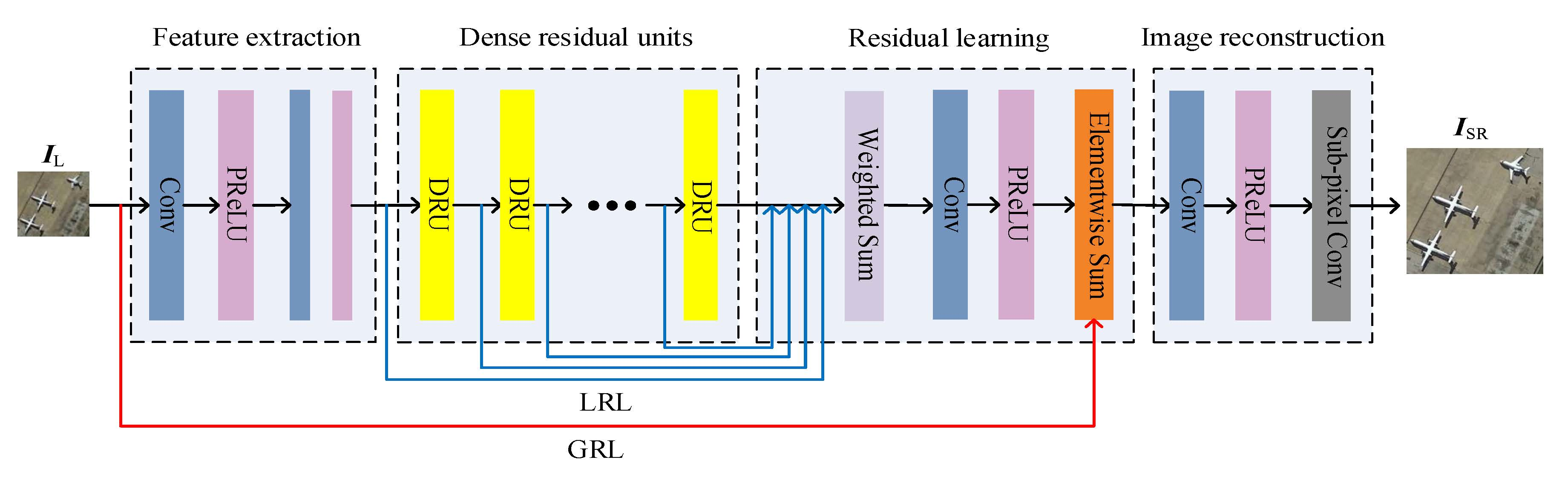
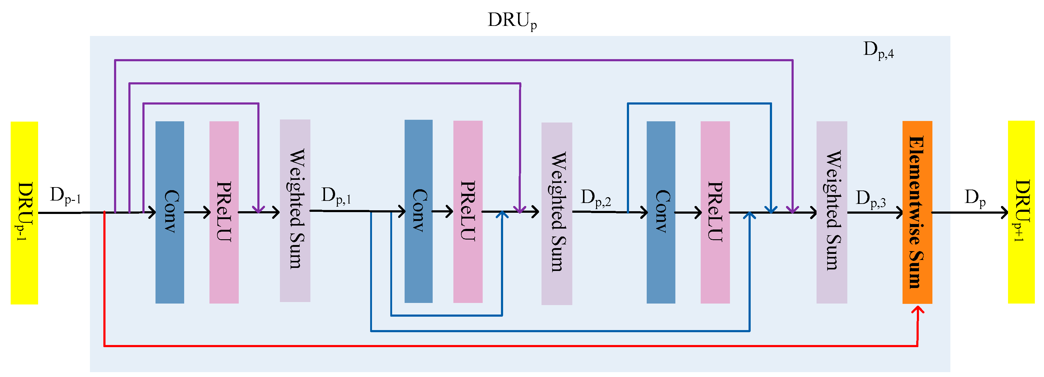
We employed two convolutional layers to extract features at first, because of two significant roles of convolutional layers: mitigating the effect of noise and strengthening the characteristics of the original signal. The operation of the feature extraction part can be expressed as follows:

$$\{\begin{array}{c}{F}_1=g\left(W_{FE,1}\ast I_L+B_{FE,1}\right)\\ FE=g\left(W_{FE,2}\ast F_1+B_{FE,2}\right)\end{array},$$

(1)

where $W_{FE,1}$ and $W_{FE,2}$ represent $n_{FE,1}$ convolution kernels of size $c\times k_{FE,1}\times k_{FE,1}$ and $n_{FE,2}$ convolution kernels of size $n_{FE,1}\times k_{FE,2}\times k_{FE,2}$, respectively; c denotes the channel number of the input image $I_L$; $k_{FE,1}$ and $k_{FE,2}$ are the spatial sizes of the convolution filter; $B_{FE,1}$ and $B_{FE,2}$ represent the biases; $\ast$ represents the convolution operation; $g(\cdot )$ represents the activation function; and $FE$ is the output part of the feature extraction and the input of the DRU.

In the case of SR, we only need to process the luminance channel of images, since human eyes are more sensitive to the brightness information of the images. Thus, we extract the Y-channel after transforming the images from RGB to YC_bC_r color space. The remaining two channels are upscaled to the required size via bicubic interpolation, and the final SR image can be obtained by fusing these three channels of the image. Therefore, the channel number of the input image $I_L$ is always c = 1.

This paper adopts the parametric rectified linear unit (PReLU) [46] as the activation function g(·). It can achieve a regular effect to a certain extent. Compared to ReLU [47], PReLU improves the convergence rate of the network by adding a few of parameters. The formula of g(·) can be expressed as follows:

$$g\left(x\right)=\{\begin{array}{c}x,\\ {\alpha }_{t}x,\end{array}\begin{array}{c}\\ \end{array}\begin{array}{c}if x>0\\ if x<0\end{array},$$

(2)

where ${\alpha }_t$ is a learnable parameter, $\alpha$ is initialized to 0.25 and $t$ denotes the time of iteration. When the network updates the parameters in reverse, the update formula of ${\alpha }_t$ can be formulated as

$$\Delta {\alpha }_{t+1}=\mu \Delta {\alpha }_t+\epsilon \frac{\partial L}{\partial {\alpha }_t},$$

(3)

where $\mu$ denotes the momentum, $\epsilon$ refers to the learning rate and $L$ represents the loss function.

3.1.2. DRUs

Assume that there are d DRUs; the specific architecture of each DRU is shown in Figure 5. Each DRU includes three convolutional layers, three activation layers, one weighted-sum layer and one element-wise sum layer. The convolutional layers in each DRU are densely connected in the manner shown in Figure 5. GRL and LRL are utilized simultaneously.

The whole operation of p-th DRU_p can be formulated as follows:

$$\{\begin{array}{c}{D}_{p,1}=S_{p,1}\left(g\left(W_{p,1}\ast D_{p-1}+B_{p,1}\right),D_{p-1}\right)\\ \begin{array}{c}\begin{array}{c}{D}_{p,2}=S_{p,2}\left(g\left(W_{p,2}\ast D_{p-1}+B_{p,2}\right),D_{p,1},D_{p-1}\right)\\ D_{p,3}=S_{p,3}\left(g\left(W_{p,3}\ast D_{p-2}+B_{p,3}\right),D_{p,2},D_{p,1},D_{p-1}\right)\end{array}\\ D_p=D_{p,3}+D_{p-1}\end{array}\end{array}$$

(4)

where $W_{p,1}$ to $W_{p,3}$ and $B_{p,1}$ to $B_{p,3}$ represent the kernels and biases, respectively, of the three successive convolutional layers; $S_{p,1}$ to $S_{p,3}$, denote the weighted-sum layers in sequence; $D_{p,1}$ to $D_{p,3}$ represent the output of the former convolutional layers in sequence (the activation layers are omitted for clarity); and $D_p$ denotes the corresponding output of the p-th DRU_p.

The blue lines in Figure 5 represent that the preceding outputs of convolutional layers in a DRU are fed into the posterior convolutional layers, which form the short-term memory. Similarly, the red and purple lines in Figure 5 represent that the preceding outputs of DRUs are fed into the latter layers, which correspond to the long-term memory. The outputs of the previous DRUs and convolutional layers can connect to the latter layers directly, which can not only save the feed-forward features but also extract local dense features. All of these result in a memory mechanism.

In the circumstance that the former DRU and the whole convolutional layers are fed into the latter layer, we need to decrease the feature numbers to reduce the burden of the network. Thus, we employ weighted-sum layers $S_{p,1}$ to $S_{p,3}$ that adaptively learn specific weights for each memory, which determines how much of the long-term and short-term memory should be saved. We refer to the operation of $S_{p,1}$ to $S_{p,3}$ in DRU_p as the local decision function.

3.1.3. Residual Learning

In recent studies, residual networks have achieved great performance on the low-level to high-level computer vision tasks. In this paper, we adopt both LRL and GRL in order to make full use of them. As shown in Figure 5, the blue lines represent LRL for the GN, and the red lines denote GRL for GN. The whole function of the part of residual learning can be formulated as follows:

$$\{\begin{array}{c}{R}_{ws}=S_{RL}\ast \left(D_1,D_2,\cdots ,D_d,FE\right)\\ R_{ws,1}=g\left(W_{RL,1}\ast R_{ws}+B_{RL,1}\right)\\ R=R_{ws,1}+F_1\end{array},$$

(5)

where $S_{RL}$ denotes the weighted-sum layer; $W_{RL,1}$ and $B_{RL,1}$ represent the kernel and bias, respectively, of the convolutional layer; $D_1$ to $D_d$ represent the outputs of the d DRU successively; and $R_{ws}$, $R_{ws,1}$ and $R$ denote the outputs of the weighted-sum layer, the convolutional layer and the element-wise sum layer in the part of residual learning, respectively.

The difference between LRL and GRL in the part of residual learning is that LRL is acquired between the DRU and the weighted-sum layer, while GRL is implemented between the input image $I_L$ and the element-wise sum layer, as shown in Figure 5. The weighted-sum layer $S_{RL}$ is used to extract the hierarchical features obtained from the previous DRUs through LRL and to decide their proportions in the ensuing features. We define the operation of $S_{RL}$ in the part of residual learning as the global decision function compared to $S_{p,1}$ to $S_{p,3}$ in DRU_p. The convolutional layer W_RL,1 is employed to further exploit features, and the element-wise sum layer aims for the GRL. The combination of LRL and GRL improves the performance of the GN and is less prone to over-fitting.

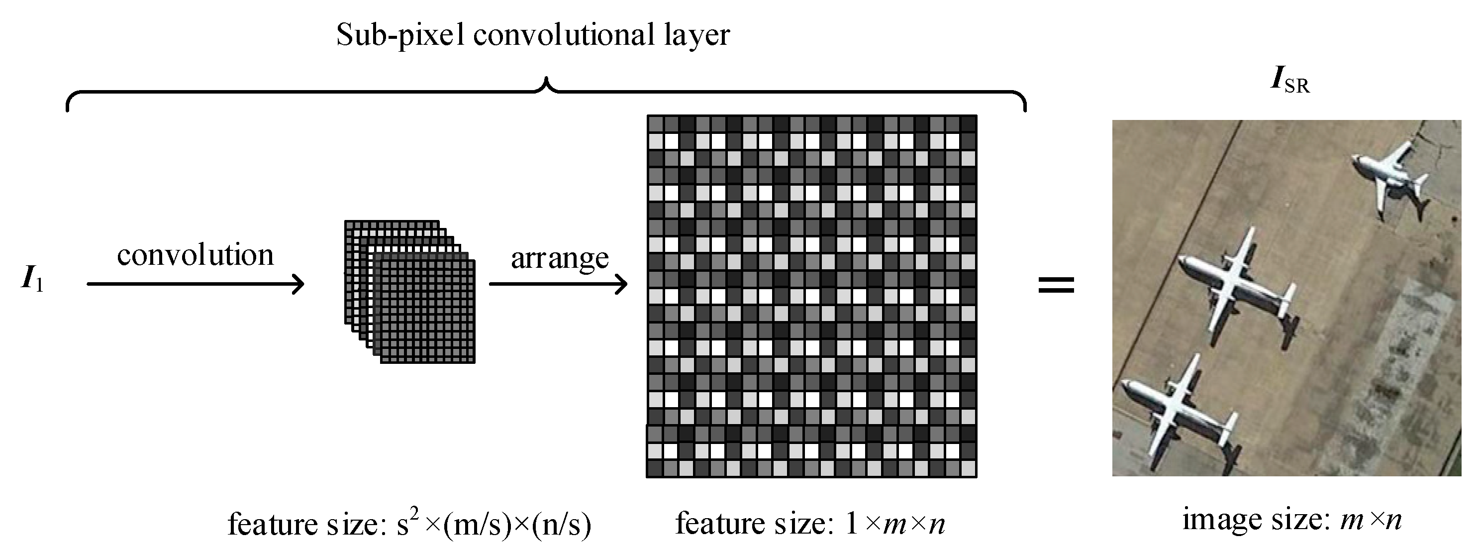
3.1.4. Image Reconstruction

Inspired by ESPCN, we adopted a sub-pixel convolutional layer for image upscaling and reconstruction in addition to a convolutional layer. The whole function of the part of image reconstruction can be formulated as follows:

$$\{\begin{array}{c}{I}_1=g\left(W_{IR,1}\ast R+B_{IR,1}\right)\\ I_{SR}=I=W_{IR,sc}\ast I_1\end{array},$$

(6)

where $W_{IR,1}$ and $B_{IR,1}$ represent the kernel and bias, respectively, of the convolutional layer; $W_{IR,sc}$ denotes the sub-pixel convolutional layer; $\ast$ denotes the operation of sub-pixel convolution; $I_1$ and $I$ denote the outputs of the convolutional layer and the sub-pixel convolutional layer in the part of image reconstruction; and $I$ is the final SR image obtained, $I_{SR}$.

The sub-pixel convolution layer $W_{IR,sc}$ can be conceptually separated into two steps, and the conceptual graph is shown in Figure 6:

1)

Convolution. Similar to the previous convolution layers in the GN, this step is used to extract features. The difference between them is that there are $s^2$ feature maps according to the upscaling factor $s$.

2)

Arrangement. Arrange all the pixels in the corresponding position of $s^2$ feature maps in a predetermined order in order to combine them into a series of areas. The size of each area is $s\times s$. Each area corresponds to a mini-patch in the final SR image $I_{SR}$. In this manner, we rearrange the final feature maps of size $s^2\times \left(m/s\right)\times \left(n/s\right)$ into $I_{SR}$ of size $1\times m\times n$. This implementation equals the rearrangement of the image without convolution operations, and thus, requires very little time.

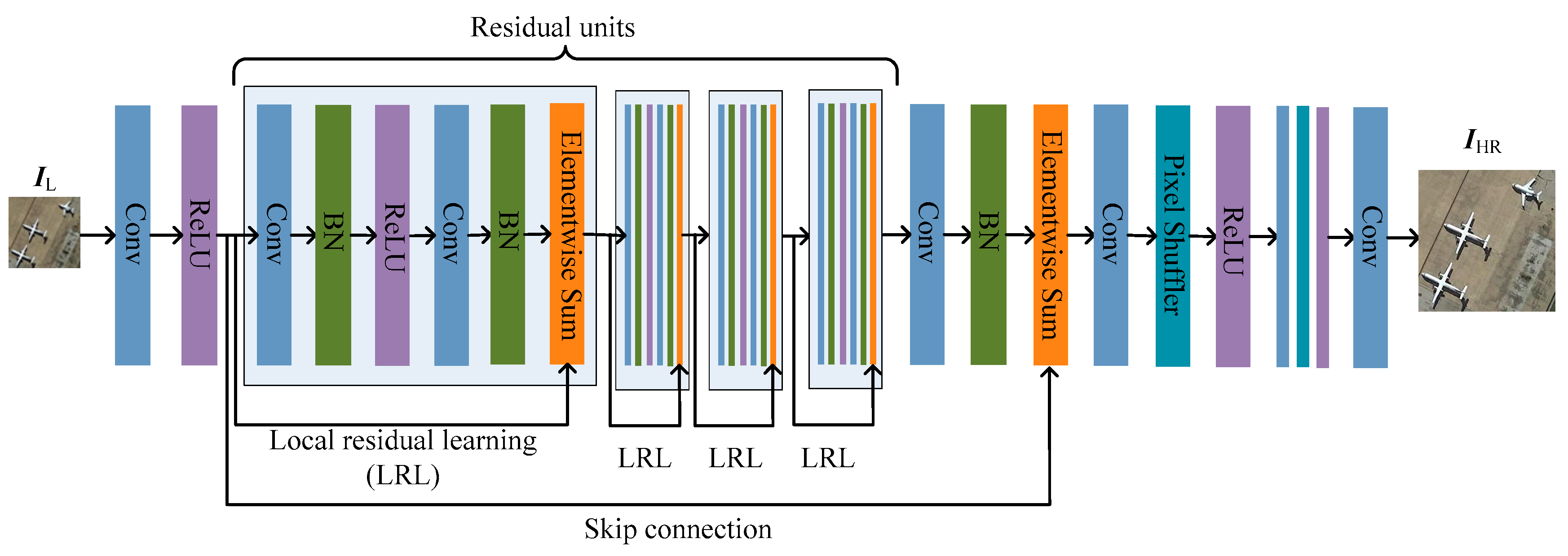
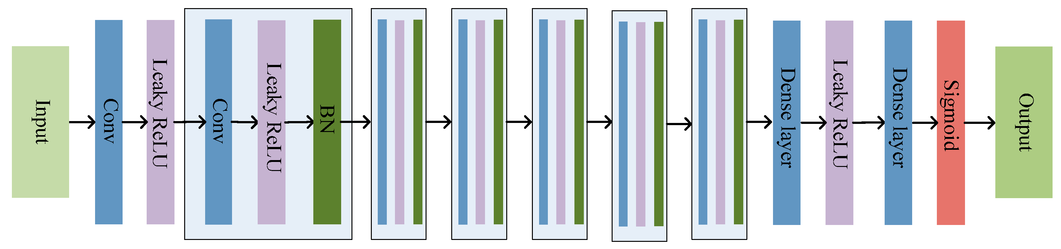
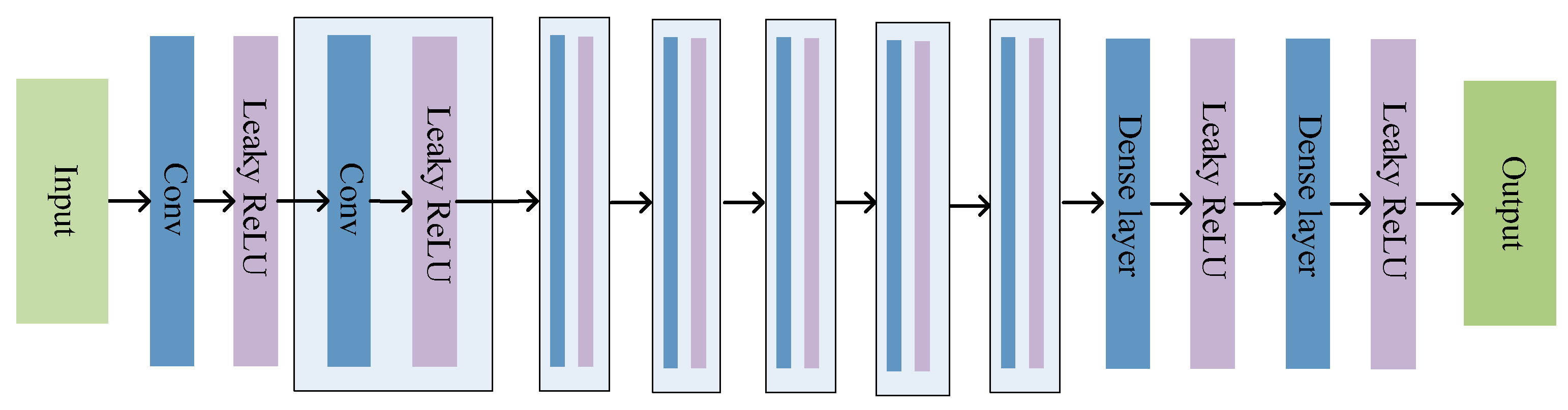
3.2. Structure of the DN

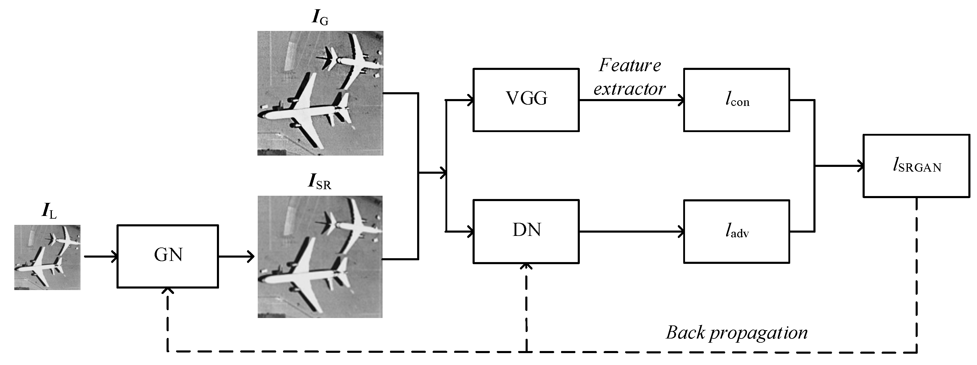
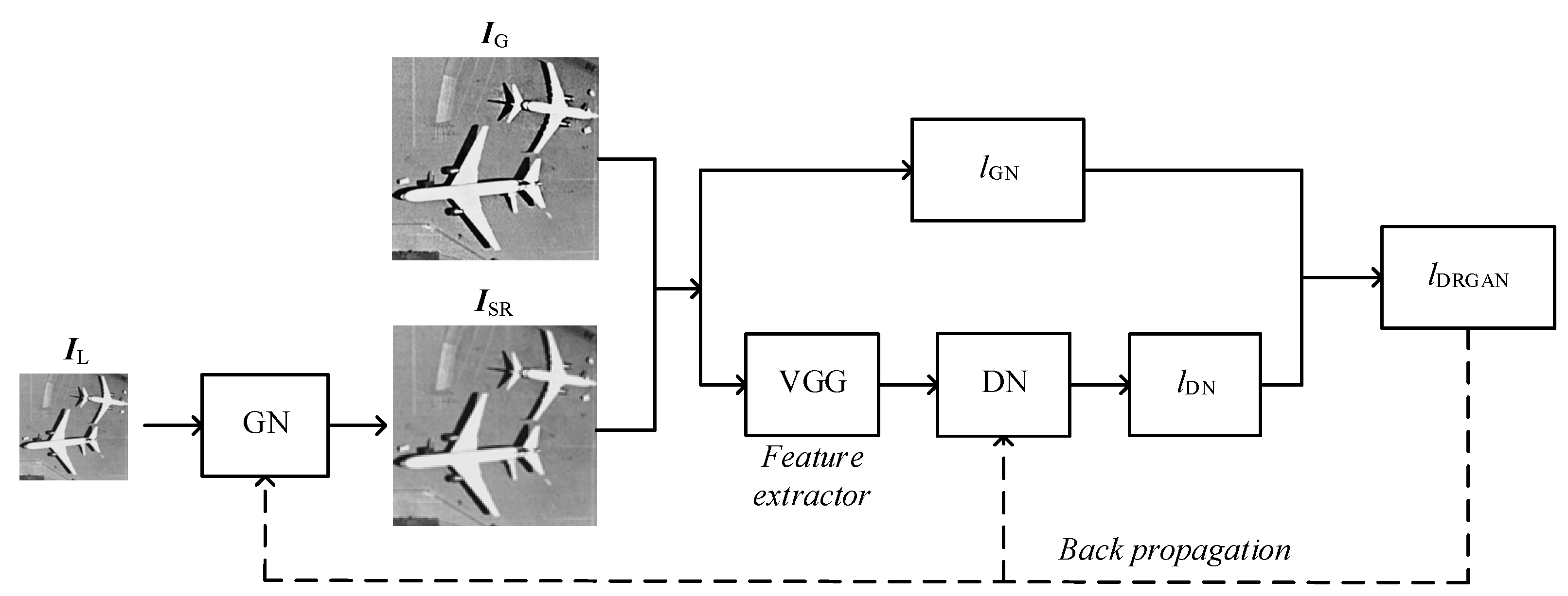
According to the theory of GANs, there is a DN in addition to the GN, which forms the adversarial networks: the GN produces the reconstructed image $I_{SR}$, while the DN is used to distinguish between the ground-truth image $I_G$ and $I_{SR}$. That is to say, we should optimize the parameters ${\theta }_{DN}$ in the DN along with the parameters ${\theta }_{GN}$ in the GN in an alternating manner to solve the adversarial min-max problem:

$$\underset{{\theta }_{DN}}{\min } \underset{{\theta }_{GN}}{\max }{E}_{I_G~P_D}\left[\log {\theta }_{DN}\left(I_G\right)\right]+E_{I_{HR}~P_G}\left[1-\log {\theta }_{GN}\left(I_{HR}\right)\right].$$

(7)

where $P_D$ is the distribution of the ground-truth image and $P_G$ is the distribution of the reconstructed image.

With the advantages of the GAN, we can recover $I_{SR}$ that is highly similar to the ground-truth image $I_G$ and difficult to distinguish via the DN.

However, differently from the DN in SRGAN, as shown in Figure 2, we make modifications in terms of two aspects. First, we replace the last sigmoid layer with a Leaky ReLU layer referring to WGAN-GP. The discriminator in SRGAN mainly aims for the task of true and binary classification, while the purpose of the DN in DRGAN is fitting the distance of Wasserstein approximately. Second, we remove the BN layers in the DN. We apply a gradient penalty for each sample individually. However, BN layers in the DN will have undesirable effects on the gradient penalty for the reason that BN layers may introduce interdependent relationships among different samples in the same batch. Thus, we omit the BN layers. The final architecture of the DN is shown in Figure 7.

3.3. Loss Function

In SRGAN, the perceptual loss function $l_{SRGAN}$ was proposed, and it was the weighted sum of a content loss $l_{con}$ and an adversarial loss $l_{adv}$. The conceptual process of training SRGAN is shown in Figure 8. $l_{SRGAN}$ is formulated as follows:

$$l_{SRGAN}=l_{con}+{10}^{-3}{l}_{adv}.$$

(8)

Specifically, $l_{con}$ is defined as the Euclidean distance between the feature maps of the recovered image ${\theta }_{GN}\left(I_L\right)$ and the corresponding ground-truth image $I_G$ in VGG, and it is formulated as

$$l_{con}=\frac{1}{w_{j,k}{h}_{j,k}}{\displaystyle \sum _{x=1}^{w_{j,k}}{\displaystyle \sum _{y=1}^{h_{j,k}}{\left[f_{j,k}{\left(I_G\right)}_{x,y}-f_{j,k}{\left({\theta }_{GN}\left(I_L\right)\right)}_{x,y}\right]}^2}},$$

(9)

where $f_{j,k}$ is the feature map acquired from the k-th convolutional layer before the j-th pooling layer in the VGG, and $w_{j,k}$ and $h_{j,k}$ denote the dimensions of the respective feature maps.

VGG is taken as a universal feature extractor to extract high-level features. $l_{con}$ is equal to the MSE between the high-level features extracted by VGG. With the advantage of $l_{con}$, the reconstructed images become more realistic and full of abundant details.

Besides the content loss, SRGAN also introduced the adversarial loss in order to promote the network to favor solutions that reside on the manifold of ground-truth images by aiming to fool the DN. The adversarial loss is obtained from the result of ${\theta }_{DN}\left({\theta }_{GN}\left(I_L\right)\right)$ overall training samples as

$$l_{adv}=-\log {\theta }_{DN}\left({\theta }_{GN}\left(I_L\right)\right),$$

(10)

where ${\theta }_{DN}\left({\theta }_{GN}\left(I_L\right)\right)$ denotes the probability of judging the recovered image ${\theta }_{GN}\left(I_L\right)$ as the corresponding $I_G$. Furthermore, Equation (10) is transformed into Equation (11) for better gradient behavior.

$$l_{adv}=\log \left[1-{\theta }_{DN}\left({\theta }_{GN}\left(I_L\right)\right)\right]$$

(11)

However, in this paper, according to WGAN-GP, we modify the loss function $l_{DRGAN}$ of the proposed DRGAN to solve the problems of unstable training, gradient disappearing or exploding and mode collapse. The method of WGAN-GP was used to train our model, thereby solving the problem of gradient explosion during training via a new Lipschitz continuous limit method, the gradient penalty. For this reason, we omit the BN layers in the DN, as mentioned above. BN layers may introduce the interdependent relationships among different samples in the same batch. Moreover, the loss function based on the MSE of pixel space is supplemented, and the DN is used to discriminate the feature maps of $I_{SR}$ and $I_G$ extracted via VGG. In this manner, we can not only achieve convincing reconstructed images with abundant details but also acquire results with high PSNRs. The corresponding process of training the proposed DRGAN is shown in Figure 9.

Let $l_{GN}$ represent the loss function of GN and $l_{DN}$ denote the loss function of DN. Different from $l_{con}$ in SRGAN, $l_{GN}$ is formulated as

$$l_{GN}=\frac{1}{mn}{\displaystyle \sum _{x=1}^m{\displaystyle \sum _{y=1}^n{\left[{\left(I_G\right)}_{x,y}-{\left({\theta }_{GN}\left(I_L\right)\right)}_{x,y}\right]}^2}},$$

(12)

where $l_{GN}$ is the MSE between the reconstructed image $I_{SR}$ and the corresponding ground-truth image $I_G$ in VGG. Because of the content loss, the MSE loss provides solutions with the highest PSNR values, which are, however, perceptually rather smooth and less convincing than results achieved with a loss component that is more sensitive to visual perception.

How $l_{DN}$ differs from $l_{adv}$ in SRGAN, as shown in Equation (10), is reflected in three aspects. First, the DN is no longer used to distinguish the reconstructed image $I_{SR}$ and the corresponding ground-truth image. VGG extracts the high-level feature maps of $I_{SR}$ and $I_G$, which need to be distinguished by the DN in our DRGAN. Second, the result of ${\theta }_{DN}\left({\theta }_{GN}(·)\right)$ is acquired without logarithm operations. The reason for this choice is that the probability of distinguishing the fake from the real data is replaced with the Wasserstein distance between the distributions of ground-truth images and reconstructed images. The DN in DRGAN removes the last sigmoid layer. Third, the gradient penalty is supplemented to keep the gradient steady in the process of back-propagation. The loss function $l_{DN}$ of DN can be formulated as

$$l_{DN}={\theta }_{DN}\left(f\left({\theta }_{GN}\left(I_L\right)\right)\right)-{\theta }_{DN}\left(f\left(I_G\right)\right)+\lambda {\left[{\Vert {\nabla }_z{\theta }_{DN}\left(z\right)\Vert }_2-1\right]}^2$$

(13)

where $f\left({\theta }_{GN}\left(I_L\right)\right)$ and $f\left(I_G\right)$ represent the feature maps of $I_{SR}$ and $I_G$ extracted by VGG; ${\left[{\Vert {\nabla }_z{\theta }_{DN}\left(z\right)\Vert }_2-1\right]}^2$ is the gradient penalty according to WGAN-GP; $\lambda$ is the coefficient set to 10 based on several comparative experiments; and ${\nabla }_z$ indicates the operation of partial derivatives for $z$, which can be formulated as

$$z=\beta f\left(I_G\right)+\left(1-\beta \right)f\left({\theta }_{GN}\left(I_L\right)\right), \beta ~uniform\left[0,1\right].$$

(14)

The whole process of training the proposed DRGAN can be divided into five steps:

1)

Feed the LR image $I_L$ into the GN, obtain the corresponding reconstructed image $I_{SR}$ and compute the content loss $l_{GN}$ based on the MSE.

2)

Import the reconstructed image $I_{SR}$ and the corresponding ground-truth image $I_G$ into VGG, and extract the respective high-level features.

3)

Feed the extracted feature maps into the DN and obtain the adversarial loss. The final loss is computed as the weighted sum of the content loss $l_{GN}$ and the adversarial loss $l_{DN}$.

4)

Implement the backward process of the network and compute the gradients of each layer. Optimize the network iteratively by updating the parameters in the DN and GN according to the training policy.

5)

Repeat the above steps until reaching the minimum loss of the network, and then the work of training the network is finished.

In this paper, the loss function that we proposed can show the training situation better than an ordinary GAN. Moreover, the gradient penalty can be reversed to the GN and the DN to minimize the loss of the generated network $l_{GN}$ and maximize the loss of the discriminating network $l_{DN}$.

4. Experiments

In this section, we first describe the preparation for the experiments. Then, we illustrate the details of the implementation and introduce two quality evaluation indexes for images that are commonly used in the related literature.

4.1. Dataset

NWPU-RESISC45 [48] is a classical scene classification data set consisting of remote sensing images 256 × 256 pixels in size. NWPU-RESISC45 contains 45 types of ground features in total, with 700 images per type. In this study, we chose the series of airplane images as targets and selected 500 airplane images as the objective training sample, while leaving 100 images for validation images and the rest as test images.

4.2. Training Details

Referring to WGAN-GP, we adopt RMSprop [49] rather than Adam [50] to optimize our model; the weight matrices W are updated as

$${\left(v_t\right)}_q={\{{\begin{array}{c}{\left(v_{t-1}\right)}_q+\delta ,\\ {\left(v_{t-1}\right)}_q·\left(1-\delta \right),\end{array}}_{}}_{}^{}{}_{}\begin{array}{c}{\left(\nabla L\left(W_t\right)\right)}_q{\left(\nabla L\left(W_{t-1}\right)\right)}_q>0\\ else\end{array},$$

(15)

$${\left(W_{t+1}\right)}_q={\left(W_t\right)}_q-\epsilon {\left(v_t\right)}_q,$$

(16)

where $\delta$ is initialized to 0.02, W denotes the weights in the network, $q$ denotes the order of the element in W, $v$ represents an adaptive moment estimation, t denotes the iteration time and the learning rate $\epsilon$ is initialized to 0.0001.

Before training, we augment the remote sensing images by horizontally flipping and rotating. Then, we down-sample the ground training images $I_G$ by the required upscale factor s to obtain the LR images $I_L$. For each mini-batch, we cropped 16 random sub images from LR training samples of size 64 × 64 and sub images from ground-truth training samples of size 256 × 256. Taking considerations of both training time and complexities of the network, we employed eight dense recursive units in the GN described in Section 3.1. Each convolutional layer in the GN owns a 3 × 3 kernel and 64 feature maps. Moreover, we adopted zero padding in each convolutional layer to make sure the outputs had the same sizes as the original inputs.

We implemented the experiments in TensorFlow [51] and accelerated them using a single NVIDIA GTX1080TI GPU with 11 GB of memory. Specifically, we first trained the GN with only the loss function based on $l_{GN}$, as formulated in Equation (12), and then we initialized the entire DRGAN network with it to avoid undesirable local optima. The whole process of training required approximately four days.

$$l_{MSE}=\frac{1}{mn}{\displaystyle \sum _{x=1}^m{\displaystyle \sum _{y=1}^n{\left[{\left(I_G\right)}_{x,y}-{\left({\theta }_{GN}\left(I_L\right)\right)}_{x,y}\right]}^2}}.$$

(17)

4.3. Quantitative Evaluation Factors

4.3.1. Peak Signal-To-Noise Ratio (PSNR)

The PSNR [52] was adopted in this paper as the quality evaluation index of the reconstructed HR image. It is dependent on the MSE between the ground-truth images $X=\left\{X_i\right\}$ and the reconstructed HR images $H=\left\{H_i\right\}$. The formulas for MSE and PSNR can be expressed as follows:

$$MSE=\frac{1}{mn}{\displaystyle \sum _{a=1}^m{\displaystyle \sum _{b=1}^n{\left(X_i(a,b)-H_i(a,b)\right)}^2}},$$

(18)

$$PSNR=10\lg \frac{{255}^2}{MSE},$$

(19)

where $m$ and $n$ denote the height and width of images $X_i$ and $H_i$; $a$ and $b$ represent the horizontal and vertical axes.

4.3.2. Structural Similarity Index (SSIM)

The SSIM [52] is commonly used for the evaluation of the quality of the reconstructed HR images, and it is calculated as follows:

$$SSIM\left(X_i,H_i\right)=c\left(X_i,H_i\right)d\left(X_i,H_i\right)e\left(X_i,H_i\right),$$

(20)

where $c\left(X_i,H_i\right)$ denotes the brightness contrast, $d\left(X_i,H_i\right)$ denotes the comparison of contrast, $e\left(X_i,H_i\right)$ represents the contrast of pixel structure and

$$\{\begin{array}{c}c\left(X_i,H_i\right)=\frac{2{\mu }_{X_i}{\mu }_{H_i}+C_1}{{\mu }_{X_i}^2+{\mu }_{H_i}^2+C_1}\\ d\left(X_i,H_i\right)=\frac{2{\sigma }_{X_i}{\sigma }_{H_i}+C_2}{{\sigma }_{X_i}^2+{\sigma }_{H_i}^2+C_2}\\ e\left(X_i,H_i\right)=\frac{{\sigma }_{X_i{H}_i}+C_3}{{\sigma }_{X_i}{\sigma }_{H_i}+C_3}\end{array},$$

(21)

where ${\sigma }_{X_i}^2$ and ${\sigma }_{H_i}^2$ denote the variance of images $X_i$ and $H_i$; ${\sigma }_{X_i{H}_i}$ refers to the covariance between $X_i$ and $H_i$; ${\mu }_{X_i}$ and ${\mu }_{H_i}$ indicate the average values of $X_i$ and $H_i$; and $C_1$, $C_2$ and $C_3$ are constants.

4.3.3. Normalized Root Mean Square Error (NRMSE)

The normalized root mean square error (NRMSE) used in [53] measures the distance between the data predicted by the mapping model and the original data observed from the environment. It can be computed as follows, and the smaller the value of NRMSE is, the better quality the reconstructed HR image has.

$$\mathrm{NRMSE}\left(\mathit{X},\mathit{H}\right)=\frac{\sqrt{\mathrm{MSE}\left(\mathit{X},\mathit{H}\right)}}{255}$$

(22)

4.3.4. Erreur Relative Globale Adimensionnelle De Synthese (ERGAS)

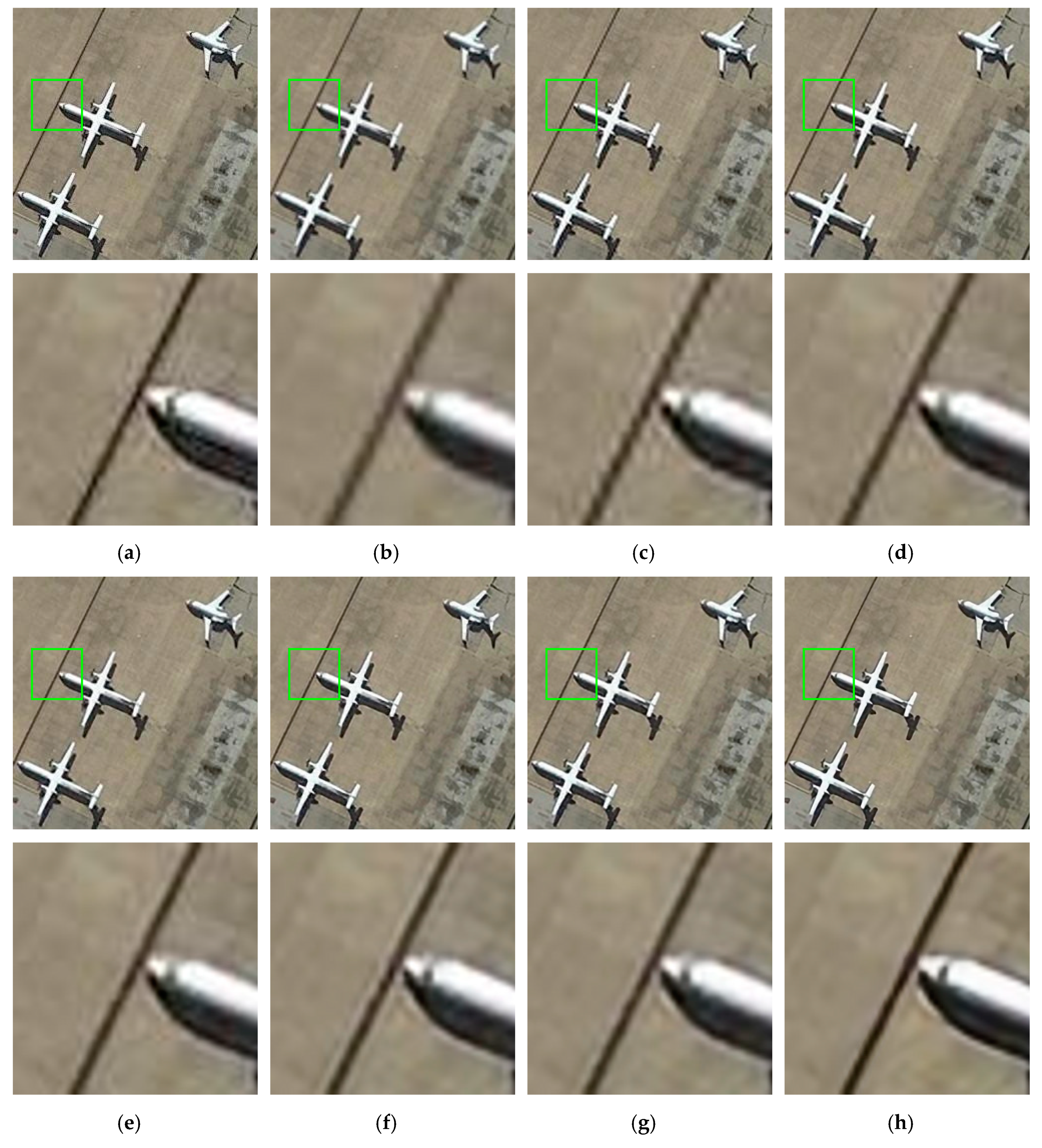
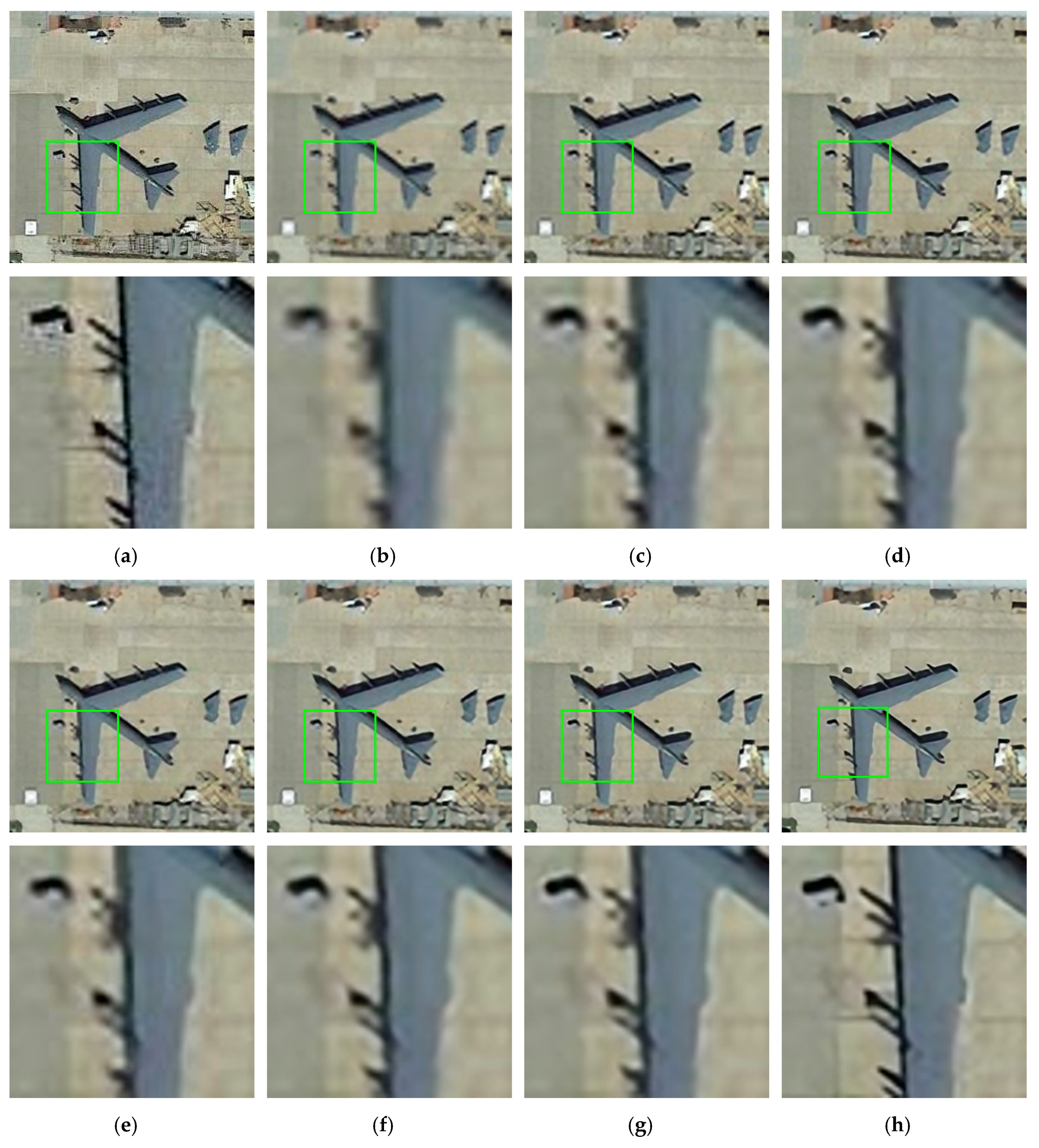
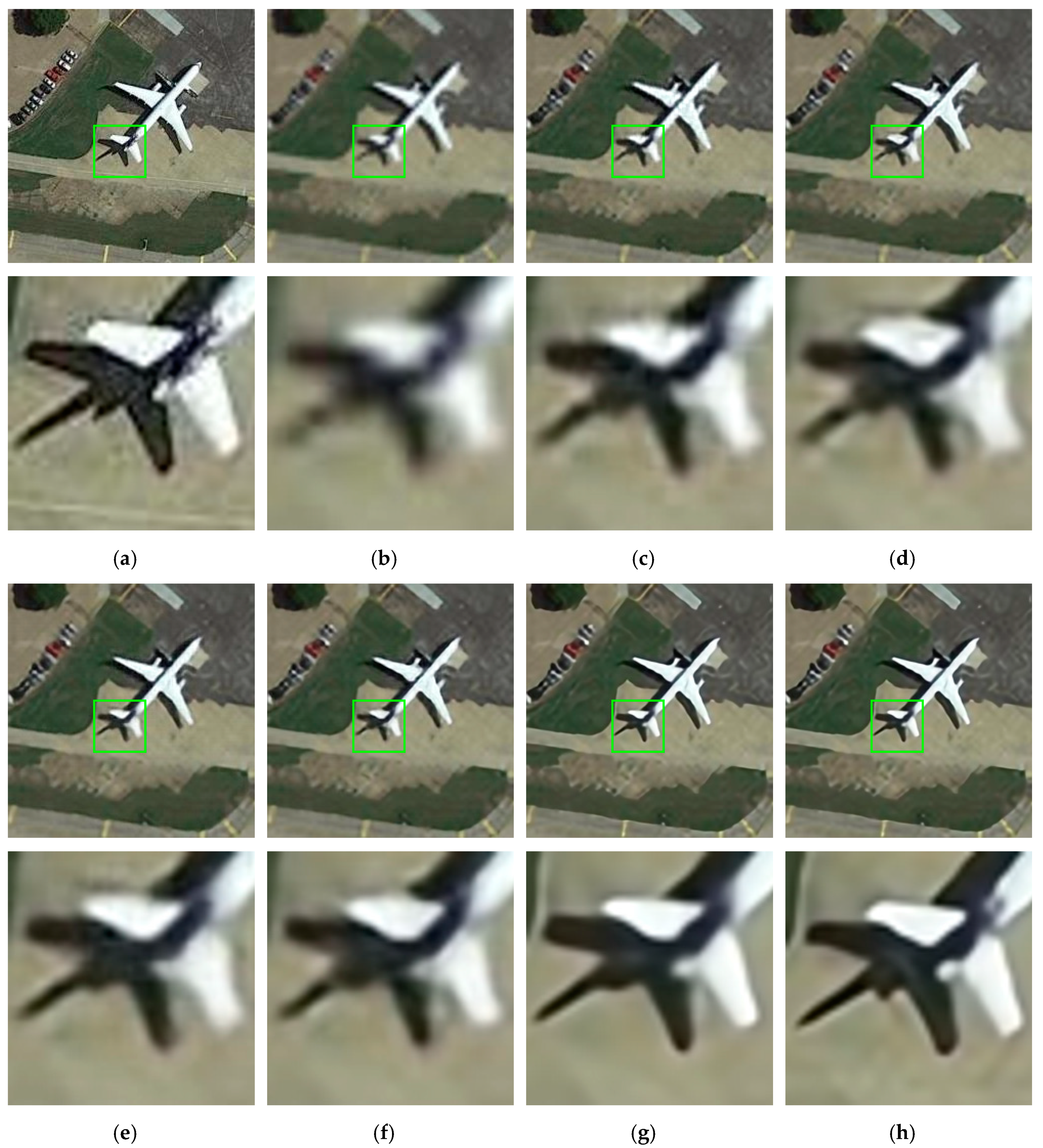
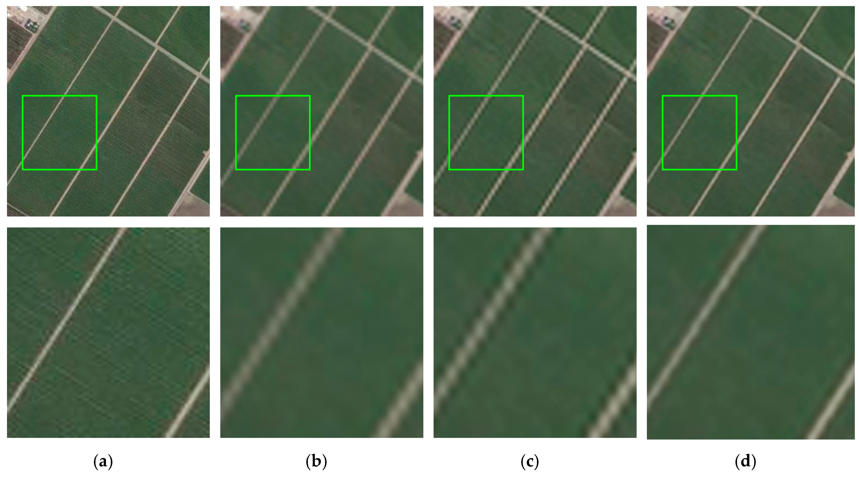
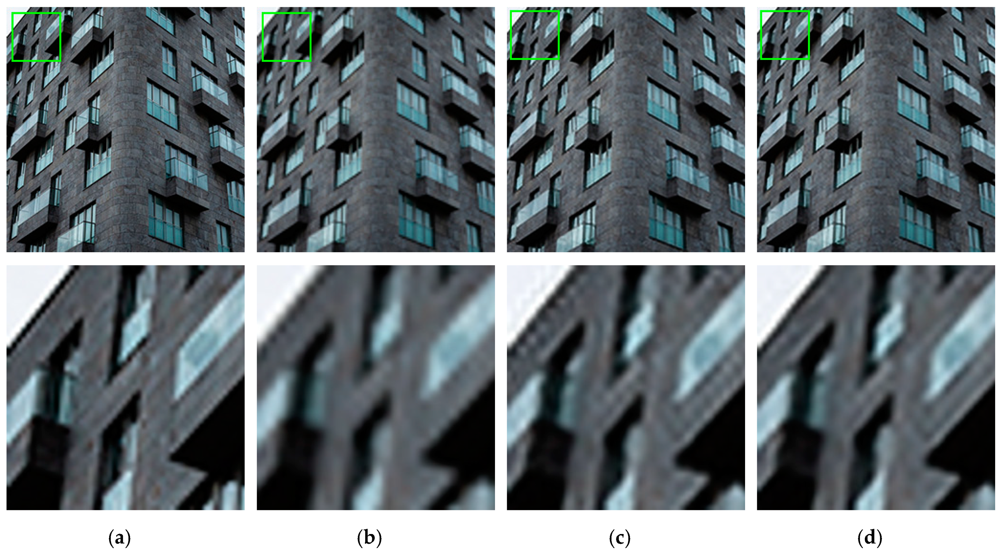
The erreur relative globale adimensionnelle de synthese (ERGAS) [54] was put forward to measure the quality of reconstructed HR images by taking the scaling factor into consideration, and it can be formulated as:

$$\mathrm{ERGAS}\left(\mathit{X},\mathit{H}\right)=\frac{100}{s}\sqrt{\frac{1}{c}{\left[\frac{\sqrt{\mathrm{MSE}\left(\mathit{X},\mathit{H}\right)}}{{\mu }_{\mathit{X}}}\right]}^2}$$

(23)

where s represents the scale factor, c denotes the channel number of the image, and ${\mu }_{\mathit{X}}$ is the mean value of $\mathit{X}$. The smaller the value of ERGAS, the better the quality of the reconstructed HR image.

5. Results

To test the performance of the proposed SR method via DRGAN, we implement tests in public datasets and compared the results of DRGAN with those of several state-of-the-art methods. In addition, we selected the results of bicubic interpolation as the baseline reference. For SISR methods based on DL, DRGAN was compared with SRCNN [20], FSRCNN [22], ESPCN [21], VDSR [42], DRRN [44] and SRGAN [34]. The publicly available testing codes from the corresponding authors were employed. For fair comparison, we cropped the pixels in the boundary before evaluation like the operation in SRCNN [20].

Table 1. Peak signal to noise ratio (PSNR) (dB) metric results for the NWPU dataset using different methods.

Title	Scale	Bicubic	SRCNN	FSRCNN	ESPCN	VDSR	DRRN	SRGAN	DRGAN (ours)
airplane _001	×2	29.99	32.85	33.72	33.23	34.14	34.34	-/-	34.62
	×3	26.95	28.84	29.59	29.21	30.29	30.45	-/-	30.69
	×4	25.21	26.45	26.94	26.68	27.66	27.88	26.25	28.11
airplane _035	×2	30.36	32.75	33.22	32.92	33.45	33.63	-/-	33.91
	×3	27.36	29.02	29.21	29.15	29.78	29.94	-/-	30.16
	×4	25.78	27.20	27.69	27.32	28.02	28.19	27.03	28.48
airplane _095	×2	27.98	29.86	30.36	30.08	30.69	30.86	-/-	30.15
	×3	25.34	26.54	26.95	26.80	27.31	27.54	-/-	27.80
	×4	24.02	24.87	25.11	25.00	25.36	25.53	24.69	25.83
Test dataset	×2	32.20	34.37	34.96	34.63	35.12	35.33	-/-	35.56
	×3	29.09	30.59	31.15	30.87	31.47	31.70	-/-	31.92
	×4	27.42	28.43	28.92	28.68	29.31	29.55	27.99	29.76

,

Table 2. Structural similarity index (SSIM) metric results for the NWPU dataset using different methods.

Title	Scale	Bicubic	SRCNN	FSRCNN	ESPCN	VDSR	DRRN	SRGAN	DRGAN (ours)
airplane _001	×2	0.9160	0.9489	0.9539	0.9515	0.9563	0.9583	-/-	0.9661
	×3	0.8350	0.8768	0.8893	0.8826	0.9013	0.9089	-/-	0.9196
	×4	0.7681	0.8035	0.8187	0.8111	0.8422	0.8512	0.8063	0.8622
airplane _035	×2	0.9401	0.9645	0.9697	0.9655	0.9709	0.9745	-/-	0.9811
	×3	0.8693	0.9074	0.9210	0.9101	0.9381	0.9396	-/-	0.9460
	×4	0.8053	0.8494	0.8676	0.8477	0.8950	0.9012	0.8554	0.9143
airplane _095	×2	0.8750	0.9152	0.9217	0.9190	0.9273	0.9338	-/-	0.9432
	×3	0.7708	0.8151	0.8307	0.8243	0.8444	0.8522	-/-	0.8628
	×4	0.7005	0.7369	0.7519	0.7460	0.7711	0.7802	0.7378	0.7908
Test dataset	×2	0.9042	0.9346	0.9397	0.9372	0.9435	0.9497	-/-	0.9631
	×3	0.8232	0.8582	0.8692	0.8644	0.8810	0.8904	-/-	0.9102
	×4	0.7623	0.7918	0.8045	0.7995	0.8240	0.8369	0.7933	0.8544

,

Table 3. Normalized root mean square error (NRMSE) metric results for the NWPU dataset using different methods.

Title	Scale	Bicubic	SRCNN	FSRCNN	ESPCN	VDSR	DRRN	SRGAN	DRGAN (ours)
airplane _001	×2	0.0317	0.0211	0.0206	0.0218	0.0196	0.0192	-/-	0.0186
	×3	0.0450	0.0362	0.0355	0.0346	0.0306	0.0300	-/-	0.0292
	×4	0.0549	0.0476	0.0449	0.0464	0.0414	0.0404	0.0487	0.0393
airplane _035	×2	0.0304	0.0230	0.0218	0.0226	0.0213	0.0208	-/-	0.0201
	×3	0.0429	0.0354	0.0334	0.0349	0.0324	0.0318	-/-	0.0310
	×4	0.0514	0.0437	0.0413	0.0431	0.0397	0.0389	0.0445	0.0377
airplane _095	×2	0.0399	0.0321	0.0303	0.0313	0.0292	0.0286	-/-	0.0311
	×3	0.0541	0.0471	0.0449	0.0457	0.0431	0.0420	-/-	0.0407
	×4	0.0629	0.0571	0.0555	0.0563	0.0539	0.0529	0.0583	0.0511
Test dataset	×2	0.0273	0.0215	0.0201	0.0209	0.0195	0.0171	-/-	0.0167
	×3	0.0382	0.0323	0.0304	0.0314	0.0293	0.0260	-/-	0.0254
	×4	0.0459	0.0408	0.0387	0.0398	0.0371	0.0333	0.0399	0.0325

,

Table 4. Erreur relative globale adimensionnelle de synthese (ERGAS) metric results for the NWPU dataset using different methods.

Title	Scale	Bicubic	SRCNN	FSRCNN	ESPCN	VDSR	DRRN	SRGAN	DRGAN (ours)
airplane _001	×2	3.6583	2.6447	2.3910	2.5311	2.2697	2.1977	-/-	2.0831
	×3	3.4587	2.7844	2.5551	2.6733	2.3535	2.2882	-/-	2.1940
	×4	3.1679	2.7466	2.5948	2.6816	2.3907	2.3011	2.6216	2.2354
airplane _035	×2	4.5529	3.4659	3.2829	3.3995	3.1908	3.1116	-/-	2.9958
	×3	4.3017	3.5533	3.3545	3.5144	3.2527	3.1998	-/-	3.0587
	×4	3.8641	3.2866	3.1039	3.2488	2.9900	2.8045	3.0587	2.7582
airplane _095	×2	4.0629	3.2816	3.0968	3.2021	2.9791	2.9877	-/-	2.8653
	×3	3.6805	3.2110	3.0617	3.1190	2.9353	2.9122	-/-	2.8800
	×4	3.2179	2.9187	2.8388	2.8827	2.7590	2.6654	2.8252	2.6029
Test dataset	×2	3.1608	2.5015	2.3451	2.4345	2.2666	2.2081	-/-	2.1630
	×3	2.9462	2.4996	2.3551	2.4379	2.2613	2.2475	-/-	2.1815
	×4	2.6522	2.3634	2.2415	2.3107	2.1469	2.0998	2.2973	2.0764

and

Table 5. Test time (s) results on NWPU dataset using different methods.

Title	Scale	Bicubic	SRCNN	FSRCNN	ESPCN	VDSR	DRRN	SRGAN	DRGAN (ours)
airplane _001	×2	0.0000	0.1297	0.0369	0.0319	1.7643	0.2157	-/-	0.1638
	×3	0.0000	0.1277	0.0189	0.0170	1.7264	0.2153	-/-	0.1619
	×4	0.0000	0.1287	0.0109	0.0120	1.7762	0.2154	0.7515	0.1610
airplane _035	×2	0.0000	0.1267	0.0339	0.0309	1.7513	0.2389	-/-	0.1820
	×3	0.0000	0.1316	0.0180	0.0170	1.7234	0.2374	-/-	0.1816
	×4	0.0000	0.1297	0.0100	0.0120	1.7563	0.2365	0.7550	0.1814
airplane _095	×2	0.0000	0.1316	0.0329	0.0299	1.7982	0.2268	-/-	0.0410
	×3	0.0000	0.1267	0.0160	0.0159	1.7254	0.2070	-/-	0.0382
	×4	0.0000	0.1466	0.0100	0.0100	1.7663	0.2099	0.7587	0.0394
Test dataset	×2	0.0000	0.1303	0.0337	0.0300	1.7961	0.2386	-/-	0.1621
	×3	0.0000	0.1278	0.0158	0.0156	1.7442	0.2173	-/-	0.1657
	×4	0.0000	0.1371	0.0096	0.0102	1.7689	0.2102	0.7647	0.1539

show the summarized results of PSNR, SSIM, NRMSE, ERGAS and test time, respectively, for three chosen images and the whole test datasets with three different upscaling factors (×2, ×3 and ×4). The proposed DRGAN outperforms all of the methods listen, in all scales, regardless of which metric is considered. At scale factors of ×2, ×3 and ×4, DRGAN boosts the second-best method by 0.23, 0.22 and 0.21 dB in PSNR, 0.0134, 0.0198 and 0.0175 in SSIM, 0.0004, 0.0006 and 0.0008 in NRMSE, and 0.0451, 0.0660 and 0.0234 in ERGAS. Moreover, although SRGAN can generate convincing results, the objective indicators of SRGAN do not compare well with those of other methods for the reason that its loss function is dependent on the feature space, not the pixel space.

It can be observed from Table 5 that when the number of convolutional layers of the network is relatively deep, such as in the models of VDSR, DRRN, SRGAN and the proposed DRGAN, the reconstruction time of the test image under our method is far less than that of other approaches.

In addition to the quantitative comparisons, we also performed visual comparisons among our method and above-listed methods. We show the reconstructed HR results with different scale factors in Figure 10, Figure 11 and Figure 12, and the ground-truth images are also provided for reference. For clearer contrast, we selected an area marked with a green rectangle to zoom in and placed the close-up below the corresponding whole image.

We show the SR results of ‘airplane_001.jpg’ with an upscaling factor ×2 in Figure 10. DRGAN accurately reconstructed straight lines and obtained clearer and sharper results than the other methods. It can be observed that the edges reconstructed by DRGAN are the clearest among all the approaches.

Figure 11 provides the reconstructed HR results of ‘airplane_095.jpg’ with a scale factor of ×3 and zoomed-in close-ups of the airplane wings. We can clearly observe that the edges of airplane wings in the images reconstructed by the other deep-learning-based methods are vaguer, relatively, or more distorted, while DRGAN achieves more convincing results with fewer artifacts. The edges resulting from the proposed DRGAN method are sharper and the contrasts are clearer than those of other state-of-the-art methods.

The reconstructed HR results of ‘airplane_035.jpg’ with a scale factor ×4 are shown in Figure 12. We also enlarged the area around the aircraft tail. We also display the results of SRGAN in Figure 12g. It is obvious that the reconstructed HR image obtained with DRGAN, which is shown in Figure 12h, is the best result that is closest to the ground-truth HR image shown in Figure 12a. We can see from the comparison that for a large-scale factor of ×4, the aircraft tail is reconstructed cleanly and vividly when using SRGAN and DRGAN, whereas it is blurred or distorted when using other methods, and DRGAN is better than SRGAN.

6. Discussion

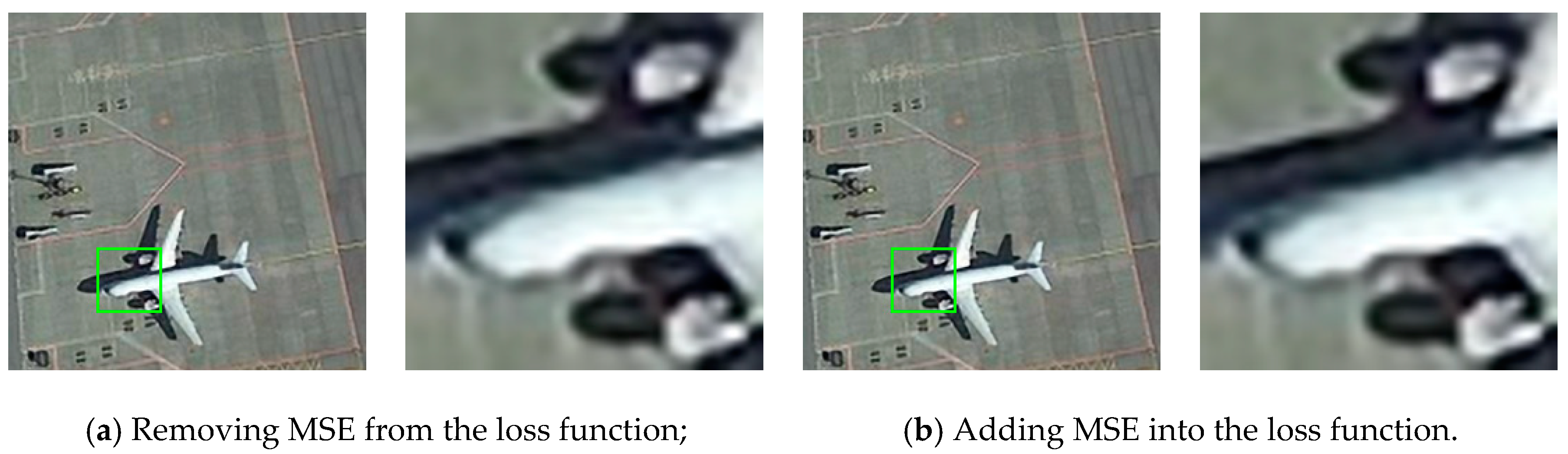
6.1. The Effect of Adding MSE into the Loss Function

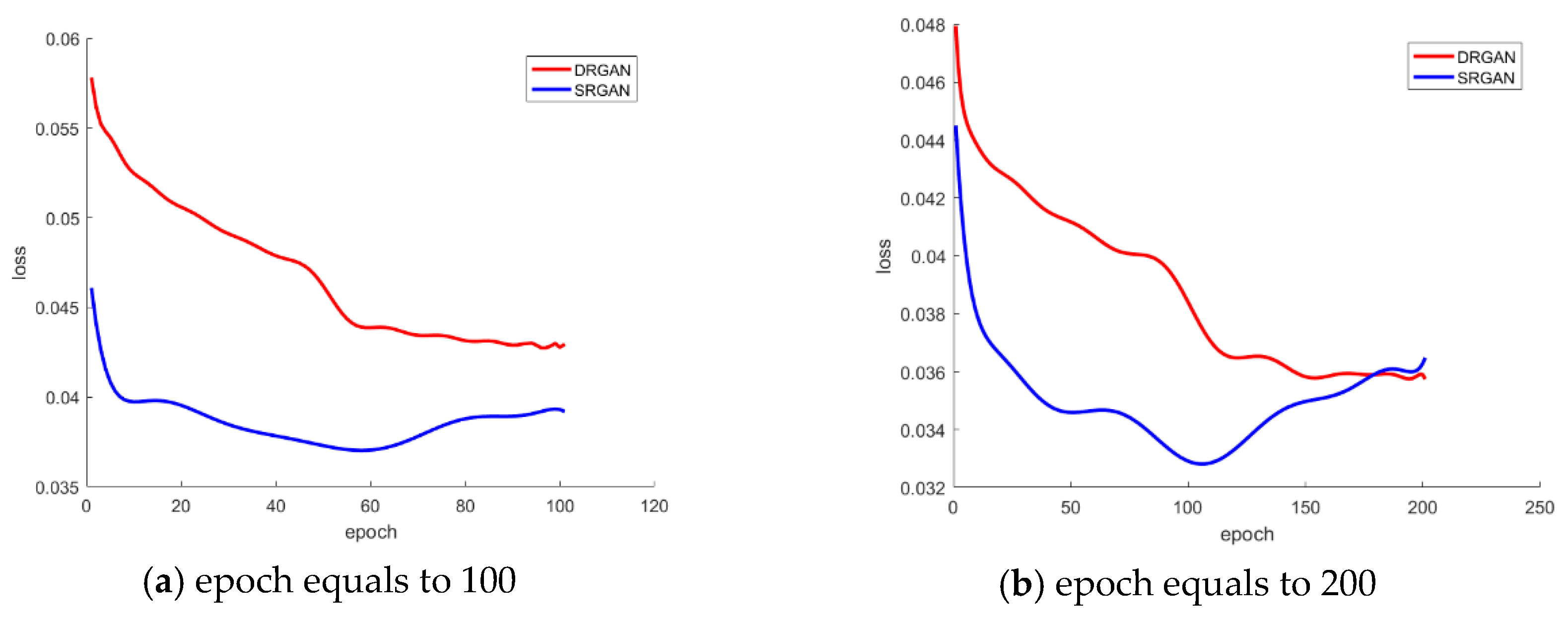
SRGAN’s perceptual loss, which consists of an adversarial loss and a content loss, can help the model generate convincing reconstructed results, but the objective indicators of SRGAN do not perform well against other methods because its loss function is dependent on the feature space, not the pixel space. To address this drawback, MSE loss was introduced in our proposed method to ensure the similarity between the output image and the target image.

To assess the effect of adding MSE loss, we compared the PSNR and SSIM values of reconstructed HR images obtained through the networks with and without MSE in the loss function with a scale factor of ×3 for the test set. The results indicate that the network with MSE loss added has superior performance relative to that without MSE constraint, and an improvement of approximately 0.36 dB in PSNR and 0.0085 in SSIM can be achieved using our new loss function.

Figure 13 compares the reconstructed HR images of ‘airplane_633.jpg’ obtained through the networks both excluding and including MSE in the loss function. It can be observed from the close-ups of the head of the airplane that the edges of the reconstructed image obtained from the network without the MSE constraint (as shown in Figure 13a) are much vaguer than those obtained from the network adding MSE loss (as shown in Figure 13b). Through testing on the whole test set, we found that the results obtained without MSE being constrained are more likely to generate artifacts, which proves that adding MSE loss can achieve more subjectively realistic visual effects.

6.2. The Impact of Using ${\mathcal{L}}_{gan}$ or ${\mathcal{L}}_{wgan}$ on Our SR Model

As is known, it is usually difficult to decide when to suspend the training of the generator or discriminator for traditional GAN-based approaches. GAN-based methods often suffer from the situation of gradient vanishing. As mentioned in Section 3, we referred to the key idea of WGAN-GP instead of using an ordinary GAN in our model.

For comparison, we drew the loss convergence curves of the generator of our model under the conditions of using ${\mathcal{L}}_{gan}$ or ${\mathcal{L}}_{wgan}$. We selected hyper parameter ‘epoch’ values of 100 and 200 and have displayed the experimental results. As shown in Figure 14, the red curves represent the trend of loss convergence under ${\mathcal{L}}_{wgan}$, while the blue curves represent the results of using ${\mathcal{L}}_{gan}$. It can be clearly observed from Figure 14a,b that the loss is difficult to converge (the blue curves) when using ordinary ${\mathcal{L}}_{gan}$ to train the model regardless of the hyper parameter ‘epoch’; after training for a period of time, the loss instead increases, which is called mode collapse and often occurs in GANs. Obviously, ${\mathcal{L}}_{wgan}$ can overcome this drawback very well. The curves of loss convergence of our model under ${\mathcal{L}}_{wgan}$ (the red curves) show that the loss is always decreasing until convergence is accomplished.

6.3. Robustness of the Model

To further test the performance of proposed SR reconstruction model, the DRGAN was tested using several natural image datasets (Set5 [55], Set14 [56], BSD100 [57], Urban100 [58]) and other types of remote sensing images besides those of airplanes.

Table 6. Objective metric results of several different methods using several natural datasets.

Title	Scale	BicubicPSNR/SSIM	SRCNNPSNR/SSIM	SRGANPSNR/SSIM	DRGANPSNR/SSIM
Set5	× 2	33.66/0.9299	36.66/0.9542	-/-	36.98/0.9602
	× 3	30.39/0.8682	32.75/0.9090	-/-	33.11/0.9130
	× 4	28.42/0.8104	30.49/0.8628	29.40/0.8472	30.86/0.8712
Set14	× 2	30.23/0.8687	32.45/0.9067	-/-	32.81/0.9118
	× 3	27.54/0.7736	29.30/0.8215	-/-	29.65/0.8286
	× 4	26.00/0.7019	27.50/0.7513	26.02/0.7397	27.89/0.7655
BSD100	× 2	29.56/0.8431	31.36/0.8879	-/-	31.91/0.8936
	× 3	27.21/0.7385	28.41/0.7863	-/-	28.77/0.7951
	× 4	25.96/0.6675	26.90/0.7101	25.16/0.6688	27.22/0.7268
Urban100	× 2	26.88/0.8403	29.50/0.8946	-/-	30.02/0.9024
	× 3	24.46/0.7349	26.24/0.7989	-/-	26.56/0.8031
	× 4	23.14/0.6577	24.52/0.7221	23.98/0.6935	24.90/0.7356

shows the summarized results of PSNR and SSIM with three different upscaling factors (×2, ×3 and ×4). The proposed DRGAN outperforms Bicubic, SRCNN and SRGAN in all scales, regardless of whether PSNR or SSIM, even though there is a difference in the data distribution between the test set composed of natural images and the training set composed of remote sensing images. We also compared the subjective effects of the test images. Figure 15 and Figure 16 give the results of the reconstructed HR images obtained through several methods for ‘rectangular_farmland_008.jpg’ of the NWPU-RESISC45 dataset and ‘img_001.png’ of the BSD100 dataset. By comparing the close-ups of the reconstructed HR images obtained through various methods, it is clear that results which are not bad are obtained after image reconstruction with our DRGAN, which proves that our model is relatively robust.

6.4. Future Work

SR of remote sensing images based on DL is faced with more problems than natural images. Training through DL is based on the premise of the sufficiently qualified training samples. However, it is not easy to collect a large amount of remote sensing images of high quality that satisfy the requirements. Therefore, transferring knowledge from an external dataset attracts a lot of attention with the continuous development of DL. Generally, it is easy to collect a nature image dataset that has higher resolution than remote sensing images and contains more detailed information. The performance of the proposed DRGAN method can probably be improved by pretraining the model with abundant natural images as the training data, and then fine-tuning the model with remote sensing images. Transfer learning is a potential solution for the issue that will be studied in future work.

7. Conclusions

In this paper, we propose a novel SISR method named DRGAN to promote the resolution of remote sensing images. We tried to improve the performance of the GAN by enhancing the ability of the GN to reconstruct images. In particular, we introduced the design of dense residual network into the GN and utilized the memory mechanism to extract hierarchical features for better reconstruction. Furthermore, we added MSE into the loss function and modified the model of the DN and the loss function referring to WGAN-GP, which resulted in improving the accuracy of reconstruction and avoiding gradient vanishing. In addition to the aircraft images, we also used other types of remote sensing images and several natural image datasets to verify the robustness of our model. The experimental results for a publicly available dataset demonstrate that our proposed method can achieve the best performance in terms of the accuracy and visual performance. In future work, other techniques will be applied, such as the transfer learning technique, which can be used to borrow high-frequency information from natural image datasets that contain images with very high resolution, to further improve the performance of the new method.

References

1. Wilman, W.W.Z.; Yuen, P.C. Very low resolution face recognition problem. IEEE Trans. Image Process. 2010, 21, 327–340. [Google Scholar]
2. Thornton, M.W.; Atkinson, P.M.; Holland, D.A. Sub-pixel mapping of rural land cover objects from fine spatial resolution satellite sensor imagery using super-resolution pixel-swapping. Int. J. Remote Sens. 2006, 27, 473–491. [Google Scholar] [CrossRef]
3. Timofte, R.; Agustsson, E.; Van Gool, L.; Yang, M.-H.; Zhang, L.; Lim, B.; Son, S.; Kim, H.; Nah, S.; Lee, K.M.; et al. NTIRE 2017 Challenge on Single Image Super-Resolution: Methods and Results. In Proceedings of the IEEE Conference on Computer Vision and Pattern Recognition Workshops, Honolulu, HI, USA, 21–26 July 2017; pp. 1110–1121. [Google Scholar]
4. Irani, M.; Peleg, S. Improving resolution by image registration. CVGIP Graph. Model. Image Process. 1991, 53, 231–239. [Google Scholar] [CrossRef]
5. Su, H.; Zhou, J.; Zhang, Z. Survey of super-resolution image reconstruction methods. Acta Autom. Sin. 2013, 39, 1202–1213. [Google Scholar] [CrossRef]
6. Yang, C.-Y.; Ma, C.; Yang, M.-H. Single-Image Super-Resolution: A Benchmark. Model Data Eng. 2014, 8692, 372–386. [Google Scholar]
7. Freedman, G.; Fattal, R. Image and video up-scaling from local self-examples. ACM Trans. Graph. 2011, 2, 12. [Google Scholar]
8. Yang, J.; Lin, Z.; Cohen, S. Fast Image Super-Resolution Based on In-Place Example Regression. In Proceedings of the 2013 IEEE Conference on Computer Vision and Pattern Recognition, Portland, OR, USA, 23–28 June 2013; pp. 1059–1066. [Google Scholar]
9. Kim, K.I.; Kwon, Y. Single-Image Super-Resolution Using Sparse Regression and Natural Image Prior. IEEE Trans. Pattern Anal. Mach. Intell. 2010, 32, 1127–1133. [Google Scholar]
10. Chang, H.; Yeung, D.Y.; Xiong, Y. Super-resolution through neighbor embedding. In Proceedings of the 2004 IEEE Computer Society Conference on Computer Vision and Pattern Recognition, Washington, DC, USA, 27 June–2 July 2004; pp. 275–282. [Google Scholar]
11. Yang, J.; Wright, J.; Huang, T.; Ma, Y. Image super-resolution as sparse representation of raw image patches. In Proceedings of the 2008 IEEE Conference on Computer Vision and Pattern Recognition, Anchorage, AK, USA, 23–28 June 2008; pp. 1–8. [Google Scholar]
12. Li, F.; Jia, X.; Fraser, D.; Lambert, A. Super resolution for remote sensing images based on a universal hidden Markov tree model. IEEE Trans. Geosci. Remote Sens. 2010, 48, 1270–1278. [Google Scholar]
13. Pan, Z.; Yu, J.; Huang, H.; Hu, S.; Zhang, A.; Ma, H.; Sun, W. Super-Resolution Based on Compressive Sensing and Structural Self-Similarity for Remote Sensing Images. IEEE Trans. Geosci. Remote Sens. 2013, 51, 4864–4876. [Google Scholar] [CrossRef]
14. Timofte, R.; Smet, V.; Gool, L.V. Anchored neighborhood regression for fast example-based super-resolution. In Proceedings of the 2013 IEEE International Conference on Computer Vision, Sydney, NSW, Australia, 1–8 December 2013; pp. 1920–1927. [Google Scholar]
15. Timofte, R.; Smet, D.; Gool, L.V. A+: Adjusted anchored neighborhood regression for fast super-resolution. In Proceedings of the Asian Conference on Computer Vision (ACCV), Singapore, 1–5 November 2014; pp. 111–126. [Google Scholar]
16. Glasner, D.; Bagon, S.; Irani, M. Super-resolution from a single image. In Proceedings of the IEEE 12th international conference on computer vision, Kyoto, Japan, 29 September–2 October 2009; pp. 349–356. [Google Scholar]
17. Yang, J.; Wright, J.; Huang, T.S.; Ma, Y. Image Super-Resolution Via Sparse Representation. IEEE Trans. Image Process. 2010, 19, 2861–2873. [Google Scholar] [CrossRef]
18. Perez-Pellitero, E.; Salvador, J.; Ruiz-Hidalgo, J.; Rosenhahn, B. PSyCo: Manifold Span Reduction for Super Resolution. In Proceedings of the IEEE Conference on Computer Vision and Pattern Recognition (CVPR), Las Vegas, NV, USA, 27–30 June 2016; pp. 1837–1845. [Google Scholar]
19. Salvador, J.; Perezpellitero, E. Naive Bayes Super-Resolution Forest. In Proceedings of the IEEE International Conference on Computer Vision, Santiago, Chile, 7–13 December 2015; pp. 2380–7504. [Google Scholar]
20. Dong, C.; Loy, C.C.; He, K.; Tang, X. Learning a Deep Convolutional Network for Image Super-Resolution. In Proceedings of the Computer Vision–ECCV, Zurich, Switzerland, 6–12 September 2014; Springer International Publishing: Berlin, Germany, 2014; pp. 184–199. [Google Scholar]
21. Shi, W.; Caballero, J.; Huszar, F.; Totz, J.; Aitken, A.P.; Bishop, R.; Rueckert, D.; Wang, Z. Real-Time Single Image and Video Super-Resolution Using an Efficient Sub-Pixel Convolutional Neural Network. In Proceedings of the IEEE Conference on Computer Vision and Pattern Recognition, Las Vegas, NV, USA, 27–30 June 2016; pp. 1874–1883. [Google Scholar]
22. Dong, C.; Loy, C.C.; Tang, X. Accelerating the Super-Resolution Convolutional Neural Network. In Proceedings of the European Conference on Computer Vision, Amsterdam, The Netherlands, 11–14 October 2016; Springer: Cham, Switzerland, 2016; Volume 9906, pp. 391–407. [Google Scholar]
23. Zhao, X.; Zhang, Y.; Zhang, T.; Zou, X. Channel Splitting Network for Single MR Image Super-Resolution. IEEE Trans. Image Process. 2019, 28, 5649–5662. [Google Scholar] [CrossRef] [PubMed] [Green Version]
24. Muqeet, A.; Bin Iqbal, M.T.; Bae, S.-H. HRAN: Hybrid Residual Attention Network for Single Image Super-Resolution. IEEE Access 2019, 7, 137020–137029. [Google Scholar] [CrossRef]
25. Zhao, F.; Si, W.; Dou, Z. Image super-resolution via two stage coupled dictionary learning. Multimedia Tools Appl. 2017, 78, 28453–28460. [Google Scholar] [CrossRef]
26. Li, F.; Bai, H.; Zhao, Y. Detail-preserving image super-resolution via recursively dilated residual network. Neurocomputing 2019, 358, 285–293. [Google Scholar] [CrossRef]
27. He, H.; Chen, T.; Chen, M.; Li, D.; Cheng, P. Remote sensing image super-resolution using deep–shallow cascaded convolutional neural networks. Sens. Rev. 2019, 39, 629–635. [Google Scholar] [CrossRef]
28. Ma, W.; Pan, Z.; Guo, J.; Lei, B. Achieving Super-Resolution Remote Sensing Images via the Wavelet Transform Combined With the Recursive Res-Net. IEEE Trans. Geosci. Remote Sens. 2019, 57, 3512–3527. [Google Scholar] [CrossRef]
29. Zhang, T.; Du, Y.; Lu, F. Super-Resolution Reconstruction of Remote Sensing Images Using Multiple-Point Statistics and Isometric Mapping. Remote Sens. 2017, 9, 724. [Google Scholar] [CrossRef]
30. Gu, J.; Sun, X.; Zhang, Y.; Fu, K.; Wang, L. Deep Residual Squeeze and Excitation Network for Remote Sensing Image Super-Resolution. Remote Sens. 2019, 11, 1817. [Google Scholar] [CrossRef]
31. He, Z.; Liu, L. Hyperspectral Image Super-Resolution Inspired by Deep Laplacian Pyramid Network. Remote Sens. 2018, 10, 1939. [Google Scholar] [CrossRef]
32. Kwan, C.; Choi, J.H.; Chan, S.H.; Zhou, J.; Budavari, B. A Super-Resolution and Fusion Approach to Enhancing Hyperspectral Images. Remote Sens. 2018, 10, 1416. [Google Scholar] [CrossRef]
33. Goodfellow, I.; Pouget-Abadie, J.; Mirza, M.; Xu, B.; Warde-Farley, D.; Ozair, S.; Courville, A.; Bengio, Y. Generative Adversarial Nets. In Proceedings of the International Conference on Neural Information Processing Systems, Montreal, QC, Canada, 8–13 December 2014. [Google Scholar]
34. Ledig, C.; Theis, L.; Huszár, F.; Caballero, J.; Aitken, A.; Tejani, A.; Totz, J.; Wang, Z.; Shi, W. Photo-realistic single image super-resolution using a generative adversarial network. In Proceedings of the IEEE Conference on Computer Vision and Pattern Recognition (CVPR), Honolulu, HI, USA, 21–26 July 2017. [Google Scholar]
35. He, K.; Zhang, X.; Ren, S.; Sun, J. Deep Residual Learning for Image Recognition. In Proceedings of the IEEE Conference on Computer Vision and Pattern Recognition (CVPR), Las Vegas, NV, USA, 27–30 June 2016; pp. 770–778. [Google Scholar]
36. Ma, W.; Pan, Z.; Guo, J.; Lei, B. Super-Resolution of Remote Sensing Images Based on Transferred Generative Adversarial Network. In Proceedings of the IGARSS 2018–2018 IEEE International Geoscience and Remote Sensing Symposium, Valencia, Spain, 22–27 July 2018; pp. 1148–1151. [Google Scholar]
37. Radford, A.; Metz, L.; Chintala, S. Unsupervised Representation Learning with Deep Convolutional Generative Adversarial Networks. Available online: https://arxiv.org/abs/1511.06434 (accessed on 1 August 2019).
38. Arjovsky, M.; Chintala, S.; Bottou, L. Wasserstein GAN. Available online: https://arxiv.org/abs/1701.07875 (accessed on 1 August 2019).
39. Gulrajani, I.; Ahmed, F.; Arjovsky, M.; Dumoulin, V.; Courville, A. Improved Training of Wasserstein GANs. Available online: https://arxiv.org/abs/1704.00028 (accessed on 1 August 2019).
40. Krizhevsky, A.; Sutskever, I.; Hinton, G.E. Imagenet classification with deep convolutional neural networks. In Proceedings of the NIPS, Lake Tahoe, NV, USA, 3–6 December 2012. [Google Scholar]
41. Simonyan, K.; Zisserman, A. Very deep convolutional networks for large-scale image recognition. In Proceedings of the International Conference on Learning Representations (ICLR), San Diego, CA, USA, 7–9 May 2015; pp. 2–5. [Google Scholar]
42. Jiwon, K.; Jung, K.L.; Kyoung, M.L. Accurate image super-resolution using very deep convolutional networks. In Proceedings of the IEEE Conference on Computer Vision and Pattern Recognition (CVPR), Las Vegas, NV, USA, 27–30 June 2016; pp. 1646–1654. [Google Scholar]
43. Jiwon, K.; Jung, K.L.; Kyoung, M.L. Deeply-recursive convolutional network for image super-resolution. In Proceedings of the 2016 IEEE Conference on Computer Vision and Pattern Recognition (CVPR), Las Vegas, NV, USA, 27–30 June 2016; pp. 1637–1645. [Google Scholar]
44. Tai, Y.; Yang, J.; Liu, X. Image Super-Resolution via Deep Recursive Residual Network. In Proceedings of the IEEE Conference on Computer Vision and Pattern Recognition, Honolulu, HI, USA, 21–26 July 2017; pp. 2790–2798. [Google Scholar]
45. Nah, S.; Kim, T.; Lee, K. Deep multi-scale convolutional neural network for dynamic scene deblurring. In Proceedings of the IEEE Conference on Computer Vision and Pattern Recognition (CVPR), Honolulu, HI, USA, 21–26 July 2017; pp. 257–265. [Google Scholar]
46. He, K.; Zhang, X.; Ren, S.; Sun, J. Delving Deep into Rectifiers: Surpassing Human-Level Performance on Image Net Classification. In Proceedings of the IEEE International Conference on Computer Vision, Santiago, Chile, 7–13 December 2015; pp. 1026–1034. [Google Scholar]
47. Nair, V.; Hinton, G.E. Rectified linear units improve restricted boltzmann machines. In Proceedings of the 27th International Conference on Machine Learning, Haifa, Israel, 21–24 June 2010; pp. 807–814. [Google Scholar]
48. Cheng, G.; Han, J.; Lu, X. Remote Sensing Image Scene Classification: Benchmark and State of the Art. Proc. IEEE 2017, 105, 1865–1883. [Google Scholar] [CrossRef]
49. Tieleman, T.; Hinton, G. Lecture 6.5-RmsProp: Divide the gradient by a running average of its recent magnitude. COURSERA Neural Netw. Mach. Learn. 2012, 4, 26–31. [Google Scholar]
50. Kingma, D.; Ba, J. Adam: A Method for Stochastic Optimization. arXiv 2014, arXiv:1412.6980. [Google Scholar]
51. Abadi, M.; Agarwal, A.; Barham, P.; Brevdo, E.; Chen, Z.; Citro, C.; Corrado, G.S.; Davis, A.; Dean, J.; Devin, M.; et al. TensorFlow: Large-Scale Machine Learning on Heterogeneous Distributed Systems. arXiv 2015, arXiv:1603.04467. [Google Scholar]
52. Hore, A.; Ziou, D. Image Quality Metrics: PSNR vs. SSIM. International Conference on Pattern Recognition. In Proceedings of the 20th International Conference on Pattern Recognition, Istanbul, Turkey, 23–26 August 2010; pp. 2366–2369. [Google Scholar]
53. Haut, J.M.; Fernandez-Beltran, R.; Paoletti, M.E.; Plaza, J.; Plaza, A.; Pla, F. A new deep generative network for unsupervised remote sensing single-image super-resolution. IEEE Trans. Geosci. Remote Sens. 2018, 56, 6792–6810. [Google Scholar] [CrossRef]
54. Veganzones, M.A.; Simoes, M.; Licciardi, G.; Yokoya, N.; Bioucas-Dias, J.M.; Chanussot, J. Hyperspectral super-resolution of locally low rank images from complementary multisource data. IEEE Trans. Image Process. 2016, 25, 274–288. [Google Scholar] [CrossRef]
55. Bevilacqua, C.M.; Roumy, A.; Morel, M.-L.A. Low-complexity single-image super-resolution based on nonnegative neighbor embedding. In Proceedings of the BMVC, Surrey, UK, 3–7 September 2012. [Google Scholar]
56. Zeyde, R.; Elad, M.; Protter, M. On single image scale-up using sparse-representations. In Proceedings of the International Conference on Curves and Surfaces, Avignon, France, 24–30 June 2010; pp. 711–730. [Google Scholar]
57. Martin, D.; Fowlkes, C.; Tal, D.; Malik, J. A database of human segmented natural images and its application to evaluating segmentation algorithms and measuring ecological statistics. In Proceedings of the IEEE International Conference on Computer Vision, Vancouver, BC, Canada, 7–14 July 2001; pp. 416–423. [Google Scholar]
58. Huang, J.-B.; Singh, A.; Ahuja, N. Single image super-resolution from transformed self-exemplars. In Proceedings of the IEEE Conference on Computer Vision and Pattern Recognition (CVPR), Boston, MA, USA, 7–12 June 2015. [Google Scholar]
Figure 1. The architecture of the generative network (GN) in a GAN for image super-resolution (SRGAN). Layers with the same color indicate that they are the layers of the same type. IL is fed into the network and passed through GN, and finally, IHR is obtained.
Remotesensing 11 02578 g001
Figure 2. The architecture of the discriminative network (DN) in SRGAN. The DN is trained for the goal of distinguishing the reconstructed images from the ground-truth images, and the final sigmoid activation function is utilized to obtain the probability for distinction.
Remotesensing 11 02578 g002
Figure 3. Architectures of convolutional neural networks (CNN)-based networks. (a) VDSR. The red line represents the global residual learning (GRL). There are 20 convolutional layers in total, each of which consists 64 filters of size 3 × 3. The tawny layers represent the element-wise sum operation. (b) DRCN. The layers in yellow refer to recursive layers and share the same weights and bias. The final output is obtained by computing the weighted mean. (c) DRRN. The green blocks represent recursive units, and each of them contains two convolutional layers and the corresponding activation functions. DRRN adopts both GRL and local residual learning (LRL).
Remotesensing 11 02578 g003
Figure 4. The architecture of the GN in the proposed DRGAN. I L is also taken for GRL afterwards, in addition, to the input of the network. Layers with the same color represent layers of the same type.
Remotesensing 11 02578 g004
Figure 5. The architecture of the DRU in the GN. The blue and purple lines represent LRL for DRU, and the red lines denote GRL for DRU.
Remotesensing 11 02578 g005
Figure 6. Conceptual graph of how the sub-pixel convolutional layer works. I 1 denotes the output of the convolutional layer in the image reconstruction part. I S R is obtained from I 1 through the operations of convolution and arrangement.
Remotesensing 11 02578 g006
Figure 7. The architecture of the DN in DRGAN. The differences from the DN in SRGAN are that the last sigmoid layer is replaced with a Leaky ReLU layer and the batch normalization (BN) layers are removed.
Remotesensing 11 02578 g007
Figure 8. The conceptual process of training the adversarial networks. The I G and I S R obtained from the GN are fed into the DN and VGG simultaneously, and we can acquire the content loss and adversarial loss, respectively. Then, we update the parameters in the adversarial networks according to the result and repeat the process until the optimization is finished.
Remotesensing 11 02578 g008
Figure 9. The conceptual process of training DRGAN. The loss function based on mean square error (MSE) is computed between the ground-truth image I G and I S R is obtained from the GN. Then, the modified DN is used to distinguish the feature maps extracted by VGG, and the adversarial loss is also obtained.
Remotesensing 11 02578 g009
Figure 10. Comparisons of the reconstructed results of ‘airplane_001.jpg’ with a scale factor of ×2 for different methods; the values of PSNR and SSIM are given: (a) original, (b) bicubic (29.99 dB/0.9160), (c) SRCNN (32.85 dB/0.9489), (d) FSRCNN (33.72 dB/0.9539), (e) ESPCN (33.23 dB/0.9515), (f) VDSR (34.14 dB/0.9563), (g) DRRN (34.34 dB/0.9583) and (h) DRGAN (34.62 dB/0.9661).
Remotesensing 11 02578 g010
Figure 11. Comparisons of the reconstructed results of ’airplane_095.jpg’ with a scale factor of ×3 for different methods; the values of the PSNR and SSIM are given: (a) original, (b) bicubic (25.34 dB/0.7708), (c) SRCNN (26.54 dB/0.8151), (d) FSRCNN (26.95 dB/0.8307), (e) ESPCN (26.80 dB/0.8243), (f) VDSR (27.31 dB/0.8444), (g) DRRN (27.54 dB/0.8522) and (h) DRGAN (27.80 dB/0.8628).
Remotesensing 11 02578 g011
Figure 12. Comparisons of the reconstructed results of ‘airplane_035.jpg’ with a scale factor of ×4 for different methods; the values of PSNR and SSIM are given: (a) original, (b) bicubic (25.78 dB/0.8053), (c) SRCNN (27.20 dB/0.8494), (d) FSRCNN (27.69 dB/0.8676), (e) ESPCN (27.32 dB/0.8477), (f) VDSR (28.02 dB/0.8950), (g) SRGAN (27.03 dB/0.8554) and (h) DRGAN (28.48 dB/0.9143).
Remotesensing 11 02578 g012
Figure 13. Comparisons of the reconstructed images of “airplane_633.jpg” with scale factor ×3 for the network we proposed when MSE loss is and is not included: (a) omitting MSE from the loss function (28.66 dB/0.7969) and (b) including MSE in the loss function (29.04 dB/0.8044).
Remotesensing 11 02578 g013
Figure 14. Comparison of loss convergences of the generator of our model with a scale factor of ×4 under the conditions of using L g a n or L w g a n .
Remotesensing 11 02578 g014
Figure 15. Comparisons of the reconstructed results of ‘rectangular_farmland_008.jpg’ of NWPU-RESISC45 with a scale factor of ×4 for different methods; the values of PSNR and SSIM are given. (a) Original, (b) bicubic (27.95 dB/0.7015), (c) SRCNN (28.51 dB/0.7070) and (d) DRGAN (30.60 dB/0.7524).
Remotesensing 11 02578 g015
Figure 16. Comparisons of the reconstructed results of ‘img_001.png’ of BSD100 with a scale factor of ×3 for different methods; the values of PSNR and SSIM are given. (a) Original, (b) bicubic (24.74 dB/0.7861), (c) SRCNN (26.65 dB/0.8495) and (d) DRGAN (27.33 dB/0.8606).
Remotesensing 11 02578 g016