Monitoring and Assessment of Wetland Loss and Fragmentation in the Cross-Boundary Protected Area: A Case Study of Wusuli River Basin

Abstract

Comparative evaluation of cross-boundary wetland protected areas is essential to underpin knowledge-based bilateral conservation policies and funding decisions by governments and managers. In this paper, wetland change monitoring for the Wusuli River Basin in the cross-boundary zone of China and Russia from 1990 to 2015 was quantitatively analyzed using Landsat images. The spatial-temporal distribution of wetlands was identified using a rule-based object-oriented classification method. Wetland dynamics were determined by combining annual land change area (ALCA), annual land change rate (ALCR), landscape metrics and spatial analysis in a geographic information system (GIS). A Mann–Kendall test was used to evaluate changing climate trends. Results showed that natural wetlands in the Wusuli River Basin have declined by 5625.76 km² in the past 25 years, especially swamp/marsh, which decreased by 26.88%. Specifically, natural wetlands declined by 49.93% in the Chinese section but increased with an ALCA of 16.62 km²/y in the Russian section during 1990–2015. Agricultural encroachment was the most important reason for the loss and degradation of natural wetlands in the Wusuli River Basin, especially in China. Different population change trends and conservation policies in China and Russia affected natural wetland dynamics. The research offers an efficient and effective method to evaluate cross-boundary wetland change. This study provides important scientific information necessary for developing future ecological conservation and management of cross-boundary wetlands.

1. Introduction

Wetlands are among the most productive ecosystems on Earth. They provide a wide variety of ecological functions and values, ranging from flood control to groundwater aquifer recharge and discharge, carbon sequestration, and water quality improvement, and they harbor a large part of the Earth’s biodiversity [1,2,3]. They also supply many services for humans, such as food, water, recreation and space for living. In many countries, the local economy depends on wetlands for fisheries, reed harvesting, grazing, and tourism development [4,5,6,7].

Human activities and global climate change, including construction of canals and dams, agricultural cultivation, residential and industrial development, as well as droughts [8,9,10], currently affect most wetland ecosystems with ever-increasing intensity and scope [11]. Considerable evidence has shown that wetlands have experienced alarming rates of loss and degradation, with their ecological functions and biodiversity declining at local, regional and global scales. In the Sanjiang Plain, Northeast China, the wetland area had decreased by 53% as a result of farmland reclamation, and their ecosystem service values noticeably declined from 1980 to 2000 [6]. Greece lost approximately 70% of its wetlands between 1920 and 1991 [12]. Over the last century, depending on the region, 31%–95% of wetlands have been destroyed or strongly modified along the west coast of the Pacific [13]. According to an OECD/IUCN (Organization for Economic Co-operation and Development/International Union for Conservation of Nature) report [14], the world may have lost 50% of its wetlands since 1900, and land conversion into agriculture was the principal cause. Unfortunately, owing to the lack of a detailed wetland inventory and inconsistent wetland definitions, the wetland extent has not been precisely defined in several major regions of the world, such as Russia, South America, and Africa [15,16]. Moreover, the analysis of the underlying factors of wetland loss and fragmentation, such as population pressure, political institutions, economic development, and ecological conservation measures, is lacking currently [17,18]. To prevent further wetland loss and degradation as well as to identify valuable wetland protected areas (WPAs), it is essential to inventory and monitor wetlands and their adjacent uplands to analyze change factors, collect baseline data and support decision making in terms of long-term strategies for wetland conservation [19,20].

By their nature, wetland areas are relatively inaccessible and it is difficult to conduct traditional field surveys. However, remote sensing techniques make it possible to observe inaccessible zones or remote targets repeatedly, and thus allow for more effective monitoring of wetland change and distribution [5,21]. A geographic information system (GIS) is a valuable tool for studying the nature of wetlands and assessing their dynamics at different spatial scales [22,23]. Compared with conventional methods, remote sensing and GIS are often preferred tools for monitoring or mapping wetlands because they are relatively fast, time-saving and cost-effective.

Establishing WPAs is considered to be one of the most effective strategies for conserving and managing wetland resources worldwide [24]. Research monitoring WPAs has focused on the situation within a single country [25,26]. There are few studies aimed at the WPAs between countries [27,28]. Generally, the boundary among countries is a political one, which is inconsistent with the ecology and environment borderline, while species distribution and ecological processes do not designate or discriminate explicitly due to the existence of the national boundary [29]. Moreover, different countries in the world implement political institutions and livelihood strategies. There are even, in some cases, various contradictories in terms of land use policies. In particular, some neighboring countries or areas have similar climate and geographical conditions, but their political and socio-economic regimes are often very different. Under this circumstance, if the ecology system of one side changed, that of the other side would be affected to some degree, which accordingly causes the bilateral ecology system to undergo a fragile development process [30]. So far, a unanimous awareness, which it is difficult to achieve conservation effectiveness of cross-border WPAs only by one single country enforcing efforts, has been recognized in the worldwide [31]. Thus, it is informative and significant to conduct cross-border studies on wetland monitoring and assessment because such investigations will help determine how wetland dynamics are driven by differing socio-economic and political conditions, develop knowledge-based wetland conservation and management strategies on behalf of neighboring countries, as well as provide references on future cross-boundary wetland studies [32,33].

The Wusuli River Basin is located on the border of China and Russia and, by virtue of the suitable terrain, climate and natural conditions, is one of the most important WPAs in the Eurasian continent. The main objectives of this study were to (1) conduct a wetland mapping and inventory in the Wusuli River Basin; (2) characterize the dynamics of wetlands from 1990 to 2015, and conversions between wetlands and other land cover types; (3) analyze the possible influences of anthropogenic activities and climate change on the spatio-temporal wetland dynamics; and (4) propose more feasible conservation and management measures from the perspective of bilateral cooperation. To fulfill these objectives, remotely sensed data were used to map land cover using rule-based object-oriented classification and visual interpretation. GIS was used to analyze the wetland dynamics.

2. Materials and Methods

2.1. Study Area

The Wusuli River Basin is situated in the cross-boundary zone of Northeast China and the Far East region of Russia. Based on the Shuttle Radar Topography Mission (SRTM) 90 m Digital Elevation Model (DEM) (http://srtm.csi.cgiar.org/index.asp), we defined the entire boundary of the Wusuli River Basin with spatial analyst tools in ArcGIS 10 [34] (Figure 1).

The latitude of this area ranges from 43°25′N to 48°56′N and the longitude ranges from 129°50′E to 138°05′E. The watershed area is about 195.06 × 10³ km² in total, of which the Russian and the Chinese sections account for 69.06% and 30.94%, respectively. According to the administrative boundary, the basin runs from west to east across the Heilongjiang province of China and the Primorsky Krai province of Russia. In terms of the natural landscape, the Chinese section of the Wusuli River Basin is located on the East Sanjiang Plain, and the Russian section is part of the West Sikhot Mountains. The average elevation of this basin is 354 m, and the climate is characterized by a cold and dry winter and a warm and rainy summer.

The Wusuli River forms the border between China and Russia in the Wusuli River Basin, and the shared boundary stretches about 901.34 km. In 2015, the Chinese population in the basin was approximately 4,213,763 (http://data.stats.gov.cn/english/), and the Russian population was 878,007 (http://www.gks.ru/). Agriculture and coal mining are the main industries in the Chinese section, and more than 50% of the region is a plain (i.e., Sanjiang Plain), which is one of the most vital grain production bases in China. More than 70% of land is covered by forests in the Russian section, and timber and mining are the major industries—agricultural land covers less than 6% [35].

In the basin, wetlands serve as a stopover and nesting area for substantial migratory and waterfowl bird populations, such as Grus japonensis, Ciconia ciconia, Larus ridibundus, Aix galericulata, and Tetrao tetrix [36]. In addition, they play a vital role in stabilizing regional water supplies, ameliorating floods and drought and purifying polluted water. Furthermore, fish harvesting from wetlands is a significant economic resource for regional communities. Therefore, wetlands in the Wusuli River Basin are of great value for ecological balance, sustainable development and human well-being.

2.2. Data Preparation and Fieldwork

Cloud-free Landsat Thematic Mapper (TM) and Operational Land Imager (OLI) images (30 m spatial resolution) were chosen as the basic data sources to analyze the temporal and spatial wetland dynamics for the Wusuli River Basin in 1990, 2000 and 2015. These images were obtained in the growing season from May to September to minimize the effect of seasonal variations on the accuracy of land cover classification. Each image was acquired for the same month or the same vegetation growing period between 1990 and 2015 (

Table 1. Specific description of each image used for land cover classification.

Path/Row	1990		2000		2015
	Date	Sensor	Date	Sensor	Date	Sensor
111/27	17 Sept.	TM	12 Sept.	TM	17 Jul.	OLI
111/28	10 Aug.	TM	12 Sept.	TM	31 Aug.	OLI
111/29	16 Oct.	TM	12 Sept.	TM	15 Aug.	OLI
112/26	19 Jul.	TM	18 Aug.	TM	8 Jul.	OLI
112/27	19 Jul.	TM	3 Sept.	TM	8 Jul.	OLI
112/28	5 Sept.	TM	3 Sept.	TM	25 Aug.	OLI
112/29	1 Aug.	TM	13 Aug.	TM	25 Aug.	OLI
112/30	19 Jul.	TM	12 Jul.	TM	3 Jun.	OLI
113/26	9 Sept.	TM	21 Sept.	TM	17 Sept.	OLI
113/27	23 May	TM	21 Sept.	TM	9 May	OLI
113/28	9 Sept.	TM	21 Sept.	TM	14 Sept.	OLI
113/29	7 Jul.	TM	16 Jul.	TM	28 Jul.	OLI
113/30	12 Sept.	TM	7 Sept.	TM	28 Jul.	OLI
114/27	12 Jun.	TM	14 Sept.	TM	4 Jun.	OLI
114/28	19 Sept.	TM	15 Sept.	TM	8 Sept.	OLI
114/29	19 Sept.	TM	12 Sept.	TM	8 Sept.	OLI
114/30	19 Sept.	TM	29 Jun.	TM	4 Jun.	OLI
114/31	20 Sept.	TM	29 Jun.	TM	4 Jun.	OLI
115/27	25 Jun.	TM	17 Jun.	TM	15 Sept.	OLI
115/28	26 Jun.	TM	17 Jun.	TM	16 Sept.	OLI
115/29	26 Sept.	TM	17 Jun.	TM	15 Sept.	OLI

). All images were geo-rectified with the registration error being less than half a pixel and atmospherically corrected using the Fast Line-of-sight Atmospheric Analysis of Spectral Hypercubes (FLAASH) [37].

Data for the annual average temperature and annual precipitation from 1990 to 2015 were collected at 92 meteorological stations in and around the study area (Figure 2). This allowed us to analyze climate change factors driving wetland change. These meteorological data were interpolated to obtain a spatially continuous surface. The choice of spatial interpolation methods is referenced in Lu et al. [38].

From 2012 to 2015, 315 ground survey points were collected in the Chinese section of the basin watershed. Owing to limited accessibility to the Russian section of the basin, visual inspection of high-resolution images from Google Earth, online photos and literature searches were carried out to collect land cover information during the period 2010–2015. This generated an additional 256 reference points. All field survey points and the reference data sites were used to evaluate the accuracy of the land cover classification results in 2015 (Figure 2). Owing to the lack of field survey data in 1990 and 2000, 600 independent points for each year were created by spatial analysis of create random points in ArcGIS 10 [34]. These random points were classified into different land cover types (described in Section 2.3) by consulting with experienced interpreters and experts, and were then used as validation points.

2.3. Land Cover Classification System

Considering systematically the wetland classification of Ramsar Wetland Convention, the purpose of our study, and the specific conditions of the land cover type in the study area, a landscape classification system was established for this study, including nine land cover types (i.e., swamp/marsh, natural open water, human-made wetland, woodland, grassland, paddy field, dry farmland, built-up land and barren land). These were incorporated into seven categories (i.e., natural wetland, human-made wetland, woodland, grassland, cropland, built-up land and barren land). The detailed description of the classification system is given in

Table 2. Description of the landscape classification system used by this study.

Landscape Category	Land Cover Type	Description
Natural wetland (NAW)	Swamp/Marsh (SAM)	Lands with a permanent mixture of water and herbaceous or woody vegetation that cover extensive areas
	Natural open water (NOW)	Rivers and lakes
Human-made wetland (HUW)	Human-made wetland (HUW)	Manufactured facilities for water, reservoirs, channels, ponds, and ditches, etc.
Woodland (WOL)	Woodland (WOL)	Broadleaved forest, mixed broadleaf-conifer forest, needle-leaved forest and shrubs
Grassland (GRL)	Grassland (GRL)	Natural areas with herbaceous vegetation
Cropland (CRL)	Paddy field (PAF)	Cropland that has enough water supply and irrigating facilities for planting paddy rice
	Dry farmland (DRF)	Cropland for planting dry farming crops without water supply and irrigation facilities
Built-up land (BUL)	Built-up land (BUL)	Lands used for urban and rural settlements, factories or transportation facilities
Barren land (BAL)	Barren land (BAL)	Sandy land and areas with less than 5% vegetation cover

.

2.4. Rule-Based Object-Oriented Classification Method

Compared with the frequent generation of ‘salt-and-pepper’ effects based on pixel-based classification methods [39], the object-oriented classification method can not only effectively avoid the ‘salt-and-pepper’ effects, but also reduce the ‘within-class’ spectral variation through segmenting an image into groups of contiguous and homogeneous pixels (image objects) as the mapping unit [40]. Moreover, besides of the spectral properties of the objects, their shape, texture and geometric features are also taken into account in the classification process of the object-oriented classification [8,41]. As a result, more effective and accurate performances are obtained than with pixel-based approaches [42,43].

To develop land cover maps for the study area in 1990, 2000 and 2015, a rule-based object-oriented classification method was applied to perform image segmentation and classify image objects into specific land cover types in the study. The layers which were selected to segment are Band 1 (0.45–0.52 μm), 2 (0.52–0.60 μm), 3 (0.63–0.69 μm), 4 (0.76–0.90 μm), 5 (1.55–1.75 μm), and 7 (2.08–2.35 μm) for Landsat TM, as well as Band 2 (0.450–0.515 μm), Band 3 (0.525–0.600 μm), Band 4 (0.630–0.680 μm), Band 5 (0.845–0.885 μm), Band 6 (1.560–1.660 μm), and Band 7 (2.100–2.300 μm) for Landsat OLI. The eCognition Developer 8.7.1 [44] was used to classify the images.

First, an optimal segmentation scale model referenced by Lu et al. [45] was used, in which a selected image scene was processed and grouped into homogeneous pixels (image objects) with an optimal segmentation scale. Each object resulting from this segmentation had minimal spectral variability [40,46] and the boundaries of these objects approximately followed the outline of individual land cover types. After segmentation, the segmented objects were categorized using a set of classification rules.

Considering the importance of vegetation growth and water content in wetland classification [47], the normalized difference vegetation index (NDVI) [Equation (1)] and land surface water index (LSWI) [Equation (2)] were used as rule layers to characterize vegetation and background soil, respectively.

$$NDVI=\frac{{\rho }_{nir}-{\rho }_{red}}{{\rho }_{nir}+{\rho }_{red}}$$

(1)

$$LSWI=\frac{{\rho }_{nir}-{\rho }_{swir}}{{\rho }_{nir}+{\rho }_{swir}}$$

(2)

where ${\rho }_{red}$, ${\rho }_{nir}$ and ${\rho }_{swir}$ are the reflectance values of Landsat TM Bands 3, 4 and 5 and Landsat OLI Bands 4, 5 and 6, respectively.

Several previous studies have reported that the hue of different band combinations can be a crucial factor for identifying different land cover types [48]. In this study, the hue was derived from a combination of Landsat TM Bands 5, 4, and 3 or Landsat OLI Bands 6, 5, and 4. The value range of the hue is between 0 and 1.

Different land cover types present distinct image textures, which is another variable necessary for land cover classification [49]. Based on the Haralick algorithm and gray level co-occurrence matrix (GLCM), the texture homogeneity ranging from 0 to 1 of each object was calculated [44]. The higher the value is, the higher the homogeneity.

The shape of an image object is also important to detect different land cover types. The shape index (SI) [Equation (3)] of an image object describes the smoothness of an image object border. The smoother the border of an image object is, the lower its shape index.

$$SI=\frac{b_v}{\sqrt[4]{P_v}}$$

(3)

where $b_v$ is the border length of each image object, and $P_v$ is the area of each image object.

After a series of pre-experiments, a classification rule set was developed (Figure 3). When the execution of classification rules was completed, the results were visually examined and modified for better precision. The overall accuracy, user accuracy and producer accuracy were used to assess the accuracy of the classification results.

2.5. Analysis of Land Cover Change

Two indices, annual land change area (ALCA) and annual land change rate (ALCR), were calculated to assess the dynamic degree of land cover types objectively. These are defined as follows:

$$ALCA=(U_b-U_a)\times \frac{1}{T}$$

(4)

$$ALCR=\frac{U_b-U_a}{U_a}\times \frac{1}{T}\times 100\%$$

(5)

where $U_a$ and $U_b$ represent the area of each land cover type at the beginning and the end of the study period, respectively, and $T$ is the number of years. In the study, the time interval was divided into two stages: 1990–2000 and 2000–2015.

To analyze the spatial change characteristics of natural wetlands (i.e., swamp/marsh and natural open water) more explicitly, intersect overlay analysis in ArcGIS 10 [34] was used to create a conversion matrix between natural wetlands and other land cover types for the time periods 1990–2000 and 2000–2015. In addition, a Sankey diagram [50] was used to illustrate the conversion of all land cover types, as this can help visualize the temporal dynamics of all land cover types.

2.6. Calculation of Landscape Metrics

Landscape metrics can reflect the characteristics of changing landscape patterns, and allowed us to assess quantitatively the landscape change process. In the study, five landscape metrics were used to assess the change pattern of the natural wetland landscape, including the number of patches (NP), mean patch size (MPS), largest patch index (LPI), area-weighed mean shape index (AWMSI), and the interspersion and juxtaposition index (IJI).

NP is defined as the count of patches and is a simple measure of fragmentation of one landscape category. Although the NP of one landscape category may be important for ecological processes and landscape pattern, it cannot directly reflect information concerning the distribution, area and density of patches. MPS is defined as the average patch size, and LPI quantifies the percentage of the largest patch accounting for the total area of all patches belonging to a given landscape category. AWMSI is used to assess shape characteristics by calculating the sum of the area-weighted ratio between the perimeter and area of each patch. IJI represents interspersion and juxtaposition and can quantify the connectivity and distribution pattern between different patch types.

The detailed ecological significance and equations for selected landscape metrics are illustrated in

Table 3. Description of landscape metrics used by this study.

Landscape Metrics	Code	Calculation Equation *	Range and Units	Ecological Significance [53]
Number of patches	NP	$n$	≥1	NP can reflect the landscape spatial pattern and be used to describe the landscape heterogeneity. Moreover, there is also a positive correlation between the number of patches and landscape fragmentation, the value of NP is higher, the fragmentation more serious.
Mean patch size	MPS	$A/10000n$	>0 ha	MPS represents an average condition of landscape, which has two meanings in the analysis of landscape structure. On the one hand, MPS can describe the landscape scale, which indicates ecological characteristics to a certain extent. On the other hand, it can reflect the landscape fragmentation degree. It is demonstrated that one landscape with low MPS value has undergone more serious fragmentation than one landscape with high MPS value. Moreover, MPS is a kind of key index to quantify landscape heterogeneity.
Largest patch index	LPI	$\underset{j=1}{\overset{n}{\max }}(a_{ij})A\times 100\%$	From 0 to 100%	Largest patch area determines the ecological characteristics of dominant species, and influences the abundance, quantity and food chain of species in the ecosystem, as well as the breeding of secondary species, etc. The value change of it can reflect the direction and intensity of human activities.
Area-weighed mean shape index	AWMSI	${\displaystyle \sum _{i=1}^m{\displaystyle \sum _{j=1}^n\left[(\frac{0.25P_{ij}}{\sqrt{a_{ij}}})(\frac{a_{ij}}{A})\right]}}$	>0	AWMSI is one of the most important indicators for measuring the complexity of landscape spatial pattern, and has impact on many ecological processes, such as the migration and foraging activities of animal species, cultivation and production efficiency of plant species, etc. Moreover, for the shape analysis of natural block or landscape, the edge effect which is attributed to the shape factor is a significant performance of ecological meaning.
Interspersion and juxtaposition index	IJI	$\frac{-{\displaystyle \sum _{i=1}^m{\displaystyle \sum _{k=i+1}^m\left[\frac{e_{ik}}{{\displaystyle \sum _{k=1}^m{e}_{ik}}}\ln \left(\frac{e_{ik}}{{\displaystyle \sum _{k=1}^m{e}_{ik}}}\right)\right]}}}{\ln (0.5\left[m(m-1)\right])}\times 100$	From 0 to 100%	IJI is one of the most important indices for describing the landscape spatial pattern, and can reflect the restriction degree of natural and anthropic factors impacting on ecosystem distribution characteristics. The patches have the most intense aggregation if the value of IJI equals to 0. On the contrary, the patches distribute homogeneously within the landscape when the value of it is 100%. The value of IJI is higher, the influence degree of extra factors stronger.

* n represents the number of patches for one given land cover type; m is the number of land cover types in the landscape; A is the total area of patches belonging to a given land cover type; a_ij is the area of the ijth patch; P_ij is the perimeter of the ijth patch; e_ij is the total length of edges between the ith and jth land cover type.

. The calculation of landscape metrics was performed in Fragstats 4.2 [51].

2.7. Climate Change Analysis Based on Mann–Kendall Test

To measure the possible influence of climate change on the existence of wetlands, the changing climate trends were analyzed to determine whether climate change affected wetland dynamics. The statistical significance of the trends in annual average temperature and annual precipitation was measured using the Mann–Kendall test [52]. A trend is statistically significant if it is significant at the 5% level.

3. Results

3.1. Accuracy Assessment of Land Cover Maps

Table 4. Summary of land cover classification accuracies in 1990, 2000 and 2015.

Land Cover Type	1990		2000		2015
	Pro	Use	Pro	Use	Pro	Use
SAM	0.91 ± 0.01	0.95 ± 0.03	0.90 ± 0.01	0.96 ± 0.03	0.88 ± 0.01	0.94 ± 0.04
NOW	0.93 ± 0.01	0.92 ± 0.08	0.92 ± 0.02	0.90 ± 0.08	0.98 ± 0.01	0.93 ± 0.08
HUW	0.88 ± 0.02	0.90 ± 0.11	0.89 ± 0.01	0.91 ± 0.10	0.93 ± 0.02	0.92 ± 0.10
WOL	0.97 ± 0.02	0.94 ± 0.05	0.94 ± 0.04	0.96 ± 0.04	0.97 ± 0.04	0.94 ± 0.05
GRL	0.89 ± 0.03	0.90 ± 0.08	0.93 ± 0.05	0.92 ± 0.07	0.90 ± 0.05	0.93 ± 0.07
PAF	0.90 ± 0.03	0.94 ± 0.06	0.90 ± 0.03	0.95 ± 0.05	0.91 ± 0.00	0.94 ± 0.06
DRF	0.89 ± 0.01	0.93 ± 0.06	0.94 ± 0.01	0.94 ± 0.05	0.89 ± 0.01	0.91 ± 0.07
BUL	0.95 ± 0.01	0.97 ± 0.04	0.93 ± 0.01	0.98 ± 0.03	0.94 ± 0.01	0.97 ± 0.04
BAL	0.93 ± 0.03	0.94 ± 0.07	0.95 ± 0.02	0.92 ± 0.06	0.94 ± 0.03	0.91 ± 0.14
Overall accuracy	0.93 ± 0.04		0.94 ± 0.02		0.94 ± 0.03

Note: Pro denotes producer accuracy; Use denotes user accuracy; the value after the symbol “±” represents the margin of error at confidence level 95%.

presents the accuracy assessment for the land cover types in each study year. The overall accuracies of all the classification results were more than 0.93, which means that our classification results were consistent with those obtained from the validation points.

3.2. Temporal and Spatial Changes of Land Cover Types

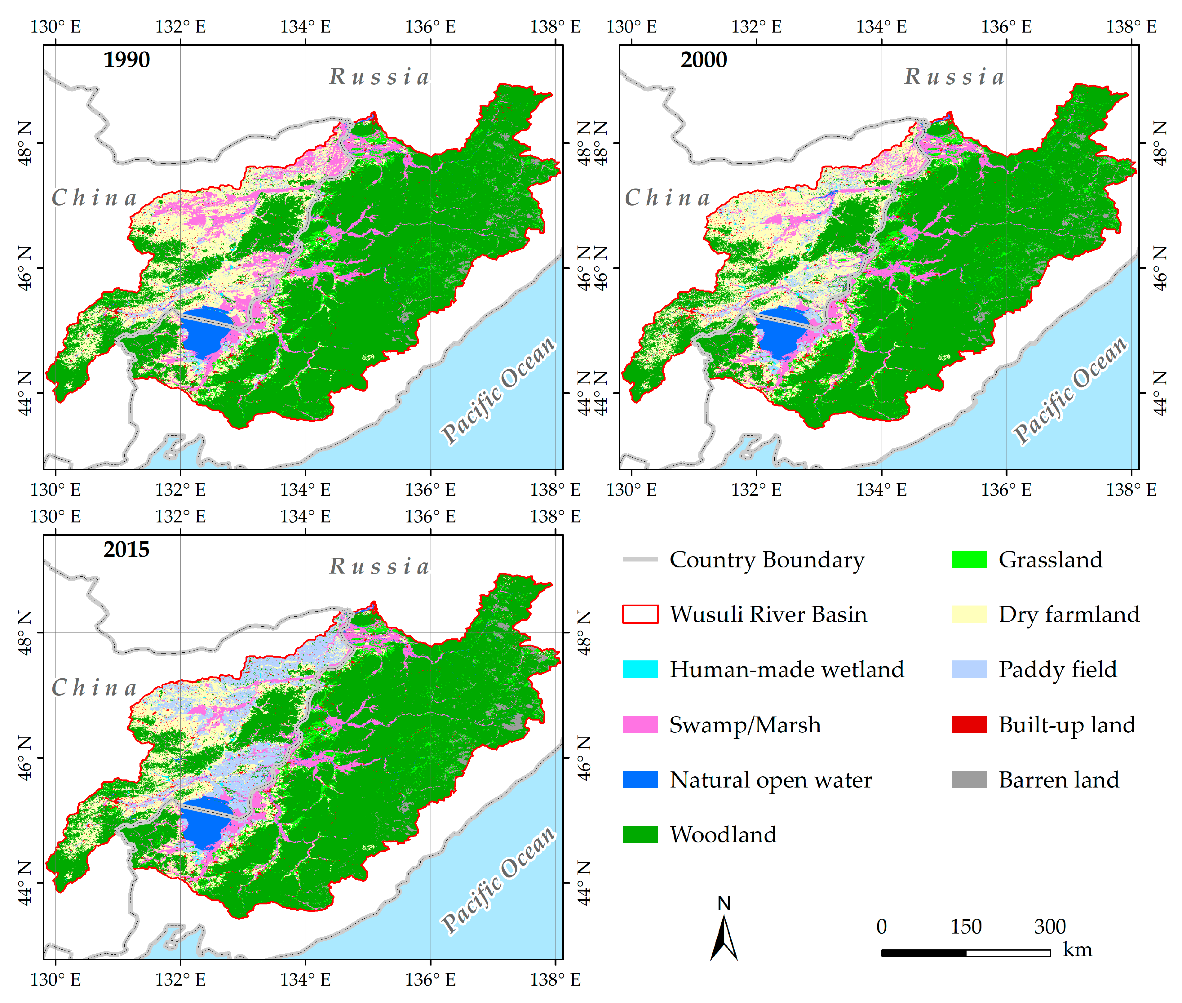
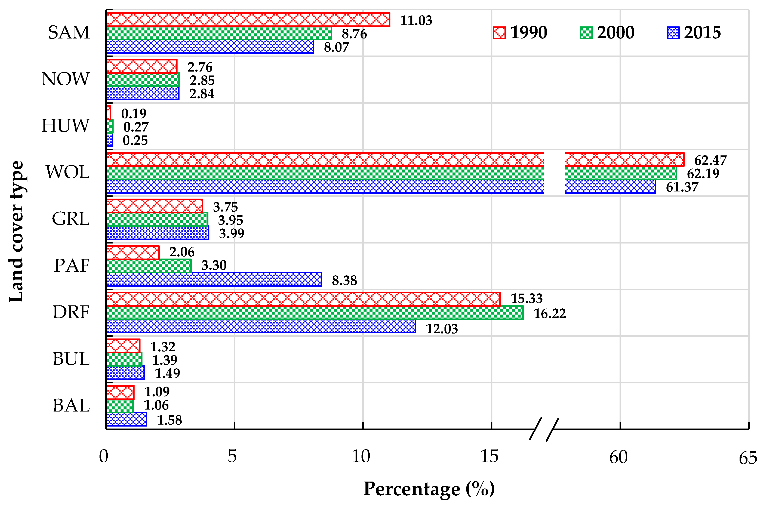
Figure 4 illustrates the spatio-temporal distribution of each land cover type in the study area from 1990 to 2015. The comparisons of the percentage of each land cover type are depicted in Figure 5.

Table 5. Annual land change area (ALCA) and annual land change rate (ALCR) of land cover types in the study area.

Landscape Category	Land Cover Type	China Portion						Russia Portion						Wusuli River Basin
		ALCR (%/y)			ALCA (km2/y)			ALCR (%/y)			ALCA (km2/y)			ALCR (%/y)			ALCA (km2/y)
		a	b	c	a	b	c	a	b	c	a	b	c	a	b	c	a	b	c
NAW	SAM	−4.49	−1.54	−2.30	−473.52	−89.45	−243.08	0.28	−0.01	0.11	30.71	−1.00	11.68	−2.06	−0.53	−1.08	−442.81	−90.45	−231.40
	NOW	0.54	−0.19	0.09	8.34	−3.13	1.46	0.26	0.04	0.13	9.98	1.52	4.91	0.34	−0.03	0.12	18.32	−1.61	6.36
HUW	HUW	5.41	−0.57	1.63	14.89	−2.43	4.49	0.98	−0.45	0.10	0.91	−0.46	0.09	4.30	−0.55	1.25	15.79	−2.89	4.58
WOL	WOL	−0.24	−0.11	−0.16	−46.37	−20.39	−30.78	−0.01	−0.08	−0.05	−9.12	−85.73	−55.09	−0.05	−0.09	−0.07	−55.48	−106.12	−85.87
GRL	GRL	−3.32	0.76	−1.02	−13.17	2.02	−4.06	0.74	0.05	0.33	51.58	3.38	22.66	0.52	0.07	0.25	38.41	5.40	18.61
CRL	PAF	8.62	12.22	17.10	249.98	660.14	496.08	−0.65	−0.01	−0.27	−7.23	−0.12	−2.97	6.05	10.24	12.28	242.75	660.02	493.11
	DRF	1.02	−2.09	−0.97	244.86	−551.57	−232.99	−1.17	0.12	−0.40	−69.71	6.30	−24.10	0.59	−1.72	−0.86	175.16	−545.27	−257.10
BUL	BUL	1.41	0.39	0.83	15.09	4.81	8.92	−0.03	0.56	0.32	−0.51	8.34	4.80	0.57	0.48	0.53	14.57	13.15	13.72
BAL	BAL	−2.70	−0.14	−1.14	−0.09	0.00	−0.04	−0.31	3.29	1.79	−6.49	67.77	38.06	−0.31	3.29	1.79	−6.58	67.77	38.03

Note: a, b, and c denote the stage of 1990–2000, 2000–2015 and 1990–2015, respectively.

shows the ALCA and ALCR of each land cover type. The results indicate that the natural wetlands (i.e., swamp/marsh and natural open water) of the Wusuli River Basin experienced a gradual decrease from 13.79% of the total area (26,892.99 km²) in 1990 to 10.91% of the total area (21,267.23 km²) in 2015, with an ALCA of −225.03 km²/y and an ALCR of −0.96%/y. Swamp/marsh decreased by 2.96% during the period 1990–2015, while the area of natural open water increased by 0.08%. From 1990 to 2000, swamp/marsh decreased dramatically, with a change rate of −42.81 km²/y. During 2000–2015, the reduction rate of the swamp/marsh area slowed over time, with an average rate of loss of 90.45 km²/y. Despite an annual reduction area of 85.87 km², woodland remained the dominant landscape type during the period 1990–2015, with the vast majority distributed in the Russian part of the catchment. Cropland expanded markedly with an average rate of gain of 236.01 km²/y, especially in 1990–2000 with an ALCR of 417.91 km²/y. Specifically, the distribution range of paddy field expanded from sporadic patches in 1990 to large-scale continuous areas in the Chinese section of the basin in 2015, and the area quadrupled. In contrast, dry farmland decreased overall from 15.33% of the total area in 1990 to 12.06% of the total area in 2015, mainly because of a rapid rate of decrease from 2000 to 2015 (ALCR was −545.27 km²/y). Human-made wetland, grassland, built-up land, and barren land had a slight areal increase during the period 1990–2015 with an ALCA of 4.58 km²/y, 18.61 km²/y, 13.72 km²/y, and 38.03 km²/y, respectively.

In terms of the different countries, in the Russian section of the Wusuli River Basin, woodland still accounted for more than three-fourths of the total landscape area from 1990 to 2015, despite an annual decline of 55.09 km². For croplands, both dry farmland and paddy field decreased by a small proportion. However, swamp/marsh and natural open water increased with an ALCA of 11.68 km²/y and 4.91 km²/y, respectively.

In the Chinese section, croplands were the largest land cover type from 1990 to 2015. Paddy field and dry farmland showed the opposite areal change trends. During 1990–2015, paddy fields increased more than five-fold in area, while dry farmlands decreased by 9.65%. The area of natural wetland almost halved, and their areal proportion reduced from 20.05% of the total area of the Chinese section to 10.04%, with an ALCA of 241.62 km²/y and an ALCR of −2.21%/y. The areal reduction of swamp/marsh accounted for the overwhelming majority of change in natural wetland with a loss rate of 243.08 km²/y, whereas no significant change occurred in the area of natural open water.

3.3. Conversion between Natural Wetland and Other Land Cover Types

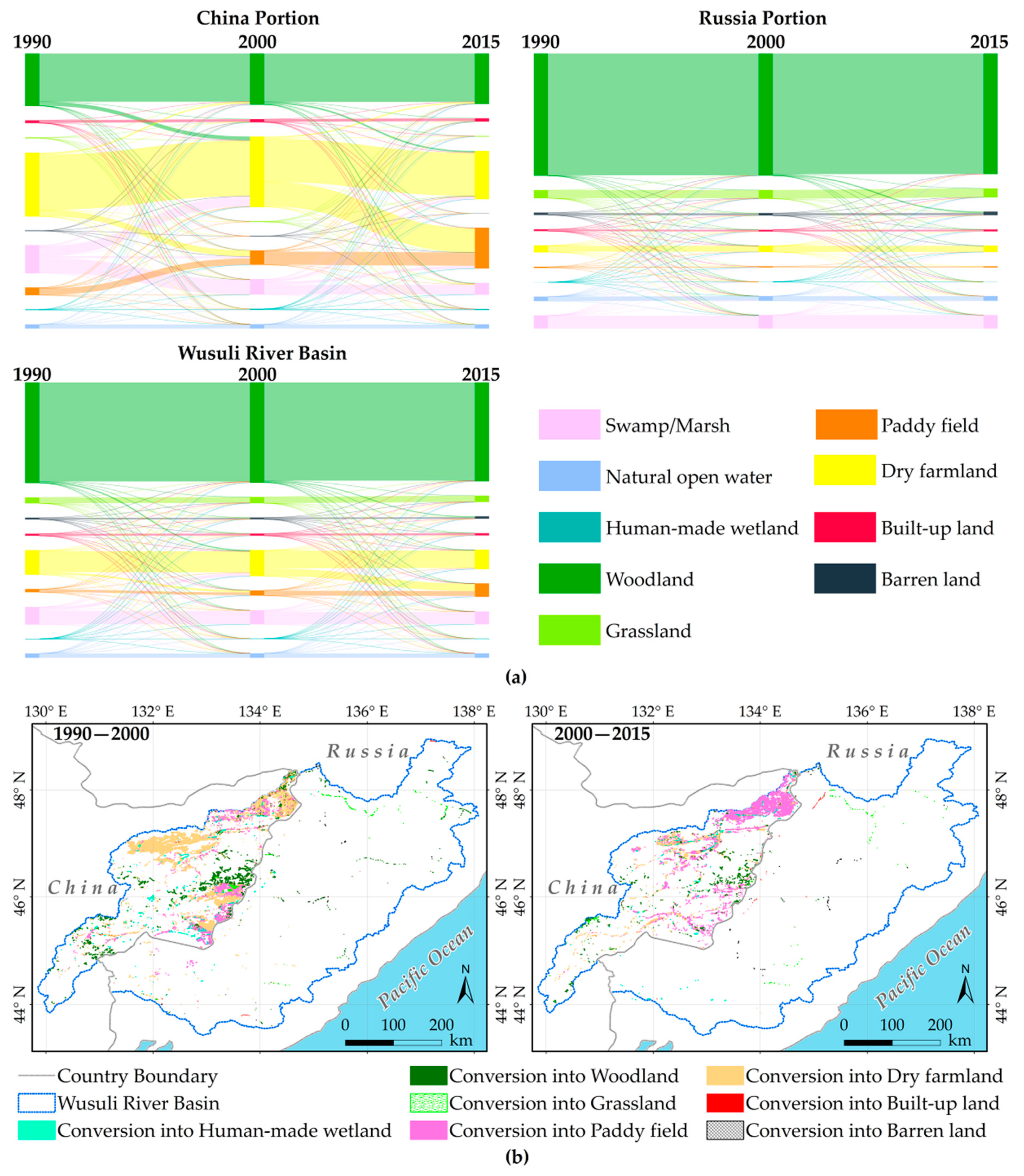
Figure 6 and

Table 6. Conversion comparison between natural wetlands and other land cover types in the study area.

Change Type	Conversion Area/km2
	China Part		Russia Part		Wusuli River Basin
	1990–2000	2000–2015	1990–2000	2000–2015	1990–2000	2000–2015
NAW→HUW	123.77	41.20	2.11	3.43	125.88	44.63
NAW→WOL	91.21	26.27	7.28	0.45	98.49	26.72
NAW→GRL	38.17	9.62	6.94	2.28	45.11	11.90
NAW→PAF	712.26	1043.13	11.97	0.00	724.23	1043.13
NAW→DRF	3720.86	897.74	29.89	0.12	3750.75	897.86
NAW→BUL	20.10	16.75	8.62	7.15	28.72	23.90
NAW→BAL	0.00	0.02	4.13	2.51	4.13	2.53
HUW→NAW	14.54	75.8	1.88	2.48	16.42	78.28
WOL→NAW	9.71	11.07	3.94	3.02	13.65	14.09
GRL→NAW	8.10	27.25	5.77	6.37	13.87	33.62
PAF→NAW	53.24	76.73	56.58	0.00	109.82	76.73
DRF→NAW	207.53	248.97	400.62	8.79	608.15	257.76
BUL→NAW	0.83	6.24	7.86	0.19	8.69	6.43
BAL→NAW	0.54	0.00	0.97	2.24	1.51	2.24

illustrate the conversions between natural wetland and other land cover types in terms of spatial distribution and area. Most of the natural wetland conversion occurred in the Chinese section of the Basin, while only a small proportion took place in the Russian section. Across the entire Wusuli River Basin, most of the natural wetland recession occurred from 1990 to 2000, attributed to the conversion of a large area to dry farmland and paddy field, which accounted for 78.51% and 15.16% of the natural wetland reduction in this stage, respectively. During the period 2000–2015, the percentage of conversion to dry farmland and paddy field was 43.78% and 50.87%, respectively. Between 1990 and 2000, 125.88 km² of natural wetlands were converted into human-made wetlands which reduced the area of natural wetlands. In terms of the transformation of other land cover types into natural wetlands, in both stages (1990–2000 and 2000–2015), the proportion of dry farmland converted into natural wetlands was the highest, accounting for 78.76% and 54.94%, respectively. Paddy field also contributed to the increase of natural wetlands, accounting for 14.22% and 16.36% of natural wetland area recovery in the stages 1990–2000 and 2000–2015, respectively. There was little reciprocal conversion among natural wetlands and woodland, grassland, built-up land or barren land during the period 1990–2015. These results suggest that the change in natural wetlands area can be attributed mainly to cropland reclamation and natural restoration from cropland.

For the Russian portion of the basin, the reclamation of natural wetlands covered a smaller area than their expansion during the two periods. Especially in the stage of 1990–2000, a total of 457.20 km² of natural wetlands were restored from cropland. Nevertheless, the reduced area of natural wetlands in the Chinese part of the basin was much larger than that of natural wetland restoration, suggesting a serious areal loss process.

3.4. Fragmentation and Improvement of Natural Wetland and Trend of Climate Change

Table 7. Landscape metrics comparison of the natural wetlands for the China portion and Russia portion of the Wusuli River Basin in1990, 2000 and 2015.

Year		NP	MPS	LPI	AWMSI	IJI
China part	1990	3387	357.18	16.81	57.07	54.58
	2000	3647	204.16	5.92	32.13	59.78
	2015	1384	437.66	4.67	27.05	68.58
Russia part	1990	2158	685.60	5.00	24.34	73.75
	2000	2236	679.88	5.24	24.55	73.38
	2015	2217	686.06	5.24	24.39	74.02

presents a comparison of the landscape metrics for natural wetlands in the Chinese and Russian sections of the Wusuli River Basin in 1990, 2000 and 2015. The landscape pattern of natural wetlands changed significantly in the Chinese part of the basin, while there was no significant change from 1990 to 2015 in the Russian part. During 1990–2015, despite a small increase in average patch area (MPS), the NP, LPI and AWMSI of natural wetlands decreased significantly in the Chinese portion, indicating that natural wetlands had undergone a loss and fragmentation process. In the Russian section, the NP, MPS, LPI and AWMSI of natural wetlands increased slightly, supporting the improvement which the natural wetlands had experienced in the Russian portion of the basin. There were more obvious changes in the IJI of natural wetlands in the Chinese part than in the Russian part of the basin, suggesting that the existence of natural wetland was subjected to more outside interference in the Chinese portion of the Wusuli River Basin.

Based on the Mann–Kendall test, there were no significant changes, at the 5% significant level, in the trend for the annual average temperature and annual precipitation in the Wusuli River Basin during the study period.

4. Discussion

4.1. Conservation and Threats of Anthropogenic Activities on Natural Wetland

Agriculture, considered as the primary foundation of a country’s development, is important for ensuring national security and people’s livelihoods [54]. In the past, reclaiming natural wetlands for croplands was seen as the best way to increase the cultivated land area to meet the need for grain production. Our results suggest that conversion into croplands was the primary contributor to natural wetland losses, especially in the Chinese section of the Wusuli River Basin (Table 5, Figure 6, and Table 6). Previous studies concerning the dynamics of natural wetlands in the Sanjiang Plain of China, have also shown that the loss and shrinkage of natural wetlands were generally caused by agricultural encroachment [55,56]. Indeed, there are a series of national and regional policies designed to stimulate natural wetland conversion into croplands in the Chinese part of the Wusuli River Basin [57]. In the 1990s, grain trade and crop cultivation were promoted by the establishment of a market-based economic system and comprehensive enforcement of a household responsibility system. The introduction of modern agricultural machinery also made agricultural encroachment more feasible [58,59]. To enhance grain security, the Heilongjiang province government has executed the project ‘Land Regulation and Reclamation’ since 2001. Owing to suitable geographical conditions, natural wetlands were seen as the most desirable land cover type for crop cultivation, especially in the Sanjiang Plain [60]. In 2004, the ‘Reform of Rural Taxes and Administrative Charges’ policy was first carried out in Heilongjiang Province [61], by which the agricultural tax was rescinded and subsides were granted to farmers according to their cultivated area. Because of the increase in farming profit in the context of the policy, significant areas of illegal cropland were developed in the Sanjiang Plain. During the past decade, a food security plan was launched in China aiming to increase an additional 50 million tons of grain production, which gave rise to a further wave of encroachment of croplands into natural wetlands [62].

As referenced by Mao et al. [54] and Lu et al. [63], agricultural plantation structures and hydraulic engineering construction are directly or indirectly responsible for the loss and degradation of natural wetland. From 1990 to 2015, the ratio of paddy fields to dry farmlands changed from 1:7.44 in 1990 to 1:1.44 in 2015, with a rapid expansion of paddy field (Figure 4 and Figure 5). On one hand, large areas of new expanded paddy field were converted from natural wetlands. Our findings showed that the area of natural wetlands converted into paddy field was 724.23 km² and 1043.13 km² in the stages 1990–2000 and 2000–2015, respectively (Figure 6 and Table 6). On the other hand, irrigation in paddy fields consumed a vast amount of groundwater and surface water, which affected hydrological processes and threatened the water replenishment source for natural wetland [64]. Furthermore, with the increase in human-made wetland, substantial water sources in natural wetland are extracted for irrigation to meet the water demand for cultivated land, which undoubtedly aggravates threats to the existence of natural wetland. A previous study stated that the implementation of the ‘Two Rivers and One Lake’ project in Heilongjiang province, which was aimed at redirecting surface water to complement farmland irrigation, resulted in insufficient water resources for natural wetlands [65]. This is consistent with our research.

Population change is another common underlying force in natural wetland dynamics. Over the period 1990–2015, the population of Heilongjiang province in China increased, with rapid growth in the stage 1990–2000 (Figure 7a). Greater demand for grain was triggered by increases in the population, which promoted crop cultivation and stimulated the alteration of natural wetlands [66]. In contrast, there was a declining population trend in the Primorsky Krai province of Russia (Figure 7b). Due to this depopulation trend, reclaimed lands were abandoned and gradually turned into natural wetlands. Nearly 466 km² of croplands reverted to natural wetlands in the Russian section of the Wusuli River Bain from 1990 to 2015 (Table 6).

As the eco-environmental values of natural wetlands have become more widely recognized, some ecological projects and conservation policies have been introduced to protect and restore them. Figure 8 illustrates pivotal ecological projects and conservation policies for natural wetland in China and Russia. It was found that the implementation of wetland protection measures in Russia occurred more than 60 years earlier than in China. Russia’s accession to the Ramsar Wetland Convention was 17 years earlier than that of China. Compared with China, earlier environmental protection laws, which included the conservation and rational use of natural wetlands, were promulgated in Russia. All of these differences allow Russia has more prerequisites for wetland protection than China. This probably explains why the natural wetlands in the Russian region of the Wusuli River Basin have gone through a process of gradual restoration and improvement. In the Chinese part of the basin, although natural wetlands have experienced a loss and fragmentation process, the rate of area reduction has decreased over time (Table 5). Since the “Chinese wetland protection action plan” was initiated in 2000, many feasible and effective wetland protection and restoration measures have been implemented successively, which play a substantial role in natural wetland restoration and conservation [67]. Our results show that, on the one hand, the area of natural wetland reduced by cropland encroachment in 2000–2015 was only 25.56% of that in 1990–2000, on the other hand, the area of natural wetland restored from croplands in 2000–2015 was 1.25 times that in 1990–2000 in Chinese part of Wusuli River Basin (Table 5). Therefore, it can be inferred that, due to the implementation of conservation policies and measures, the destruction and disturbance caused by human activities to natural wetland has been mitigated to some degree in the Chinese region of the basin.

As mentioned above, agricultural activity has been the most important reason for the loss of natural wetlands in Wusuli River Basin, especially in the Chinese portion. Different demographic change trends and wetland protection levels in China and Russia region have also had opposing effects on wetland existence and restoration.

4.2. Further Studies Required on Remaining Natural Wetlands

The approach used in this paper provides a practical option for understanding the driving factors for cross-boundary areas. Combining remotely sensed data with spatial analysis is a tractable, effective and labor-saving method to determine wetland dynamics and their driving forces in neighboring countries. However, several further studies also should be carried out for effective conservation and management remaining natural wetlands.

On the one hand, more precise wetland monitoring data are needed. The resolution of Landsat TM/OLI images limits the smallest unit of wetland and land cover identifiable from the satellite images to 0.09 ha. Therefore, the existence and loss of wetlands smaller than 0.09 ha would not be captured in the study though small wetland patches are more likely to be influenced by human activities and climate change [36,45].

On the other hand, it should be noted that, although no significant climate change was observed during the study periods, the impacts of climate change on natural wetland dynamics should receive on-going attention in the context of global warming. At present, such assessment is in the qualitative stage. Therefore, more objective and quantitative approaches should be developed, especially for a long-term sequential research project [68].

4.3. Conservation Suggestions of Cross-Boundary WPA in Wusuli River Basin

Comparative studies across administrative borders or along transects are a promising alternative for understanding the driving forces associated different national development strategies and eco-environmental policies on wetland effects, which can help develop effective conservation measures at a regional or even a global scale. The results from this study on the spatial and temporal change characteristics, and landscape pattern comparison of natural wetlands for the Chinese and Russian sections of the Wusuli River Basin (Figure 5 and Figure 6, and Table 7) can be taken as a guide for the formulation and implementation of conservation measure for wetlands in the Wusuli River Basin.

First, the Chinese and Russian governments should establish a bilateral cooperation mechanism to reinforce wetland ecosystem protection and maintain biodiversity. The managers, conservationists, and scientists of Russia and China should develop more feasible and effective plans to protect wetland ecosystems and to limit environmentally damaging human activities.

Second, regarding the Chinese government, more rigorous regulations and laws should be passed to prohibit people from converting natural wetlands into croplands [69,70]. For the areas in which natural wetlands have degraded, feasible wetland restoration projects should be implemented.

Third, establishing a wetland monitoring system is indispensable and allows for effective feedback on all aspects of wetlands. Moreover, adequate attention should be paid to the investigation and assessment of wetland biodiversity, which is related to the identification of key protected areas.

5. Conclusions

The monitoring and assessment for cross-boundary WPAs is essential to define the wetland dynamics as well as underpin knowledge-based conservation policies and funding decisions by bilateral government and managers. In the study, combining a rule-based object-oriented classification method, landscape metrics, spatial analysis and a Mann–Kendall test, we identified dynamic changes in natural wetlands and their influencing factors in the Wusuli River Basin from 1990 to 2015. Our results showed that the natural wetlands, as a whole, experienced a loss and fragmentation process, particularly in the Chinese section. Agricultural encroachment was the primary contributor to natural wetland degradation. In addition, differences in population trends and wetland conservation policies in the Chinese and Russian regions had differing effects on their natural wetland dynamics. The methods and results from this study can help our understanding of natural wetland changes and their driving forces in a cross-boundary study setting. These conclusions can be used as a guide for the bilateral government policies to effectively protect and manage natural wetlands.

References

1. Mitsch, W.J.; Gosselink, J.G. Wetlands, 2nd ed.; Van Nostrand Reinhold: New York, NY, USA, 1993; p. 722. [Google Scholar]
2. Kirwan, M.L.; Megonigal, J.P. Tidal wetland stability in the face of human impacts and sea-level rise. Nature 2013, 504, 53–60. [Google Scholar] [CrossRef]
3. Hu, S.J.; Niu, Z.G.; Chen, Y.F.; Li, L.F.; Zhang, H.Y. Global wetlands: Potential distribution, wetland loss, and status. Sci. Total Environ. 2017, 586, 319–327. [Google Scholar] [CrossRef]
4. Barbier, E.B.; Acreman, M.; Knowler, D. Economic Valuation of Wetlands: A Guide for Policy Makers and Planners, 1st ed.; Ramsar Convention Bureau: Gland, Switzerland, 1997; pp. 14–16. [Google Scholar]
5. Özesmi, S.L.; Bauer, M.E. Satellite remote sensing of wetlands. Wetl. Ecol. Manag. 2002, 10, 381–402. [Google Scholar] [CrossRef]
6. Wang, Z.M.; Zhang, B.; Zhang, S.Q.; Li, X.Y.; Liu, D.W.; Song, K.S.; Li, J.P.; Li, F.; Duan, H.T. Changes of land use and of ecosystem service values in Sanjiang Plain, Northeast China. Environ. Monit. Assess. 2006, 112, 69–91. [Google Scholar] [CrossRef] [PubMed]
7. Chaikumbung, M.; Doucouliagos, C.; Scarborough, H. The economic value of wetlands in developing countries: A meta-regression analysis. Ecol. Econ. 2016, 124, 164–174. [Google Scholar] [CrossRef]
8. Jia, M.M.; Wang, Z.M.; Zhang, Y.Z.; Mao, D.H.; Wang, C. Monitoring loss and recovery of mangrove forests during 42 years: The achievements of mangrove conservation in China. Int. J. Appl. Earth Obs. Geoinf. 2018, 73, 535–545. [Google Scholar] [CrossRef]
9. Mao, D.H.; He, X.Y.; Wang, Z.M.; Tian, Y.L.; Xiang, H.X.; Yu, H.; Man, W.D.; Jia, M.M.; Ren, C.Y.; Zheng, H.F. Diverse policies leading to contrasting impacts on land cover and ecosystem services in Northeast China. J. Clean. Prod. 2019, 240, 117961. [Google Scholar] [CrossRef]
10. Reis, V.; Hermoso, V.; Hamilton, S.K.; Ward, D.; Fluet-Chouinard, E.; Lehner, B.; Linke, S. A global assessment of inland wetland conservation status. Bioscience 2017, 67, 523–533. [Google Scholar] [CrossRef]
11. He, J.; Moffette, F.; Fournier, R.; Revéret, J.P.; Théau, J.; Dupras, J.; Boyer, J.P.; Varin, M. Meta-analysis for the transfer of economic benefits of ecosystem services provided by wetlands within two watersheds in Quebec, Canada. Wetl. Ecol. Manag. 2015, 23, 707–725. [Google Scholar] [CrossRef]
12. Gerakis, P.A. Conservation and management of Greek wetlands. In Proceedings of the Greek Wetlands Workshop, Thessaloniki, Greece, 17–21 April 1989; IUCN: Gland, Switzerland, 1992; p. 493. [Google Scholar]
13. Taft, O.W.; Haig, S.M.; Kiilsgaard, C. Use of radar remote sensing (RADARSAT) to map winter wetland habitat for shorebirds in an agricultural landscape. Environ. Manag. 2004, 33, 750–763. [Google Scholar] [CrossRef]
14. OECD/IUCN. Guidelines for Aid Agencies for Improved Conservation and Sustainable Use of Tropical and Sub-Tropical Wetlands, 1st ed.; OECD: Paris, France, 1996; pp. 7–8. [Google Scholar]
15. Rebelo, L.M.; Finlayson, C.M.; Nagabhatla, N. Remote sensing and GIS for wetland inventory, mapping and change analysis. J. Environ. Manag. 2009, 90, 2144–2153. [Google Scholar] [CrossRef] [PubMed]
16. Amler, E.; Schmidt, M.; Menz, G. Definitions and mapping of east African wetlands: A review. Remote Sens. 2015, 7, 5256–5282. [Google Scholar] [CrossRef]
17. Van Asselen, S.; Verburg, P.H.; Vermaat, J.E.; Janse, J.H. Drivers of wetland conversion: A global meta-analysis. PLoS ONE 2013, 8, e81292. [Google Scholar] [CrossRef] [PubMed]
18. Davidson, N.C. How much wetland has the world lost? Long-term and recent trends in global wetland area. Mar. Freshw. Res. 2014, 65, 934–941. [Google Scholar] [CrossRef]
19. Baker, C.; Lawrence, R.; Montagne, C.; Patten, D. Mapping wetlands and riparian areas using Landsat ETM+ imagery and decision-tree-based models. Wetlands 2006, 26, 465–474. [Google Scholar] [CrossRef]
20. Sica, Y.V.; Quintana, R.D.; Radeloff, V.C.; Gavier-Pizarro, G.I. Wetland loss due to land use change in the Lower Paraná River Delta, Argentina. Sci. Total Environ. 2016, 568, 967–978. [Google Scholar] [CrossRef]
21. Chen, L.F.; Jin, Z.Y.; Michishita, R.; Cai, J.; Yue, T.X.; Chen, B.; Xu, B. Dynamic monitoring of wetland cover changes using time-series remote sensing imagery. Ecol. Inf. 2014, 24, 17–26. [Google Scholar] [CrossRef]
22. Gottgens, J.F.; Swartz, B.P.; Kroll, R.W.; Eboch, M. Long-term GIS-based records of habitat changes in a Lake Erie coastal marsh. Wetl. Ecol. Manag. 1998, 6, 5–17. [Google Scholar] [CrossRef]
23. Garg, J.K. Wetland assessment, monitoring and management in India using geospatial techniques. J. Environ. Manag. 2015, 148, 112–123. [Google Scholar] [CrossRef]
24. Bürgi, M.; Hersperger, A.M.; Schneeberger, N. Driving forces of landscape change-current and new directions. Landsc. Ecol. 2005, 19, 857–868. [Google Scholar] [CrossRef]
25. Tuvi, E.L.; Vellak, A.; Reier, Ü.; Szava-kovats, R.; Pärtel, M. Establishment of protected areas in different ecoregions, ecosystems, and diversity hotspots under successive political systems. Biol. Conserv. 2011, 5, 1726–1732. [Google Scholar] [CrossRef]
26. Caddell, R. Nature Conservation in Estonia: From Soviet Union to European Union. J. Balt. Stud. 2009, 3, 307–332. [Google Scholar] [CrossRef]
27. Szantoi, Z.; Brink, A.; Buchanan, G.; Bastin, L.; Lupi, A.; Simonetti, D.; Mayaux, P.; Peedell, S.; Davy, J. A simple remote sensing based information system for monitoring sites of conservation importance. Remote Sens. Ecol. Conserv. 2016, 2, 16–24. [Google Scholar] [CrossRef]
28. Wang, X.P.; Guo, K. Basic implication of transboundary reserve and park for peace and their application. Guihaia 2004, 3, 220–223. [Google Scholar]
29. Zbicz, D.C. The “nature” of transboundary cooperation. Environ. Sci. Policy Sustain. Dev. 1999, 3, 15–16. [Google Scholar] [CrossRef]
30. Shi, L.Y.; Li, D.; Chen, L.; Zhao, Y. Transboundary protected areas as a means to biodiversity conservation. Acta Ecol. Sin. 2012, 21, 6892–6900. [Google Scholar]
31. Dahl, T.E.; Watmough, M.D. Current approaches to wetland status and trends monitoring in prairie Canada and the continental United States of America. Can. J. Remote Sens. 2007, 33, S17–S27. [Google Scholar] [CrossRef]
32. Xu, W.H.; Pimm, S.L.; Du, A.; Su, Y.; Fan, X.Y.; An, L.; Liu, J.G.; Ouyang, Z.Y. Transforming protected area management in China. Trends Ecol. Evol. 2019, 34, 762–766. [Google Scholar] [CrossRef]
33. Fent, A.; Bardou, R.; Carney, J.; Cavanaugh, K. Transborder political ecology of mangroves in Senegal and The Gambia. Glob. Environ. Chang. 2019, 54, 214–226. [Google Scholar] [CrossRef]
34. ESRI Inc. ArcGIS Desktop: Release 10; Environmental Systems Research Institute: Redlands, CA, USA, 2011. [Google Scholar]
35. Liu, H.Y.; Lu, X.G.; Wang, C.K. Study on the sustainable development of wetland resources in the Ussuri/Wusuli River basin. Chin. Geogr. Sci. 2000, 10, 270–275. [Google Scholar] [CrossRef]
36. Zhang, J.Y.; Ma, K.M.; Fu, B.J. Wetland loss under the impact of agricultural development in the Sanjiang Plain, NE China. Environ. Monit. Assess. 2010, 166, 139–148. [Google Scholar] [CrossRef] [PubMed]
37. EXELIS Inc. ENVI®5.1 Fast Line-of-Sight Atmospheric Analysis of Hypercubes (FLAASH); EXELIS Inc.: Boulder, CO, USA, 2013. [Google Scholar]
38. Lu, C.Y.; Gu, W.; Dai, A.H.; Wei, H.Y. Assessing habitat suitability based on geographic information system (GIS) and fuzzy: A case study of Schisandra sphenanthera Rehd. et Wils. in Qinling Mountains, China. Ecol. Model. 2012, 242, 105–115. [Google Scholar] [CrossRef]
39. Xia, Q.; Qin, C.Z.; Li, H.; Huang, C.; Su, F.Z. Mapping mangrove forests based on multi-tidal high-resolution satellite imagery. Remote Sens. 2018, 10, 1343. [Google Scholar] [CrossRef]
40. Baatz, M.; Schäpe, A. Multiresolution segmentation: An optimization approach for high quality multi-scale image segmentation. In Proceedings of the 12th Angewandte Geographische Informations Verarbeitung, Heidelberg, Germany, 12 December 2000. [Google Scholar]
41. Baatz, M.; Schäpe, A. Multiresolution segmentation: An optimization approach for high quality multi-scale imagesegmentation. Angew. Geogr. Inf. 2000, 12, 12–23. [Google Scholar]
42. Liu, M.Y.; Li, H.Y.; Li, L.; Man, W.D.; Jia, M.M.; Wang, Z.M.; Lu, C.Y. Monitoring the invasion of Spartina alterniflora using multi-source high-resolution imagery in the Zhangjiang Estuary, China. Remote Sens. 2017, 9, 539. [Google Scholar] [CrossRef]
43. Conchedda, G.; Durieux, L.; Mayaux, P. An object-based method for mapping and change analysis in mangrove ecosystems. ISPS J. Photogramm. 2008, 63, 578–589. [Google Scholar] [CrossRef]
44. Definiens Imaging. In eCognition Developer Software: 8.7.1. Reference Book; Trimble GmbH: Raunheim, Germany, 2012.
45. Lu, C.Y.; Liu, J.F.; Jia, M.M.; Liu, M.Y.; Man, W.D.; Fu, W.W.; Zhong, L.X.; Lin, X.Q.; Su, Y.; Gao, Y.B. Dynamic analysis of mangrove forests based on an optimal segmentation scale model and multi-seasonal images in Quanzhou Bay, China. Remote Sens. 2018, 10, 2020. [Google Scholar] [CrossRef]
46. Blaschke, T. Object based image analysis for remote sensing. ISPRS J. Photogram. 2010, 65, 2–16. [Google Scholar] [CrossRef] [Green Version]
47. Adam, E.; Mutanga, O.; Rugege, D. Multispectral and hyperspectral remote sensing for identification and mapping of wetland vegetation: A review. Wetl. Ecol. Manag. 2010, 18, 281–296. [Google Scholar] [CrossRef]
48. Zhou, X.R.; Liu, J.; Liu, S.G.; Cao, L.; Zhou, Q.M.; Huang, H.W. A GIHS-based spectral preservation fusion method for remote sensing images using edge restored spectral modulation. ISPRS J. Photogram. 2014, 88, 16–27. [Google Scholar] [CrossRef]
49. Duque, J.C.; Patino, J.E.; Ruiz, L.A.; Pardo-Pascual, J.E. Measuring intra-urban poverty using land cover and texture metrics derived from remote sensing data. Landsc. Urban Plan. 2015, 135, 11–21. [Google Scholar] [CrossRef]
50. Cuba, N. Research note: Sankey diagrams for visualizing land cover dynamics. Landsc. Urban Plan. 2015, 139, 163–167. [Google Scholar] [CrossRef]
51. Fragstats Help Version 4.2. Available online: http://www.umass.edu/landeco/research/fragstats/documents/fragstats.help.4.2.pdf (accessed on 21 April 2015).
52. Wang, H.J.; Chen, Y.N.; Chen, Z.S.; Li, W.H. Changes in annual and seasonal temperature extremes in the arid region of china, 1960–2010. Nat. Hazards 2013, 65, 1913–1930. [Google Scholar] [CrossRef]
53. McGarigal, K.; Ene, E. FRAGSTATS v4.2: A Spatial Pattern Analysis Program for Categorical Maps; University of Massachusetts: Amherst, MA, USA, 2012. [Google Scholar]
54. Mao, D.H.; Luo, L.; Wang, Z.M.; Wilson, M.C.; Zeng, Y.; Wu, B.F.; Wu, J.G. Conversions between natural wetlands and farmland in China: A multiscale geospatial analysis. Sci. Total Environ. 2018, 634, 550–560. [Google Scholar] [CrossRef] [PubMed]
55. Song, K.S.; Wang, Z.M.; Li, L.; Tedesco, L.; Li, F.; Jin, C.; Du, J. Wetlands shrinkage, fragmentation and their links to agriculture in the Muleng–Xingkai Plain, China. J. Environ. Manag. 2012, 111, 120–132. [Google Scholar] [CrossRef] [PubMed]
56. Wang, Z.M.; Song, K.S.; Ma, W.H.; Ren, C.Y.; Zhang, B.; Liu, D.W.; Chen, J.M.; Song, C.C. Loss and fragmentation of marshes in the Sanjiang Plain, Northeast China, 1954–2005. Wetlands 2011, 31, 945–954. [Google Scholar] [CrossRef]
57. Wang, Z.M.; Wu, J.G.; Madden, M.; Mao, D.H. China’s wetlands: Conservation plans and policy impacts. AMBIO 2012, 41, 782–786. [Google Scholar] [CrossRef]
58. Wang, G.G.; Liu, Y.S.; Li, Y.R.; Chen, Y.F. Dynamic trends and driving forces of land use intensification of cultivated land in China. J. Geogr. Sci. 2015, 25, 45–57. [Google Scholar] [CrossRef]
59. Song, K.S.; Wang, Z.M.; Du, J.; Liu, L.; Zeng, L.H.; Ren, C.Y. Wetland degradation: Its driving forces and environmental impacts in the Sanjiang Plain, China. Environ. Manag. 2014, 54, 255–271. [Google Scholar] [CrossRef]
60. Wang, H.X.; Zhang, M.H.; Cai, Y. Problems, challenges, and strategic options of grain security in China. Adv. Agron. 2009, 103, 101–147. [Google Scholar]
61. Tao, R.; Qin, P. How has rural tax reform affected farmers and local governance in China? China World Econ. 2007, 15, 19–32. [Google Scholar] [CrossRef]
62. Man, W.D.; Yu, H.; Li, L.; Liu, M.Y.; Mao, D.H.; Ren, C.Y.; Wang, Z.M.; Jia, M.M.; Miao, Z.H.; Lu, C.Y.; et al. Spatial expansion and soil organic carbon storage changes of croplands in the Sanjiang plain, China. Sustainability 2017, 9, 563. [Google Scholar] [CrossRef]
63. Lu, C.Y.; Wang, Z.M.; Li, L.; Wu, P.Z.; Mao, D.H.; Jia, M.M.; Dong, Z.Y. Assessing the conservation effectiveness of wetland protected areas in Northeast China. Wetl. Ecol. Manag. 2016, 24, 381–398. [Google Scholar] [CrossRef]
64. Chen, H.J.; Wang, G.P.; Lu, X.G.; Jiang, M.; Mendelssohn, I.A. Balancing the needs of China’s wetland conservation and rice production. Environ. Sci. Technol. 2015, 49, 6385–6393. [Google Scholar] [CrossRef] [PubMed]
65. Man, W.D.; Wang, Z.M.; Liu, M.Y.; Lu, C.Y.; Jia, M.M.; Mao, D.H.; Ren, C.Y. Spatio-temporal dynamics analysis of cropland in Northeast China during 1990–2013 based on remote sensing. Trans. Chin. Soc. Agric. Eng. 2016, 32, 1–10. (In Chinese) [Google Scholar]
66. Grumbine, R.E. Assessing environmental security in China. Front. Ecol. Environ. 2014, 12, 403–411. [Google Scholar] [CrossRef]
67. Mao, D.H.; Wang, Z.M.; Wu, J.G.; Wu, B.F.; Zeng, Y.; Song, K.S.; Yi, K.P.; Luo, L. China’s wetlands loss to urban expansion. Land Degrad. Dev. 2018, 29, 2644–2657. [Google Scholar] [CrossRef]
68. Junk, W.J.; An, S.Q.; Finlayson, C.M.; Gopal, B.; Květ, J.; Mitchell, S.A.; Mitsch, W.J.; Robarts, R.D. Current state of knowledge regarding the world’s wetlands and their future under global climate change: A synthesis. Aquat. Sci. 2013, 75, 151–167. [Google Scholar] [CrossRef]
69. Stem, C.; Margoluis, R.; Salafsky, N.; Brown, M. Monitoring and evaluation in conservation: A review of trends and approaches. Conserv. Biol. 2005, 19, 295–309. [Google Scholar] [CrossRef]
70. Knight, A.T.; Driver, A.; Cowling, R.M.; Maze, K.; Desmet, P.G.; Lombard, A.T.; Rouget, M.; Botha, M.A.; Boshoff, A.F.; Castley, G.J.; et al. Designing systematic conservation assessments that promote effective implementation: Best practice from South Africa. Conserv. Biol. 2006, 20, 739–750. [Google Scholar] [CrossRef]
Figure 1. Location of the Wusuli River Basin.
Remotesensing 11 02581 g001
Figure 2. The location of meteorological stations, field survey points and ground reference data sites.
Remotesensing 11 02581 g002
Figure 3. Rules for the land cove classification of the Wusuli River Basin (α, β, γ, δ, ε, and ζ, represent the selected classification parameters and each of them could vary for different images (Landsat TM/OLI: Landsat Thematic Mapper/Operational Land Imager; NDVI: Normalized difference vegetation index; LSWI: Land surface water index; SI: Shape index; SWIR1: Short wave infrared band1, corresponding to Landsat TM Band 5 and Landsat OLI Band 6, respectively; NIR: Near infrared band, corresponding to Landsat TM Band 4 and Landsat OLI Band 5, respectively; Red: Red band, corresponding to Landsat TM Band 3 and Landsat OLI Band 4, respectively; Unwater area: Land areas covered without water, including built-up area, barren land, woodland, grassland, swamp/marsh, dry farmland and paddy field).
Remotesensing 11 02581 g003
Figure 4. Land cover maps of the Wusuli River Basin in 1990, 2000 and 2015.
Remotesensing 11 02581 g004
Figure 5. Area percentage of each land cover type for the Wusuli River Basin in 1990, 2000 and 2015.
Remotesensing 11 02581 g005
Figure 6. Dynamic conversion comparisons between natural wetlands and other land cover types. (a) Sankey diagram for comparison of total land cover dynamics from 1990 to 2015; (b) Spatial distribution of conversion between natural wetlands and other land cover types in two stages, 1990–2000 and 2000–2015.
Remotesensing 11 02581 g006
Figure 7. Population change for the Heilongjiang province of China (a) and the Primorsky Krai province of Russia (b) from 1990 to 2015.
Remotesensing 11 02581 g007
Figure 8. Comparison of ecological projects and conservation policies between China and Russia in Wusuli River Basin.
Remotesensing 11 02581 g008