Bistatic Landmine and IED Detection Combining Vehicle and Drone Mounted GPR Sensors

 , , and
Abstract
:
1. Introduction
2. Methodology
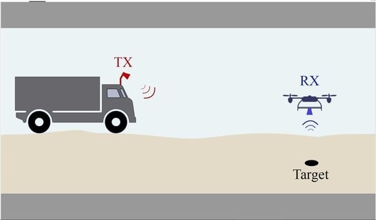
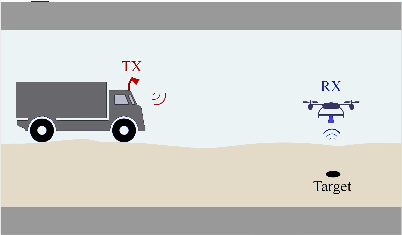
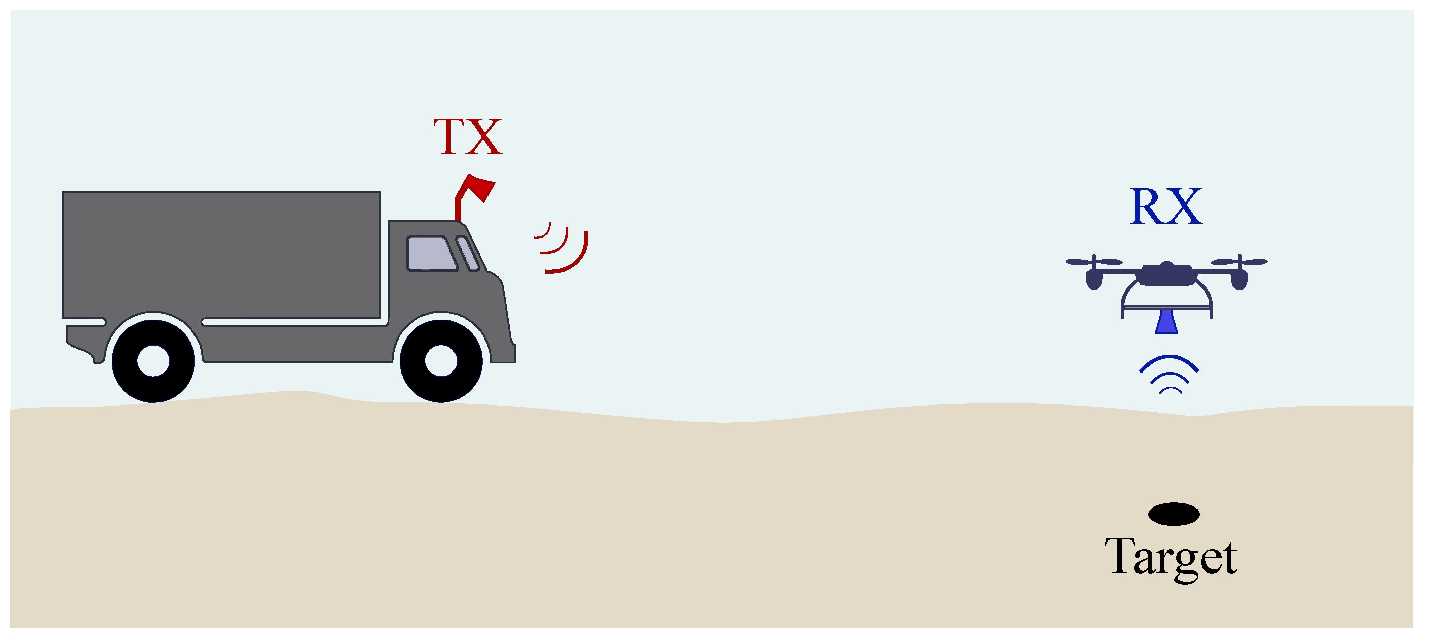
2.1. Scenario
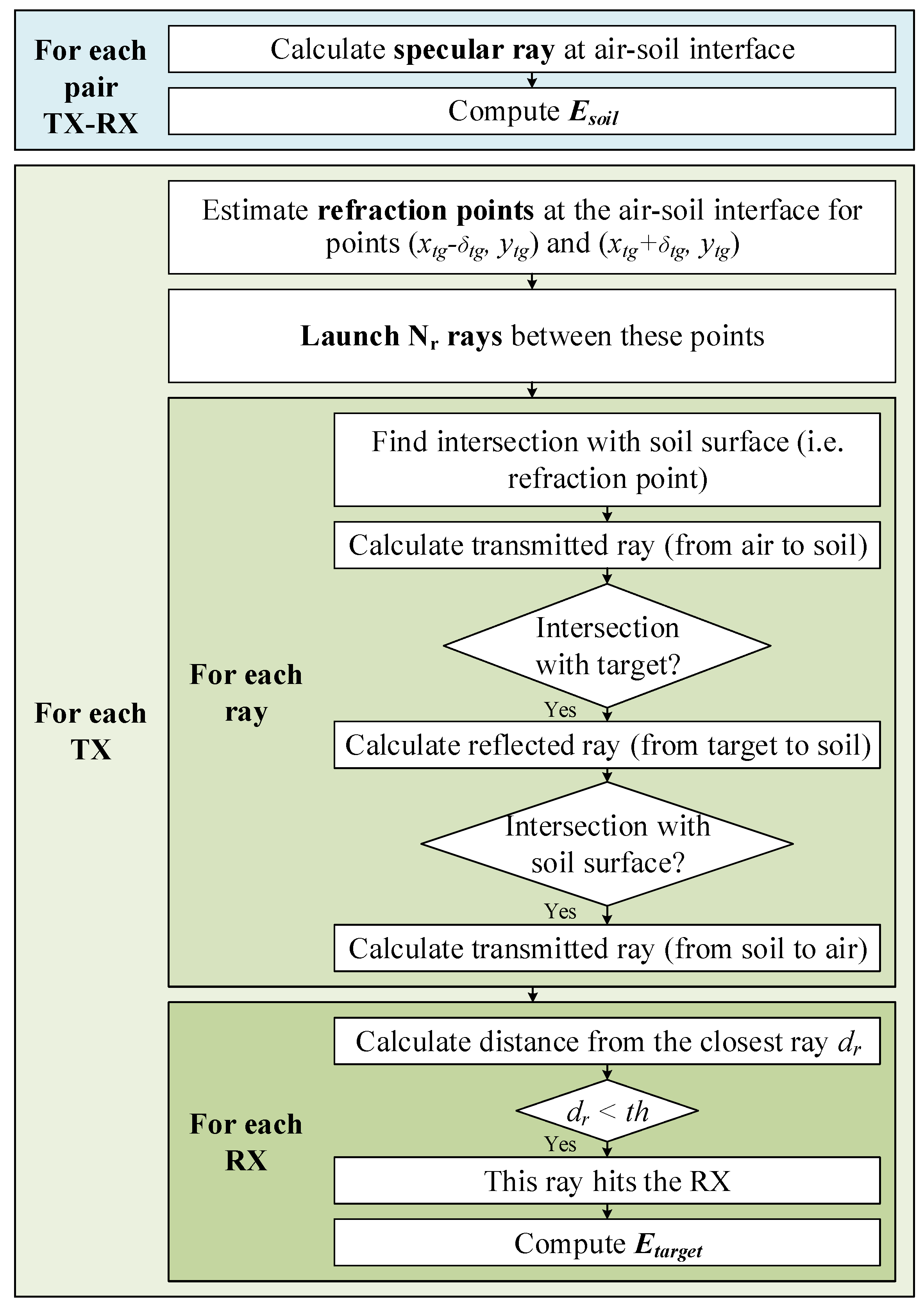
2.2. Ray-Tracing
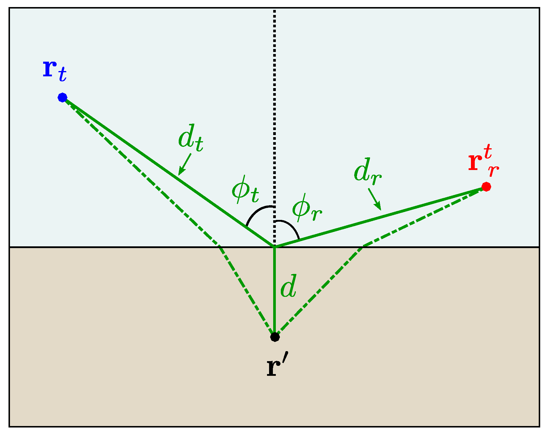
2.2.1. Field Computation
2.2.2. Implementation
2.3. FDFD
2.4. Inversion
3. Results
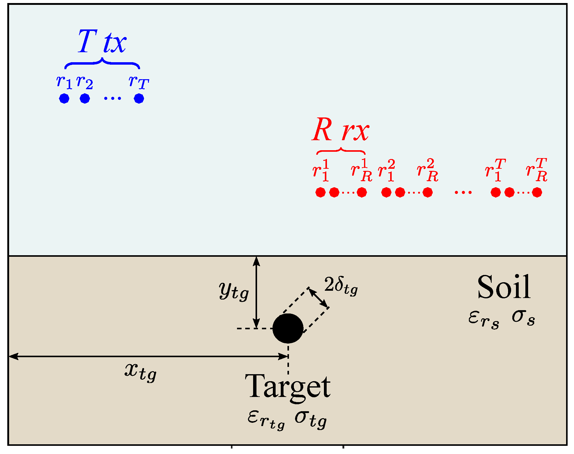
3.1. Scenario Configuration
- Multimonostatic, where the TX–RX (drone mounted transceiver) is placed at 65 different positions between down-track positions m and m at m height. The angle of incidence is (i.e., the antennas are aligned perpendicular to the soil surface, with main beam pointing straight down).
- Multistatic, where the TX is placed at a fixed position (on a vehicle, at down-track position m and height m) with main beam pointing at an angle of incidence of with the nominal ground surface, and the drone-mounted RX is looking downward and is moved to the same positions as in the multimonostatic case.
- Multibistatic, where the vehicle-mounted TX is placed at m height and is moved between down-track positions m and m and the drone-mounted RX is moved between the same positions as in the multimonostatic case. Thus, both TX and RX are moved coherently. The angles of incidence are for the TX and for the RX.
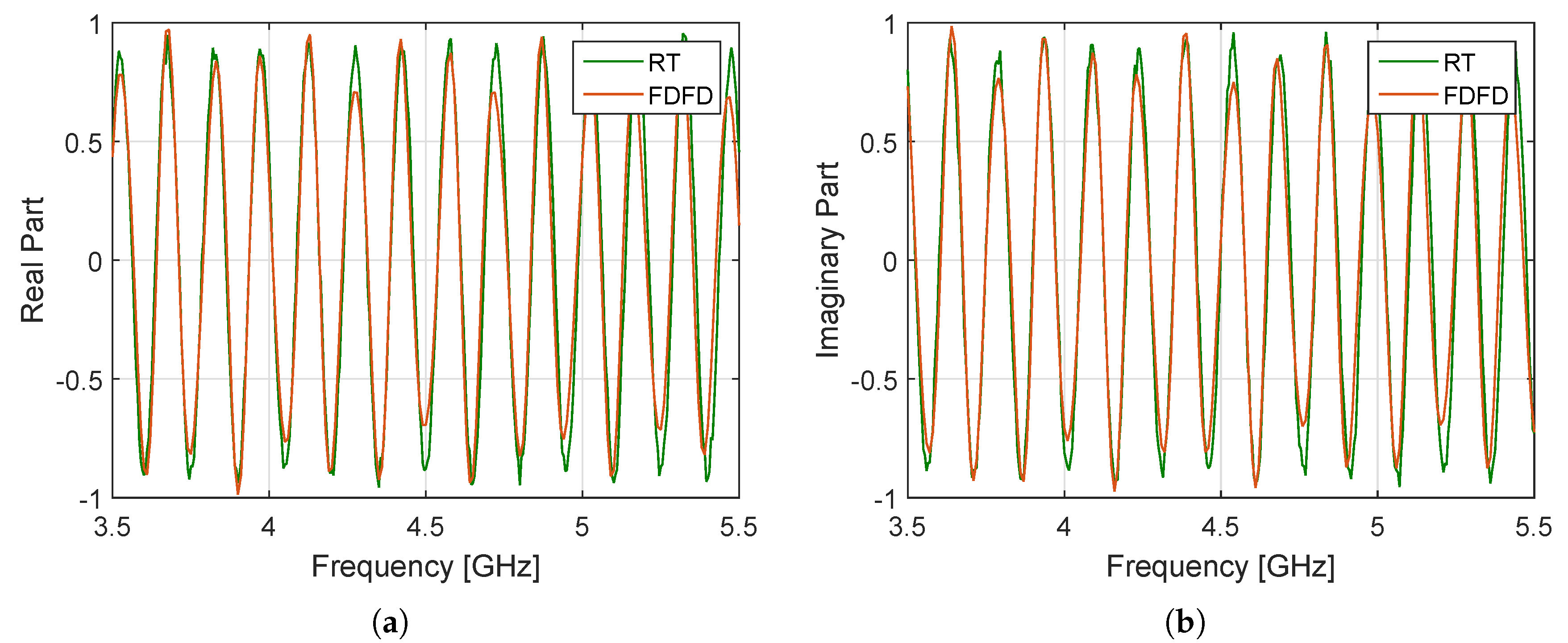
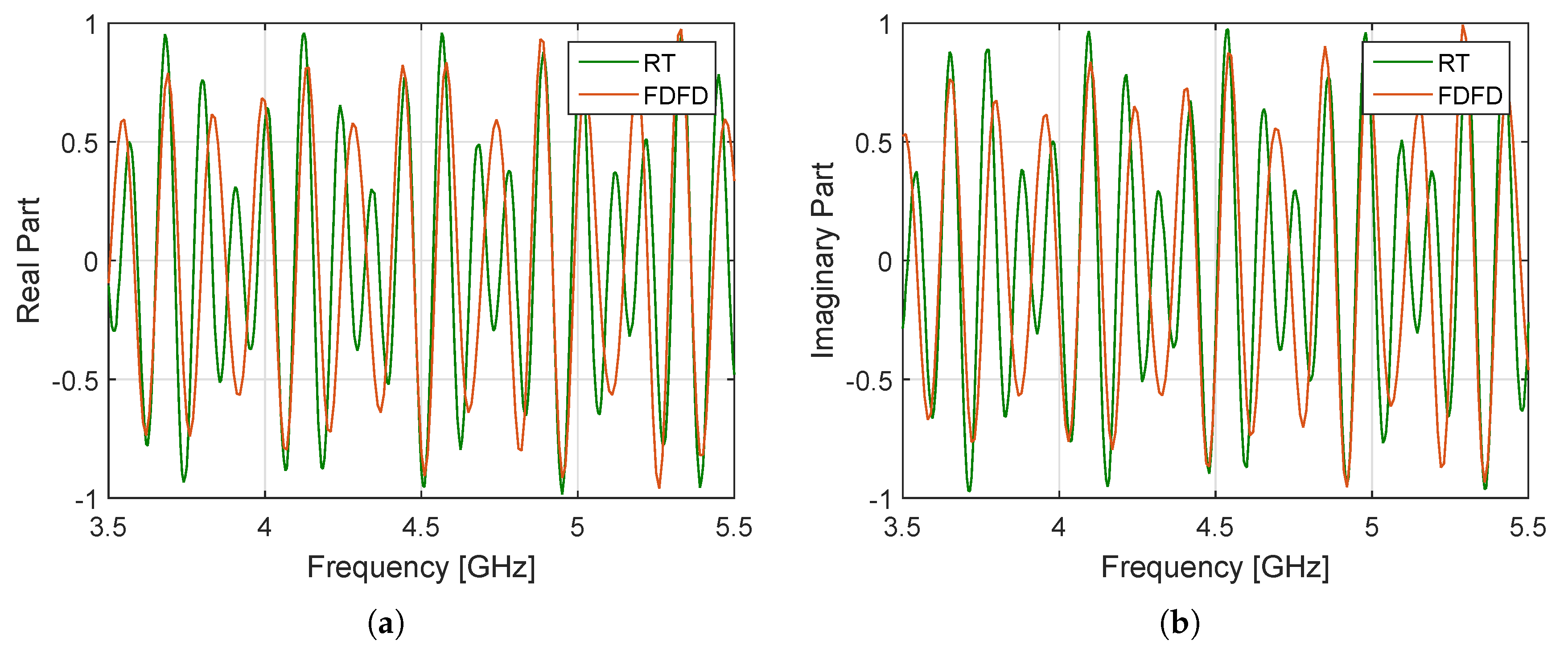
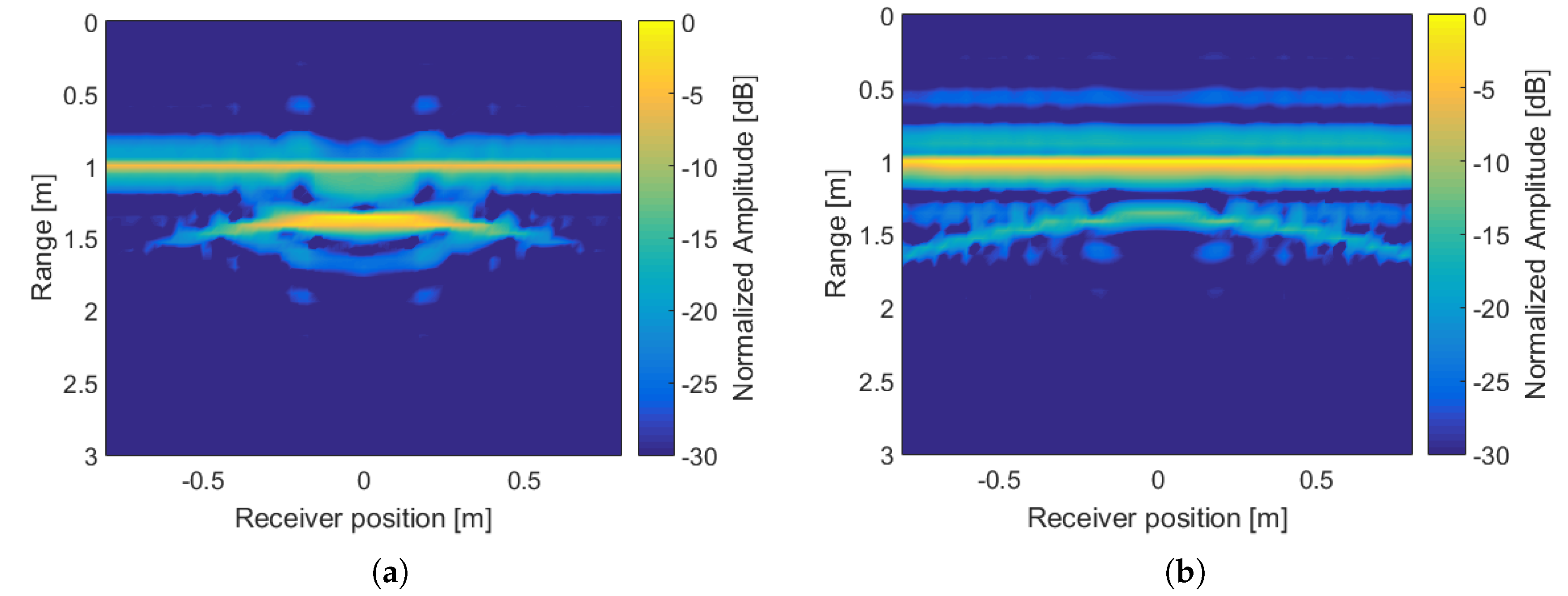
3.2. Initial Comparison: Scattered Field and B-Scan
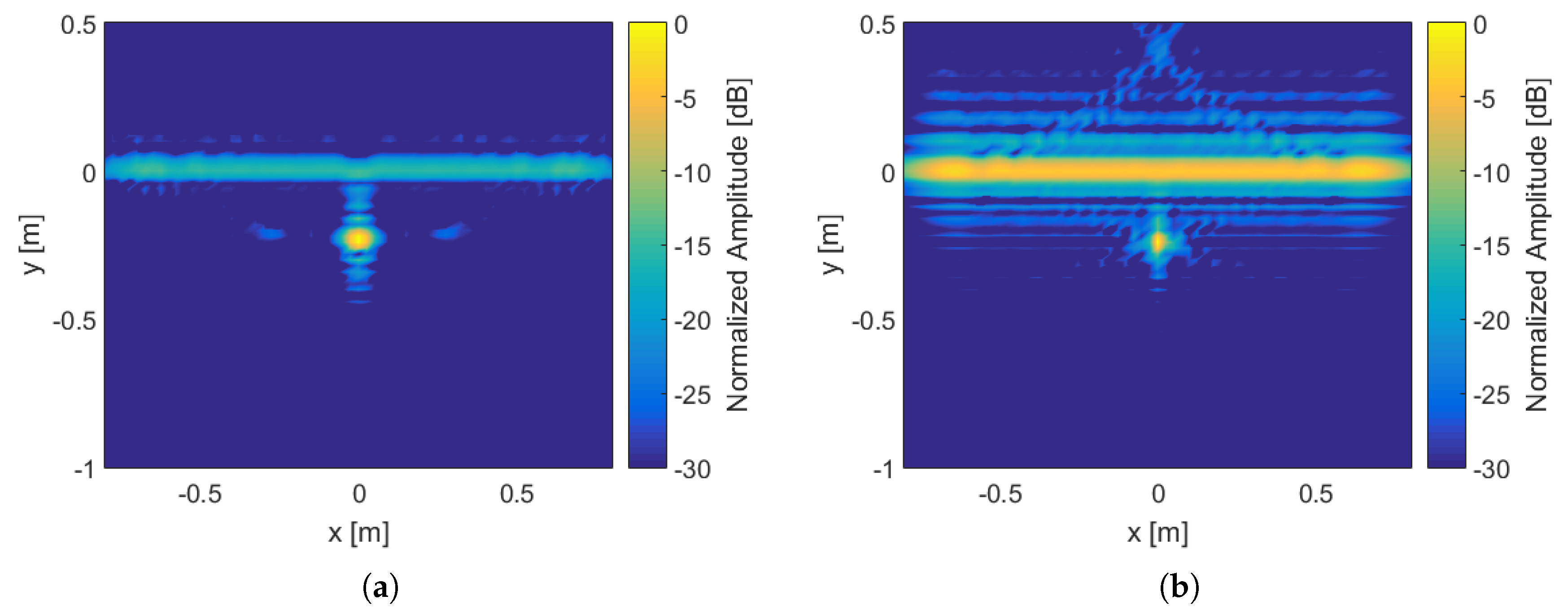
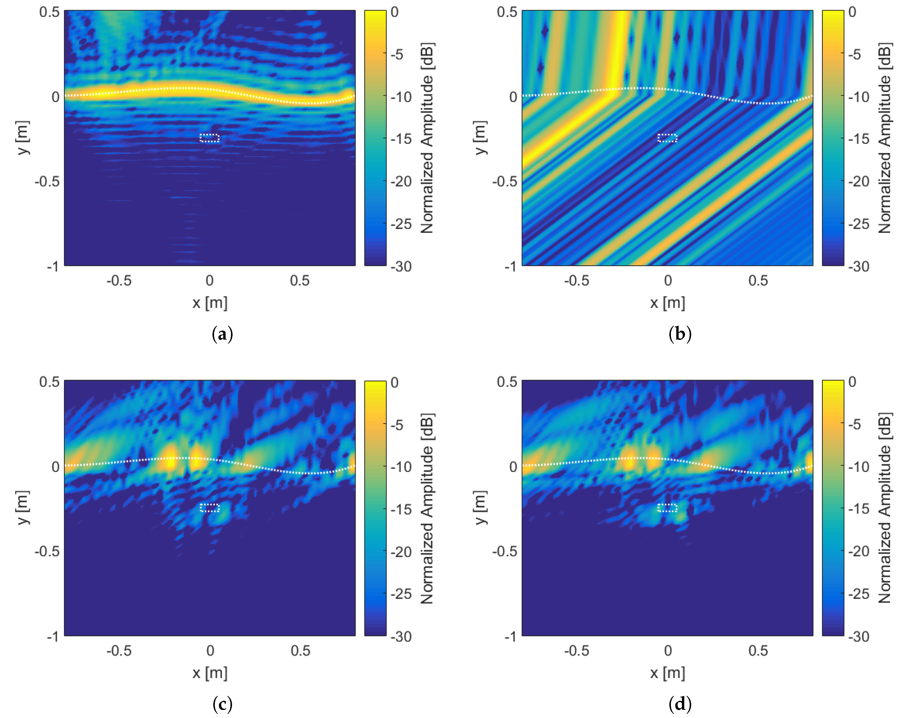
3.3. SAR Image Comparison
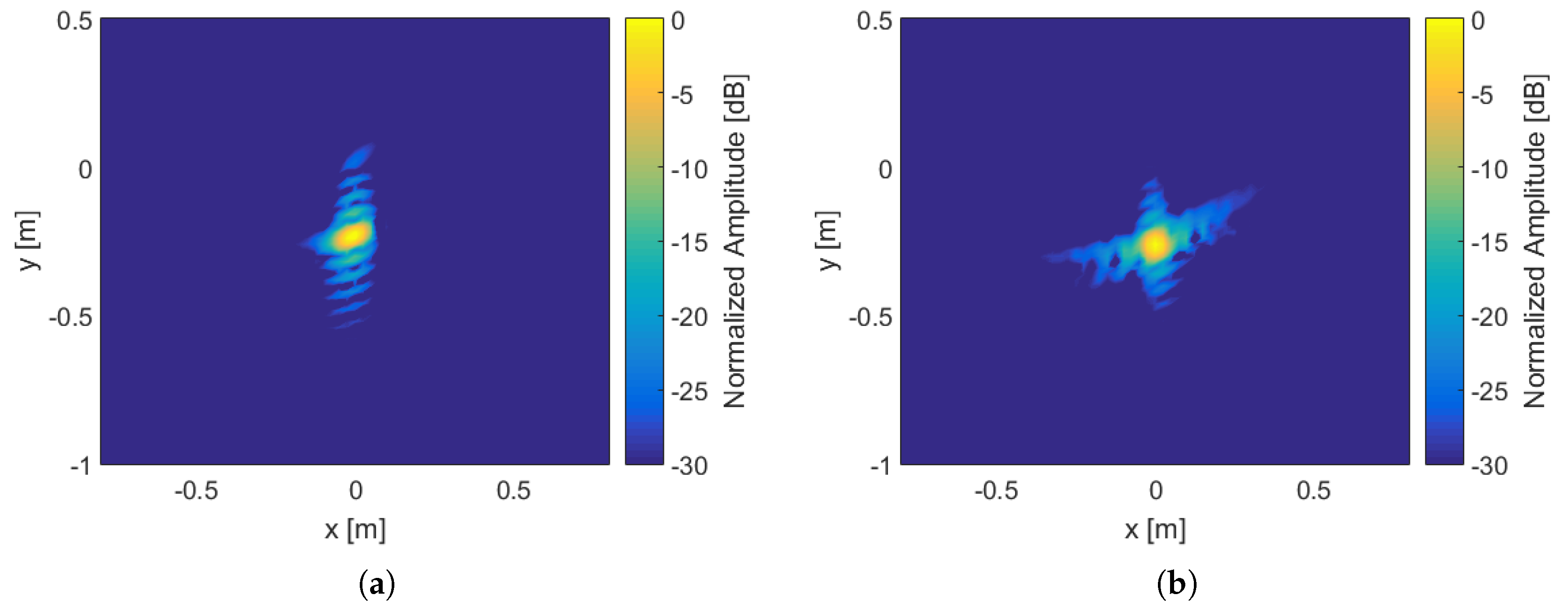
3.3.1. Multimonostatic Simulations
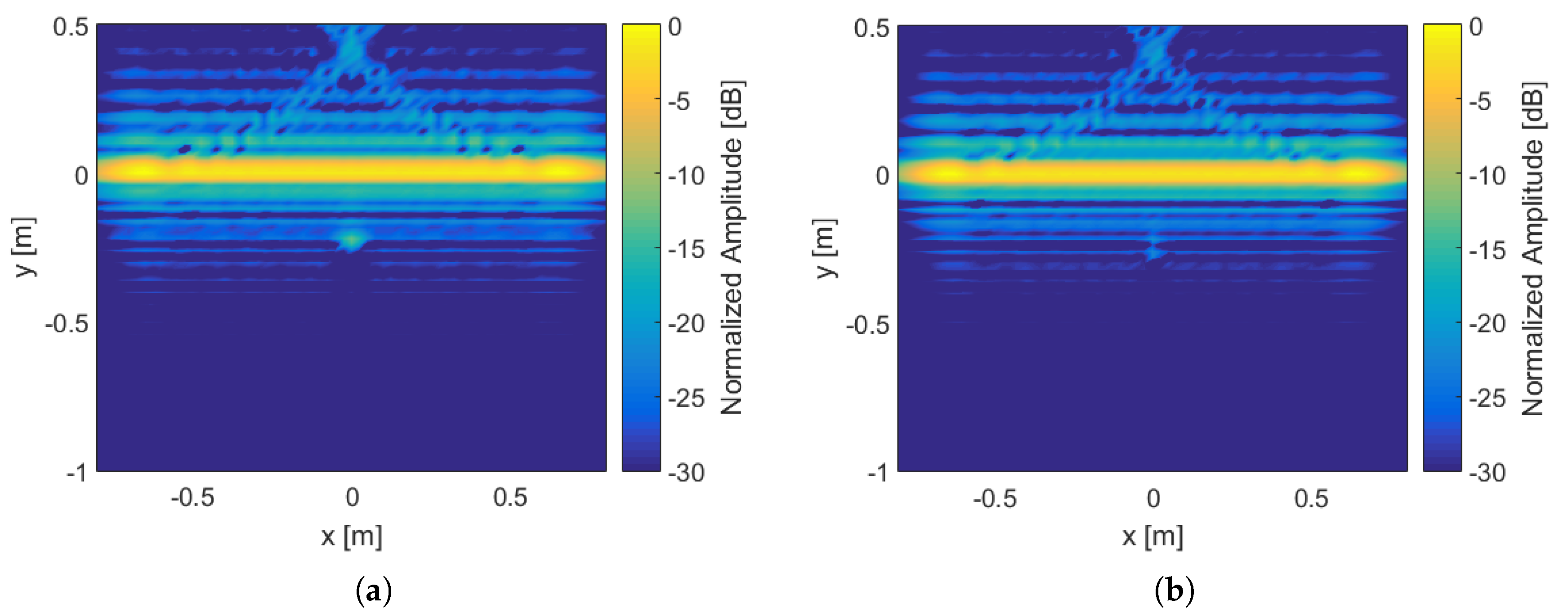
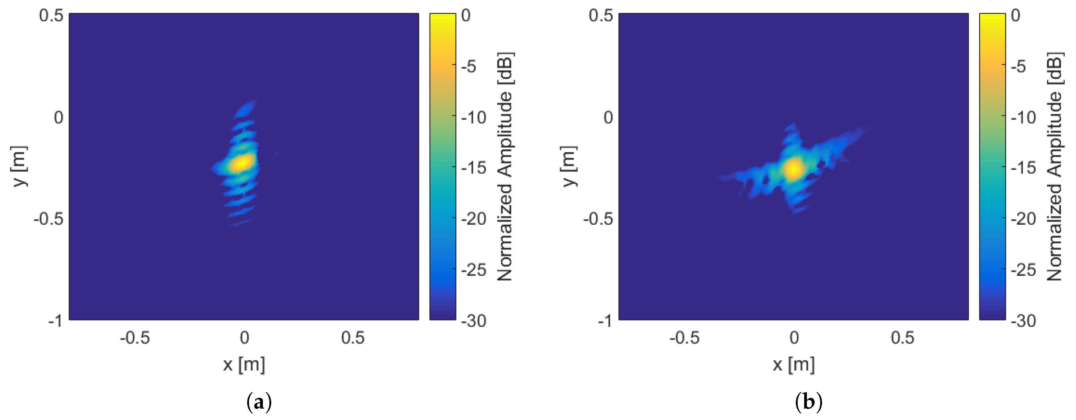
3.3.2. Multistatic and Multibistatic Simulations
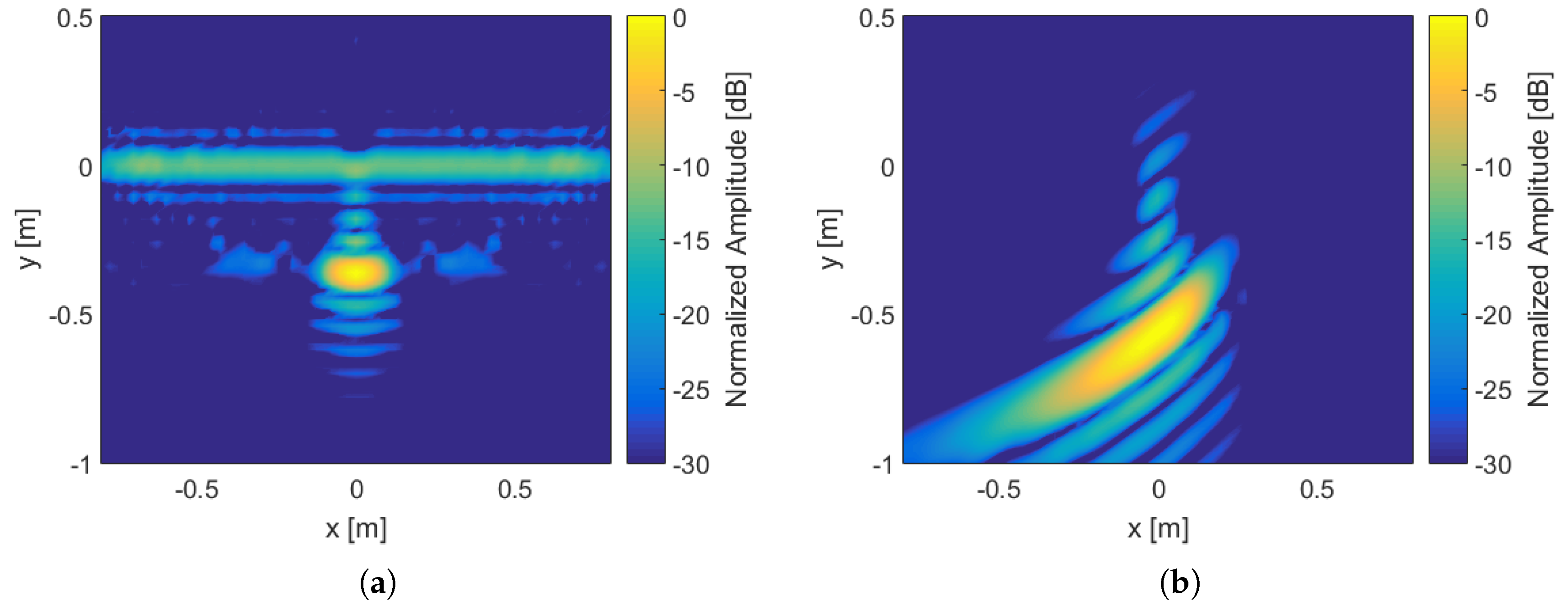
3.3.3. Effect of Inversion Path Length
3.4. Computational Performance
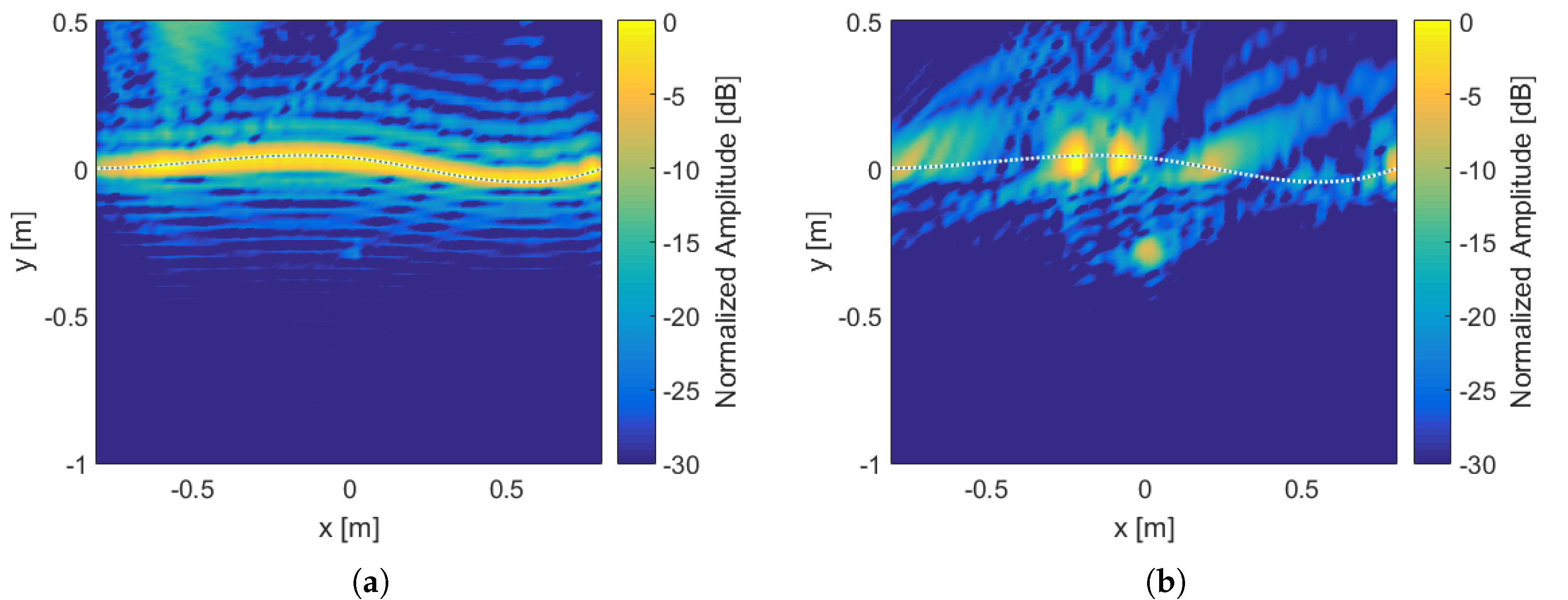
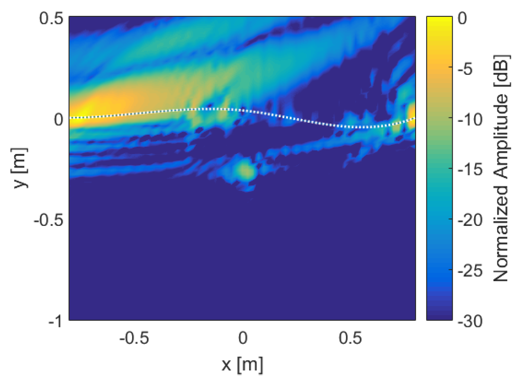
3.5. Effect of Rough Surface
3.6. Effect of Polarization
4. Analysis
5. Conclusions
Author Contributions
Funding
Conflicts of Interest
References
- Jol, H.M. Ground Penetrating Radar: Theory and Applications; Elsevier Science: Amsterdam, The Netherlands, 2008. [Google Scholar]
- Daniels, D. A Review of Landmine Detection Using GPR. In Proceedings of the European Radar Conference, Amsterdam, The Netherlands, 30–31 October 2008. [Google Scholar]
- Rappaport, C.; El-Shenawee, M.; Zhan, H. Suppressing GPR clutter from randomly rough ground surfaces to enhance nonmetallic mine detection. Subsurf. Sens. Technol. Appl. 2003, 4, 311–326. [Google Scholar] [CrossRef]
- Comite, D.; Ahmad, F.; Dogaru, T.; Amin, M.G. Adaptive Detection of Low-Signature Targets in Forward-Looking GPR Imagery. IEEE Geosci. Remote. Sens. Lett. 2018, 15, 1520–1524. [Google Scholar] [CrossRef]
- Rosen, E.M.; Ayers, E. Assessment of Down-Looking GPR Sensors for Landmine Detection. In Proceedings of the SPIE, Orlando, FL, USA, 10 June 2005. [Google Scholar]
- Garcia-Fernandez, M.; Alvarez-Lopez, Y.; Arboleya-Arboleya, A.; Gonzalez-Valdes, B.; Rodriguez-Vaqueiro, Y.; Las Heras, F.; Pino, A. Synthetic Aperture Radar imaging system for landmine detection using a Ground Penetrating Radar on board an Unmanned Aerial Vehicle. IEEE Access 2018, 6, 45100–45112. [Google Scholar] [CrossRef]
- Gonzalez-Valdes, B.; Alvarez-Lopez, Y.; Arboleya, A.; Rodriguez-Vaqueiro, Y.; Garcia-Fernandez, M.; Las Heras, F.; Pino, A. Airborne Systems and Methods for the Detection, Localisation and Imaging of Buried Objects, and Characterization of the Subsurface Composition. ES Patent 2577403 (WO2017/125627), 21 January 2016. [Google Scholar]
- Li, T.; Chen, K.-S.; Jin, M. Analysis and Simulation on Imaging Performance of Backward and Forward Bistatic Synthetic. Remote Sens. 2018, 10, 1676. [Google Scholar] [CrossRef]
- Balanis, C. Advanced Engineering Electromagnetics; Wiley: Hoboken, NJ, USA, 1989. [Google Scholar]
- Cai, J.; McMechan, G.A. Ray-based synthesis of bistatic ground-penetrating radar profiles. Geophysics 1995, 60, 87–96. [Google Scholar] [CrossRef]
- Williams, K.; Tirado, L.; Chen, Z.; Gonzalez-Valdes, B.; Martinez, J.A.; Rappaport, C.M. Ray Tracing for Simulation of Millimeter-Wave Whole Body Imaging Systems. IEEE Trans. Antennas Propag. 2015, 63, 5913–5918. [Google Scholar] [CrossRef]
- Rappaport, C.; Dong, Q.; Bishop, E.; Morghenthaler, A. Finite Difference Frequency Domain (FDFD) Modeling of Two Dimensional TE Wave Propagation and Scattering. In Proceedings of the URSI EMTS, Pisa, Italy, 23–27 May 2004. [Google Scholar]
- Ling, H.; Chou, R.C.; Lee, S.W. Shooting and bouncing rays: Calculating the RCS of an arbitrarily shaped cavity. IEEE Trans. Antennas Propag. 1989, 37, 194–205. [Google Scholar] [CrossRef]
- Zhan, Z.; Rappaport, C.; Farid, M.; Alshawabkeh, A.; Raemer, H. Born Approximation Model of Lossy Soil Half-Spaces: Cross-Well Radar Sensing Contaminants with Low-Order Parameter Optimization. IEEE Trans. Geosci. Remote Sens. 2007, 45, 2423–2429. [Google Scholar]
- Rappaport, C.; Kilmer, M.; Miller, E. Accuracy Considerations in Using the PML ABC with FDFD Helmholtz Equation Equation Computation. Int. J. Numer. Model. 2000, 13, 471–482. [Google Scholar] [CrossRef]
- Fuse, Y.; Gonzalez-Valdes, B.; Martinez-Lorenzo, J.A.; Rappaport, C.M. Advanced SAR Imaging Methods for Forward-Looking Ground Penetrating Radar. In Proceedings of the 10th European Conference on Antennas and Propagation (EuCAP), Davos, Switzerland, 10–15 April 2016. [Google Scholar]
- Morgenthaler, A.; Rappaport, C.M. Simple and accurate formulas for determining the refraction point and total path length from above ground to below ground points. in preparation.


| Method | Multimonostatic | Multistatic | Multibistatic |
|---|---|---|---|
| RT | 6.1 s | 0.5 s | 9.2 s |
| FDFD | 28.5 h | 32.2 min | 32.7 h |
© 2019 by the authors. Licensee MDPI, Basel, Switzerland. This article is an open access article distributed under the terms and conditions of the Creative Commons Attribution (CC BY) license (http://creativecommons.org/licenses/by/4.0/).
Share and Cite
Garcia-Fernandez, M.; Morgenthaler, A.; Alvarez-Lopez, Y.; Las Heras, F.; Rappaport, C. Bistatic Landmine and IED Detection Combining Vehicle and Drone Mounted GPR Sensors. Remote Sens. 2019, 11, 2299. https://doi.org/10.3390/rs11192299
Garcia-Fernandez M, Morgenthaler A, Alvarez-Lopez Y, Las Heras F, Rappaport C. Bistatic Landmine and IED Detection Combining Vehicle and Drone Mounted GPR Sensors. Remote Sensing. 2019; 11(19):2299. https://doi.org/10.3390/rs11192299
Chicago/Turabian StyleGarcia-Fernandez, Maria, Ann Morgenthaler, Yuri Alvarez-Lopez, Fernando Las Heras, and Carey Rappaport. 2019. "Bistatic Landmine and IED Detection Combining Vehicle and Drone Mounted GPR Sensors" Remote Sensing 11, no. 19: 2299. https://doi.org/10.3390/rs11192299