An Efficient Imaging Algorithm for GNSS-R Bi-Static SAR

Abstract

Global Navigation Satellite System Reflectometry (GNSS-R) based Bi-static Synthetic Aperture Radar (BSAR) is becoming more and more important in remote sensing, given its low power, low mass, low cost, and real-time global coverage capability. Due to its complex configuration, the imaging for GNSS-R BSAR is usually based on the Back-Projection Algorithm (BPA), which is very time consuming. In this paper, an efficient and general imaging algorithm for GNSS-R BSAR is presented. A Two Step Range Cell Migration (TSRCM) correction is firstly applied. The first step roughly compensates the RCM and Doppler phase caused by the motion of the transmitter, which simplifies the SAR data into the quasi-mono-static case. The second step removes the residual RCM caused by the motion of the receiver using the modified frequency scaling algorithm. Then, a cubic phase perturbation operation is introduced to equalize the Doppler frequency modulation rate along the same range cell. Finally, azimuth phase compensation and geometric correction are completed to obtain the focused SAR image. A simulation and experiment are conducted to demonstrate the feasibility of the proposed algorithm, showing that the proposed algorithm is more efficient than the BPA, without causing significant degradation in imaging quality.

1. Introduction

Global Navigation Satellite System Reflectometry (GNSS-R)uses the reflected GNSS signal to obtain information about the Earth’s surface, such as the speed of ocean winds [1,2], the soil moisture [3,4,5], the biomass of the land [5,6], the ocean altitude [7,8], etc. The concept of GNSS-R was firstly considered by Hall and Cordy in 1988 [9]. However, based on their erroneous estimates, they deemed this technique not very promising. In 1993, the concept for ocean altimetry using the GNSS reflected signal was proposed by Martin-Neira [10]. From then on, GNSS-R has achieved rapid development, both in the measurement concepts, instruments, and applications [11,12]. The first space borne GNSS-R mission, U.K. Disaster Monitoring Constellation (DMC), was launched in 2003 [13]. The Low Earth Orbiting U.K. TechDemoSat-1 satellite (TDS-1) was launched in 2014 [1]. The Cyclone Global Navigation Satellite System (CYGNSS) aimed to improve the prediction of extreme weather was launched by NASA in 2016 [14].

GNSS-R Bi-static Synthetic Aperture Radar (BSAR) is one of the new applications of the GNSS-R [15,16,17,18,19,20,21,22,23,24,25]. It uses the GNSS signal as a non-cooperative illuminator to obtain an image of the Earth’s surface. The advantage of GNSS-R BSAR is very significant compared with traditional SAR. Firstly, benefiting from the removal of the transmitting device, the GNSS-R system can be made low mass, low power, and low cost. Secondly, we can choose the GNSS satellites with different azimuth and elevation angles to observe the target from different perspectives. Thirdly, it can achieve easy synchronization aided by the GNSS time service [26]. Finally, it can achieve nearly real-time global monitoring due to the rich satellite resources. On the other hand, the GNSS-R BSAR also has some disadvantages. Firstly, the power of the GNSS signal is very low around the Earth’s surface, and thus, a longer integration time is needed to have a satisfactory Signal-to-Noise Rate (SNR) for the SAR image. Secondly, the instability of the illuminating power will lead to problems with the signal power calibration [27]. Another challenge for GNSS-R BSAR lies in efficient imaging. In general, two main difficulties are faced in the imaging of GNSS-R BSAR due to its complex geometry:

• The complex expression for range history: The range history is due to the motion of both the GNSS satellite and the receiving platform, which makes it extremely difficult to obtain a precise analytical solution to the stationary phase point of the Doppler phase.
• The translational variant Doppler history: Unlike mono-static SAR, the Doppler history of the echo signal of GNSS-R BSAR is translationally variant since the trajectories of the transmitter and the receiver are non-parallel and their velocities are also different. This means that imaging becomes a two-dimensional spatially varying filtering process.

As a result, commonly used imaging algorithms for GNSS-R BSAR are usually based on the Back-Projection Algorithm (BPA) [15,16,17,18,19,20,21,22,23]. Although having the ability of handling different configurations, these algorithms are very time consuming. In order to handle the spatial variation of the echo data, some two step algorithms [24,25] were proposed for GNSS-R BSAR. The general idea of those algorithms is very similar: a bulk compensation for coarse focusing and then a pointwise compensation for the residual RCM and phase error. These algorithms are proven to have better performance than the BPA. However, the second step for residual compensation is still inefficient. In [28], a Nonlinear Chirp Scaling (NCS) algorithm was presented to focus the SAR data collected in the translational variant mode for airborne BSAR. The key step is to equalize the Doppler Frequency Modulation (FM) rate using phase perturbation. This idea could potentially also be extended to the GNSS-R BSAR case.

In this paper, an accurate signal model is firstly established for GNSS-R BSAR. Then, the range history and Doppler phase history of the echo signal are analysed. Based on the analysis, an efficient imaging algorithm for GNSS-R BSAR is proposed. In the first step, the RCM and the Doppler phase caused by the motion of the transmitter are roughly removed through bulk compensation in the azimuth time domain. After this step, the bi-static SAR data are simplified into a quasi-mono-static case, so that precise expression of the echo data in the range-Doppler domain can be derived. In the range-Doppler domain, the RCM caused by the motion of the receiver and the residual RCM caused by the motion of the transmitter are corrected through the modified frequency scaling algorithm. Then, the data are transformed into the azimuth time domain, and phase perturbation is performed to equalize the Doppler FM rate along the same range cell. Finally, the data are transformed into the range-Doppler domain for azimuth phase compensation. In the whole procedure, only complex multiplications and FFT are needed, leading to a very efficient algorithm.

In order to demonstrate the feasibility and efficiency of the proposed imaging algorithm, point target simulation is firstly conducted. The GPS L5 satellite is chosen as the illuminator. The receiver is assumed to be moving along a nonparallel line to the satellite with different velocities. In total, 25 targets are laid out evenly in a 20 km × 20 km square area. The motion error of the receiver is ignored in our simulation. The imaging results of point targets at different locations are very consistent with theoretical analysis, demonstrating the feasibility of the proposed algorithm.

An experiment is also conducted to further confirm the feasibility of the proposed algorithm. Again, the GPS L5 satellite is chosen as the illuminator. The buildings at Beihang University are chosen as the imaging targets. The collected echo data are processed using the traditional BPA and the proposed algorithm, respectively. The imaging results are similar for the two algorithms, but the efficiency of the proposed algorithm is much higher than the traditional BPA. The imaging result is then compared with the optical image, and the strong scattering areas match the high density areas in the radar image well.

The paper is organized as follows: The signal model for GNSS-R BSAR and details of the proposed algorithm are presented in Section 2. Simulation and experimental results are provided in Section 3. A further discussion about the proposed algorithm is presented in Section 4, and conclusions are drawn in Section 5.

2. Materials and Methods

2.1. Modelling and Analysis

The general geometric configuration of the GNSS-R BSAR is shown in Figure 1. The receiver is mounted on an airplane moving in parallel to the ground along the x direction with a constant velocity V_r, and the transmitter is mounted on the GNSS satellite moving along its Kepler orbit. The target is positioned on the ground plane (x-y plane). The bi-static angle θ is defined as the angle between the target-to-satellite baseline and the target-to-receiver baseline. The receiver works in the broadside mode, and the beam centre of the receiver antenna falls at the y axis at t = 0. Here, t represents the azimuth slow time. The beam of the transmitter antenna covers most area of the Earth’s surface, and the antenna pattern is considered as constant in the imaging duration. For convenience of expression, in the following part of this paper, the slant range between the target and the satellite is referred to as the transmitter range, and the slant range between the target and the receiver is referred to as the receiver range.

For a typical SAR system, the transmitted signal is Linear Frequency Modulated (LFM). The GNSS system is not designed for SAR imaging application, and the structure of the transmitted signal is different from the LFM wave. For example, the GPS signal has three levels in structure: the bottom level is the carrier wave at the L-band; the middle level is the ranging codes, which are pseudorandom sequences; the upper level is the information code that carries the navigation message. For these three sequences, only the ranging code is used for imaging, and thus, the synchronization process should be performed firstly to cancel the other two sequences [15].

Assume the beam centre of the receiving antenna is focusing at target k at t = t₀. Then, the echo data of target k after synchronization and SAR data formation could be expressed as:

$$s\left(t,\tau \right)=a\left(t-t_0\right)C\left[\tau -\frac{R_k\left(t\right)}{c}\right]exp\left[-j2\pi \frac{R_k\left(t\right)}{\lambda }\right]$$

(1)

where a(t) is the antenna pattern of the receiver, C(τ) is the ranging code sequence, τ is the fast time, λ is the wavelength of the carrier, and c is the speed of light. R_k(t) is the total slant range, and R_k(t) = R_trk(t) + R_tsk(t). R_trk(t) is the receiver range for target k, and R_tsk(t) is the transmitter range for target k.

Assume that target k₀ has the same minimum transmitter range as target k. Then:

$$R_{trk}\left(t\right)=R_{trk0}\left(t-t_0\right),$$

(2)

$$s\left(t,\tau \right)=a\left(t-t_0\right)C\left[\tau -\frac{R_{trk0}\left(t-t_0\right)+R_{tsk}\left(t\right)}{c}\right]exp\left[-j2\pi \frac{R_{trk0}\left(t-t_0\right)+R_{tsk}\left(t\right)}{\lambda }\right]$$

(3)

The receiver range has the form of a hyperbola:

$$R_{trk0}\left(t\right)=\sqrt{R_{trk}^2+V_r^2{t}^2}$$

(4)

Using the Equivalent Slant Range Mode (ESRM) [29], the transmitter range can be expressed as:

$$R_{tsk}\left(t\right)=\sqrt{R_{tsk}^2\left(t_0\right)+V_0^2{sin}^2\phi {\left(t-t_0\right)}^2-2R_{tsk}\left(t_0\right)V_{0}sin\phi \left(t-t_0\right)}$$

(5)

where V₀ is the equivalent velocity and φ is the equivalent squint angle.

As can be seen from (3), (4), and (5), since the range history of the echo data for GNSS-R BSAR is caused by the motion of both the GNSS satellite and the airplane, the Doppler history of the echo data consists of two square roots. In this case, the stationary phase point does not have an analytical solution [30], and thus, the precise explicit expression of the echo data in the Range-Doppler (R-D) domain cannot be obtained. 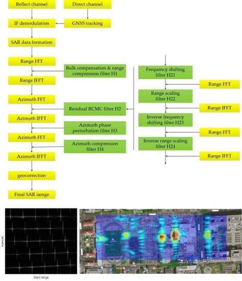Although the approximate R-D expression of the echo data for airborne BSAR and some associated imaging algorithms have been developed [31,32,33], the derivation is lengthy and tedious, and the accuracy of the approximation also decreases quickly when the bi-static angle increases. In this paper, a two step method is presented to get the R-D expression of the echo data more accurately for GNSS-R BSAR. It will be proven that the square root, which corresponds to the transmitter range, can be removed firstly by a bulk compensation. Then, the expression of the echo data is simplified into a quasi-mono-static case, which only has one square root. This process is referred to as slant range separation.

The slant range separation process is feasible due to the asymmetry between the transmitter range and the receiver range for GNSS-R BSAR. To show the details, we firstly take a look at the transmitter range. Again, GPS is chosen as an example.

The GPS orbit belongs to the high Earth orbit (HEO). The average altitude is about 20,200 km, and the orbit is very close to a circle. Since the altitude of the satellite is too high, if observed on the Earth’s surface, the spatial variation of the Doppler parameters of the GPS satellite is very slow. In fact, when the imaging scene is not too large and the integration time is not too long, the second and higher order components of the spatial variation of the transmitter range are negligible. It will be proven in the following by both theoretical derivation and simulation.

The orbit geometry of the GPS satellite is shown in Figure 2. The Doppler FM rate can be calculated by:

$$f_r=-\frac{V_s^2{cos}^2\phi }{\lambda R_{ts}}$$

(6)

Assuming that angle φ is constant for targets in the imaging scene, the directional derivative of f_r on the ground plane is:

$$\frac{d{f}_r}{d\overrightarrow{l}}=-\frac{V_s^2{cos}^2\phi }{\lambda }\left(\frac{-1}{R_{ts}^2}\right)\frac{d{R}_{ts}}{d\overrightarrow{l}}\le \frac{V_s^2{cos}^2\phi }{\lambda R_{ts}^2}\Vert grad\left(R_{ts}\right)\Vert =\frac{V_s^2{cos}^2\phi }{\lambda R_{ts}^2}cos\alpha$$

(7)

where $\Vert grad\left(R_{ts}\right)\Vert$ is the modulus of the gradient of R_ts on the ground plane, which is equal to the cosine of the elevation angle α of the satellite. When φ increases, $\frac{V_s^2{cos}^2\phi }{\lambda R_{ts}^2}$ decreases, and cosα increases. When φ increases to φ_max, cosα has the maximum value of one. Therefore:

$$\frac{d{f}_r}{d\overrightarrow{l}}<\frac{V_s^2}{\lambda R_{ts0}^2}$$

(8)

where R_ts0 is the height of the satellite relative to the ground when φ = 0 and V_s is the velocity of the satellite.

Then, the maximum range error caused by ignoring the second order component of the spatial variation of the transmitter range is:

$$er{r}_{range}=-\frac{\lambda }{2}max\left(\frac{d{f}_r}{d\overrightarrow{l}}\right)\frac{l}{2}{\left(\frac{T}{2}\right)}^2<-\frac{\lambda }{2}\frac{V_s^2}{\lambda R_{ts0}^2}\frac{l}{2}{\left(\frac{T}{2}\right)}^2$$

(9)

where T is the integration time and l is the size of the imaging scene.

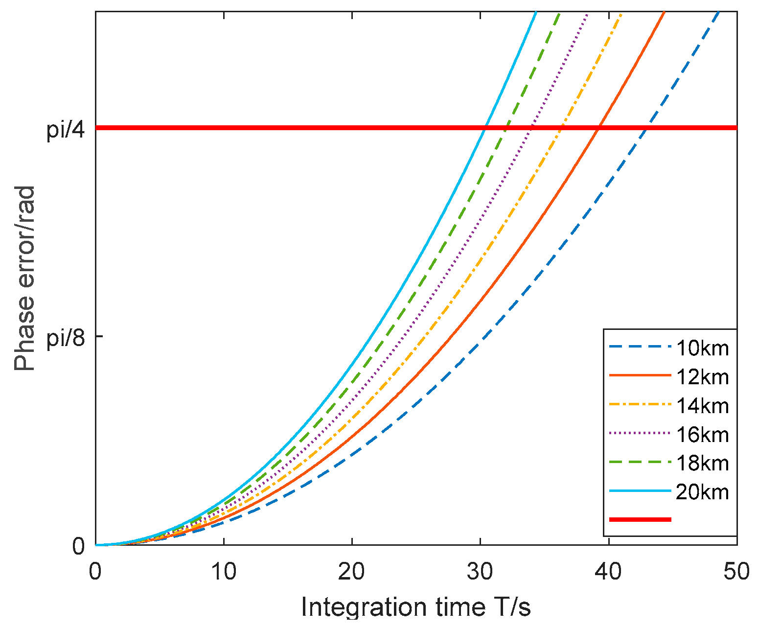
The corresponding phase error is:

$$er{r}_{phase}=\frac{-2\pi er{r}_{range}}{\lambda }<\pi \frac{V_s^2}{\lambda R_{ts0}^2}\frac{l}{2}{\left(\frac{T}{2}\right)}^2$$

(10)

The simulation result is shown in Figure 3. The six curves correspond to the maximum phase error as a function of integration time for different sizes of the scene (10 km to 20 km with a linear spacing of 2 km from the bottom to the top). The red straight line corresponds to the π/4 phase error criterion for the GPS L5 carrier. It can be seen that, for an imaging scene no larger than 20 km × 20 km, the phase error caused by the second and higher order components of the spatial variation of the transmitter range is still acceptable even when the integration time reaches 30 s. Thus, if a bulk compensation for the transmitter range using the scene centre as the reference point is firstly applied, the residual transmitter range has only a fixed linear component. Then, the expression of the echo data is simplified into a quasi-mono-static case, which only has one square root, and the stationary phase point can then be calculated analytically.

After the bulk compensation for transmitter range, the echo signal for target k₀ becomes:

$$s\left(t,\tau \right)=a\left(t-t_0\right)C\left\{\tau -\frac{R_{trk0}\left(t-t_0\right)+R_{tsk}\left(t\right)-R_{tsc}\left(t\right)}{c}\right\}exp\left\{-j2\pi \frac{R_{trk0}\left(t-t_0\right)+R_{tsk}\left(t\right)-R_{tsc}\left(t\right)}{\lambda }\right\}$$

(11)

where R_tsc(t) is the transmitter range for target c, which is positioned at the centre of the scene.

Expanding $R_{tsk}\left(t\right)-R_{tsc}\left(t\right)$ at t = 0 and keeping only those up to the first order, we have:

$$\begin{array}{cc}\hfill R_{tsk}\left(t\right)-R_{tsc}\left(t\right)& \approx R_{tsk}-R_{tsc}-\lambda \left(f_{dk}-f_{dc}\right)t\hfill \\ & \approx R_{tsk}-R_{tsc}-\lambda \frac{\partial f_d}{\partial x}{x}_0{t}_0-\lambda \frac{\partial f_d}{\partial y}{y}_0{t}_0-\lambda \left(\frac{\partial f_d}{\partial x}{x}_0+\frac{\partial f_d}{\partial y}{y}_0\right)\left(t-t_0\right)\hfill \\ & =R_{tsk0}-R_{tsc}+R_{shiftk}-\lambda \mathsf{\Delta }{f}_{dk}\left(t-t_0\right)\hfill \end{array}$$

(12)

where:

$$R_{tsk}=R_{tsk}\left(t=0\right),R_{tsc}=R_{tsc}\left(t=0\right),R_{tsk0}=R_{tsk0}\left(t=0\right),$$

(13)

$$R_{shiftk}=R_{tsk}-R_{tsk0}-\lambda \frac{\partial f_d}{\partial x}{x}_0{t}_0-\lambda \frac{\partial f_d}{\partial y}{y}_0{t}_0,$$

(14)

$$\mathsf{\Delta }{f}_{dk}={\frac{\partial f_d}{\partial x}{x}_0+\frac{\partial f_d}{\partial y}{y}_0|}_{\left(x,y\right)=\left(0,0\right)}$$

(15)

R_shiftk is the position shift of the signal in the echo window. The Doppler frequency f_d and its derivative can be expressed as a function of the parameters of the satellite and the target.

$$\begin{gathered} f_d=-\frac{\overrightarrow{V_s}\cdot \overrightarrow{R_{ts}}}{\lambda R_{ts}} \\ \frac{\partial f_d}{\partial x}=\frac{\overrightarrow{V_s}\cdot \overrightarrow{i_x}}{\lambda R_{ts}}-\frac{\overrightarrow{V_s}\cdot \overrightarrow{R_{ts}}}{\lambda R_{ts}^2}\left(\overrightarrow{i_{rts}}\cdot \overrightarrow{i_x}\right) \\ \frac{\partial f_d}{\partial y}=\frac{\overrightarrow{V_s}\cdot \overrightarrow{i_y}}{\lambda R_{ts}}-\frac{\overrightarrow{V_s}\cdot \overrightarrow{R_{ts}}}{\lambda R_{ts}^2}\left(\overrightarrow{i_{rts}}\cdot \overrightarrow{i_y}\right) \end{gathered}$$

(16)

where $\overrightarrow{i_x}$ is the unit directional vector of the x axis, $\overrightarrow{i_y}$ is the unit directional vector of the y axis, and $\overrightarrow{i_{rts}}$ is the unit directional vector from the target to the satellite.

Substituting (12) into (11) leads to:

$$\begin{array}{cc}\hfill s\left(t,\tau \right)& =a\left(t-t_0\right)C\left\{\tau -\frac{R_{k0}\left(t-t_0\right)+R_{shiftk}-\lambda \mathsf{\Delta }{f}_{dk}\left(t-t_0\right)}{c}\right\}\exp \left\{-j2\pi \frac{R_{k0}\left(t-t_0\right)-\lambda \mathsf{\Delta }{f}_{dk}\left(t-t_0\right)}{\lambda }+{\phi }_1\right\}\hfill \\ & \approx a\left(t-t_0\right)C\left\{\tau -\frac{R_{k0}\left(t-t_0-t_{dk}\right)+R_{shiftk}}{c}\right\}\exp \left\{-j2\pi \frac{R_{k0}\left(t-t_0-t_{dk}\right)}{\lambda }\right\}\hfill \end{array}$$

(17)

where:

$$R_{k0}\left(t\right)=R_{trk0}\left(t\right)+R_{tsk0}-R_{tsc}$$

(18)

The last approximation holds when the scene size and integration time are not too large.

$$t_{dk}=\frac{\mathsf{\Delta }{f}_{dk}}{k_a}=-\frac{\lambda R_{trk}\mathsf{\Delta }{f}_{dk}}{V_r^2}$$

(19)

where k_a is the Doppler FM rate for target k caused by the motion of the receiver. The phase φ₁ is omitted because it has no impact on the derivation.

For mono-static SAR, the echo data for targets with the same minimum slant range have the same Doppler history and RCM curve. This means the echo data are translationally invariant. Thus, the imaging algorithms in the azimuth frequency domain are usually more efficient. Due to the non-parallel trajectory and different velocity of the transmitter and the receiver, the echo data for GNSS-R BSAR are translationally variant. This property can be observed by (17) in two aspects.

• The spatially varying Doppler centroid: It is formed by the linear component of the residual transmitter range and represented by the spatially varying delay time t_dk. This means the equivalent squint angle is also spatially varying.
• The translational variant Doppler FM rate: It is formed by the constant component of the residual transmitter range and represented by the shifting factor R_shiftk. The shifting factor R_shiftk indicates that the echo data for targets with the same minimum receiver range (thus the same Doppler FM rate) will not appear in the same range cell. In other words, the signals that appear in the same range cell have a different Doppler FM rate.

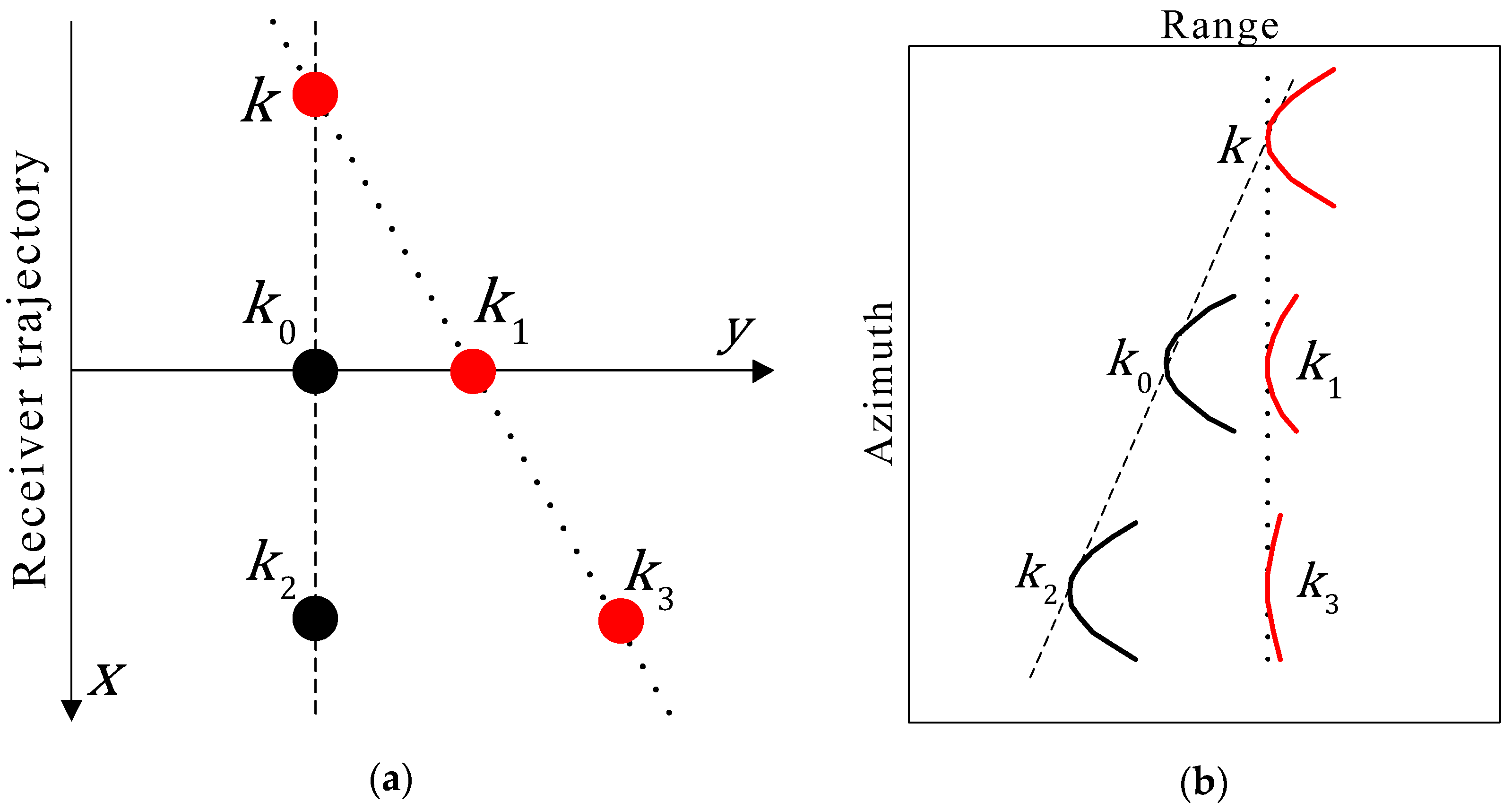
To illustrate the range cell shift effect of the shifting factor, two spaces are defined for GNSS-R BSAR, as shown in Figure 4.

• The scene space in which the echo data are received.
• The echo space in which the echo data are stored and processed.

As can be seen from the figure, due to the effect of the shifting factor R_shiftk, for targets with the same minimum receiver range (thus the same Doppler FM rates since they are caused only by the motion of the receiver after bulk compensation for transmitter range) in the scene space, their echo data will not appear in the same range cell in the echo space. In other words, for the echo data in the same range cell, their Doppler FM rates are different. As an example, target k has the same minimum receiver range as target k₀ and thus has the same Doppler FM rate as target k₀. However, the echo data of target k appear in the same range cell as target k₁ rather than target k₀ in the echo space, since $R_k\left(t_0\right)+R_{\mathrm{shiftk}}=R_{k_0}\left(0\right)+R_{\mathrm{shiftk}}=R_{k_1}\left(0\right)$.

In order to focus the echo data efficiently in the R-D domain, the Doppler FM rate in the same range cell needs to be equalized. Here, the term “equalize” means making the Doppler FM rates equal. Firstly, we consider the shifting curve R_shiftk.

The first term of R_shiftk is caused by the difference in transmitter range for different targets at t = 0. This term is positively related to the bi-static angle θ. Since θ varies widely in different receiving geometry, this term also varies widely and in general is also the dominating term of R_shiftk. This term is a linear function of the azimuth time. The second term is caused by the variation of the Doppler frequency along the direction of the receiver velocity, and this is a quadratic function of the azimuth time. The third term is caused by the variation of the Doppler frequency along the cross direction of the receiver velocity, and it is also a linear function of the azimuth time, but the slope varies with y₀.

The latter two terms are a function of x₀ and y₀, which are negligible when the imaging scene is not too large. Ignoring the second term, we have:

$$R_{shiftk}\approx \frac{\partial R_{ts}}{\partial x}{V}_r{t}_0-\lambda \frac{\partial f_d}{\partial y}{y}_0{t}_0$$

(20)

which is a linear function of the azimuth time.

Correspondingly, for targets whose echo data appear in the same range cell, the minimum receiver range is:

$$\begin{array}{cc}\hfill R_{tr}\left(t\right)& =R_{trk}+\frac{\partial R_{tr}}{\partial R}{R}_{shiftk}\hfill \\ & =R_{trk}\left(1+\frac{\partial R_{tr}}{\partial R}\frac{\frac{\partial R_{ts}}{\partial x}{V}_r-\lambda \frac{\partial f_d}{\partial y}{y}_0}{R_{trk}}t\right)\hfill \\ & =R_{trk}\left(1+\gamma t\right)\hfill \end{array}$$

(21)

where:

$$\frac{\partial R_{tr}}{\partial R}=\frac{\frac{\partial R_{tr}}{\partial y}}{\frac{\partial R}{\partial y}},$$

(22)

$$\gamma =\frac{\partial R_{tr}}{\partial R}\frac{\frac{\partial R_{ts}}{\partial x}{V}_r-\lambda \frac{\partial f_d}{\partial y}{y}_0}{R_{trk}}$$

(23)

Then, the Doppler FM rate along the same range cell is:

$$k\left(t\right)=\frac{-V_r^2}{\lambda R_{tr}\left(t\right)}=\frac{-V_r^2}{\lambda R_{trk}\left(1+\gamma t\right)}\approx \frac{-V_r^2}{\lambda R_{trk}}\left(1-\gamma t\right)=\frac{-V_r^2}{\lambda R_{trk}}+\frac{V_r^2}{\lambda R_{trk}}\gamma t=k_a+\mathsf{\Delta }k\left(t\right),$$

(24)

$$\mathsf{\Delta }k\left(t\right)=\frac{V_r^2}{\lambda R_{trk}}\gamma t=\frac{V_r^2\left(\frac{\partial R_{ts}}{\partial x}{V}_r-\lambda \frac{\partial f_d}{\partial y}{y}_0\right)\frac{\partial R_{tr}}{\partial R}}{\lambda R_{trk}{}^2}t$$

(25)

It can be seen that the Doppler FM rate along the same range cell is approximately a linear function of the azimuth time. Therefore, a cubic perturbation function is sufficient to equalize the Doppler FM rate along the range cell.

2.2. Imaging Methods

Based on the above analysis, an efficient and general imaging algorithm is proposed for GNSS-R BSAR. The block diagram of the proposed algorithm is shown in Figure 5.

Firstly, two receiving channels are used to collect the reflected signal and the direct signal, respectively. The reflected channel signal is used for imaging, whereas the direct channel signal is used for positioning and synchronization. This step is introduced to track the time delay, phase, and navigation message of the GNSS signal and eliminate the phase error caused by clock slippage and local oscillator drift of the receiver [15].

Then, the signal is truncated to form the SAR data. The echo data of target k after synchronization and SAR data formation can be expressed as (11).

2.2.1. Bulk Compensation and Range Compression

Fast Fourier Transform (FFT) along the range direction is performed, and bulk compensation for transmitter range along with range compression is accomplished in the range frequency domain. The expression of the bulk compensation and range compression filter function is given by:

$$H_{brc}=F^{*}\left(f_{\tau }\right)exp\left[j2\pi \frac{f_0+f_{\tau }}{c}{R}_{tsc}\left(t\right)\right]$$

(26)

where $F^{*}\left(f_{\tau }\right)$ is the complex conjugate of the Fourier transform of C(τ). Then, the data are transformed into the time domain by performing the range IFFT, and the signal becomes:

$$s_1\left(t,\tau \right)=a\left(t-t_0\right)P\left\{\tau -\frac{R_{k0}\left(t-t_0-t_{dk}\right)+R_{shiftk}}{c}\right\}exp\left\{-j2\pi \frac{R_{k0}\left(t-t_0-t_{dk}\right)}{\lambda }\right\}$$

(27)

where P(τ) is the auto-correlation function of the GNSS ranging code. The data are then transformed into the range-Doppler domain.

2.2.2. Residual RCMC

Due to the different equivalent squint angle caused by the linear component of the residual transmitter range, the Range Cell Migration (RCM) of the data in the same range cell has different slope in the azimuth time domain. However, they should still satisfy the same RCM curve in the range-Doppler domain, just corresponding to different intervals, and thus can be corrected uniformly according to the reference point, which is chosen to have a zero equivalent squint angle and thus a zero delay time t_d.

In traditional SAR applications, the chirp scaling algorithm is often used to correct the range cell variant RCM of the SAR data. However, in GNSS-R BSAR, the transmitted signal is not a chirp signal, and thus, the chirp scaling algorithm is no longer suitable. The Frequency Scaling (FS) algorithm was introduced in [34] to correct the RCM of the de-ramped signal for spotlight SAR. In this paper, it will be proven that after some changes, this algorithm is also capable of handling the RCM Correction (RCMC) problem for GNSS-R BSAR:

• The scaling operation is not applied to the range frequency axis, but to the range time axis, and thus in some sense, it is more appropriate to name the modified algorithm the range scaling algorithm rather than the frequency scaling algorithm.
• The scaling of the range time needs four multiplications rather than three as in the frequency scaling algorithm.
• The scaling factors should all be adapted to the new application.

The detail of the residual RCMC process is illustrated in the following. Firstly, the RCM caused by the motion of the receiver and the residual RCM caused by the motion of the transmitter are equalized by the so-called range scaling algorithm. This step is a combination of four sequential processes: frequency shift, range scaling, inverse frequency shift, and inverse range scaling. After these four operations, the RCM of the signal at different range cells is equalized, and then, a bulk RCMC is applied to finish correcting the RCM.

Considering the reference point for target k₀ (note that the reference point is not always located at the y axis, and target k₀ has a non-zero equivalent squint angle), the echo data of the reference point after bulk compensation for transmitter range have the following form:

$$s_{ref}\left(t,\tau \right)=a\left(t-t_{ref}\right)P\left[\tau -\frac{R_{trk0}\left(t\right)+R_{tsk0}-R_{tsc}}{c}\right]exp\left[-j2\pi \frac{R_{trk0}\left(t\right)+R_{tsk0}-R_{tsc}}{\lambda }\right]$$

(28)

The RCM in the azimuth time domain is given by:

$$RCM\left(t\right)=R_{trk0}\left(t\right)+R_{tsk0}-R_{tsc}$$

(29)

Transformed into the range-Doppler domain, the RCM becomes:

$$\begin{array}{cc}\hfill RCM\left(f\right)& =R_{trk0}\left[t\left(f\right)\right]+R_{tsk0}-R_{tsc}\hfill \\ & =\frac{R_{trk0}-R_{trc}}{D_f}+\frac{R_{trc}}{D_f}+R_{tsk0}-R_{tsc}\hfill \\ & \approx \frac{R_{k0}-R_c}{D_f}\frac{\partial R_{tr}}{\partial R}+\frac{R_{trc}}{D_f}+\left(1-\frac{\partial R_{tr}}{\partial R}\right)\left(R_{k0}-R_c\right)\hfill \\ & =\frac{\left(R_{k0}-R_c\right)}{\beta }+\alpha R_{trc}\hfill \end{array}$$

(30)

where:

$$\begin{gathered} R_{trk0}=R_{trk0}\left(0\right) \\ {D}_f=\sqrt{1-{\left(\frac{\lambda f}{V_r}\right)}^2} \\ t\left(f\right)=\frac{\frac{-\lambda R_{trk0}f}{V_r^2}}{D_f} \\ \alpha =\frac{1}{D_f} \\ \beta =\frac{1}{\left[\frac{\partial R_{tr}}{\partial R}\left(\alpha -1\right)+1\right]} \end{gathered}$$

(31)

Thus, the RCMC can be accomplished by two main steps: scaling the range time axis by β times, followed by a bulk RCMC to correct the equalized RCM αβR_trc. The four scaling filter functions corresponding to the first step are:

$$\begin{gathered} H_{fs}=exp\left(j\pi k{\tau }^2\right) \\ {H}_{rs}=exp\left(\frac{j\pi f_{\tau }^2\left(1-\beta \right)}{k}\right) \\ {H}_{ifs}=exp\left(\frac{-j\pi k{\tau }^2}{\beta }\right) \\ {H}_{irs}=exp\left(\frac{-j\pi f_{\tau }^2\beta \left(1-\beta \right)}{k}\right) \end{gathered}$$

(32)

Here, the subscripts in the four filter functions represent frequency shift, range scaling, inverse frequency shift, and inverse range scaling, respectively. The first multiplication is performed to shift the range frequency of the echo data according to their RCM. After this, the base-band range signal is modulated by a different frequency according to their RCM. The 2D frequency spectrum has a similar curve as the RCM along the azimuth direction, and the range scaling multiplication is then performed. The factor k in the frequency shift filter function H_fs is not fixed, but it should make sure that the spectrum shift does not surpass the sampling rate. The purpose of the next three filter functions is similar to their counterparts in the frequency scaling algorithm. For a detailed description of their functions, please refer to [34]. The final bulk RCMC filter function is given by:

$$H_{bulk}=exp\left(\frac{j2\pi f_{\tau }\alpha \beta R_{trc}}{c}\right)$$

(33)

This filter function can be incorporated into the inverse frequency shift filter function in practice, given by:

$$H_{irs}=exp\left(\frac{-j\pi f_{\tau }^2\beta \left(1-\beta \right)}{k}\frac{+j2\pi f_{\tau }\alpha \beta R_{trc}}{c}\right)$$

(34)

Note that in our analysis, we removed the range cell shift of the targets from the reference point. This will cause a small error in the RCM correction for those targets. However, since the range cell shift is so small in terms of RCM spatial variation, this error is actually negligibly small.

2.2.3. Azimuth Phase Perturbation

After residual RCMC, the RCM of the echo data is corrected. The data are then transformed into the azimuth time domain. The expression of the data after residual RCMC for target k becomes:

$$s_2\left(t,\tau \right)=a\left(t-t_0\right)\beta P\left[\frac{1}{\beta }\left(\tau -\frac{R_k+R_{shiftk}}{c}\right)\right]exp\left\{-j2\pi \frac{R_{k0}\left(t-t_0-t_{dk}\right)}{\lambda }\right\},$$

(35)

$$R_k=R_{trk0}+R_{tsk0}-R_{tsc}$$

(36)

Since β is very close to one, the broadening of the range profile is negligible, and then:

$$s_2\left(t,\tau \right)=a\left(t-t_0\right)P\left(\tau -\frac{R_k+R_{shiftk}}{c}\right)exp\left[-j2\pi \frac{R_{k0}\left(t-t_0-t_{dk}\right)}{\lambda }\right]$$

(37)

As shown in our earlier analysis, the cubic phase perturbation function is sufficient to equalize the Doppler FM rate along the range cell. Considering the expression of Δk, the expression of the perturbation function should be:

$$H_{perturbation}=exp\left[j\pi \frac{V_r^2\left(\frac{\partial R_{ts}}{\partial x}{V}_r-\lambda \frac{\partial f_d}{\partial y}{y}_0\right)\frac{\partial R_{tr}}{\partial R}}{3\lambda R_{trk}{}^2}{t}^3\right]$$

(38)

In addition to equalizing the Doppler FM rate along the range cell, the perturbation filter function also has some side effects. The effect of the components with different orders in the perturbation filter function is analysed below.

• The constant component πat₀³: It changes the phase of the signal according to the position of the target, which can be ignored when only the amplitude of the image is concerned. Here:

  $$a=\frac{V_r^2\left(\frac{\partial R_{ts}}{\partial x}{V}_r-\lambda \frac{\partial f_d}{\partial y}{y}_0\right)\frac{\partial R_{tr}}{\partial R}}{3\lambda R_{trk}{}^2},$$

  (39)

  $$t_0=\frac{x_0}{V_r}$$

  (40)
• The first order component 3πat₀²(t − t₀): It adds a small spatially varying Doppler shift to the signal. This shift is a quadratic function of the azimuth time t, which can be incorporated into the Doppler shift caused by the residual transmitter range, i.e.,

  $$\mathsf{\Delta }{f}_{dk}=\frac{\partial f_d}{\partial x}{x}_0+\frac{\partial f_d}{\partial y}{y}_0-\frac{\left(\frac{\partial R_{ts}}{\partial x}{V}_r-\lambda \frac{\partial f_d}{\partial y}{y}_0\right)\frac{\partial R_{tr}}{\partial R}}{2\lambda R_{trk}{}^2}{x}_0^2$$

  (41)
• The second order compound 3πat₀(t − t₀) ²: It equalizes the Doppler FM rate along the range cell.
• The third order compound πa(t − t₀)³: It is a cubic phase modulation, which is the same for all targets. It is far smaller than the phase modulation caused by the receiver motion, which can be ignored during the derivation of the azimuth stationary phase point of the signal.

2.2.4. Azimuth Compensation

After applying the phase perturbation, the second and higher order components of the echo data along the same range cell are equalized, and thus, those data can be focused by the same azimuth compensation filter function. Considering the reference target k₀, the expression of the echo data of target k₀ after phase perturbation is:

$$s_{k0}\left(t,\tau \right)=a\left(t\right)P\left(\tau -\frac{R_{k0}}{c}\right)exp\left[-j2\pi \frac{R_{k0}\left(t\right)-\frac{\lambda \mathsf{\Delta }{f}_{dk0}t-\lambda a{t}^3}{2}}{\lambda }\right]$$

(42)

where:

$$\mathsf{\Delta }{f}_{dk0}=\frac{\partial f_d}{\partial y}{y}_0$$

(43)

The method of the stationary phase is applied to calculate the expression of the echo data for the reference target k₀ in the range-Doppler domain. Ignoring the cubic phase modulation caused by the phase perturbation during the derivation of the stationary phase point, we have:

$$t\left(f\right)=\frac{\frac{-\lambda R_{trk0}}{V_r^2\left(f-\mathsf{\Delta }{f}_{dk0}\right)}}{\sqrt{1-{\left[\frac{\lambda \left(f-\mathsf{\Delta }{f}_{dk0}\right)}{V_r}\right]}^2}},$$

(44)

$$s_{k0}\left(f,\tau \right)=a\left[t\left(f\right)\right]P\left(\tau -\frac{R_{k0}}{c}\right)exp\left[-j2\pi \frac{R_{k0}\left[t\left(f\right)\right]-\frac{\lambda \mathsf{\Delta }{f}_{dk0}t\left(f\right)-\lambda a{t}^3\left(f\right)}{2}}{\lambda }-j2\pi ft\left(f\right)\right]$$

(45)

The azimuth compensation filter function is chosen as:

$$\begin{array}{cc}\hfill H_{ac}& =\exp \left[j2\pi \frac{R_{k0}\left[t\left(f\right)\right]-\lambda \mathsf{\Delta }{f}_{dk0}t\left(f\right)-\lambda a{t}^3\left(f\right)/2}{\lambda }+j2\pi ft\left(f\right)\right]\hfill \\ & =\exp \left\{j2\pi \left[\begin{array}{l}\sqrt{R_{trk0}^2+V_r^2{t}^2\left(f\right)}+R_{tsk0}-R_c-\lambda \mathsf{\Delta }{f}_{dk0}t\left(f\right)\\ -\frac{V_r^2\left(\frac{\partial R_{ts}}{\partial x}{V}_r-\lambda \frac{\partial f_d}{\partial y}{y}_0\right)\frac{\partial R_{tr}}{\partial R}}{6R_{trk}{}^2}{t}^3\left(f\right)\end{array}\right]/\lambda +j2\pi ft\left(f\right)\right\}\hfill \end{array}$$

(46)

The azimuth compensation is accomplished by multiplication of the echo signal with the azimuth compensation filter function. Then, the data are transformed into the time domain by the inverse FFT to obtain the focused SAR image. For target k, it is:

$$s_3\left(t,\tau \right)=AP\left(\tau -\frac{R_k+R_{shiftk}}{c}\right)\sin \mathrm{c}\left[B\left(t-t_0-t_d\right)\right]$$

(47)

where:

$$\sin \mathrm{c}\left(t\right)=\frac{sin\left(\pi t\right)}{\pi t},$$

(48)

$$t_d=\frac{\mathsf{\Delta }{f}_{dk}-\mathsf{\Delta }{f}_{dk0}}{k_a}=-\frac{\lambda R_{trk}}{V_r^2}\left(\frac{\partial f_d}{\partial x}{x}_0-\frac{\left(\frac{\partial R_{ts}}{\partial x}{V}_r-\lambda \frac{\partial f_d}{\partial y}{y}_0\right)\frac{\partial R_{tr}}{\partial R}}{2\lambda R_{trk}{}^2}{x}_0^2\right)$$

(49)

3. Results

3.1. Simulation Results

Simulations were conducted to demonstrate the performance of the proposed algorithm. The geometric relations of the satellite and the receiver are shown in

Table 1. The geometric relations of the simulation.

	x	y	z
Satellite position (km)	−5908	−12,714	16,112
Satellite velocity (m/s)	−2475	−1198	−1310
Receiver position (m)	0	0	6000
Receiver velocity (m/s)	60	0	0

. Some parameters used in the simulation are listed in

Table 2. Parameters used in the simulation.

Satellite/Signal	GPS L5
Carrier frequency	1176.45 MHz
Signal bandwidth	10.23 MHz
Sample rate	40 MHz
Integration time	10 s

.

An array of 25 targets were considered, which were laid out on a square area of 20 km × 20 km, as shown in Figure 6a, and the imaging results using the proposed algorithm are shown in Figure 6b. The bi-static angle θ was about 25 degrees, and the angle between the target velocity and the transmitter velocity was about 26 degrees. A rectangular antenna pattern was assumed in both the azimuth and range directions.

The GPS L5 satellite was chosen as the illuminator, and the ranging code sequence of the GPS L5 signal and its auto-correlation sequence are shown in Figure 7.

The imaging results of five chosen targets (Targets 1, 7, 13, 19, and 25) are presented in Figure 8. As can be seen, Targets 7, 13, and 19 were well focused. The range profile and the azimuth profile were well consistent with theoretical ones. For Targets 1 and 25, slight degradation can be observed in the azimuth profile. This is also consistent with our analysis, since Targets 1 and 25 were positioned at the edge of the scene, where the quadratic part of the range cell shift reached its maximum value (about 184 m in the simulation). Thus, Targets 1 and 25 suffered from the most severe Doppler FM rate mismatch, which resulted in distortion in the azimuth profile. The evaluation results are listed in

Table 3. Evaluation results for the chosen targets. ISLR, Integrated Side-Lobe Ratio.

Target	Range			Azimuth
	Resolution (m)	PSLR (dB)	ISLR (dB)	Resolution (m)	PSLR (dB)	ISLR (dB)
1	17.1	−32.92	−14.53	9.9	−12.97	−10.50
7	16.7	−34.76	−13.47	9.7	−13.24	−10.83
13	16.5	−34.68	−13.45	9.6	−13.27	−10.90
19	16.6	−35.04	−13.47	9.8	−13.21	−10.89
25	16.9	−33.85	−13.65	10.1	−12.90	−10.59
Theoretical	16.5	−35.00	−13.45	9.6	−13.26	−10.90

. For Targets 7, 13, and 19, the degradation in the Peak Side-Lobe Ratio (PSLR) and Integrated Side-Lobe Ratio (ISLR) was in fact negligible. For Targets 1 and 25, the degradation in azimuth PSLR was 0.29 dB and 0.36 dB, respectively, and the degradation in azimuth ISLR was 0.40 dB and 0.31 dB, respectively.

An azimuth variant rotation in the range side-lobe can be observed in the 2D contour of the imaging results. This was caused by the linear component of the spatially varying residual transmitter range. It can also be considered as the system having a spatially varying equivalent squint angle.

The azimuth resolution for GNSS-R BSAR was mainly determined by the receiver due to the asymmetrical geometry. For the range resolution, however, the analysis was quite complex [35]. In addition to the signal bandwidth and the grazing angle of the transmitter and the receiver, the bi-static angle also had a great impact on the range resolution. Generally speaking, the range resolution became worse when the bi-static angle increased. When the transmitter and the receiver were located at different sides of the imaging scene, the range resolution became very poor. Thus, this receiving geometry should be avoided in practice.

3.2. Experimental Results

To further confirm the feasibility of the proposed algorithm, a GNSS based BSAR experiment was conducted. Some experimental setups are shown in Figure 9, with some of the parameters listed in

Table 4. Parameters used in the experiment.

Satellite used	GPS PRN30
Signal used	L5 C/A code
Satellite elevation	55.7°
Satellite azimuth	268.6°
Carrier frequency	1176.45 MHz
Sample rate	62 MHz
Signal bandwidth	10 MHz
Equivalent PRF	1000 Hz
Doppler bandwidth	151 Hz

. The receiver was a dedicated GNSS signal collector with four receiving channels. The direct channel antenna was a right handed circularly polarized antenna, while the reflect channel signal was a left handed circularly polarized antenna with a 12 dB gain.

The experiment was conducted at 14:10 on 11 May 2019. The buildings at Beihang University were chosen as the targets, and the receiver was positioned at the rostrum of the football field, which was three meters above the ground. The reflect channel antenna was overlooking the area to the east of the rostrum.

The GPS satellite PRN30 was chosen as the optimal radio source, positioned at the west of the receiver during the experiment, and was moving southward. The position and velocity of the chosen satellite at the start, middle, and end of measurement calculated by the precise orbit are given in

Table 5. The position and velocity of the satellite.

		x	y	z
Satellite position (km)	start	−11,822	−300	17,341
	middle	−11,799	− 735	17,341
	end	−11,778	−1172	17,332
Satellite velocity (m/s)	start	173	−3001	−2
	middle	137	−2962	−31
	end	129	−2998	−101

. The tracked Doppler frequency of the direct channel signal is shown in Figure 10. The Doppler spectrum of the reflect channel signal is shown in Figure 11. The collected echo was processed using the proposed algorithm, and the radar image with 300 s integration time was obtained successfully. The resultant radar image and the optical image of the experimental area are shown in Figure 12 together for comparison. Several strong scattering areas could be found in the image. They were the wire meshes on the east of the football filed, the wire meshes on the east of the volleyball court, the edge of the natatorium, the edge of the gymnasium, the spire of the gymnasium, and the edge of the teaching building (marked as 1–6 in the figure). It can be seen that the positions of those strong scattering areas were well consistent in the two images, which proved the feasibility of the proposed algorithm.

4. Discussion

In this section, the computational complexity of the proposed algorithm is analysed and compared with the BPA.

In the proposed algorithm, six range FTs, four azimuth FTs, and seven complex multiplications were performed. The computational load can be derived as $3N_a{N}_r{\log }_2{N}_r+2N_r{N}_a{\log }_2{N}_a+7N_a{N}_r$, where N_a and N_r are the number of range and azimuth samples, respectively. The BPA entails two range FTs and one complex multiplication in the range compression step, and its computational load is $N_a{N}_r{\log }_2{N}_r+N_a{N}_r$. The computational load in the back-projection step can be expressed as $N_{kel}{N}_x{N}_y{N}_a$, where N_x and N_y are the numbers of samples of the imaging scene, and N_kel is the length of the interpolation kernel. Thus, the total computational load for the BPA can be represented by $N_a{N}_r{\log }_2{N}_r+N_a{N}_r+N_{kel}{N}_x{N}_y{N}_a$. Clearly, when the size of the imaging scene increases, the computational load will increase rapidly for the BPA.

To verify our analysis, the collected data were processed by the proposed algorithm and the BPA, respectively, carried out in MATLAB (MathWorks, USA) on a computer with Xeon E3-1535M 2.9 GHz processors and 64 GB RAM. The imaging results are shown in Figure 13. It can be seen that the two images were very similar to each other. The parameters used in the processing are listed in

Table 6. Parameters used in the processing.

Na	Nr	Nx	Ny	Nkel
3e5	1024	500	500	8

. The time consumed by the BPA was about 55.6 times more than the proposed algorithm by our analysis.

In the experiment, the time consumed in the imaging step using the proposed algorithm was 64 s, while that of the BPA was 6624 s. The ratio between the time consumed by the two algorithms was consistent with the theoretical value. When the size of the scene is larger, this ratio would increase, and the efficiency of the proposed algorithm would be even better than the BPA.

Further, the profiles of the radar image of the gymnasium using these two algorithms are presented in Figure 14a,b, respectively, where the profiles acquired using both algorithms matched each other well, with almost the same high imaging accuracy.

5. Conclusions

An efficient imaging algorithm was proposed for GNSS-R bi-static SAR. It consisted of a two step RCMC process to acquire an accurate analytical solution to the stationary phase point and an azimuth phase perturbation step to equalize the Doppler FM rate. As demonstrated by point target simulation results, the proposed algorithm performed well in terms of both imaging quality and efficiency. An experiment using the GPS L5 satellite as the illuminator and the buildings at Beihang University as the targets was also carried out, and the resultant image using the proposed algorithm was compared with the optical image and the radar image obtained by the BPA. As shown, the proposed algorithm performed far better than the traditional BPA in terms of efficiency, with no significant degradation of imaging quality.

References

1. Foti, G.; Gommenginger, C.; Jales, P. Spaceborne GNSS reflectometry for ocean winds: First results from the UK TechDemoSat-1 mission. Geophys. Res. Lett. 2015, 42, 5435–5441. [Google Scholar] [CrossRef] [Green Version]
2. Clarizia, M.P.; Ruf, C.S.; Jales, P. Spaceborne GNSS-R Minimum Variance Wind Speed Estimator. IEEE Trans. Geosci. Remote Sens. 2014, 52, 6829–6843. [Google Scholar] [CrossRef]
3. Rodriguez-Alvarez, N.; Camps, A.; Vall-llossera, M. Land Geophysical Parameters Retrieval Using the Interference Pattern GNSS-R Technique. In Proceedings of the IEEE International Geoscience and Remote Sensing Symposium, Cape Town, South Africa, 12–17 July 2009; Volume 49, pp. 71–84. [Google Scholar]
4. Rodriguez-Alvarez, N.; Bosch-Lluis, X.; Camps, A. Soil Moisture Retrieval Using GNSS-R Techniques: Experimental Results over a Bare Soil Field. In Proceedings of the IEEE International Geoscience and Remote Sensing Symposium, Boston, MA, USA, 7–11 July 2009; Volume 47, pp. 3616–3624. [Google Scholar]
5. Egido, A.; Paloscia, S.; Motte, E. Airborne GNSS-R Polarimetric Measurements for Soil Moisture and Above-Ground Biomass Estimation. IEEE J. Sel. Top. Appl. Earth Obs. Remote Sens. 2014, 7, 1522–1532. [Google Scholar] [CrossRef]
6. Ferrazzoli, P.; Guerriero, L.; Pierdicca, N. Forest biomass monitoring with GNSS-R: Theoretical simulations. Adv. Space Res. 2011, 47, 1823–1832. [Google Scholar] [CrossRef]
7. Rius, A.; Nogues-Correig, O.; Ribo, S. Altimetry with GNSS-R interferometry: First proof of concept experiment. GPS Solut. 2012, 16, 231–241. [Google Scholar] [CrossRef]
8. Cardellach, E.; Rius, A.; Martin-Neira, M. Consolidating the Precision of Interferometric GNSS-R Ocean Altimetry Using Airborne Experimental Data. IEEE Trans. Geosci. Remote Sens. 2014, 52, 4992–5004. [Google Scholar] [CrossRef]
9. Hall, C.; Cordy, R. Multistatic scatterometry. In Proceedings of the IEEE International Geoscience and Remote Sensing Symposium, Edinburgh, UK, 12–16 September 1988; pp. 561–562. [Google Scholar]
10. Martin-Neira, M. A passive reflectometry and interferometry system (PARIS): Application to ocean altimetry. Ecol. Soc. Am. J. 1993, 17, 331–355. [Google Scholar]
11. Jin, S.; Cardellach, E.; Xie, F. GNSS Remote Sensing: Theory, Methods and Applications; Springer: Dordrecht, The Netherlands, 2014; Volume 19. [Google Scholar]
12. Zavorotny, V.; Gleason, S.; Cardellach, E.; Camps, A. Tutorial on remote sensing using GNSS bistatic radar of opportunity. IEEE Geosci. Remote Sens. Mag. 2014, 2, 8–45. [Google Scholar] [CrossRef] [Green Version]
13. Clarizia, M.P.; Gommenginger, C.P.; Gleason, S.T. Analysis of GNSS-R delay-Doppler maps from the UK-DMC satellite over the ocean. Geophys. Res. Lett. 2009, 36, L02608. [Google Scholar] [CrossRef] [Green Version]
14. Ruf, C.S.; Gleason, S.; McKague, D.S. Assessment of CYGNSS Wind Speed Retrieval Uncertainty. IEEE J. Sel. Top. Appl. Earth Obs. Remote Sens. 2019, 12, 87–97. [Google Scholar] [CrossRef]
15. Antoniou, M.; Cherniakov, M. GNSS-based bistatic SAR: A signal processing view. Eurasip J. Adv. Signal Process. 2013, 2013, 98. [Google Scholar] [CrossRef]
16. Santi, F.; Pastina, D.; Bucciarelli, M.; Antoniou, M.; Tzagkas, D.; Cherniakov, M. Passive multistatic SAR with GNSS transmitters: Preliminary experimental study. In Proceedings of the European Radar Conference EuRAD, Rome, Italy, 8–10 October 2014; pp. 129–132. [Google Scholar]
17. Cherniakov, M.; Saini, R.; Zuo, R.; Antoniou, M. Space-surface bistatic synthetic aperture radar with global navigation satellite system transmitter of opportunity-experimental results. IET Radar Sonar Navig. 2007, 1, 447–458. [Google Scholar] [CrossRef]
18. Ma, H.; Antoniou, M.; Cherniakov, M. Passive GNSS-Based SAR Resolution Improvement Using Joint Galileo E5 Signals. IEEE Geosci. Remote Sens. Lett. 2015, 12, 1640–1644. [Google Scholar] [CrossRef]
19. Santi, F.; Bucciarelli, M.; Pastina, D.; Antoniou, M.; Cherniakov, M. Spatial Resolution Improvement in GNSS-Based SAR Using Multistatic Acquisitions and Feature Extraction. IEEE Trans. Geosci. Remote Sens. 2016, 54, 6217–6231. [Google Scholar] [CrossRef] [Green Version]
20. Santi, F.; Antoniou, M.; Pastina, D. Point Spread Function Analysis for GNSS-Based Multistatic SAR. IEEE Trans. Geosci. Remote Sens. 2015, 12, 304–308. [Google Scholar] [CrossRef]
21. Santi, F.; Bucciarelli, M.; Pastina, D.; Antoniou, M. CLEAN technique for passive bistatic and multistatic SAR with GNSS transmitters. In Proceedings of the IEEE Radar Conference, Arlington, VA, USA, 10–15 May 2015; pp. 1228–1233. [Google Scholar]
22. Liu, F.F.; Fan, X.Z.; Zhang, L.Z.; Zhang, T.; Liu, Q.H. GNSS-based SAR for urban area imaging: Topology optimization and experimental confirmation. Int. J. Remote Sens. 2019, 40, 4668–4682. [Google Scholar] [CrossRef]
23. Liu, F.; Fan, X.; Zhang, T. GNSS-Based SAR Interferometry for 3-D Deformation Retrieval: Algorithms and Feasibility Study. IEEE Trans. Geosci. Remote Sens. 2018, 56, 5736–5748. [Google Scholar] [CrossRef]
24. Zeng, H.-C.; Wang, P.-B.; Chen, J. A Novel General Imaging Formation Algorithm for GNSS-Based Bistatic SAR. Sensors 2016, 16, 294. [Google Scholar] [CrossRef]
25. Zeng, T.; Liu, F.F.; Antoniou, M.; Cherniakov, M. GNSS-based BiSAR imaging using modified range migration algorithm. Sci. China Inf. Sci. 2015, 58, 1–13. [Google Scholar] [CrossRef]
26. Gang, X. Principles of GPS and Receiver Design, 2nd ed.; House of Electronics Industry: Beijing, China, 2017; pp. 256–258. [Google Scholar]
27. Wang, T.; Ruf, C.; Block, B.; McKague, D.; Gleason, S. Design and Performance of a GPS Constellation Power Monitor System for Improved CYGNSS L1B Calibration. IEEE J. Sel. Top. Appl. Earth Obs. Remote Sens. 2019, 12, 26–36. [Google Scholar] [CrossRef]
28. Wong, F.H.; Cumming, I.G.; Neo, Y.L. Focusing bistatic SAR data using the nonlinear chirp scaling algorithm. IEEE Trans. Geosci. Remote Sens. 2008, 46, 2493–2505. [Google Scholar] [CrossRef] [Green Version]
29. Wang, P.; Liu, W.; Chen, J. A High-Order Imaging Algorithm for High-Resolution Spaceborne SAR Based on a Modified Equivalent Squint Range Model. IEEE Trans. Geosci. Remote Sens. 2015, 53, 1225–1235. [Google Scholar] [CrossRef] [Green Version]
30. Loffeld, O.; Nies, H.; Peters, V.; Knedlik, S. Models and useful relations for bistatic SAR processing. IEEE Trans. Geosci. Remote Sens. 2004, 42, 2031–2038. [Google Scholar] [CrossRef]
31. Neo, Y.L.; Wong, F.; Cumming, I.G. A two-dimensional spectrum for bistatic SAR processing using series reversion. IEEE Geosci. Remote Sens. Lett. 2007, 4, 93–96. [Google Scholar] [CrossRef]
32. Bamler, R.; Meyer, F.; Liebhart, W. No Math: Bistatic SAR Processing Using Numerically Computed Transfer Functions. In Proceedings of the IEEE International Geoscience and Remote Sensing Symposium, Denver, CO, USA, 31 July–4 August 2007; pp. 1844–1847. [Google Scholar]
33. Qiu, X.L.; Hu, D.H.; Ding, C.B. A New Calculation Method of NuSAR for Translational Variant Bistatic SAR. In Proceedings of the IEEE International Geoscience and Remote Sensing Symposium, Cape Town, South Africa, 12–17 July 2010; pp. 296–299. [Google Scholar]
34. Mittermayer, J.; Moreira, A.; Loffeld, O. Spotlight SAR data processing using the frequency scaling algorithm. IEEE Trans. Geosci. Remote Sens. 1999, 37, 2198–2214. [Google Scholar] [CrossRef]
35. Moccia, A.; Renga, A. Spatial Resolution of Bistatic Synthetic Aperture Radar: Impact of Acquisition Geometry on Imaging Performance. IEEE Trans. Geosci. Remote Sens. 2011, 49, 3487–3503. [Google Scholar] [CrossRef]
Figure 1. Geometric configuration of the GNSS-based Bi-static Synthetic Aperture Radar (BSAR).
Remotesensing 11 02945 g001
Figure 2. Orbit model of the GPS satellite.
Remotesensing 11 02945 g002
Figure 3. Maximum phase error as a function of integration time T and scene size l.
Remotesensing 11 02945 g003
Figure 4. Illustration of the range cell shift effect. (a) is the scene space, and (b) is the signal space. Five targets and their echoes are shown in the figure; the curvature of the echo is proportional to the Doppler Frequency Modulation (FM) rate of the target.
Remotesensing 11 02945 g004
Figure 5. A block diagram of the proposed algorithm.
Remotesensing 11 02945 g005
Figure 6. Layout of the point targets in the simulation and the imaging results. (a) is the layout of the point targets, and (b) is the imaging results.
Remotesensing 11 02945 g006
Figure 7. The ranging code sequence of PRN30 and its auto-correlation result. (a) is the ranging code sequence, and (b) is the auto-correlation result.
Remotesensing 11 02945 g007
Figure 8. Evaluated results for the chosen targets: each subfigure has four parts, including the azimuth profile (upper left), range profile (left bottom), 3D contour (upper right), and 2D contour (right bottom) of the chosen target. (ae) are the evaluated results for target 1, 7, 13, 19, 25, respectively.
Remotesensing 11 02945 g008aRemotesensing 11 02945 g008bRemotesensing 11 02945 g008c
Figure 9. The experimental setups. (a) is the optical image of the experimental area. (b) is the reflect channel antenna and the targets. (c) is the direct channel antenna. (d) is the receiver.
Remotesensing 11 02945 g009
Figure 10. The tracked carrier frequency of the direct channel signal.
Remotesensing 11 02945 g010
Figure 11. The Doppler spectrum of the reflect channel signal for 300 s.
Remotesensing 11 02945 g011
Figure 12. Comparison between the optical image and the resultant radar image. (a) is the optical image, and (b) is the radar image.
Remotesensing 11 02945 g012
Figure 13. Imaging results using the proposed algorithm and the Back Projection Algorithm (BPA). The size of the imaging area is 100 m × 500 m, and the integration time is 300 s. (a) is the imaging results acquired using the proposed algorithm, and (b) is the imaging results acquired using the BPA.
Remotesensing 11 02945 g013
Figure 14. The azimuth profile of the resultant radar image of the gymnasium. The blue line represents the result using the proposed algorithm, while the red line represents the result by the BPA. (a) is the azimuth profile, and (b) is the range profile.
Remotesensing 11 02945 g014