Article

A Synergetic Analysis of Sentinel-1 and -2 for Mapping Historical Landslides Using Object-Oriented Random Forest in the Hyrcanian Forests

Institute for Cartography, Department of Geosciences, Technische Universität Dresden, 01069 Dresden, Germany
*
Author to whom correspondence should be addressed.
Remote Sens. 2019, 11(19), 2300; https://doi.org/10.3390/rs11192300
Submission received: 7 August 2019 / Revised: 26 September 2019 / Accepted: 30 September 2019 / Published: 2 October 2019
(This article belongs to the Special Issue Remote Sensing of Landslides II)

Abstract

:
Despite increasing efforts in the mapping of landslides using Sentinel-1 and -2, research on their combination for discerning historical landslides in forest areas is still lacking, particularly using object-oriented machine learning approaches. This study was accomplished to test the efficiency of Sentinel-derived features and digital elevation model (DEM) derivatives for mapping old and new landslides, using object-oriented random forest. Two forest subsets were selected including a protected and non-protected forest in northeast Iran. Landslide samples were obtained from CORONA images and aerial photos (old landslides), and also field mensuration and high-resolution images (new landslides). Segment objects were generated from a set combination of Sentinel-1A, Sentinel-2A, and some topographic-derived indices using multiresolution segmentation algorithm. Various object features were derived from the main channels of Sentinel images and DEM derivatives in the seven main groups, including spectral layers, spectral indices, geometric, contextual, textural, topographic, and hydrologic features. A single database was created, including landslide samples and Sentinel- and DEM-derived object features. Roughly 20% of landslide-affected objects and non-landslide-affected objects were randomly selected as an input for training the random forest classifier. Two-thirds of the selected objects were assigned as learning samples for classification, and the remainder were used for testing the accuracy of landslide and non-landslide classification. Results indicated that: (1) The sensitivity of mapping historical landslides was 86.6% and 80.3% in the protected and non-protected forests, respectively; (2) the object features of Sentinel-2A and DEM obtained the highest importance with the total scores of 55.6% and 32%, respectively in the protected forests, and 65.4% and 21% respectively in the non-protected forests; (3) the features derived from the combination of Sentinel-1 and -2A demonstrated a total importance of 10% for mapping new landslides; and (4) textural features were obtained in approximately two-thirds of the total scores for mapping new landslides, however a combination of topographic, spectral, textural, and contextual features were the effective predictors for mapping old landslides. This research proposes applying a synergetic analysis of Sentinel- and DEM-derived features for mapping historical landslides; however, there are no uniformly pre-defined influential variables for mapping historical landslides in different forest areas.

Graphical Abstract

1. Introduction

Landslide mapping is tied to a collection of image-derived features, conditioning, and triggering factors using satellite imagery and digital elevation model (DEM) derivatives in forest ecosystems. The use of Sentinel images is progressing for mapping landslide events, either by Sentinel-1 [1,2] or Sentinel-2 [3]; however, synthesizing Sentinel-1 and -2 [4] for this purpose has not been addressed up to now, especially in applying novel techniques such as the object-oriented random forest in forest areas. Therefore, there is a need to compare influential Sentinel-derived features for mapping historical landslides in the forest regions. Landslides create instability through movements or failures in slopes, which are correlated with anomalies in vegetation and hydrological systems [5,6]. Different characteristics of satellite data can be applied to mapping, classifying, identifying influential triggers, and assessing susceptibility and risk of landslide hazards [7]. There is a high contrast in spectral, geometrical, textural, and contextual characteristics of landslide-caused forest-loss objects, and their surrounding undisturbed-forest objects, within satellite images [8,9,10]. Landslide mapping was conducted by incorporating the first-order statistics of satellite-derived features such as the spectral information of main bands [11,12,13], spectral indices [6,10,14,15,16,17,18,19,20,21,22], or the second-order statistics of satellite-derived features, such as geometry [12,15,23], mean difference to neighbors [11,12,15,23], and textures derived from the gray-level co-occurrence matrix (GLCM) [6,9,10,12,23,24,25,26,27,28,29,30] of images—ranging from optical [8,9,11,31,32,33] to radar [18,34,35,36,37], or a combination of them [18,29,38,39,40]. In addition to satellite-derived features, some topographic and hydrologic features, such as the slope and terrain ruggedness index (TRI), have enhanced the accuracy of landslide mapping from satellite data [9,10,13,23,29,41] as well.
Recently, the number of successful studies for mapping landslides through Sentinel-1 [1,2,42,43,44,45,46,47,48] has been increasing; however, little research has addressed the application of Sentinel-2 [3,41,49], or the combination of Sentinel-1 and -2 [4,50] for this objective. Moreover, most of these studies have applied pixel-based image analysis for detecting landslide events using Sentinel images. Meanwhile, novel object-oriented image analysis (OOIA) has demonstrated a higher accuracy not only for mapping landslides [11,12,15,26,39,51], but also for monitoring and updating landslides [18,52], and also for analyzing the susceptibility of the areas to the landslide hazard [53].
Random forest, as a machine learning algorithm [54,55], has yielded excellent results for detecting objects from high-dimensional remote sensing features [56], which not only avoids from over-fitting of the learning data, but also determines the importance of predictor variables [56]. It works effectively with a large number of input variables without filtering, rescaling, or preprocessing of them [57]. Several earlier studies have demonstrated the performance of object-oriented random forest for mapping landslides using LiDAR data [27,28,51,58,59,60,61]; however, few studies have addressed this approach for mapping landslides with the contribution of optical data [8,9,32].
Therefore, this study used object-oriented random forest to discriminate landslide-affected objects from non-landslide-affected objects using Sentinel- and topographic-derived features in a protected and a non-protected area of Hyrcanian forests, in northeast (NE) Iran. Specifically, this study aimed to answer the following questions: (1) Does the combination of Sentinel-1 and -2A based on the object-oriented random forest lead to satisfactory accuracy for discerning landslides from non-landslides in forest areas? (2) What are the most important object features for mapping old and new landslides in forest areas? (3) Which sub-features have a higher effect on differentiating landslide- from non-landslide objects in the protected and non-protected forests?

2. Materials and Methods

2.1. Description of Study Area

We focused our study on a protected forest and a non-protected forest in the Hyrcanian ecoregion, NE Iran (Figure 1). The Golestan National Park was selected as the protected area (≈ 490 sq.km) (Figure 1a), which was registered as a biosphere reserve by UNESCO in 1976, with a high diversity of fauna and flora [62]. There are plentiful indications of fossil (old) landslides in this area, which may mean that they were induced by the topographic, hydrologic, or natural triggers with minimum human intervention. Furthermore, we selected a forest area in the neighborhood of this protected forest as a non-protected forest (≈ 1445 sq.km) (Figure 1b), which has been disturbed by a variety of climate hazards [63,64], forest fires [65,66], insect outbreaks [65,66], and anthropogenic drivers such as deforestation [67], timber harvesting, mining, and developing infrastructures from 1966 to 2016. There is some evidence of old and mostly active (new) landslide events that may occur due to the natural potential of this area to be a landslide hazard, or that may be induced by the anthropogenic triggers.

2.2. Landslide Surveying, Image Collections, and Ancillary Data

A variety of data references were implemented to discriminate the new landslides from the old landslides in the protected and non-protected forests. We sampled old landslides from CORONA KH-4B imagery (~2m) (Figure 2a,c) (Mission ID: 1110-1089Fore) of May 27, 1970 (https://corona.cast.uark.edu/atlas), and aerial photos (1:20,000) of 1966, while new landslide-samples were identified through field mensuration, the available database in ILWP [68], visual interpretation of the panchromatic band of SPOT-5 of 2005 with a spatial resolution of 2.5 m, Google Earth images from 2010 to 2016 (Figure 2b), and the combined images of Sentinel-1 and -2A (Figure 2d). We obtained Sentinel-1A on October 22, 2016 (Table A1), and Sentinel-2A on November 11, 2016 (Table A2), for discriminating landslide from non-landslide features in 2016. Geometric, radiometric and atmospheric corrections were implemented on both images using the Sentinel Application Platform (SNAP) open source software version 6 (http://step.esa.int/main/toolboxes/snap/). Multitude vegetation, soil and water indices were derived from the spectral channels of Sentinel-2A (Figure 3 and Table 1).
The orbit state of Sentinel-1A metadata was updated using Apply Orbit File. The synthetic-aperture radar (SAR) backscatter values of data were obtained by the radiometric calibration. The image speckles were filtered using the Lee filter (3 × 3) for increasing the quality of image. The Range-Doppler Terrain Correction module was used for removing the effects of topography on the image using a SRTM 3 sec-derived DEM [69]. We applied ESA’s Sen2Cor algorithm (http://step.esa.int/main/third-party-plugins-2/sen2cor/) to convert the bands of Sentinel-2A from the top of the atmosphere (TOA) to the bottom of the atmosphere (BOA) calibration. The terrain correction of data was implemented using a SRTM 1 sec-derived DEM (http://step.esa.int/main/toolboxes/snap/). We carried out resampling to obtain bands with the same pixel size (10 m) of Sentinel-2 bands using the nearest neighbor algorithm. Finally, we stacked the selected bands of Sentinel-2 and the VV polarization of Sentinel-1 for object-oriented analyzing, as described in Figure 3.

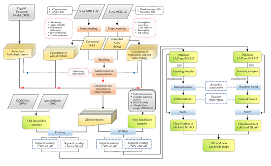
2.3. Landslide Mapping

2.3.1. Image Segmentation and Object Features

We selected subsets for the two study areas (Figure 1) that have recorded a high frequency of landslide events. A set combination of data was applied to delineate image objects using the multiresolution segmentation algorithm. We tested different scales (10, 15, 20, 25, 30, 35, 40, 45, 50, 55, and 60) and assigned the weight values of three to B11 and two for the B4, B6, B8, and B12 of Sentinel-2A and VV polarization of Sentinel-1A, as well as one to the remained bands of Sentinel-2A. To optimize segmentation, we integrated some topographic-derived indices such as slope, hillshade, terrain ruggedness index (TRI), and flow direction river (FDR) as well. The compactness and shape values were defined as 0.8 and 0.1 using the eCognition Developer 9.
We calculated a number of object features based on the statistical information of the spectral layers, contextual, geometrical, and textural characteristics of Sentinel-1A, Sentinel-2A, and their combinations. We extracted the statistics of Sentinel-2-derived vegetation, soil, and water indices for the image objects as well. These image-object features (298) were used for discriminating landslide from non-landslide objects (Table 1). In addition, about 24 topographic and hydrologic features were elicited from DEM for mapping the landslides, with the contribution of the Sentinel images (Table 1).
Table 1. Object features derived from Sentinel-1 and -2A as well as digital elevation model (DEM) for landslide mapping in NE, Iran.
TypeFeaturesStatisticsFeature Source (No.)
S11S22S1S2D3
VV Polarization and spectral layersVV, B 4, G 5, R 6, RE1 7, RE2 8, RE3 9, NNI 10, SWIR1, SWR2Mean, StdDev., pixel ratio, brightness, max diff.3275-
Spectral indicesVegetation 11: NDVI, DVI, RVI, PVI, IPVI, WDVI, TNDVI, GNDVI, GEMI, ARVI, NDI45, MTCI, REIP, S2REP, IRECI, PSSRa, MCARI, EVI2Mean, StdDev.-36--
Soil 12: SAVI, TSAVI, MSAVI, MSAVI2, BI, BI2, RI, CI-16--
Water 13: NDWI, NDWI2, MNDWI, NDPI, NDTI-10--
GeometryExtent
Shape
Area, length/width, shape index, roundness, compactness, main direction, density, asymmetry--8-
ContextualMean diff. to neighborsVV, B, G, R, RE1, RE2, RE3, NNI, SWIR1, SWR2, NDVI, EVI2, BI191-
TexturalGLCM 14 all direction (asymmetry, angular 2nd moment, correlation, contrast, dissimilarity, energy, entropy, homogeneity, maximum probability, mean, StdDev.)VV, B, G, R, RE1, RE2, RE3, NNI, SWIR1, SWR2, NDVI, EVI2, BI, NDWI2, elevation, slope, TRI, FDR 15, TWI11117945
TopographyElevation, hillshade, slope, aspect, curvature, plan curvature, profile curvature, TCI 16, TPI 17, TRI 18Mean, StdDev.---20
HydrologyFDR, TWI 19Mean, StdDev.---4
1 S1: Sentinel- 1A, 2 S2: Sentinel- 2A, 3 D: DEM; 4 B: blue, 5 G2: green, 6 R: red, 7 RE1: red-edge 1, 8 RE2: red-edge 2, 9 RE3: red-edge 3, 10 NNI: Narrow-near infrared, 11 NDVI: Normalized difference vegetation index [70], DVI: Difference vegetation index [71], RVI: Ratio vegetation index [72], PVI: Perpendicular vegetation index [73], IPVI: Infrared percentage vegetation index [74], WDVI: Weighted difference vegetation index [73,75], TNDVI: Transformed normalized difference vegetation index [76], GNDVI: Green normalized difference vegetation index [77], GEMI: Global environment monitoring index [78], ARVI: Atmospherically resistant vegetation index [79], NDI45: Normalized difference index 45 [80], MTCI: Meris terrestrial chlorophyll index [81], REIP: Red-edge inflection point [82], S2REP: Sentinel-2 red-edge position [83], IRECI: Inverted red-edge chlorophyll index [83,84], PSSRa: Pigment specific simple ratio [85], MCARI: Modified chlorophyll absorption in reflectance index [86], EVI2: Enhanced vegetation index2 [87]), 12 SAVI: Soil adjusted vegetation index [88], TSAVI: Transformed soil adjusted vegetation index [89], MSAVI: Modified soil adjusted vegetation index [90], MSAVI2: Second modified soil adjusted vegetation index [91], BI: Brightness index [92], BI2: Second brightness index [92], RI: Redness index [93], CI: Color index [93]), 13 NDWI: Normalized difference water index [94], NDWI2: Normalized difference water index 2 [95], MNDWI: Modified normalized difference water index [96], NDPI: Normalized difference pond index [97], NDTI: Normalized difference turbidity index [97]), 14 GLCM: Gray-level co-occurrence matrix [98],15 FDR: Flow direction, 16 TCI: Terrain convergence index [99], 17 TPI: Topographic position index [100],18 TRI: Terrain ruggedness index [101], 19 TWI: Topographic wetness index [102].

2.3.2. Classification by Random Forest

The random forest (RF) algorithm was applied to indicate the influential features for mapping landslides depending on the learning objects, and classifying them into the landslide-affected objects (LAO) and non-landslide-affected objects (NLAO). We used logistic regression binary analysis to obtain a reliable model that includes all object features [103]. RF builds numerous decision trees from the several random subsamples of the learning samples, and applies averaging to avoid overfitting and to increase the accuracy of the classification [54]. Approximately 20% of the objects from both the LAO and NLAO were randomly chosen for modeling. Two-thirds of the objects were assigned as learning samples (in-bag samples) of the trees, and one-third were assigned as testing samples —out of bag (OOB)— for assessing the performance of classification of the RF model [54,103]. We defined the number of trees to be built (Ntree) by 500 and 1000 for the protected and non-protected areas; the optimal trees at each node (Mtry) was determined depending on the square root of the total number of object features [104]. The variable importance (VI) was determined using the error type of the mean decrease in accuracy (MDA), which measures the difference between the (OOB) error of the outputs and the OOB error of the testing samples [54]. The performance of classification for LAO and NLAO was tested with respect to the confusion matrix using the metrics of specificity, sensitivity, precision, Kappa, negative average LogLikelihood (Neg.Av.LL), and the receiver operating characteristic (ROC) [105,106] for the two study forests. We scored entire objects based on the optimal predicted model for determining the responses of each object to the landslide hazard, and for mapping landslide-affected and non-landslide-affected objects for the protected and non-protected forests.

3. Results

3.1. Landslide Mapping

We found the optimal segmentation scale of 35 during the trial-and-error attempts from a combination set of spectral layers and topographic indices, with the optimal compactness and shape values of 0.8 and 0.1 for the two study areas. We achieved the highest performance of random forest after the formation of 500 and 1000 trees, for discriminating landslide from non-landslide objects in the protected and non-protected forests, respectively. The results of OOB showed that the accuracy values of mapping historical landslides were obtained at 86.59% and 80.30% in the protected and non-protected forests (Table 2), respectively. Moreover, the overall accuracy of landslide and non-landslide classification were 80.91% and 76.81%, depending on the Kappa in the two study forests, respectively.
We rebuilt the random forest model with respect to the top influential variables of discriminating historical landslides in both protected and non-protected forests. The maps of landslide and non-landslide objects were created depending on these variables, as shown in Figure 4.

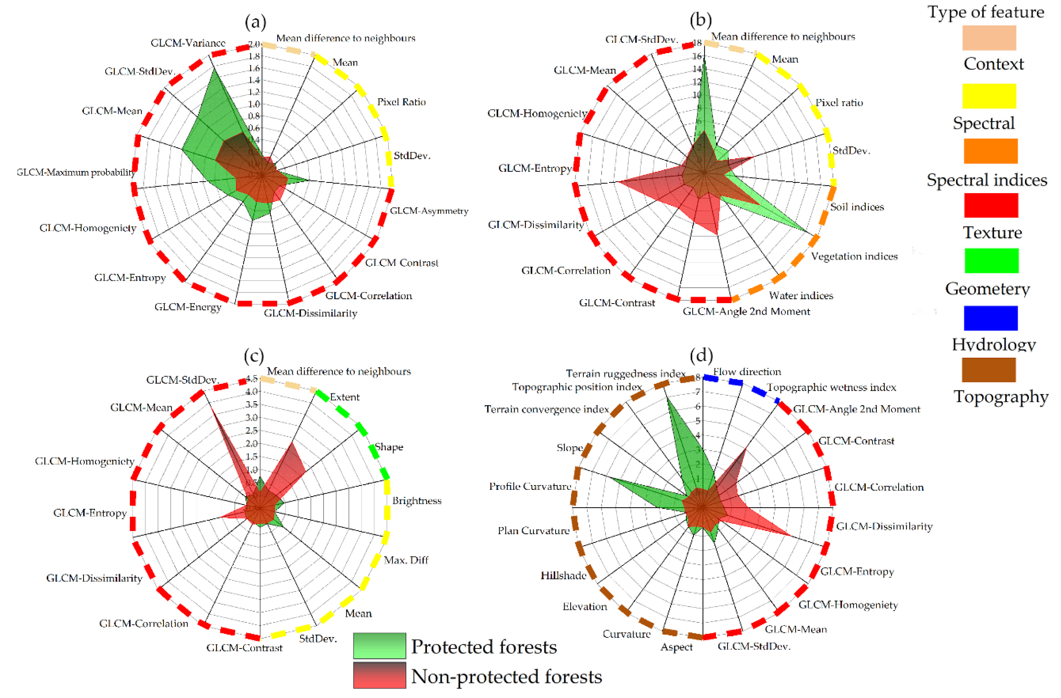
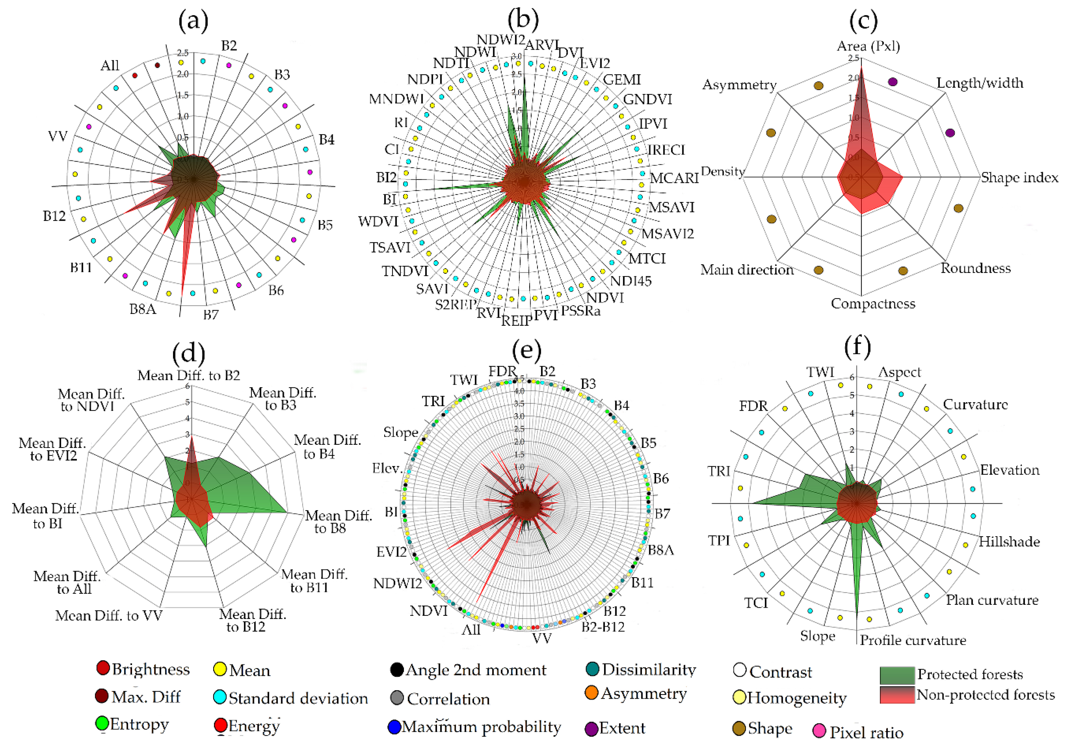
3.2. The Importance of Object Features

The results of RF indicated that the object features of Sentinel-2A and DEM have obtained the highest importance values for mapping landslides, by total importance values of 55.6% and 32% in the protected forests (old landslides), and 65.4% and 21% in the non-protected forests (new landslides), respectively. The features of Sentinel-1 and -2A recorded higher values in the non-protected forests (10%) in comparison to the protected forests (4.4%), while the performance of Sentinel-1A in the protected forests (8%) was higher than non-protected forests (3.6%).
The textural features showed the highest importance for discriminating landslides from non-landslides among the features of Sentinel-1A for both protected (7.6%) and non-protected forests (3.9%) (Figure 5a). While the contextual features (16.1%) and spectral indices (22.7%) of Sentinel-2A performed higher than other features of this sensor for detecting old landslides in the protected forests, its textural features (41.4%) recorded the highest importance values for detecting new landslides in the non-protected forests (Figure 5b). The importance of the geometrical (4.1%) and textual (5.4%) features of Sentine1-1 and -2A was considerable in the non-protected forests; however, they did not show significant importance values in the protected forests (Figure 5c). The highest importance values of the DEM derivatives were assigned to the topographic (19.4%) and textural (16.9%) features in the protected and non-protected forests (Figure 5d), respectively.
Comparison of the sub-features’ importance (Figure 6) demonstrated that the top variables for mapping old landslides were the mean of narrow-near-infrared channel (B8A) among the spectral layers; the atmospherically resistant vegetation index (ARVI) among the spectral indices; the mean difference to B8A among the contextual features; and the mean of slope among the topographic features. However, the most important sub-features for mapping new landslides were the standard deviation derived from the GLCM of all bands of Sentinel-1 and -2A, and the contrast and dissimilarity derived from the GLCM of the normalized difference water index 2 (NDWI2) among the textural features; the mean difference to the blue channel among the contextual features; the standard deviation of the red-edge 3 channel (B7) among the spectral layers; and the area size of landslides among the geometric features.

4. Discussion

4.1. Landslide Mapping Accuracy

The accuracy of discriminating landslide-affected objects from non-landslide-affected objects was satisfactory using object-oriented random forest classification by incorporating the features of Sentinel images and DEM, in both protected and non-protected forests in NE Iran. However, the performance of classification in the protected forests under the domination of old landslides was higher than in the non-protected forests under the domination of new landslides (Table 2). The performance of object-oriented random forest was verified for landslide mapping using optical images in the earlier studies [8,9,32] as well. Although the utilization of Sentinel-1 and -2A has been increasing for landslide mapping in recent studies, most of them are accomplished by the pixel-based techniques either through Sentinel-1 [1,2,42,43,44,45,47], Sentinel-2 [3,41,49], or a combination of them [4,50].

4.2. The Importance of Object Features for Mapping Old Landslides

Our analyses indicated that the spectral features of Sentinel-2A have recorded the highest importance values for discriminating old landslides in the protected forests by a total score of 33% (i.e., spectral indices: 22.7%; the first-order statistics of spectral bands: 10.3%) (Figure 5b). The textural (25.5%), topographic (19.4%), and contextual (17%) features obtained considerable scores as well, while the hydrologic (4.6%) and geometrical (<1%) features have obtained lower scores for mapping historical landslides in the protected forests (Figure 5b). These results confirm that a combination of spectral indices, topographic, textural, and contextual features are required for detecting old landslides from the background.
Slope and TRI were among the top five influential variables for mapping old landslides. The slopes above 30° (Figure 7a) contain approximately 47%, and the TRI above 14 (Figure 7c) contain 35% of the extracted landslides using the random forest model in the protected forests.
The image features that can create higher contrast between landslide-removed vegetation and their undisturbed neighbors have gained higher scores for discriminating landslide objects from non-landslide objects [8,9,10] in the protected forests. For example, the contextual feature of “mean difference to neighbors” of Sentinel-2A (Figure 7b) has gained the importance of about 16%, and the Sentinel-2-derived vegetation indices have gained a total value of 16.3% for detecting old landslides (Figure 5b). Likewise, other studies confirmed the importance of the mean difference to neighbors for detecting landslides using other satellite data [11,12,23]. Figure 6d confirmed that the mean difference to B8 showed the highest importance for mapping landslides in the protected forests. The performance of the mean difference to red or infrared bands has been highlighted for mapping landslides in the studies of Dou et al. [12] and Aksoy and Ercanoglu et al [15]. The higher scores of the textural features were recorded for those statistics derived from GLCM-Sentinel-1A that contain the dispersion of objects, such as standard deviation (Figure 5a). The use of the textural features of VV polarization of Sentinel-1A has not yet been applied for landslide mapping; however, the textural features derived from the GLCM of the multi-polarized SAR have shown high performance in mapping landslides using a multi-classifier decision [25] as well.

4.3. The Importance of Object Features for Mapping New Landslides

In contrast, in the non-protected forests, the top variables are the textural features of Sentinel-2A, combined Sentinel-1 and -2A, and Sentinel-1A for mapping the new landslides, with a total importance value of 67% (Figure 5a–c). The spectral features were recorded, with a total value of 20% (i.e., spectral indices: 11%; the first-order statistics of spectral bands: 9%), whereas the contextual, geometrical, and topographic features have shown the same importance of about 4% (Figure 5). The influential variables of the textural features for mapping new landslides are GLCM-Entropy [9,23,28], GLCM-Angle 2nd moment [12,28], GLCM-Dissimilarity [12], and GLCM-Correlation [9,23,28] of Sentinel-2A, along with the GLCM-StDev [9,12,30] of Sentinel-1 and -2A in the non-protected forests (Figure 5b,c). The highest importance, among the textural features, was assigned to the standard deviation derived from the GLCM of all channels of Sentinel-1 and -2A (Figure 8a) for the mapping new landslides (Figure 6e). The other top variables were the contrast derived from the GLCM of NDWI2 (Figure 8b), the mean difference to neighbors of the blue band (Figure 8c), the dissimilarity derived from the GLCM of NDWI2 (Figure 8d), and the standard deviation values of the red-edge 3 band (Figure 8e). Nevertheless, some earlier researchers reported the superiority of other derived features from the GLCM such as homogeneity, density, mean, and the contrast of other satellite images for landslide mapping [6].
Although the topographic features derived from the DEM, such as TRI [41] and slope [9,10,13], were the top variables for mapping old landslides (Figure 6f and Figure 7a,c), the textural features derived from the DEM, such as GLCM-Angle 2nd moment and GLCM-Entropy [27], were the important variables for mapping new landslides in the non-protected forests (Figure 5d). The integration of textural-derived features from the DEM, such as GLCM-features [24,26], was recommended to increase the accuracy of landslide mapping in the earlier studies [26]. Hervás and Rosin [24] concluded that the features derived from the GLCM of topography facilitate landslide mapping, through differentiating between coarse and smoothed surfaces, or dense forest-stands and landslide-opened forests. Although the Sentinel-2-derived vegetation indices such as the ARVI, GNDVI, TNDVI, and NDVI gained high importance values, some soil and water indices such as the BI2 and NDWI2 were recorded with high scores for mapping landslides in the protected forests (Figure 6b) as well.
The vegetation indices are useful for discriminating landslide-induced barren lands, debris flows, and failure slopes from surrounding undisturbed-forest areas [10,16,18,20]. The improvement of landslide detection from different optical sensors by the incorporating vegetation indices like NDVI derived from ETM+ [14,15], SPOT-5 [17], and GF-1 [10]; GNDVI derived from SPOT-5 [17] and Resourcesat-2 LISS-IV [20]; and TNDVI derived from IRS-P6 LISS-IV [22], was reported in different research. However, our results emphasize on the application of some Sentinel-2-based soil and water indices for mapping landslides as well. While soil brightness indices were proposed [16] for detecting landslide-disturbed vegetation, and NDWI for detecting landslide-opened water bodies [6,19,21], the adjusted BI and NDWI (i.e., BI2 and NDWI2) derived from Sentinel-2A were superior for mapping landslides in this study. Moreover, this study suggests a high performance of some vegetation indices that are less sensitive to the atmospheric effects, such as the ARVI and PVI for landslide mapping in forest areas.
The final models of random forest were rebuilt, based on the top variables that at least have obtained an importance value of above one percent (Figure 9). Figure 9a shows that the statistics of topography, hydrology, Sentinel-2 bands, and their ratios are dominating in the formation of the new trained model for mapping historical landslides in the protected forests. On the other hand, Figure 9b confirmed that textural features derived from the GLCM of the combination of Sentinel-1 and -2A, and Sentinel-2A and topography, were influential variables of forming the new trained model for mapping landslides in the non-protected forests.
This study has utilized object features derived from different bands of Sentinel-2A and VV polarization of Sentinel-1A for detecting historical landslide from non-landslide objects. Nevertheless, we had limitations about the availability of dual polarimetry products of Sentinel-1 such as VV-VH or HH-HV, due to synchronization with the Sentinel-2 in the study area, for increasing detection of hidden landslides by regenerated vegetation [25]. We also suggest the integration of Sentinel images with the other radar data, which are acquired in the L spectrum, for penetrating dense forest cover and mapping possible landslide events. Moreover, some new landslide events might be caused by human activities, such as forest conversion to farmlands, forest harvesting, road building, and mining in the non-protected forest, which need to be carefully considered for mapping historical landslides by the future studies.

5. Conclusions

This study has developed a new analysis for mapping historical landslides with the contributions of Sentinel-1A, Sentinel-2A, and DEM derivatives using the object-oriented random forest approach in the protected and non-protected forests in NE Iran.
The use of hundreds of derived features from Sentinel images and topographic data revealed that the influential variables for detecting historical landslides in the protected and non-protected forests are different. The top influential features for mapping old landslides are Sentinel-2-derived indices, contextual features, and topographic layers in the protected forests. However, the textural features of Sentinel-2A, Sentinel-1 and -2A, and topographic variables gained higher importance for mapping new landslides in the non-protected forests.
The high mean values of the slope, TRI, and the difference to the neighbors of the narrow-near infrared and red bands of Sentinel-2 significantly differentiated historical landslides from non-landslides in the protected forests. However, the standard deviation derived from the GLCM of all channels (Sentinel-1 and -2A), and the contrast and dissimilarity derived from the GLCM of NDWI2 were the top influential sub-features for mapping new landslides in the non-protected forests. Furthermore, the high importance of other object features can be considered for mapping historical landslides such as ARVI, GNDVI, BI2, and the standard deviation derived from the GLCM of VV polarization in the protected forests, and the mean difference to neighbors of B2 and the flow direction river in the non-protected forests. These findings highlight that a synergetic of Sentinel- and DEM-derived features needs to be employed for mapping historical landslides in the forest regions.
This study suggests testing the ability of the dual polarization of Sentinel-1 (VV-VH, or HH-HV) with the combination of Sentinel-2, for the mapping of landslides in forest areas. We compared the importance of common features for mapping historical landslides in the protected and non-protected forests; however, exerting some human-induced features such as deforestation, forest fragmentation induced by developing infrastructures, and logging and mining activities, may facilitate landslide detection in the non-protected forests as well.
We have proposed an object-oriented framework to discern historical landslides from the forest background, with the contributions of freely available Sentinel images and ancillary data. The result can be applied for the real-time assessing of landslide-caused disasters, the identifying of the spatiotemporal patterns of landslide events (for forest managers and engineers), and the analyzing of the susceptibility of forests to landslide hazards.

Author Contributions

Z.S. contributed to the design, image analysis using SNAP and eCognition®, and in writing the manuscript; O.A. and Z.S. made contributions to the statistical analyses in R, and O.A. designed graphs; M.B. reviewed the manuscript and supervised at all stages of the study. All authors read and approved the submitted manuscript.

Funding

This research received no external funding.

Acknowledgments

This study is a part of the first author’s doctoral dissertation under the supervision of the third author. The author acknowledges support by the German Research Foundation and the Open Access Funding by the Publication Fund of the TU Dresden. Authors would like to thank the anonymous reviewers whose comments have greatly improved this manuscript.

Conflicts of Interest

The authors declare no conflict of interest.

Appendix A

Table A1. Main characteristics of Sentinel-1A image.
Characteristics
BandC-band
WavelengthC-band (3.75–7.5 cm)
Product typeGround Range Detected (GRD)
Polarization Single (VV)
Orbit typeAscending
Pixel spacing 10 × 10 m (range × azimuth)
Incidence angle (˚)30.6–46.0
Table A2. The characteristics of the Sentinel-2 satellite.
BandSpatial ResolutionSpectral Resolution
B1 Aerosol Ultra blue60 m433–453 nm
B2 Blue10 m458–523 nm
B3 Green10 m543–578 nm
B4 Red10 m650–680 nm
B5 Red-edge 1 Visible and Near Infrared20 m698–713 nm
B6 Red-edge 2 Visible and Near Infrared20 m733–748 nm
B7 Red-edge 3 Visible and Near Infrared20 m765–785 nm
B8 Wide near infrared wide10 m785–900 nm
B8A Narrow near infrared20 m855–875 nm
B9 Cloud60 m930–950 nm
B10 Water vapor SWIR60 m1365–1358 nm
B11 SWIR1 Short Wave Infrared20 m1565–1655 nm
B12 SWIR2 Short Wave Infrared20 m2100–2280 nm

References

  1. Barra, A.; Solari, L.; Béjar-Pizarro, M.; Monserrat, O.; Bianchini, S.; Herrera, G.; Crosetto, M.; Sarro, R.; González-Alonso, E.; Mateos, R. A methodology to detect and update active deformation areas based on sentinel-1 SAR images. Remote Sens. 2017, 9, 1002. [Google Scholar] [CrossRef]
  2. Solari, L.; Del Soldato, M.; Montalti, R.; Bianchini, S.; Raspini, F.; Thuegaz, P.; Bertolo, D.; Tofani, V.; Casagli, N. A Sentinel-1 based hot-spot analysis: Landslide mapping in north-western Italy. Int. J. Remote Sens. 2019, 40, 7898–7921. [Google Scholar] [CrossRef]
  3. Qin, Y.; Lu, P.; Li, Z. Landslide inventory mapping from bitemporal 10 m Sentinel-2 images using change detection based Markov Random Field. Int. Arch. Photogramm. Remote Sens. Spat. Inf. Sci. 2018, 42, 1447–1452. [Google Scholar] [CrossRef]
  4. Jelének, J.; Kopačková, V.; Fárová, K. Post-earthquake landslide distribution assessment using sentinel-1 and -2 data: The example of the 2016 mw 7.8 earthquake in New Zealand. Proceedings 2018, 2, 361. [Google Scholar] [CrossRef]
  5. Veblen, T.T.; Ashton, D.H. Catastrophic influences on the vegetation of the Valdivian Andes, Chile. Vegetatio 1978, 36, 149–167. [Google Scholar] [CrossRef]
  6. Cao, W.; Tong, X.H.; Liu, S.C.; Wang, D. Landslides extraction from diverse remote sensing data sources using semantic reasoning scheme. Int. Arch. Photogramm. Remote Sens. Spatial Inf. Sci. 2016, XLI-B8, 25–31. [Google Scholar] [CrossRef]
  7. Zhao, C.; Lu, Z. Remote sensing of landslides—A review. Remote Sens. 2018, 10, 279. [Google Scholar] [CrossRef]
  8. Stumpf, A.; Kerle, N. Combining Random Forests and object-oriented analysis for landslide mapping from very high resolution imagery. Procedia Environ. Sci. 2011, 3, 123–129. [Google Scholar] [CrossRef] [Green Version]
  9. Stumpf, A.; Kerle, N. Object-oriented mapping of landslides using Random Forests. Remote Sens. Environ. 2011, 115, 2564–2577. [Google Scholar] [CrossRef]
  10. Sun, W.; Tian, Y.; Mu, X.; Zhai, J.; Gao, P.; Zhao, G. Loess landslide inventory map based on GF-1 satellite imagery. Remote Sens. 2017, 9, 314. [Google Scholar] [CrossRef]
  11. Martha, T.R.; Kerle, N.; Jetten, V.; van Westen, C.J.; Kumar, K.V. Characterising spectral, spatial and morphometric properties of landslides for semi-automatic detection using object-oriented methods. Geomorphology 2010, 116, 24–36. [Google Scholar] [CrossRef]
  12. Dou, J.; Chang, K.-T.; Chen, S.; Yunus, A.; Liu, J.-K.; Xia, H.; Zhu, Z. Automatic case-based reasoning approach for landslide detection: Integration of object-oriented image analysis and a genetic algorithm. Remote Sens. 2015, 7, 4318–4342. [Google Scholar] [CrossRef]
  13. Hölbling, D.; Betts, H.; Spiekermann, R.; Phillips, C. Identifying spatio-temporal landslide hotspots on north island, New Zealand, by analyzing historical and recent aerial photography. Geosciences 2016, 6, 48. [Google Scholar] [CrossRef]
  14. Barlow, J.; Martin, Y.; Franklin, S.E. Detecting translational landslide scars using segmentation of Landsat ETM+ and DEM data in the northern Cascade Mountains, British Columbia. Can. J. Remote Sens. 2003, 29, 510–517. [Google Scholar] [CrossRef]
  15. Aksoy, B.; Ercanoglu, M. Landslide identification and classification by object-based image analysis and fuzzy logic: An example from the Azdavay region (Kastamonu, Turkey). Comput. Geosci. 2012, 38, 87–98. [Google Scholar] [CrossRef]
  16. Yang, S.; Li, Y.; Feng, G.; Zhang, L. A method aimed at automatic landslide extraction based on background values of satellite imagery. Int. J. Remote Sens. 2014, 35, 2247–2266. [Google Scholar]
  17. Hölbling, D.; Friedl, B.; Eisank, C. An object-based approach for semi-automated landslide change detection and attribution of changes to landslide classes in northern Taiwan. Earth Sci. Inform. 2015, 8, 327–335. [Google Scholar] [CrossRef] [Green Version]
  18. Casagli, N.; Cigna, F.; Bianchini, S.; Hölbling, D.; Füreder, P.; Righini, G.; Del Conte, S.; Friedl, B.; Schneiderbauer, S.; Iasio, C.; et al. Landslide mapping and monitoring by using radar and optical remote sensing: Examples from the EC-FP7 project SAFER. Remote Sens. Appl. Soc. Environ. 2016, 4, 92–108. [Google Scholar] [CrossRef] [Green Version]
  19. Ding, A.; Zhang, Q.; Zhou, X.; Dai, B. Automatic recognition of landslide based on CNN and texture change detection. In Proceedings of the 31st Youth Academic Annual Conference of Chinese Association of Automation, Wuhan, China, 11–13 November 2016; IEEE: Piscataway, NJ, USA, 2016; pp. 444–448. [Google Scholar]
  20. Veena, V.S.; Sai, S.G.; Tapas, R.M.; Deepak, M.; Rama, R.N. Automatic detection of landslides in object-based environment using open source tools. In Proceedings of the GEOBIA 2016, Solutions and synergies, Enschede, The Netherlands, 14–16 September 2016. [Google Scholar] [CrossRef]
  21. Le, T.T.T.; Kawagoe, S. Landslide detection analysis in North Vietnam base on satellite images and digital geographical Information-Landsat 8 satellite and historical data Approaches. J. JSCE Ser. G 2017, 73. [Google Scholar] [CrossRef]
  22. Sengar, S.S.; Ghosh, S.K.; Kumar, A.; Chaudhary, H. Landslide identification from IRS-P6 LISS-IV temporal data-a comparative study using fuzzy based classifiers. Int. Arch. Photogramm. Remote Sens. Spat. Inf. Sci. 2018, XLII-3/W4, 461–467. [Google Scholar] [CrossRef]
  23. Moine, M.; Puissant, A.; Malet, J.P. Detection of landslides from aerial and satellite images with a semi-automatic method. Application to the Barcelonnette Basin (Alps-de-Haute-Provence). In Landslide Processes: From Geomorphological Mapping to Dynamic Modelling; Malet, J.-P., Remaitre, A., Bogaard, T., Eds.; CERG: Strasbourg, France, 2009; pp. 63–68. [Google Scholar]
  24. Hervás, J.; Rosin, P.L. Landslide mapping by textural analysis of ATM data. In Proceedings of the Eleventh Thematic Conference and Workshops on Applied Geologic Remote Sensing, Las Vegas, NV, USA, 27–29 February 1996; pp. II394–II402. [Google Scholar]
  25. Cui, M.; Prasad, S.; Mahrooghy, M.; Aanstoos, J.V.; Lee, M.A.; Bruce, L.M. Decision fusion of textural features derived from polarimetric data for Levee assessment. IEEE J. Sel. Top. Appl. Earth Obs. Remote Sens. 2012, 5, 970–976. [Google Scholar] [CrossRef]
  26. Blaschke, T.; Feizizadeh, B.; Holbling, D. Object-based image analysis and digital terrain analysis for locating landslides in the Urmia Lake Basin, Iran. IEEE J. Sel. Top. Appl. Earth Obs. Remote Sens. 2014, 7, 4806–4817. [Google Scholar] [CrossRef]
  27. Chen, W.; Li, X.; Wang, Y.; Chen, G.; Liu, S. Forested landslide detection using LiDAR data and the random forest algorithm: A case study of the Three Gorges, China. Remote Sens. Environ. 2014, 152, 291–301. [Google Scholar] [CrossRef]
  28. Li, X.; Cheng, X.; Chen, W.; Chen, G.; Liu, S. Identification of forested landslides using LiDar data, object-based image analysis, and machine learning algorithms. Remote Sens. 2015, 7, 9705–9726. [Google Scholar] [CrossRef]
  29. Feizizadeh, B.; Blaschke, T.; Tiede, D.; Moghaddam, M.H.R. Evaluating fuzzy operators of an object-based image analysis for detecting landslides and their changes. Geomorphology 2017, 293, 240–254. [Google Scholar] [CrossRef]
  30. Attarzadeh, R.; Amini, J.; Notarnicola, C.; Greifeneder, F. Synergetic use of Sentinel-1 and Sentinel-2 data for soil moisture mapping at plot scale. Remote Sens. 2018, 10, 1285. [Google Scholar] [CrossRef]
  31. Barlow, J.; Franklin, S.; Martin, Y. High spatial resolution satellite imagery, DEM derivatives, and image segmentation for the detection of mass wasting processes. Photogramm. Eng. Remote Sens. 2006, 72, 687–692. [Google Scholar] [CrossRef]
  32. Stumpf, A.; Lachiche, N.; Kerle, N.; Malet, J.P.; Puissant, A. Adaptive spatial sampling with active random forest for object-oriented landslide mapping. In Proceedings of the 2012 IEEE International Geoscience and Remote Sensing Symposium, Munich, Germany, 22–27 July 2012. [Google Scholar]
  33. Martha, T.R.; Kerle, N.; Van Westen, C.J.; Jetten, V.; Vinod Kumar, K. Object-oriented analysis of multi-temporal panchromatic images for creation of historical landslide inventories. ISPRS J. Photogramm. Remote Sens. 2012, 67, 105–119. [Google Scholar] [CrossRef]
  34. Colesanti, C.; Wasowski, J. Investigating landslides with space-borne Synthetic Aperture Radar (SAR) interferometry. Eng. Geo. 2006, 88, 173–199. [Google Scholar] [CrossRef]
  35. Notti, D.; Davalillo, J.C.; Herrera, G.; Mora, O. Assessment of the performance of X-band satellite radar data for landslide mapping and monitoring: Upper Tena Valley case study. Nat. Hazards Earth Syst. Sci. 2010, 10, 1865–1875. [Google Scholar] [CrossRef]
  36. Raspini, F.; Ciampalini, A.; Del Conte, S.; Lombardi, L.; Nocentini, M.; Gigli, G.; Ferretti, A.; Casagli, N. Exploitation of amplitude and phase of satellite SAR images for landslide mapping: The case of Montescaglioso (South Italy). Remote Sens. 2015, 7, 14576–14596. [Google Scholar] [CrossRef]
  37. Mondini, A. Measures of spatial autocorrelation changes in multitemporal SAR images for event landslides detection. Remote Sens. 2017, 9, 554. [Google Scholar] [CrossRef]
  38. Delacourt, C.; Raucoules, D.; Le Mouélic, S.; Carnec, C.; Feurer, D.; Allemand, P.; Cruchet, M. Observation of a large landslide on La Reunion Island using differential SAR interferometry (JERS and Radarsat) and correlation of optical (Spot5 and Aerial) images. Sensors 2009, 9, 616–630. [Google Scholar] [CrossRef] [PubMed]
  39. Plank, S.; Twele, A.; Martinis, S. Landslide mapping in vegetated areas using change detection based on optical and polarimetric SAR data. Remote Sens. 2016, 8, 307. [Google Scholar] [CrossRef]
  40. Plank, S.; Hölbling, D.; Eisank, C.; Friedl, B.; Martinis, S.; Twele, A. Comparing object-based landslide detection methods based on polarimetric SAR and optical satellite imagery—A case study in Taiwan. In Proceedings of the 7th International Workshop on Science and Applications of SAR Polarimetry and Polarimetric Interferometry, POLinSAR 2015, Frascati, Italy, 27–30 January 2015; pp. 27–30. [Google Scholar]
  41. Hölbling, D.; Eisank, C.; Albrecht, F.; Vecchiotti, F.; Friedl, B.; Weinke, E.; Kociu, A. Comparing manual and semi-automated landslide mapping based on optical satellite images from different sensors. Geosciences 2017, 7, 37. [Google Scholar] [CrossRef]
  42. Barra, A.; Monserrat, O.; Mazzanti, P.; Esposito, C.; Crosetto, M.; Scarascia, G. Potentiality of SENTINEL-1 for landslide detection: First results in the Molise Region (Italy). In Proceedings of the European Geosciences Union General Assembly; Geophysical Research Abstracts; Vol. 18, EGU2016–2916, Vienna, Austria, 17–22 April 2016. [Google Scholar]
  43. Barra, A.; Monserrat, O.; Mazzanti, P.; Esposito, C.; Crosetto, M.; Scarascia Mugnozza, G. First insights on the potential of Sentinel-1 for landslides detection. Geomat. Nat. Hazards Risk 2016, 7, 1874–1883. [Google Scholar] [CrossRef] [Green Version]
  44. Barra, A.; Monserrat, O.; Crosetto, M.; Cuevas-Gonzalez, M.; Devanthéry, N.; Luzi, G.; Crippa, B. Sentinel-1 Data Analysis for Landslide Detection and Mapping: First Experiences in Italy and Spain. In 2017—Advancing Culture of Living; Mikoš, A., Ed.; Springer International Publishing: Cham, Switzerland, 2017; pp. 201–208. [Google Scholar] [Green Version]
  45. Fiaschi, S.; Mantovani, M.; Frigerio, S.; Pasuto, A.; Floris, M. Testing the potential of Sentinel-1A TOPS interferometry for the detection and monitoring of landslides at local scale (Veneto Region, Italy). Environ. Earth Sci. 2017, 76, 1874. [Google Scholar] [CrossRef]
  46. Kovács, I.P.; Bugya, T.; Czigány, S.; Defilippi, M.; Lóczy, D.; Riccardi, P.; Ronczyk, L.; Pasquali, P. How to avoid false interpretations of Sentinel-1A TOPSAR interferometric data in landslide mapping? A case study: Recent landslides in Transdanubia, Hungary. Nat. Hazards 2019, 96, 693–712. [Google Scholar] [CrossRef]
  47. Kyriou, A.; Nikolakopoulos, K. Assessing the suitability of Sentinel-1 data for landslide mapping. Eur. J. Remote Sens. 2018, 51, 402–411. [Google Scholar] [CrossRef] [Green Version]
  48. Mondini, A.; Santangelo, M.; Rocchetti, M.; Rossetto, E.; Manconi, A.; Monserrat, O. Sentinel-1 SAR amplitude imagery for rapid landslide detection. Remote Sens. 2019, 11, 760. [Google Scholar] [CrossRef]
  49. Stumpf, A.; Marc, O.; Malet, J.; Michea, D. Sentinel-2 for rapid operational landslide inventory mapping. In Proceedings of the 19th EGU General Assembly; Geophysical Research Abstracts, Vol. 19, EGU2017–4449, Vienna, Austria, 23–28 April 2017. [Google Scholar]
  50. Kyriou, A.; Nikolakopoulos, K.G. A synergy of radar and optical data of Copernicus programme for landslide mapping. In Proceedings of the Earth Resources and Environmental Remote Sens./GIS Applications IX, Berlin, Germany, 10–13 September 2018; Michel, U., Schulz, K., Eds.; SPIE: Bellingham, WA, USA, 2018; Volume 10790, pp. 107900G-1–107900G-10. [Google Scholar] [CrossRef]
  51. Chen, T.; Trinder, J.; Niu, R. Object-Oriented landslide mapping using ZY-3 satellite imagery, Random Forest and mathematical morphology, for the Three-Gorges Reservoir, China. Remote Sens. 2017, 9, 333. [Google Scholar] [CrossRef]
  52. Mayr, A.; Rutzinger, M.; Bremer, M.; Oude Elberink, S.; Stumpf, F.; Geitner, C. Object-based classification of terrestrial laser scanning point clouds for landslide monitoring. Photogramm. Rec. 2017, 32, 377–397. [Google Scholar] [CrossRef] [Green Version]
  53. Park, N.-W.; Chi, K.-H. Quantitative assessment of landslide susceptibility using high-resolution remote sensing data and a generalized additive model. Int. J. Remote Sens. 2008, 29, 247–264. [Google Scholar] [CrossRef]
  54. Breiman, L. Random Forests. Mach. Learn. 2001, 45, 5–32. [Google Scholar] [CrossRef] [Green Version]
  55. Körting, T.S.; Garcia Fonseca, L.M.; Câmara, G. GeoDMA—Geographic data mining analyst. Comput. Geosci. 2013, 57, 133–145. [Google Scholar] [CrossRef]
  56. Belgiu, M.; Drăguţ, L. Random forest in remote sensing: A review of applications and future directions. ISPRS J. Photogramm. Remote Sens. 2016, 114, 24–31. [Google Scholar] [CrossRef]
  57. Salford Systems Ltd. Salford Predictive Modeller: Introduction to Random Forests. Available online: https://www.salford-systems.com/support/spm-user-guide/help/randomforests (accessed on 2 October 2019).
  58. Pradhan, B.; Alsaleh, A. A supervised object-based detection of landslides and man-made slopes using airborne laser scanning data. In Laser Scanning Applications in Landslide Assessment; Pradhan, B., Ed.; Springer International Publishing: Cham, Germany, 2017; pp. 23–50. [Google Scholar]
  59. Pradhan, B.; Mezaal, M.R. Optimized rule sets for automatic landslide characteristic detection in a highly vegetated forests. In Laser Scanning Applications in Landslide Assessment; Pradhan, B., Ed.; Springer International Publishing: Cham, Germany, 2017; pp. 51–68. [Google Scholar]
  60. Pradhan, B.; Seeni, M.I.; Nampak, H. Integration of LiDAR and QuickBird data for automatic landslide detection using object-based analysis and random forests. In Laser Scanning Applications in Landslide Assessment; Springer: Cham, The Netherlands, 2017; pp. 69–81. [Google Scholar]
  61. Mezaal, M.; Pradhan, B.; Rizeei, H. Improving landslide detection from airborne laser scanning data using optimized Dempster–Shafer. Remote Sens. 2018, 10, 1029. [Google Scholar] [CrossRef]
  62. Sagheb Talebi, K.; Sajedi, T.; Pourhashemi, M. Forests of Iran; Springer: Dordrecht, The Netherlands, 2014. [Google Scholar]
  63. Abdi, O.; Shirvani, Z.; Buchroithner, M.F. Spatiotemporal drought evaluation of Hyrcanian deciduous forests and semi-steppe rangelands using moderate resolution imaging spectroradiometer time series in Northeast Iran. Land Degrad. Develop. 2018, 29, 2525–2541. [Google Scholar] [CrossRef]
  64. Abdi, O.; Shirvani, Z.; Buchroithner, M.F. Forest drought-induced diversity of Hyrcanian individual-tree mortality affected by meteorological and hydrological droughts by analyzing moderate resolution imaging spectroradiometer products and spatial autoregressive models over northeast Iran. Agric. For. Meteorol. 2019, 275, 265–276. [Google Scholar] [CrossRef]
  65. Abdi, O.; Kamkar, B.; Shirvani, Z.; Teixeira da Silva, J.A.; Buchroithner, M.F. Spatial-statistical analysis of factors determining forest fires: A case study from Golestan, Northeast Iran. Geomat. Nat. Hazards Risk 2018, 9, 267–280. [Google Scholar] [CrossRef]
  66. Abdi, O. Climate-Triggered Insect Defoliators and Forest Fires Using Multitemporal Landsat and TerraClimate Data in NE Iran: An Application of GEOBIA TreeNet and Panel Data Analysis. Sensors 2019, 19, 3965. [Google Scholar] [CrossRef] [PubMed]
  67. Shirvani, Z.; Abdi, O.; Buchroithner, M.F.; Pradhan, B. Analysing spatial and statistical dependencies of deforestation affected by residential growth: Gorganrood basin, Northeast Iran. Land Degrad. Develop. 2017, 28, 2176–2190. [Google Scholar] [CrossRef]
  68. Iranian Landslide Working Party (ILWP). Iranian Landslides List; Forest, Rangeland and Watershed Association: Tehran, Iran, 2007; 60p. [Google Scholar]
  69. Filipponi, F. Sentinel-1 GRD Preprocessing Workflow. Proceedings 2019, 18, 11. [Google Scholar] [CrossRef]
  70. Rouse Jr, J.; Haas, R.H.; Schell, J.A.; Deering, D.W. Monitoring vegetation systems in the Great Plains with ERTS. Nasa Spec. Publ. 1973, 351, 309. [Google Scholar]
  71. Tucker, C.J. Red and photographic infrared linear combinations for monitoring vegetation. Remote Sens. Environ. 1979, 8, 127–150. [Google Scholar] [CrossRef] [Green Version]
  72. Pearson, R.L.; Miller, L.D. Remote mapping of standing crop biomass for estimation of the productivity of the shortgrass prairie. In Proceedings of the Remote Sensing of Environment, VIII, ERIM, Ann Arbor, MI, USA, 2–6 October 1972; pp. 1355–1379. [Google Scholar]
  73. Richardson, A.J.; Wiegand, C.L. Distinguishing vegetation from soil background information. Photogramm. Eng. Remote Sens. 1977, 43, 1541–1552. [Google Scholar]
  74. Crippen, R. Calculating the vegetation index faster. Remote Sens. Environ. 1990, 34, 71–73. [Google Scholar] [CrossRef]
  75. Clevers, J. The derivation of a simplified reflectance model for the estimation of leaf area index. Remote Sens. Environ. 1988, 25, 53–69. [Google Scholar] [CrossRef]
  76. Deering, D.W.; Rouse, J.W.; Haas, R.H.; Schell, J.A. Measuring” forage production” of grazing units from Landsat MSS data. In Proceedings of the Tenth International Symposium of Remote Sensing of the Environment, ERIM, Ann Arbor, MI, USA, 23–25 August 1975; pp. 1169–1178. [Google Scholar]
  77. Gitelson, A.A.; Kaufman, Y.J.; Merzlyak, M.N. Use of a green channel in remote sensing of global vegetation from EOS-MODIS. Remote Sens. Environ. 1996, 58, 289–298. [Google Scholar] [CrossRef]
  78. Pinty, B.; Verstraete, M.M. GEMI: A non-linear index to monitor global vegetation from satellites. Vegetatio 1992, 101, 15–20. [Google Scholar] [CrossRef]
  79. Kaufman, Y.J.; Tanre, D. Atmospherically resistant vegetation index (ARVI) for EOS-MODIS. IEEE Trans. Geosci. Remote Sens. 1992, 30, 261–270. [Google Scholar] [CrossRef]
  80. Delegido, J.; Verrelst, J.; Alonso, L.; Moreno, J. Evaluation of Sentinel-2 red-edge bands for empirical estimation of green LAI and chlorophyll content. Sensors 2011, 11, 7063–7081. [Google Scholar] [CrossRef] [PubMed]
  81. Dash, J.; Curran, P.J. The MERIS terrestrial chlorophyll index. Int. J. Remote Sens. 2004, 25, 5403–5413. [Google Scholar] [CrossRef]
  82. Guyot, G.; Baret, F. Utilisation de la Haute Resolution Spectrale pour Suivre L’etat des Couverts Vegetaux. Spectr. Signat. Objects Remote Sens. 1988, 287, 279. [Google Scholar]
  83. Frampton, W.J.; Dash, J.; Watmough, G.; Milton, E.J. Evaluating the capabilities of Sentinel-2 for quantitative estimation of biophysical variables in vegetation. ISPRS J. Photogramm. Remote Sens. 2013, 82, 83–92. [Google Scholar] [CrossRef] [Green Version]
  84. Clevers, J.G.P.W.; Jong, S.M.; De Epema, G.F.; Addink, E.A. Meris and the Red-edge index. In Second 747 EARSeL Workshop Imaging Spectroscopy; EARSeL: Enschede, The Netherlands, 2000. [Google Scholar]
  85. Blackburn, G.A. Quantifying chlorophylls and caroteniods at leaf and canopy scales. Remote Sens. Environ. 1998, 66, 273–285. [Google Scholar] [CrossRef]
  86. Daughtry, C. Estimating corn leaf chlorophyll concentration from leaf and canopy reflectance. Remote Sens. Environ. 2000, 74, 229–239. [Google Scholar] [CrossRef]
  87. Jiang, Z.; Huete, A.R.; Didan, K.; Miura, T. Development of a two-band enhanced vegetation index without a blue band. Remote Sens. Environ. 2008, 112, 3833–3845. [Google Scholar] [CrossRef]
  88. Huete, A.R. A soil-adjusted vegetation index (SAVI). Remote Sens. Environ. 1988, 25, 295–309. [Google Scholar] [CrossRef]
  89. Baret, F.; Guyot, G.; Major, D.J. TSAVI: A vegetation index which minimizes soil brightness effects on LAI and APAR estimation. In Proceedings of the 12th IEEE Canadian Symposium on Remote Sensing Geoscience and Remote Sensing Symposium, Vancouver, BC, Canada, 10–14 July 1989; pp. 1355–1358. [Google Scholar]
  90. Qi, J.; Chehbouni, A.; Huete, A.R.; Kerr, Y.H.; Sorooshian, S. A modified soil adjusted vegetation index. Remote Sens. Environ. 1994, 48, 119–126. [Google Scholar] [CrossRef]
  91. Qi, J.; Kerr, Y.; Chehbouni, A. External factor consideration in vegetation index development. In Proceedings of the 6th International Symposium on Physical Measurements and Signatures in Remote Sensing, Val D’Isere, France, 17–22 January 1994; pp. 723–730. [Google Scholar]
  92. Escadafal, R. Remote sensing of arid soil surface color with Landsat thematic mapper. Adv. Space Res. 1989, 9, 159–163. [Google Scholar] [CrossRef]
  93. Pouget, M.; Madeira, J.; Le Floch, E.; Kamal, S. Caracteristiques spectrales des surfaces sableuses de la region cot&e Nord-Ouest de I’Egypte: Application aux don&es satellitaires SPOT. In Proceedings of the 2eme JoumCes de T&detection: Caracterisation et Suivi des Milieux Terrestres en Regions Arides et Tropicales, Ed. ORSTOM, Collection Colloques et Seminaires, Paris, France, 4–6 December 1990; pp. 27–38. [Google Scholar]
  94. Gao, B.-C. NDWI—A normalized difference water index for remote sensing of vegetation liquid water from space. Remote Sens. Environ. 1996, 58, 257–266. [Google Scholar] [CrossRef]
  95. McFeeters, S.K. The use of the normalized difference water index (NDWI) in the delineation of open water features. Int. J. Remote Sens. 1996, 17, 1425–1432. [Google Scholar] [CrossRef]
  96. Xu, H. Modification of normalised difference water index (NDWI) to enhance open water features in remotely sensed imagery. Int. J. Remote Sens. 2006, 27, 3025–3033. [Google Scholar] [CrossRef]
  97. Lacaux, J.P.; Tourre, Y.M.; Vignolles, C.; Ndione, J.A.; Lafaye, M. Classification of ponds from high-spatial resolution remote sensing: Application to Rift Valley Fever epidemics in Senegal. Remote Sens. Environ. 2007, 106, 66–74. [Google Scholar] [CrossRef]
  98. Haralick, R.M.; Shanmugam, K. Textural features for image classification. IEEE Trans. Syst. Man Cybern. 1973, 610–621. [Google Scholar] [CrossRef]
  99. Köthe, R.; Lehmeier, F. SARA-system zur automatischen relief-analyse. User Manual. Unpublished work. 1996. [Google Scholar]
  100. Wilson, J.P.; Gallant, J.C. Terrain Analysis: Principles and Applications; Wilson, J.P., Gallant, J.C., Eds.; John Wiley & Sons: New York, NY, USA, 2000; ISBN 0471321885. [Google Scholar]
  101. Riley, S.J.; DeGloria, S.D.; Elliot, R. Index that quantifies topographic heterogeneity. Intermt. J. Sci. 1999, 5, 23–27. [Google Scholar]
  102. Moore, I.D.; Grayson, R.B.; Ladson, A.R. Digital terrain modelling: A review of hydrological, geomorphological, and biological applications. Hydrol. Process. 1991, 5, 3–30. [Google Scholar] [CrossRef]
  103. Liaw, A.; Wiener, M. Classification and regression by randomForest. R News 2002, 2, 18–22. [Google Scholar]
  104. Gislason, P.O.; Benediktsson, J.A.; Sveinsson, J.R. Random forests for land cover classification. Pattern Recognit. Lett. 2006, 27, 294–300. [Google Scholar] [CrossRef]
  105. Frattini, P.; Crosta, G.; Carrara, A. Techniques for evaluating the performance of landslide susceptibility models. Eng. Geol. 2010, 111, 62–72. [Google Scholar] [CrossRef]
  106. Park, S.; Kim, J. Landslide susceptibility mapping based on random forest and boosted regression tree models, and a comparison of their performance. Appl. Sci. 2019, 9, 942. [Google Scholar] [CrossRef]
Figure 1. Location of the study areas in the Hyrcanian ecoregion, NE Iran. The Golestan National Park was studied as the protected forests (a), with minimum human-intervention and mostly old landslide events. Forests with intensive human activities were selected as the non-protected forests (b), this area has been affected by the domination of active landslide events.
Remotesensing 11 02300 g001
Figure 2. Samples of historical landslides in the study areas: A new landslide sample that has detected on the Google Earth image in a part of the non-protected forests in 2016 (b); while it was not affected by the landslide in 1970 based on the CORONA image (a); an old sample of a landslide which was detectable in both images of CORONA (1970) (c); and Sentinel-2A (2016) (d); in the protected forests, NE Iran.
Remotesensing 11 02300 g002
Figure 3. The procedure of discriminating landslide objects from non-landslide objects through object-oriented random forest using derived features of Sentinel-1 and -2A, and topographic and hydrologic data in the protected forests and non-protected forests of NE Iran.
Remotesensing 11 02300 g003
Figure 4. The spatial distribution of derived historical landslides from the top influential object features using object-oriented random forest in the protected forests (old landslides) (a), and non-protected forests (new landslides) (b), in the Hyrcanian forests, NE Iran.
Remotesensing 11 02300 g004
Figure 5. Comparison of the importance of the image-derived features of Sentinel-1A (a), Sentinel-2A (b), Sentinel-1A and -2A (c), as well as the digital elevation model (DEM) (d), features for discriminating landslide objects from non-landslide objects in the protected forests (old landslides) and non-protected forests (new landslides) in NE Iran.
Remotesensing 11 02300 g005
Figure 6. Comparison of the importance of sub-features derived from the Sentinel-1A, Sentinel-2A, combination of Sentinel-1 and -2A, and digital elevation model (DEM) for mapping historical landslides in the protected and non-protected forests. Between the spectral layers (a), the mean of narrow-near infrared band (B8A) and the standard deviation of the red-edge 3 band (B7), were the top features in the protected and non-protected forests. Between the spectral indices (b), the atmospherically resistant vegetation index (ARVI), second brightness index (BI2), and normalized difference water index2 (NDWI2) are the three top features of the vegetation, soil, and water indices. Between the geometrical features (c), the area of extent features recorded the highest importance in the non-protected forests. Between the contextual features (d), the mean difference to B8 showed the highest importance for mapping old landslides. Between the textural features (e), the standard deviation derived from the GLCM of the combination of all the bands of Sentinel-1 and -2A, and the contrast derived from the GLCM of the NDWI2 in the non-protected forests, and also the standard deviation derived from the GLCM of VV polarization of Sentinel-1A in the protected forests, are the top influential features. Between the topographic and hydrological features (f), the mean of slope, the mean of terrain ruggedness index (TRI), and the standard deviation of flow direction river (FDR), are top features for mapping old landslides. Note: B2: blue band; B3: green band; B4: red band; B5: red-edge 1 band; B6: red-edge 2 band; B7: red-edge 3 band; B8A: narrow-near-infrared band; B11: SWIR1 band; B12: SWIR2 band of Sentinel-2A; VV: VV polarization of Sentinel-1A; ALL: the combination of all the used Sentinel-1 and -2A bands. Definitions of other acronyms are available in Table 1.
Remotesensing 11 02300 g006
Figure 7. The spatial variations of the top five important variables in the mapping of historical landslides in the protected forests, NE Iran; the mean slope (a), the mean difference to neighbors of the narrow-near-infrared band (B8A; Sentinel-2A) (b), the mean values of TRI (c), the mean difference to neighbors of the red band (B4; Sentinel-2A) (d), and the standard deviation values of the atmospherically resistant vegetation index (ARVI) (e).
Remotesensing 11 02300 g007
Figure 8. The spatial variations of the top five important variables in mapping of historical landslides in the non-protected forests, NE Iran; the standard deviation derived from the GLCM of all channels of Sentinel-1 and -2A (a), the contrast derived from the GLCM of NDWI2 (b), the mean difference to neighbors of the blue band (B2; Sentinel-2A) (c), the dissimilarity derived from the GLCM of NDWI2 (d), and the standard deviation values of the red-edge 3 band (B7; Sentinel-2A) (e).
Remotesensing 11 02300 g008
Figure 9. The top final object features contributed to mapping historical landslides using the object-oriented random forest in the protected (a) and non-protected (b) forests of the Hyrcanian ecoregion, NE Iran.
Remotesensing 11 02300 g009
Table 2. Accuracy assessment of discriminating landslide-affected objects from non-landslide-affected objects derived from Sentinel-1A, Sentinel-2A, and DEM using object-oriented random forest in the protected forests and non-protected forests in NE Iran.
MetricsSpecificity
(%)
Sensitivity
(%)
Precision
(%)
Kappa
(%)
Neg.Av.LL 1 (%) ROC 2 (%)
PF 385.0086.5975.9480.9135.9994.22
NPF 481.0080.3073.6176.8149.0285.56
1 Neg.Av.LL: Negative average LogLikelihood; 2 ROC: Receiver operating characteristic; 3 PF: Protected forest; 4 NPF: Non-protected forest.

