Article

Unsupervised Nonlinear Hyperspectral Unmixing Based on Bilinear Mixture Models via Geometric Projection and Constrained Nonnegative Matrix Factorization

1
Key Laboratory for Information Science of Electromagnetic Waves (MoE), Fudan University, Shanghai 200433, China
2
State Key Laboratory of Earth Surface Processes and Resource Ecology, Beijing Normal University, Beijing 100875, China
3
Research Center of Smart Networks and Systems, School of Information Science and Technology, Fudan University, Shanghai 200433, China
4
School of Mathematical Sciences, Fudan University, Shanghai 200433, China
*
Author to whom correspondence should be addressed.
Remote Sens. 2018, 10(5), 801; https://doi.org/10.3390/rs10050801
Submission received: 12 April 2018 / Revised: 9 May 2018 / Accepted: 19 May 2018 / Published: 21 May 2018
(This article belongs to the Section Remote Sensing Image Processing)

Abstract

:
Bilinear mixture model-based methods have recently shown promising capability in nonlinear spectral unmixing. However, relying on the endmembers extracted in advance, their unmixing accuracies decrease, especially when the data is highly mixed. In this paper, a strategy of geometric projection has been provided and combined with constrained nonnegative matrix factorization for unsupervised nonlinear spectral unmixing. According to the characteristics of bilinear mixture models, a set of facets are determined, each of which represents the partial nonlinearity neglecting one endmember. Then, pixels’ barycentric coordinates with respect to every endmember are calculated in several newly constructed simplices using a distance measure. In this way, pixels can be projected into their approximate linear mixture components, which reduces greatly the impact of collinearity. Different from relevant nonlinear unmixing methods in the literature, this procedure effectively facilitates a more accurate estimation of endmembers and abundances in constrained nonnegative matrix factorization. The updated endmembers are further used to reconstruct the facets and get pixels’ new projections. Finally, endmembers, abundances, and pixels’ projections are updated alternately until a satisfactory result is obtained. The superior performance of the proposed algorithm in nonlinear spectral unmixing has been validated through experiments with both synthetic and real hyperspectral data, where traditional and state-of-the-art algorithms are compared.

Graphical Abstract

1. Introduction

In spite of the extensive applications of hyperspectral remote sensing imagery over the decades, the issue associated with mixed pixels always leads to a considerable drop in the pixel-level application accuracy. Mixed pixels exist widely because of the intrinsically low spatial resolution of current sensors, which usually makes more than one pure material appear in each pixel’s corresponding observed area. These pixels are the collections of different material spectra; furthermore, a pixel is called an endmember if it only contains one material. To address this issue, spectral unmixing has been investigated, which targets pixels for decomposition into a group of spectrally pure signatures and their associated fractions over the given scenes, known as endmember extraction and abundance estimation, respectively [1,2].
Depending on the specific mixture models, physical mixing processes of distinct substances’ spectra can be characterized mathematically, which provides an efficient method for the implementation of spectral unmixing methods. Typically, as the most popular model, the linear mixture model (LMM) assumes that the radiance reflected by each material is directly received without multiple interactions, resulting in that pixels are the linear combinations of endmembers according to their respective abundances. This simple assumption often makes the LMM-based unmixing algorithms computationally tractable and capable of providing sufficient accuracy in most cases, especially when the observed scenarios are mainly occupied by macroscopic mixtures [2]. For example, methods including the N-FINDR [3], vertex component analysis (VCA) [4], and orthogonal bases algorithm (OBA) [5] usually serve for the endmember extraction; and the fully constrained least squares (FCLS) [6] and geometric G-Wang FCLS method [7] could perform the abundance inversion well. However, endmembers are often wrongly extracted when there are no pure pixels in the images due to the low spatial resolution. In addition, an increased error in abundance estimation commonly stems from the use of inaccurate endmembers.
To deal with this problem, minimum-volume-based methods have been proposed for unmixing [8,9,10,11,12]. In [11,12], nonnegative matrix factorization (NMF) [13] was combined with simplex volume regularizers to estimate the endmembers and abundances simultaneously for highly-mixed data. NMF is usually adopted for solving the blind source separation (BSS) problem, but the cost function’s non-convexity impedes its direct use in unsupervised unmixing. Therefore, besides the volume constraints, various physical constraints have also been designed and incorporated into the NMF framework to mitigate the problem of local minima and obtain better unmixing results [14,15,16,17,18,19,20,21,22,23,24,25]. For instance, a smoothness constraint was adopted in [16,17], and spatial information of the data manifold was exploited in [18,19] to construct the constraints. Moreover, some algorithms have also provided promising unmixing results by combining the sparsity with other constraints to reformulate the optimization problem of NMF [20,21,22,23,24,25].
Although the LMM-based unmixing algorithms have shown good unmixing performances, unsatisfactory results may be obtained in some scenarios where the LMM fails in explaining the nonlinear mixing effect [26,27]. “Nonlinear mixing effect” often refers to the multiple scattering and absorption phenomena of light. Intimate mixtures at a microscopic scale and multilayered mixtures in vegetated and urban areas are two typical situations where the nonlinear mixing effect is prominent [28]. To cope with this issue, nonlinear mixture models with different forms have been proposed to provide an appropriate alternative for accounting for the nonlinearity of natural scenes. Formulating a nonlinear function between the reflectance and physical parameters, the Hapke model [29] is popular for the intimate mixtures. While, in the case of the multilayered mixtures, bilinear mixture models (BMMs) with much simpler mathematical expressions have shown promising abilities for nonlinear spectral unmixing [27]. The BMMs can be considered as the nonlinear extensions of the LMM, added with only the second-order scatterings between every two endmembers. Most commonly used BMMs, such as the Fan model (FM) [30], generalized bilinear model (GBM) [31], and polynomial post-nonlinear model (PPNM) [32] actually differ from each other in their nonlinear parts. Their performances have been validated by the convincing field experiments in [33,34]. For more complex scenarios such as urban areas, higher-order scatterings have been taken into account [35,36,37]. Heylen et al. [37] presented a multilinear mixing (MLM) model by introducing a probability parameter of light undergoing further interactions, and all orders of multiple scatterings can be included.
Due to the simplicity and effectiveness of the BMMs, the BMM-based nonlinear unmixing methods are gaining more attention. Besides the traditional Bayesian algorithm and gradient descent algorithm (GDA) [30,31,32], many state-of-the-art BMM-based algorithms have appeared, such as the GBM-based semi-nonnegative matrix factorization (semi-NMF) [38]; algorithms with improvements to the parameter constraint handling [39,40]; spatial information, and sparsity regularized methods [41,42]; and robust optimization approaches like the Hopfield neural-network-based algorithm [43]. Moreover, kernel-based methods [44,45] have also shown potential in nonlinear spectral unmixing, depending on no specific model assumptions. Nevertheless, it is noted that most nonlinear spectral unmixing methods are supervised at present, and have only been developed for estimating abundances. Geometric algorithms such as VCA are still used to extract endmembers for nonlinear data [31]. Thus, as stated earlier, the accuracy of endmembers will explicitly influence the obtained abundances, and the propagation of errors within the chain of spectral unmixing cannot be ignored. Unfortunately, the estimated abundances are particularly sensitive to the endmembers under the assumption of the BMMs. Since the main contributors to the nonlinear parts of BMMs are the products of every two endmembers in each band and corresponding abundances, endmembers’ errors will make it more difficult to determine the true nonlinear parts, resulting in the decrease of unmixing accuracy. Therefore, unsupervised BMM-based nonlinear hyperspectral unmixing, without the requisite presence of pure pixels, remains a challenging and meaningful issue.
Recently, some researchers have made attempts to cope with this issue. Heylen et al. [46] made use of the graph-geodesic distance to capture data’s nonlinearity, and combined it with linear methods for nonlinear spectral unmixing. Altmann et al. [47] proposed an unsupervised unmixing method based on the PPNM using a Bayesian algorithm and a Hamiltonian Monte Carlo algorithm, but it is computationally intensive and subject to the parameters’ prior distributions. In [48,49], the bilinear terms of FM were integrated into the computational structure of NMF (Fan-NMF), so that NMF can be further used. Nevertheless, the collinearity resulting from the high correlation between true endmembers and second-order scattering virtual endmembers (namely every two true endmembers’ Hadamard products), will dramatically decrease the unmixing accuracy, especially when the number of endmembers increases, even if true endmembers are known [50,51,52,53]. The authors in [54] proposed a robust NMF (RNMF), which treated the nonlinearity as a sparse residual term and calculated it alternately during the iteration. However, the result may be sensitive to noise and unstable due to the uncertainty of the residual term’s form. In addition, as no extra constraints were introduced in these NMF-based algorithms, they may also easily fall into local minima. Kernel NMF was used in [55,56,57] with the idea that a nonlinearly-mixed hyperspectral dataset could be linearly mixed in the high-dimensional feature space through the implicit mappings induced by kernel functions. Thus, nonlinear spectral unmixing could be achieved by the traditional constrained NMF in the kernel feature space. However, although the kernel NMF is model-free, it is usually susceptible to the form of kernel functions and corresponding parameters, and it is also computationally expensive.
In this paper, the intention is to combine the BMMs with the constrained NMF framework for BMM-based unsupervised unmixing. To this end, three issues must be properly tackled. Firstly, the BMMs should be transformed into a similar mathematical form to NMF. Secondly, the nonlinear parts of BMMs should be dealt with carefully to reduce the impact of collinearity. It should be noted that the collinearity may be the most crucial issue that deteriorates the performances of most nonlinear unmixing methods in literature [51,52,53]. Finally, appropriate constraints are required to be added in NMF for alleviating the local minima and unmixing highly mixed data.
Motivated by the geometric characteristics of BMMs, a novel, constrained NMF algorithm, simultaneously suitable for FM-, GBM- and PPNM-based nonlinear spectral unmixing is presented, and the above three issues can be addressed effectively. Specifically, the motivation of addressing the collinearity comes from the authors’ previous work [58] which concludes that all the virtual endmembers can be replaced by a single nonlinear vertex p in the r (the number of endmembers) dimensional feature subspace. It acts as a true endmember and has effectively concentrated the common nonlinearity. Thus, BMM pixels turn out to be affinely represented by the p and r true endmembers, inducing that their normalized barycentric coordinates (i.e., approximate abundances) [59,60,61,62] with respect to r true endmembers can be directly calculated by traditional linear methods. In this way, BMM pixels are naturally projected onto their approximate linear mixture components, getting rid of the collinearity’s negative influence. This idea still functions in the proposed method.
In order to facilitate the update of endmembers in later unsupervised unmixing, instead of calculating p in a reduced r -dimensional feature subspace referring to [58], Theorem 1 (details are given in Section 3) is only adopted to determine r ( r 1 ) -dimensional hyperplanes defined by p and every ( r 1 ) endmembers in this space [63,64,65,66]. Each of these hyperplanes (called nonlinear planes in this paper) represents the partial nonlinearity with the absence of one endmember. Then, with the use of a geometric distance measure [7], BMM pixels’ normalized barycentric coordinates with respect to each endmember are geometrically estimated, leading to the acquisition of the pixels’ linear mixture components. In this sense, the first two aforementioned issues are addressed, and unsupervised linear spectral unmixing becomes the following task. In particular, through this procedure, the collinearity will not seriously deteriorate the nonlinear spectral unmixing. It can be explained that virtual endmembers no longer participate in the estimation of abundances, leading to the significant increase of unmixing accuracy (details are explained in Section 3 and Section 4.1). Finally, the endmember-distance-constrained NMF [12] is used to unmix the pixels’ linear projections, which further alleviates the local minima of standard NMF and is suitable for highly mixed data. Both endmembers and abundances are updated simultaneously through balancing the minimization of the projections’ reconstruction error and the endmembers’ distances to their centroid. In an alternating iterative way, updated endmembers are used to calculate pixels’ new projections again until satisfactory unmixing results are obtained.
In a word, the main contributions of this paper can be briefly summarized as follows:
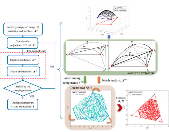
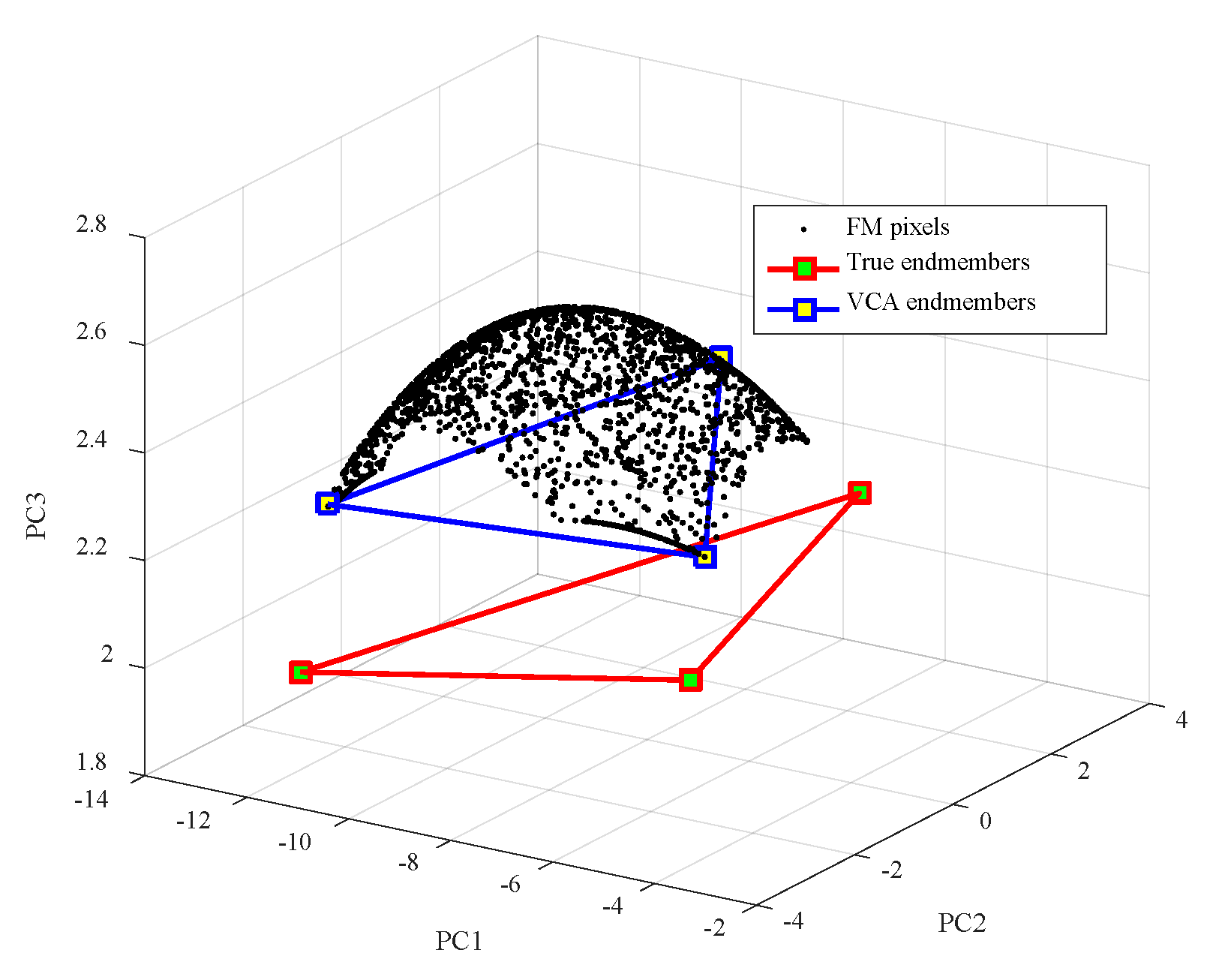
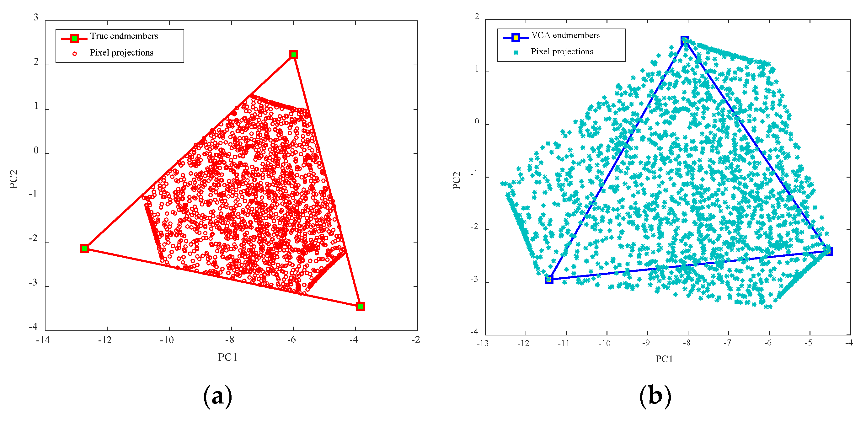
  • The negative effect of collinearity in BMM-based nonlinear unmixing methods can be addressed. To be specific, this goal is reached by adopting a distance measure to project pixels onto their approximate linear mixture components based on the geometric characteristics of the BMMs. This procedure reduces effectively the virtual endmembers’ impact on nonlinear unmixing, which is a remarkable advantage compared with other relevant unmixing methods.
  • The issue of local minima in standard NMF can be well alleviated, and highly mixed nonlinear hyperspectral data can be unmixed accurately. To be specific, the procedure of geometric projection facilitates the direct use of NMF in nonlinear unmixing, and the incorporation of a minimum endmember distance constraint into the NMF framework enables the accurate estimation of endmembers and abundances when pixels are highly mixed.
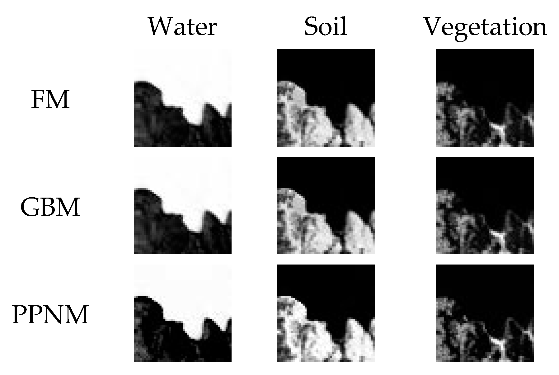
  • A general unsupervised nonlinear unmixing strategy is built which is simultaneously suitable for unmixing under the assumptions of three BMMs including the FM, GBM, and PPNM.
It should be noted that this paper is quite different from our previous published conference paper [67] which only gave a simple and immature description of the method. In this paper, a more detailed and comprehensive motivation is explained. In particular, an essential theory (Theorem 1 and Property 1 in Section 3) of constructing nonlinear hyperplanes and geometric projection to address the collinearity is provided with a proof. Several key issues of projection in theoretical and technical parts are also carefully discussed and further improved. Moreover, more reasonable experiments with simulated and real hyperspectral data are carried out here to validate the proposed algorithm’s superiority in unsupervised nonlinear unmixing compared with other state-of-the-art methods.
In terms of unsupervised spectral unmixing methods in the literature, their main drawbacks are in three aspects: (1) LMM-based unsupervised unmixing methods fail in explaining the nonlinear mixing effect; (2) Existing BMM-based unsupervised nonlinear unmixing methods always suffer from the negative effect of collinearity; (3) The issue of local minima is commonly serious for unsupervised nonlinear unmixing algorithms via NMF which may perform worse in unmixing highly mixed data.
The precise objective of this work is to propose a BMM-based unsupervised nonlinear unmixing algorithm via geometric projection and NMF, which could overcome the problem of the collinearity, and give better unmixing results when the pixels are nonlinearly and highly mixed.
The rest of this paper is organized as follows. The LMM, three BMMs, and NMF are introduced in Section 2. In Section 3, the issue of collinearity is analyzed, geometric projection for generating pixels’ approximate linear components is described, and the proposed algorithm combining geometric projection with constrained NMF for nonlinear unmixing is presented. In Section 4, in comparison with traditional and state-of-the-art algorithms, the proposed algorithm is evaluated through experiments. Finally, experimental results and future research directions are discussed in Section 5, and this paper is concluded in Section 6.

2. Related Works

2.1. Mixture Models

Generally, a hyperspectral image can be denoted as a matrix X n × m , each column of which corresponds to a pixel vector x j n × 1 ( j = 1 , 2 , , m ) with n spectral bands. m denotes the number of pixels. In this paper, three typical BMMs, including the FM [30], GBM [31], and PPNM [32], have been taken into account. It is noted that the LMM is these models’ common part, which is linearly combined by endmembers [1]. The nonlinearity is denoted as the sum of the products of every two endmembers, abundances, and corresponding nonlinear parameters. Therefore, these mixture models can be easily given a general expression for simplicity:
x j = i = 1 r a i s i , j + i = 1 t 1 k = t 2 r b i , k , j ( a i a k ) s i , j s k , j + ε j
s i , j 0 , i = 1 r s i , j = 1
Table 1 lists the specific definitions of general parameters t 1 , t 2 and b i , k , j in Equation (1) with respect to four mixture models. If b i , k , j = 0 , Equation (1) is the LMM. When t 1 = r 1 and t 2 = i + 1 , Equation (1) becomes the FM if b i , k , j = 1 , while it is the GBM if b i , k , j = γ i , k , j . Equation (1) denotes the PPNM when t 1 = r , t 2 = 1 and b i , k , j = ξ j .
In Equation (1), a i n × 1 is the i th endmember vector and s i , j is its abundance in the pixel x j . r is the number of endmembers. To be physically meaningful, abundances of these models should satisfy the nonnegative constraint (ANC) and sum-to-one constraint (ASC) in Equation (2). represents the Hadamard product operation and a i a k = ( a i , 1 a k , 1 , , a i , n a k , n ) T denotes the second-order interactions between endmember a i and a k , which is a so-called virtual endmember [50,51,52]. Both γ i , k , j [ 0 , 1 ] and ξ j are bilinear parameters used for scaling the nonlinearity, which make the GBM and PPNM more flexible than the FM. ε j n × 1 is the additive noise. It can be seen that when γ i , k , j = 0 and ξ j = 0 , i , k , j , both the GBM and PPNM transform into the LMM, and when γ i , k , j = 1 , i , k , j , the GBM is equivalent to the FM. In Figure 1, it can be observed how pixels based on four models distribute in a three-dimensional feature subspace, respectively.

2.2. NMF

NMF [13] aims to approximate a nonnegative matrix V n × m with the product of two unknown low rank, nonnegative matrices W n × r and H r × m in Equation (3). The square of the Euclidean distance between V and W H in Equation (4) is often used to quantify the approximation.
V W H
min W , H 1 2 V W H F 2 , s . t . W 0 , H 0
Clearly, NMF has the same structure as the LMM. In terms of the LMM-based spectral unmixing, V is the hyperspectral data, W can be regarded as the endmember matrix, and H represents the abundance matrix. Then, both the endmembers and abundances can be achieved simultaneously using the alternate update rules of NMF [13,68] and the nonnegative constraint is naturally satisfied.

3. Proposed Algorithm for Unsupervised Nonlinear Spectral Unmixing

3.1. Motivation for the Proposed Algorithm

Spectral unmixing is a process of multiple regression in some sense, where endmembers function as the explanatory variables and abundances are the regression coefficients [51,52,53]. The collinearity exists as a common problem for regression analysis when some explanatory variables can be largely explained by the others, causing the accretion of estimation error. In terms of the LMM-based spectral unmixing, it is often considered that true endmembers of different ground covers are usually affinely independent [2]. So sufficient accuracy can usually be provided, ignoring the effect of collinearity when executing the linear spectral unmixing.
However, this is not the case for the BMM-based nonlinear spectral unmixing, where the virtual endmembers are highly correlated with true endmembers. A virtual endmember [50,51,52] is the product of two true endmembers in each band. Although the high correlation between virtual and true endmembers (close to being linearly dependent) may make them have spectral similarity (see Figure 2), virtual endmembers have no physical meaning in terms of ground covers.
Moreover, since virtual endmembers are commonly used as the explanatory variables to estimate abundances with true endmembers, the negative impact of collinearity is inevitable, though no perfect collinearity exists [51]. Specifically, there will be a dramatic drop in the accuracy of estimated abundances, because a 1 , , a r , a 1 a 2 , , a t 1 a r in Equation (1) may produce a matrix approaching singularity, resulting in the results being unstable and sensitive to noise [50,51,52,53]. This situation can get worse when numerous nonlinear parameters should be estimated and true endmembers are unknown. The degree of collinearity induced by virtual endmembers will be discussed using a quantitative measure named variance inflation factors (VIFs) [51,52] in Section 4.1.
One intuitive idea for nonlinear spectral unmixing which always comes into being is that if the nonlinearly-mixed pixels can be transformed into the linearly mixed ones, or their nonlinearity can be removed, the conventional linear methods can be used for unmixing. If so, this not only provides the possibility of carrying out the unsupervised unmixing via the constrained NMF, but the collinearity will also not affect the unmixing. To this end, the geometric characteristics of BMMs are exploited to achieve that goal.
Geometrically, each pixel can be considered as a point in an n-dimensional space. Under the assumption of the LMM, endmembers { a 1 , a 2 , , a r } construct a ( r 1 ) -dimensional simplex Δ r 1 = { x = i = 1 r a i s i | i = 1 r s i = 1 , s i 0 } in the feature subspace to meet the constraints in Equation (2) and enclose all the pixel points. Abundances are equivalent to the pixels’ normalized barycentric coordinates with respect to the endmembers on Δ r 1 [59,61,62]. As shown in Figure 1a, the simplex Δ 2 spanned by three endmembers is a triangle [65,66,67,68].
On the other hand, in terms of the BMMs, the contribution of the nonlinear part will explicitly lead pixel points to move out of Δ r 1 and distribute in a higher dimension space forming different nonlinear manifold structures in Figure 1b–d. It is known that the linear mixture part x j L M M = i = 1 r a i s i , j of a BMM-pixel is equivalent to the definition of LMM, so the x j L M M of a pixel x j belongs to the Δ r 1 constructed by { a 1 , a 2 , , a r } . As a result, a BMM pixel point x j can be simply regarded as the result by pulling the point x j L M M out from Δ r 1 to an r -dimensional affine hull along the vector corresponding to x j ’s nonlinear part. Mathematically, BMM pixels belong to the linear subspace spanned by both true and virtual endmembers, whose dimension is r ( r + 1 ) / 2 for the FM and GBM and r ( r + 3 ) / 2 for the PPNM. However, in the r -dimensional feature subspace, BMM pixels actually lie on the same r -dimensional affine hull constructed by r true endmembers and an additional affinely independent vector.
According to the BMMs’ geometric characteristics, the following Property 1 and Theorem 1 were concluded in the authors’ previous work [58]. A brief introduction is provided here.
Property 1.
In the r -dimensional feature subspace, a BMM pixel x j can be affinely represented on an r -dimensional affine hull C r = aff { a 1 , a 2 , , a r , p j } = { x j = i = 1 r a i h i + p j h r + 1 | i = 1 r + 1 h i = 1 } constructed by r true endmembers and an extra vertex p j (called the nonlinear vertex). Moreover, x j ’s abundances s j and its normalized barycentric coordinates h j = ( h 1 , j , h 2 , j , h r + 1 , j ) T on the C r ( h r + 1 , j is x j ’s normalized barycentric coordinate with respect to p j ) satisfy s i , j = h i , j / k = 1 r h k , j , when this p j also lies on the line defined by x j and its corresponding linear mixture component x j L M M .
This property can be easily obtained according to the geometric theory of simplex [59,60,61,62]. As shown in Figure 3, if x j ’s affine-projection y j on the Δ r 1 is equal to x j L M M , y j ’s normalized barycentric coordinates ( h 1 , j / k = 1 r h k , j , h 2 , j / k = 1 r h k , j , , h r , j / k = 1 r h k , j , 0 ) T on the C r is equal to ( s 1 , j , s 2 , j , , s r , j , 0 ) T . However, it can be deduced that the vertex p j is pixel-dependent, and each pixel can have an infinite number of satisfactory nonlinear vertices as long as such a p j is not only affinely independent of { a 1 , a 2 , , a r } , but also lies on the line defined by the points x j L M M and x j (see Figure 3). On the other hand, x j L M M is unknown for most pixels, and determining each x j ’s own correct nonlinear vertex p j is impossible.
In order to circumvent this issue, a unique and common nonlinear vertex p was constructed in the authors’ previous work [58] to project all the pixels onto the Δ r 1 simultaneously. This single vertex p can concentrate most nonlinear components from the virtual endmembers, and BMM pixels’ projections deviate slightly from their true linear mixture components [58]. Theorem 1 has illustrated the construction of such a single nonlinear vertex p based on the idea of computer-aided geometric design [63].
Theorem 1.
Given r endmembers in the r -dimensional feature subspace, and assuming that a vertex p is the intersection of r ( r 1 ) -dimensional hyperplanes H 1 r 1 , , H r r 1 , each of which is formed by ( r 1 ) endmembers and the corresponding BMM pixels constituted by them (e.g., { a 1 , a 2 } and ω 3 define the plane H 3 2 in Figure 4), p will span an r -dimensional affine hull C r = aff { a 1 , a 2 , , a r , p } with r endmembers to affinely represent these pixels (see Property 1).
Proof. 
Let a pixel in Equation (1) x j ’s nonlinear part x j N M M = i = 1 t 1 k = t 2 r b i , k , j ( a i a k ) s i , j s k , j and x j = x j L M M + x j N M M , when the endmembers’ number r = 2 (see Figure 3), x j N M M = a 1 a 2 s 1 , j s 2 , j b 1 , 2 , j for the FM and GBM. In this case, the linear part x j L M M = a 1 s 1 , j + a 2 s 2 , j lies on the Δ 1 that is a line segment defined by a 1 and a 2 . It is clear that x j and two endmembers { a 1 , a 2 } are located on the same two-dimensional plane H 2 in the three-dimensional feature subspace. The vertex p can be the intersection of two tangential (or vertical) lines (i.e., H 1 1 and H 2 1 ) passing through the endmember a 1 and a 2 , respectively. Then, a two-dimensional affine hull aff { a 1 , a 2 , p } is always obtained to represent all the pixels. It is noted that by using such a vertex p , x j can be largely projected to x j L M M on the Δ 1 [58]. In terms of the PPNM, x j N M M = i = 1 2 k = 1 2 b i , k , j ( a i a k ) s i , j s k , j and the coplanarity is still reliable because a i a i is very likely to be highly dependent on a i .
When r = 3 (see Figure 4a), in the three-dimensional feature subspace, two-endmember sets { a 1 , a 2 } , { a 1 , a 3 } , and { a 2 , a 3 } form three two-dimensional hyperplanes H 3 2 , H 2 2 , and H 1 2 with corresponding pixels in the same way, respectively. If noise is ignored, BMM pixels constituted by all three endmembers { a 1 , a 2 , a 3 } (i.e., affected by all virtual endmembers) must be located in the local space enclosed by { H 1 2 ,   H 2 2 ,   H 3 2 } . In this case, the vertex p becomes the intersection of planes { H 1 2 ,   H 2 2 ,   H 3 2 } , and { a 1 , a 2 , a 3 , p } span a three-dimensional affine hyperplane C 3 , including all the pixels in the feature subspace.
When r 4 , the formation of a simplex that any Δ r 1 is enclosed by r ( r 2 ) -dimensional simplices, and Δ r 1 is a facet of Δ r [9,59] can be applied for understanding. p is the intersection of r ( r 1 ) -dimensional hyperplanes H 1 r 1 , , H r r 1 in the r -dimensional feature subspace. H q r 1 is defined by ( r 1 ) endmembers { a 1 , , a q 1 , a q + 1 , , a r } and any corresponding BMM pixels constructed by them in Equation (1). For instance, { a 1 , a 2 , a 3 , a 4 , p } span a four-dimensional affine hyperplane C 4 where the vertex p is the intersection of planes { H 1 3 , H 2 3 , H 3 3 , H 4 3 } and H 4 3 is actually the plane of the previous C 3 . Thus, all the pixels are affinely represented on an r -dimensional affine hull aff { a 1 , , a r , p } . H 1 r 1 , , H r r 1 will always intersect at a single point because they intersect each other and their normal vectors are linearly independent in the r -dimensional subspace [59]. In [58], the conclusion that the system of linear equations for calculating the nonlinear vertex p always has a unique non-trivial solution also demonstrates the uniqueness. □
In this paper, Theorem 1 is partly utilized to estimate the BMM-pixels’ normalized barycentric coordinates h with respect to { a 1 , a 2 , , a r } on the affine hull C r . One way to solve h is to calculate the nonlinear vertex p directly, and then using the traditional linear unmixing methods such as the constrained least squares [6] to get h . In fact, after the hyperplanes H 1 r 1 , , H r r 1 are determined, pixels’ projection coordinates can be obtained by volume- or distance-based geometric linear unmixing methods (see Figure 4b) [7].
A hyperplane H q r 1 actually represents the nonlinearity not relevant to the endmember a q , which is called a nonlinear hyperplane in the rest of the paper. As discussed earlier, the abundances of the BMM pixels on H q r 1 with respect to a q should be equal to zero. Specifically, following the simplex theory [7,59,60,61,62,63,64,65,66], the ratio of the distances (signed distance measure in [7] is used in this paper) from the pixel x j and a q to the H q r 1 is x j ’s normalized barycentric coordinate h q , j with respect to a q . In this sense, h q , j is also x j ’s projection coordinate s ^ q , j , which is approximately equal to the abundance s q , j . Then, h j can be used to obtain a pixel’s projection y j on the Δ r 1 spanned by { a 1 , a 2 , , a r } , which is its approximate linear component y j = i = 1 r a i h i , j i = 1 r a i s i , j . It allows the further use of the conventional linear unmixing methods to obtain more accurate results.
Accordingly, the virtual endmembers are absent from the abundance estimation, leading to the decrease of collinearity’s negative effect to a much lower level [58]. As a result, the unmixing accuracy will get great improvement. On the other hand, it is worthy of noting that by exploiting the distance measure, projections can be achieved without determining the nonlinear vertex p or reducing the dimension of data to r . This advantage makes the later proposed method able to update the endmembers in their original space, which will reduce not only the computational burdens, but also the estimation errors of endmembers in unsupervised unmixing.
The goal of this paper is to unmix the BMM pixels in an unsupervised way. In this sense, both endmembers and abundances are unknown and, as stated in the previous section, algorithms such as VCA may wrongly extract endmembers when pure pixels do not exist in the hyperspectral data.
For example, in Figure 5, the FM-based pixels close to the true endmembers are wrongly extracted as the endmembers. Moreover, as shown in Figure 6, when endmembers are not true, pixels’ projections will move out of the simplex spanned by endmembers. Nevertheless, since pixels’ projections are linearly mixed, they can be substituted into the constrained NMF framework to update the endmembers and abundances. Then, updated endmembers can be further used to calculate the new projections until the endmembers’ simplex Δ r 1 can contain all the pixels’ projections compactly. By doing this, more accurate endmembers can be found even if hyperspectral pixels are highly mixed, and better unmixing results will be obtained in an unsupervised way. Figure 7 depicts the main procedure of the proposed method.

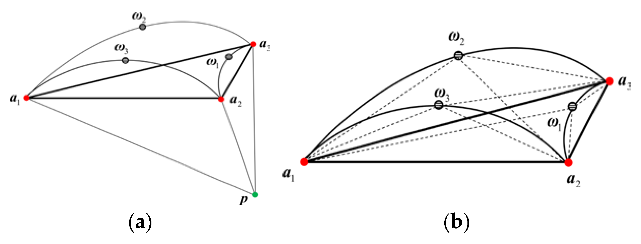
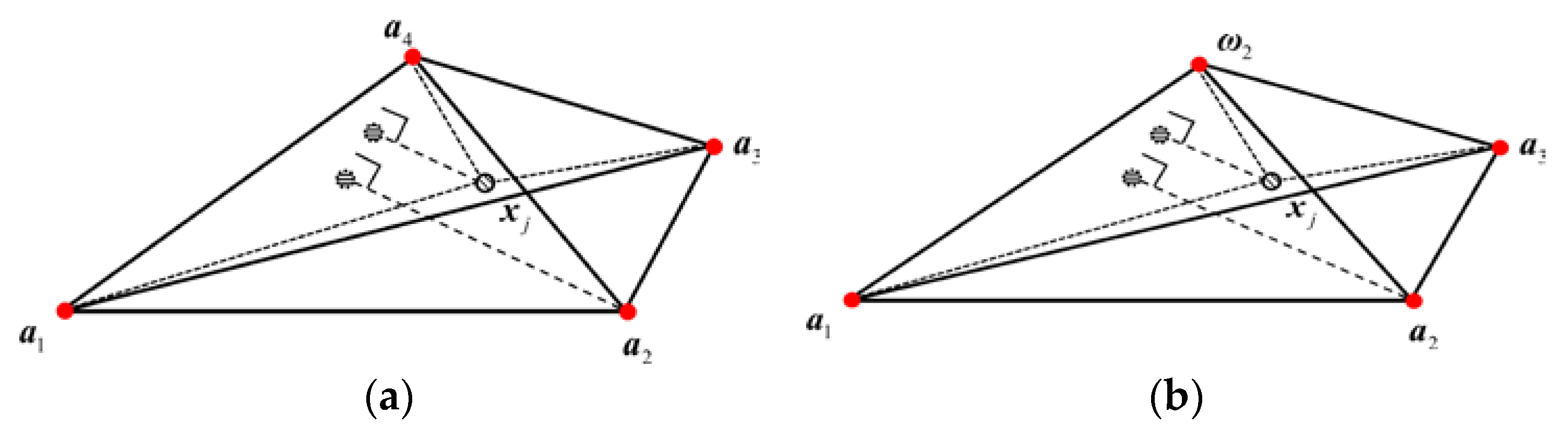
3.2. Nonlinear Hyperplanes and Geometric Projection

In this section, the method of determining the aforementioned nonlinear hyperplanes H 1 r 1 , , H r r 1 and the approach to calculate BMM pixels’ normalized barycentric coordinates with respect to endmembers { a 1 , a 2 , , a r } is introduced, as well as their projections on the bottom affine plane (see Figure 5 and Figure 6) defined by { a 1 , a 2 , , a r } .
Firstly, according to the previous analysis and Theorem 1, a nonlinear hyperplane H q r 1 in the r -dimensional feature subspace is defined by the ( r 1 ) -endmember subset { a 1 , , a q 1 , a q + 1 , , a r } and corresponding BMM pixels constituted by these ( r 1 ) endmembers. In other words, only a proper BMM pixel (named the control point) constituted by { a 1 , , a q 1 , a q + 1 , , a r } is needed to further determine the hyperplane H q r 1 .
To be specific, the idea of computer-aided geometric design [63] is used here to determine the nonlinear hyperplanes. As shown in Figure 4, r nonlinear midpoints ω q ( q = 1 , , r ) are chosen as the control points [63]. They consist of every ( r 1 ) endmembers with the same abundances, i.e., s 1 , ω q = = s q 1 , ω q = s q + 1 , ω q = = s r , ω q = 1 / ( r 1 ) . Based on Equation (1), ω q can be expressed as:
ω q = 1 r 1 i = 1 r a i + 1 ( r 1 ) 2 i = 1 t 1 k = t 2 r ( a i a k )
where i q and k q , q = 1 , , r . When t 1 = r 1 and t 2 = i + 1 , Equation (5) is the case of the FM and GBM, and when t 1 = r , t 2 = 1 , it corresponds to the PPNM. Then, we use the constructed nonlinear midpoint ω q to determine the hyperplane H q r 1 with ( r 1 ) endmembers { a 1 , , a q 1 , a q + 1 , , a r } . For instance, H 2 2 in both Figure 4 and Figure 8b refers to the plane defined by { a 1 , ω 2 , a 3 } . At the same time, the selection of nonlinear midpoints { ω 1 , ω 2 , , ω r } as the control points also guarantees the formation of r non-degenerate r -dimensional simplices [59]. As depicted in Figure 4b, { a 1 , a 2 , a 3 , ω 1 } , { a 1 , a 2 , a 3 , ω 2 } , and { a 1 , a 2 , a 3 , ω 3 } form three three-dimensional simplices Δ ˜ 1 3 , Δ ˜ 2 3 , and Δ ˜ 3 3 , respectively. A facet of Δ ˜ 2 3 is on the H 2 2 . In the feature subspace, the q th simplex Δ ˜ q r is constructed by the point set M q = ( m 1 , q , , m l , q , , m r , q , m ( r + 1 ) , q ) = ( a 1 , , a r , ω q ) , M q n × ( r + 1 ) , l = 1 , 2 , , r + 1 .
Secondly, according to the geometric explanation of the LMM, for example, if a pixel x j is linearly mixed by four endmembers (see Figure 8a), a 2 ’s fractional abundance in x j is equal to the ratio (i.e., projection coordinates [7]) of distances from x j and a 2 to the plane of the bottom triangle defined by { a 1 , a 3 , a 4 } . Similarly, on the constructed r -dimensional simplex Δ ˜ q r , the distances from each BMM pixel point to the nonlinear hyperplane H q r 1 can be used to calculate pixels’ projection coordinates with respect to endmember a q . When the BMM pixels’ projection coordinates are obtained, they will be approximately projected to their linear parts on the Δ r 1 constructed by { a 1 , a 2 , , a r } .
Assuming that an endmember matrix A = ( a 1 , , a r ) n × r is given, the signed distance measure proposed in [7] is adopted to calculate pixels’ projection coordinates. In line with the least squares criterion, this distance measure enables the abundance estimation to be implemented in a subspace at a high speed, without dimension reduction. In our method, the whole process of estimating BMM pixels’ projection coordinates are split into r sub-steps. Specifically, the distance measure is applied for r constructed simplices Δ ˜ 1 r , Δ ˜ 2 r , , Δ ˜ r r , respectively. For the Δ ˜ q r , only pixels’ projection coordinates associated with endmember a q are calculated, and the distance measure has the following form:
{ k l , q T m l , q + b l , q = 1 k l , q T m τ , q ( τ l ) + b l , q = 0 , l = 1 , , r + 1
where k l , q n × 1 represents the weight vector of the l th facet of Δ ˜ q r . The scalar b l , q is a threshold value. m l , q is the l th column of M q = ( a 1 , , a r , ω q ) . One can see that Equation (6) is definitely an extended version of the single simplex under the assumption of LMM in [7]. It should be noted that k q , q corresponds to the weight vector of the hyperplane H q r 1 opposite to the endmember a q . For instance, Figure 8b shows a constructed simplex Δ ˜ 2 3 spanned by M 2 = ( a 1 , a 2 , a 3 , ω 2 ) , where k 2 , 2 is the weight vector of the hyperplane H 2 2 containing the nonlinear midpoint ω 2 . Based on Equation (6), the distance from a 2 to H 2 2 is 1, while the distances from { a 1 , ω 2 , a 3 } to H 2 2 are equal to zero because they actually lie on H 2 2 . Therefore, when k 2 , 2 and b 2 , 2 in Equation (6) are calculated, a BMM pixel x j ’s projection coordinate s ^ 2 , j with respect to the endmember a 2 can be further produced by s ^ 2 , j = k 2 , 2 T x j + b 2 , 2 .
For the Δ ˜ q r , let V q = ( m 1 , q m ( r + 1 ) , q , m 2 , q m 1 , q , , m ( r + 1 ) , q m r , q ) n × r . All the column vectors of V q can be regarded as the base vectors spanning the r -dimensional subspace in which k l , q ( l = 1 , , r + 1 ) must lie. k l , q can be linearly represented by r column vectors of V q , which is further written as:
k l , q = V q β l , q , β l , q = ( β l , q 1 , , β l , q r ) T r × 1 .
In Equation (7), β l , q denotes the coefficients of k l , q with respect to V q ’s column vectors, and at least one nonzero coefficient exists [7]. By substituting (7) into (6), and letting K q = ( k 1 , q , , k ( r + 1 ) , q ) n × ( r + 1 ) , b q = ( b 1 , q , , b ( r + 1 ) , q ) T ( r + 1 ) × 1 , and B q = ( β 1 , q , , β ( r + 1 ) , q ) r × ( r + 1 ) , Equations (8) and (9) are obtained:
( M q T V q ) B q + b q 1 r + 1 T = I ( r + 1 ) × ( r + 1 )
( B q b q T ) = ( M q T V q , 1 r + 1 ) 1 , K q = V q B q .
where 1 r + 1 is a column vector of all 1s and I ( r + 1 ) × ( r + 1 ) is a unit matrix.
Finally, after k q , q and b q , q are obtained, pixels’ projection coordinates of the q th endmember a q can be obtained, which are equal to k q , q T X + b q , q 1 m T . Furthermore, different from [7], let z q = k q , q and c q = b q , q , and the whole projection coordinate vector s ^ j of a BMM pixel x j in our modified method is given as:
s ^ j = Z T x j + c
where Z = ( z 1 , , z r ) n × r and c = ( c 1 , , c r ) T r × 1 . The projection of x j is derived:
y j = A s ^ j
It is noted that if the used endmembers are true, they will construct a compact simplex Δ r 1 to enclose all the pixels’ projections y j (see Figure 6a) [1,2,3,4,5]. However, if endmembers are unknown or wrongly extracted (see Figure 6b), we should further estimate the endmembers. Fortunately, with the use of the obtained linearly-mixed projections of pixels, the minimum-volume-constrained NMF [8,9,10,11,12] can be further adopted to update the endmembers and abundances simultaneously for highly-mixed data. The newly-updated endmembers can be applied to project pixels to their new linear mixture components (i.e., Equation (11)), alternately.
According to the discussion in Section 3.1, there is a minor bias between a BMM pixel x j ’s projection y j in Equation (11) and its true linear mixture component x j L M M . This bias is mainly induced by two aspects: constructing several hyperplanes to produce a single nonlinear vertex p to replace all the virtual endmembers, and the noise interference. This bias has been carefully analyzed in [58], which further utilized two different strategies to do the de-biasing. The process of removing bias is iterative and has a larger calculation burden, and its performance relies on true endmembers already being known.
Therefore, the de-biasing is not taken into account in the proposed algorithm of this paper, based on two reasons. Firstly, the endmembers are assumed to be unknown here, and should be estimated in the later unsupervised unmixing. In this sense, the de-biasing should be executed at every iteration once endmembers are updated, resulting in high computational complexity. Secondly, using the inaccurate endmembers to do the de-biasing will not only fail in removing the bias, but also transfer the error into the estimation of endmembers and abundances. On the other hand, the accurate update of endmembers and abundances can be entirely implemented by using the obtained pixels’ projections due to their close proximity to the corresponding linear mixture components. In Section 4.1, with the use of true endmembers, the geometric projection coordinates (10) are quantitatively evaluated to illustrate the reasonability of omitting de-biasing in the proposed algorithm.

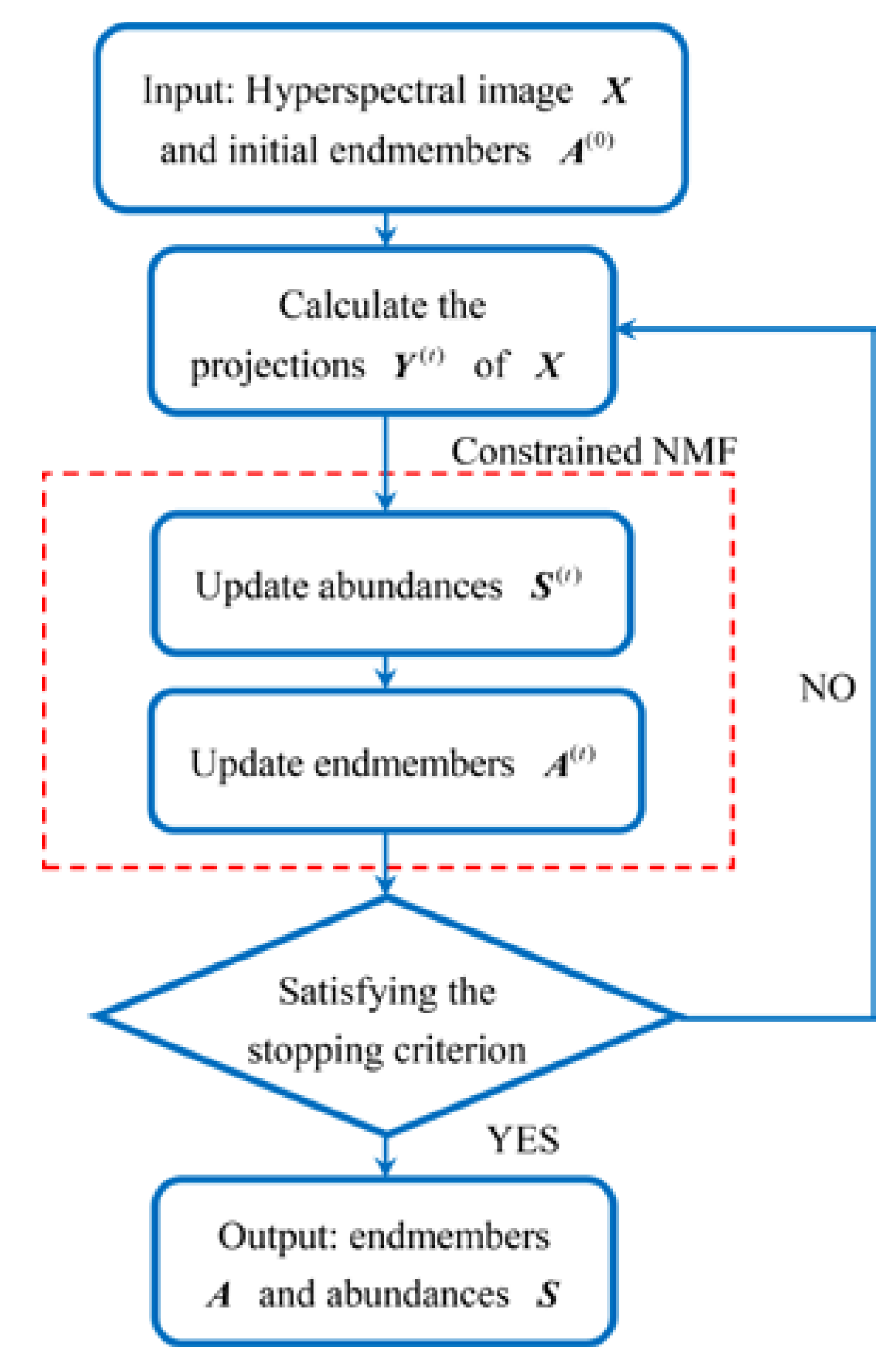
3.3. BMM-Based Constrained NMF

When addressing the issue of unsupervised unmixing, the noncovexity of standard NMF’s bi-affine objective function makes the solution nonunique, and an unsatisfied local minimum is always produced for unmixing [11,13]. In order to obtain more accurate results, additional physical constraints on endmembers or abundances should be incorporated into the objective function besides the ANC and ASC [11,12,13,14,15,16,17,18,19,20,21,22,23,24,25]. Consistent with the idea of using minimum-volume-constrained NMF for unmixing highly mixed data [11,12], Δ r 1 spanned by endmembers { a 1 , a 2 , , a r } should contain all the pixels’ projections compactly in the proposed algorithm. This implies that the reconstruction error in Equation (4) should be as small as possible, and the volume of Δ r 1 should decrease at the same time. Therefore, the endmember distance (EMD) in [12] is added into the standard NMF objective function (i.e., Equation (4)) as an auxiliary constraint, which is convex and represents the sum of distances from each endmember to their common centroid. Different from the optimization problem of constrained NMF for traditional linear unmixing, each pixel’s projection y j instead of pixel x j itself is adopted in the following situation:
min A ,   S f ( A , S ) = 1 2 Y A S F 2 + λ · E M D ( A ) , s . t . A 0 ,   S 0 ,   1 r T S = 1 n T
E M D ( A ) = i = 1 r a i a ¯ 2 2 , a ¯ = 1 r i = 1 r a i .
where S = ( s 1 , s 2 , , s m ) r × m is the abundance matrix and Y = ( y 1 , , y m ) n × m represents the matrix of pixels’ projections. The purpose of the endmember distance constraint EMD defined in (13) is to keep the simplex Δ r 1 of endmembers as compact as possible so as to limit the solution space. If the reconstruction error Y A S F 2 becomes smaller, Δ r 1 ’s volume will increase to include all the projections, while, if EMD decreases, Δ r 1 ’s volume will shrink. λ is a regularization parameter to balance the tradeoff between two terms in (12) to provide accurate endmembers.
Some existing algorithms such as the multiple update rule [13] and projected gradient (PG) method [48,57,68] can solve the optimization problem in (12). In this paper, the PG method is adopted to update endmembers A and abundances S alternately in the framework of constrained NMF. The gradients of f in (12) with respect to S and A are provided in Equations (14) and (15), respectively:
S f ( A t , S t ) = ( A t ) T ( A t S t Y t )
A f ( A t , S t ) = ( A t S t Y t ) ( S t ) T + λ · ( A t a ¯ 1 r T )
Specifically, the current values of S t + 1 or A t + 1 are updated using their corresponding values at the last iteration t . Following the PG update rules, S t + 1 and A t + 1 are updated in Equations (16) and (17) to satisfy the ANC.
S t + 1 = P [ S t α t · S f ( A t , S t ) ]
A t + 1 = P [ A t β t · A f ( A t , S t ) ]
X ˜ = [ X δ 1 T ] ,   A ˜ = [ A δ 1 T ]
In Equations (16) and (17), P [ · ] represents the operator for projecting S and A to be nonnegative. α t and β t are the updating steps which can be determined using the Armijo rule [48,57,68]. In simple terms, α t and β t decrease to give a better convergence when the relative error condition between two contiguous iterations in [68] is satisfied, or they will increase to accelerate the search. A t + 1 is further substituted into the geometric projection scheme (6)–(11) to generate the new projections Y t + 1 . The convergence analysis on the PG has been well analyzed in [68]. An experimental analysis is also provided for discussion of the convergence and complexity of the proposed algorithm in Section 4.1. Moreover, in order to satisfy the ASC, abundances should be normalized and two formulas in (18) [11,12,13,14,15,16,17,18,19,20,21,22,23,24,25] are substituted for operations (14)–(17) instead, where δ is used for balancing the effect of the ASC. Endmembers and abundances with sufficient accuracy will be obtained when the maximum number of iterations is reached, or the error between two iterations is less than a given threshold τ .
The nonlinear coefficients of the GBM and PPNM are not estimated in the proposed algorithm. In the case of the PPNM, if two pixels x j and x j + 1 have the same abundances s but different nonlinear scalar coefficients ξ j and ξ j + 1 (see Table 1), they still have the same projection y after being projected. In the case of the GBM, although the nonlinear coefficients γ i , k , j affect every virtual endmember, their influence on the projection is still minor because most nonlinear components have been explained by the nonlinear vertex p . On the other hand, endmembers and abundances are actually the core goals of unmixing, which are directly estimated in this work. When accurate endmembers and abundances are obtained, the nonlinear coefficients will be easily calculated by linear programming [65]. According to the flowchart in Figure 7, the proposed BMM-based constrained NMF algorithm (BCNMF) for the unsupervised nonlinear spectral unmixing is summarized in Algorithm 1.
Algorithm 1: BMM-based constrained NMF (BCNMF)
Input: Hyperspectral data X n × m and initial endmember matrix A 0 obtained by VCA.
Output: Abundance matrix S r × m and endmember matrix A n × r .
Step 1. Set t = 0 , initialize S 0 and Y 0 with Equations (10) and (11).
while stopping conditions are not met, do
Step 2. Update endmembers and abundances in the constrained NMF framework
  (2a) Update S t + 1 with Equation (16) [48,57,68].
  (2b) Update A t + 1 with Equation (17) [48,57,68].
Step 3. Calculate pixels’ projections
  (3a) Calculate r nonlinear midpoints ω q with Equation (5) [58].
  (3b) Update pixels’ projections Y t + 1 using Equation (11).
Step 4. t = t + 1 .
End

4. Experimental Results

In this section, the unmixing performance of the proposed algorithm BCNMF is evaluated by carrying out five experiments with the synthetic data, one experiment with a virtual citrus orchard data, and two experiments with real hyperspectral images, respectively. Moreover, to demonstrate the robustness of BCNMF, it is compared with a group of traditional and state-of-the-art linear or nonlinear spectral unmixing algorithms. Accordingly, four supervised algorithms, including the famous linear algorithm FCLS [6], GBM-based semiNMF [38], PPNM-based GDA [32], and MLM [37] are compared for the abundance estimation by using true endmembers or the endmembers extracted by VCA [4]. Besides, four state-of-the-art unsupervised nonlinear spectral unmixing algorithms, including the Fan-NMF [30], distance-based nonlinear simplex projection unmixing (DNSPU) [46], RNMF [54], and bi-objective kernel NMF (Bio-KNMF) [57] have also been considered. Most of these algorithms have been briefly described in the introduction. DNSPU adopts the geodesic distance to exploit the data manifold and estimate both endmembers and abundances. Bio-KNMF combines the objective functions of kernel NMF and NMF to formulate a bi-objective problem to be solved for unmixing. In the following experiments when the true endmembers are unknown, the endmembers extracted by VCA and abundances estimated by FCLS are used as the initialization for the Fan-NMF, RNMF, Bio-KNMF, and the proposed algorithm.
According to the recommendatory parameter settings reported in the compared algorithms’ corresponding references, we make their configurations as follows to produce the best results. The maximum numbers of iteration in Fan-NMF, RNMF, Bio-KNMF, and BCNMF are set to 300 and τ = 1 e 5 . δ that controls the ASC in GBM-semiNMF, BCNMF, and Fan-NMF is set to 10. λ that balances the additional constraints in BCNMF and RNMF is equal to 0.1 (detailed discussions are given in Section 4.1.5). For the DNSPU, the geodesic distance is used and K = 20 for the nearest-neighbor graph [46]. A Gaussian kernel with parameter σ = 3 is applied in Bio-KNMF, and the weight α is carefully selected from { 0 , 0.1 , , 0.9 , 1 } through cross-validation to obtain the best performance. The experiments were performed on a computer with a 4-GHz Intel Core i7 CPU and 32 GB of memory.
Since BCNMF is an unsupervised algorithm, both the accuracies of estimated endmembers and abundances should be analyzed. In order to provide the quantitative evaluation for different algorithms’ experimental results, two classical performance metrics are defined, i.e., endmembers’ mean spectral angle distance (MSAD) [11] in Equation (19) and root mean square error (RMSE) [6] of abundance in Equation (20). Over the years, they have been widely used for evaluating unmixing results in numerous published works [6,7,8,9,10,11,12,15,16,17,18,19,20,21,22,23,24,25]. MSAD measures the similarity between true and estimated endmembers, while RMSE denotes the approximation error between true and estimated abundances.
MSAD = 1 r i = 1 r cos 1 ( a i T a ˜ i a i a ˜ i )
RMSE = 1 m r i = 1 m s i s ˜ i 2 2
In Equations (19) and (20), a i and a ˜ i represent a true endmember and an estimated endmember, respectively. s i and s ˜ i are the true abundance and estimated abundance, respectively. Since the FCLS, GBM-semiNMF, PPNMGDA, and MLM are all supervised unmixing algorithms, only six algorithms’ MSADs of extracted endmembers are compared.
On the other hand, it is noted that the issue of unavailable true endmembers and abundances in real hyperspectral images always hinders convincible quantitative evaluation in practice. Many works had to use a metric-like reconstruction error (RE) or signal-to-reconstruction error (SRE) [69] as a reference criterion for evaluation. However, a small value of RE does not really mean that accurate endmembers and abundances are obtained due to the possible occurrence of over-fitting [34,38]. Therefore, we first use a recent physical-based simulated data of a virtual citrus orchard [33,34,70] for unmixing in Section 4.2. It can be considered as a quasi-real hyperspectral data for studying nonlinearity, and true endmembers and abundances are known. Then, in the case of two real hyperspectral images, the reconstructed linear mixture components (i.e., A ˜ S ˜ ) instead of the reconstructed images are used to calculate the SRE L M M (dB) in Equation (21) to give a fair comparison. A large SRE L M M indicates that an algorithm may not reflect the sufficient nonlinear components.
SRE L M M = 10 log 10 ( E ( X 2 2 ) / E ( X A ˜ S ˜ 2 2 ) )

4.1. Experiments with Synthetic Data

Three types of synthetic data based on the FM, GBM, and PPNM are generated. Nine material spectra are selected as the endmembers from the US Geological Survey (USGS) digital spectral library. Trees, grass, and several minerals are included (see Figure 9) which are common ground covers associated with the nonlinear mixing effect [26,27]. According to the Dirichlet distribution [4], 2000 pixels’ abundances are randomly generated for each data type. Generally, the maximum abundance is set to 0.8 so that no pure pixels exist, and data is highly mixed. Moreover, data with different degrees of mixing is also provided in the third experiment to evaluate the sensitivity of algorithms. In terms of the GBM, the nonlinear parameter γ i , k , j is uniformly drawn in the set [0, 1], while, the parameter ξ j of the PPNM is uniformly drawn from (−0.3, 0.3) as reported in the reference [32]. Finally, the endmembers, abundances, and nonlinear parameters are substituted into three BMMs to produce the corresponding pixels, and additive white Gaussian noise is further added to the data.
As illustrated in the previous sections, the collinearity acts as an essential obstacle in nonlinear spectral unmixing, because the virtual endmembers are highly correlated to true endmembers. Therefore, before conducting the experiments, the true endmembers’ minimum VIFs [51,52] are first adopted to compare the collinearity quantitatively when true and virtual endmembers are regarded as the explanatory variables. If a true endmember’s VIF is smaller, it is hard to be explained by other variables, and the effect of collinearity on it is negligible [51,52,53]. In Table 2, as the number of endmembers increases, VIFs always increase; but when only true endmembers are considered as the explanatory variables, VIFs are very small. On the contrary, when the virtual endmembers are used, VIFs increase dramatically to very high values, and it is much easier for true endmembers to be explained by the other variables because of the serious collinearity, resulting in the larger errors for unmixing. Even if there are only three endmembers, the collinearity is prominent when considering the virtual endmembers. Accordingly, in the proposed algorithm, since the geometric projection enables the virtual endmembers to be ignored, a great improvement in accuracy can be observed in the results of subsequent experiments.
Using the synthetic data, five experiments have been designed for evaluating the compared algorithms. In the first experiment, the effect of collinearity on unmixing is first analyzed by using different numbers of known true endmembers. In this sense, the procedures of updating endmembers in five unsupervised nonlinear unmixing algorithms FanNMF, DNSPU, RNMF, Bio-KNMF, and the proposed BCNMF are omitted. Only the results of estimated abundances are compared. Then, algorithms’ robustness to the number of endmembers is analyzed when endmembers are unknown. In the second experiment, the robustness of the algorithms to noise are compared by changing the Signal Noise Ratio ( SNR = 10 log 10 ( E [ x T x ] / E [ ε T ε ] ) ) [2]. Next, the third experiment is carried out to evaluate the influence of the degree of mixing on the algorithms’ unmixing performances. These experiments have been executed independently twenty times, and the results’ averages and standard deviations are listed in the subsequent tables. The complexity and convergence of the proposed algorithm are analyzed, and the computational time is also compared in the fourth experiment. Finally, the impact of regularization parameter λ on BCNMF is discussed in the last experiment.

4.1.1. Robustness to the Collinearity and the Number of Endmembers

In order to illustrate the proposed BCNMF’s advantage in addressing the collinearity, true endmembers are first adopted for each algorithm to compare the accuracy of the abundance estimation. The SNR is 40 dB in this experiment. The endmembers are not updated in five unsupervised algorithms. Particularly, geometric projection coordinates (i.e., Equation (10)) obtained by BCNMF are directly used as the estimated abundances without any iterations. Table 3 displays the corresponding results when the numbers of endmembers are changed. It can be observed that BCNMF always performs much better than the other three state-of-the-art unsupervised algorithms. Compared with the supervised algorithms such as PPNMGDA which resort to multiple iterations, BCNMF is just slightly worse when the number of endmembers is three or five. It seems that the projection bias turns to be remarkable in this case, because the de-biasing process is omitted in BCNMF (more accurate results obtained by using de-biasing are provided in [58]).
However, if there are more endmembers (seven and nine) when the collinearity is more serious (see Table 2), BCNMF has the best results compared with other algorithms. It can be concluded that when true endmembers are known (i.e., doing the supervised unmixing), the procedure of geometric projection in the proposed algorithms is still able to produce satisfactory estimated abundances without de-biasing. Moreover, the effect of collinearity is reduced through projecting BMM pixels into their approximate linear mixture components.
Next, data with the maximum abundance 0.8 are generated to evaluate the algorithms by changing the number of endmembers, and SNR is 40 dB. Table 4 shows the endmember extraction results. BCNMF performs the best, and it is clear that accurate endmembers can always be obtained because of the combination of geometric projection and constrained NMF. Geometric projection enables BCNMF to get over the collinearity. Using the linearly-mixed projections, minimum-distance-constrained NMF helps to find the endmembers and alleviate the local minima for highly-mixed data. VCA and DNSPU could not provide endmembers as accurate as other algorithms. This is because these two algorithms are based on the assumption that pure pixels exist in the data, which may be not suitable for the highly-mixed data. Moreover, in Table 5, the accuracies of estimated abundances are compared. Although algorithms like GBM-semiNMF, PPNMGDA and RNMF have shown competitive performances especially for their corresponding model-based data, BCNMF always provides the most accurate abundances. Comparing with the results in Table 3, it is observed that when endmembers are inaccurate, a large drop appears in the accuracies of estimated abundances produced by all other supervised or unsupervised algorithms. Nevertheless, this situation does not significantly impact the BCNMF’s results. Experimental results imply that the number of endmembers does not affect the BCNMF much. This can be explained because the issue of collinearity seems to be addressed by the process of geometric projection, and local minima have been alleviated by adding useful constraints into the NMF framework.

4.1.2. Noise Robustness Analysis

In this experiment, three different BMM-based synthetic data are generated by five endmembers, and the SNR is set as 60 dB, 50 dB, 40 dB, 30 dB and 20 dB, respectively, to study the noise’s impact on the proposed algorithm. In Table 6 and Table 7, MSADs and RMSEs of the compared algorithms are given. The proposed algorithm BCNMF has shown the best unmixing performance no matter what the data is. As the SNR decreases, both the accuracies of estimated endmembers and abundances provided by most algorithms tend to be worse. From the results, one can see that RNMF can obtain accurate endmembers for three types of data because it is a model robust algorithm. DNSPU seems to be affected by noise at a high level, especially when SNR is equal to 20 dB. For this case it also needs the presence of pure pixels, and the calculation of geodesic distance is sensitive to noise. Bio-KNMF has a good accuracy of abundances, but the estimated endmembers are the worst, indicating that endmembers may be mapped into the high-dimensional feature space in an inappropriate way. In terms of specific model-based algorithms such as the GBM-semiNMF and PPNMGDA, more accurate results appear in the unmixing for the corresponding model-based data. Since the MLM is a general model including all degrees of multiple scatterings, it shows good performances in unmixing different BMM-based data as well. Compared with RNMF and BCNMF, Fan-NMF does not add extra constraints into the NMF, which often makes it perform worse and fall into local minima easily. In this experiment, it can be seen that BCNMF is superior for all BMM-based data, and has good robustness to noise.

4.1.3. Analysis of Sensitivity to the Degree of Mixing

In this experiment, the performance of the compared algorithms for the BMM-based data with different degrees of mixing (max abundance) is discussed, especially when data are highly mixed and when pure pixels exist. To produce the synthetic data, max abundance ranges from 0.7 to 1, the number of endmembers is five and SNR is 40 dB. From Table 8, it can be seen that as the max abundance decreases, an obvious drop appears in the accuracy of endmembers extracted by VCA. Moreover, Fan-NMF, RNMF, and Bio-KNMF also show a similar tendency, because they are initialized by VCA but fail to get much better results. On the other hand, although endmembers extracted by VCA are also used for the initiation of BCNMF, it has not been affected because the pixels’ linearly-mixed projections motivate the update of endmembers to work in a reasonable way under the constrained NMF framework. The minimum distance constraint enables NMF to find accurate endmembers for data in different mixing degrees. Similar situations happen in the abundance estimation, and related results are shown in Table 9. When the degree of mixing is high, VCA could not find the correct endmembers, and RMSEs of estimated abundances decrease as well. In this experiment, BCNMF still performs the best, owing to the combination of geometric projection and constrained NMF, which has considerably decreased the negative effect of the collinearity and local minima on the unsupervised nonlinear spectral unmixing.

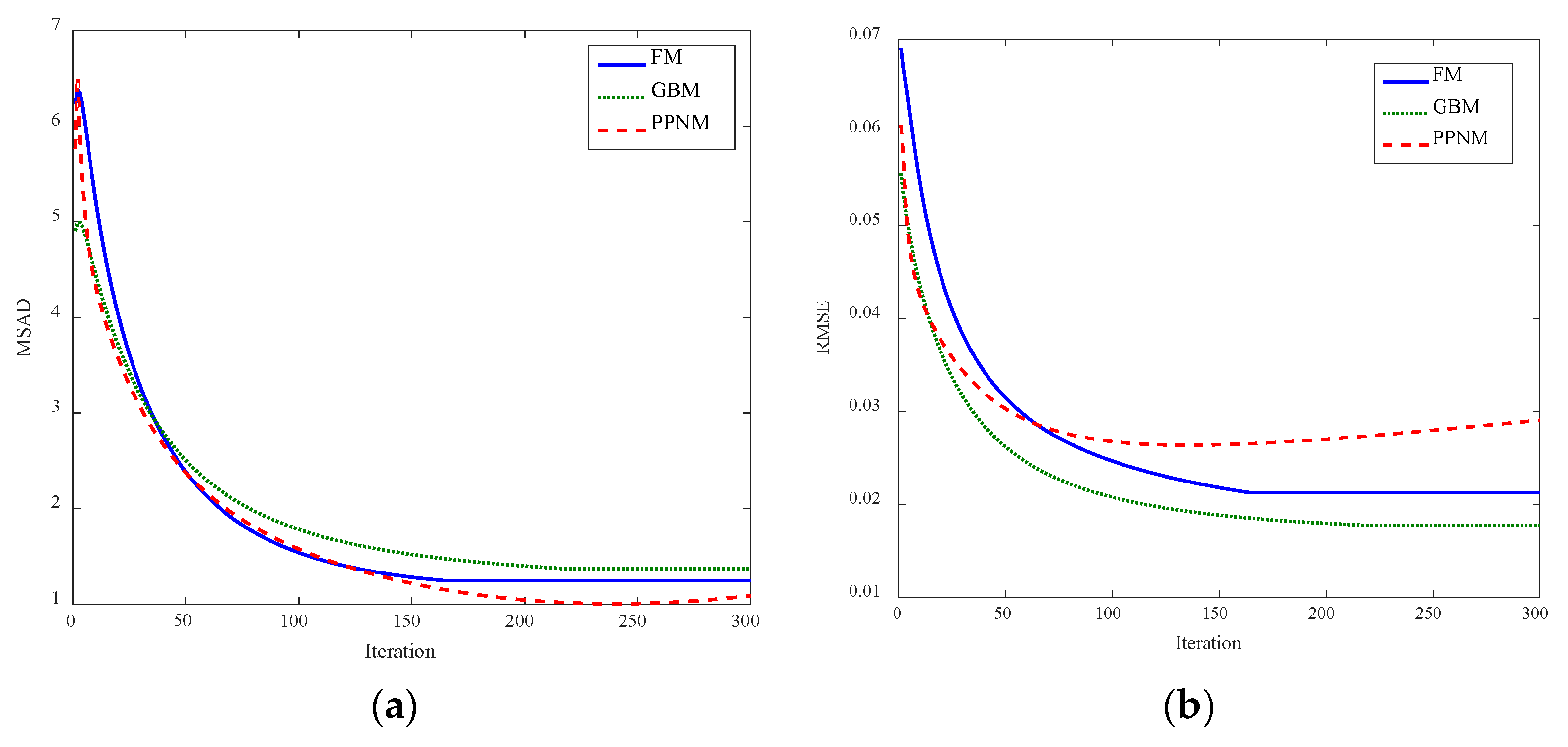
4.1.4. Complexity and Convergence Analysis

The complexity and convergence of the proposed algorithms are first analyzed in this experiment. During t iterations of BCNMF, three update steps for calculating the pixels’ projections Y (5)–(11), endmembers A (17), and abundances S (16) cost the most time. To be specific, in the process of geometric projection, the computational costs of Equations (5), (9)–(11) are O ( t r 2 n ) , O ( t ( r ( r + 1 ) n 2 + ( r + 1 ) 3 + n r 2 ( r + 1 ) ) ) , O ( t r m n 2 ) , and O ( t r 2 m n ) , respectively. So, the computational complexity of projection is O ( t ( r ( r + 1 ) n 2 + ( r + 1 ) 3 + n r 2 ( r + 2 ) + r m n 2 + r 2 m n ) ) . On the other hand, under the minimum-distance-constrained NMF framework, the total computational cost of updating A and S based on the PG is O ( 2 t ( κ r 2 ( m + n ) + r m n + r n ) ) where O ( 2 t r n ) is the cost of calculating the distance constraint (13). κ represents the average number of the checked condition [68] for updating the step sizes α t and β t per iteration.
In order to further compare the computational time of the algorithms, the number of pixels changes from 1000 to 4000 when the number of endmembers is five and SNR is 40 dB in the following experiment. Table 10 displays the algorithms’ time costs for unmixing three different BMMs data. It can be observed that as the number of pixels increases, more time is always needed for each algorithm. In all cases, FCLS has the best speed without considering the nonlinearity. But nonlinear unmixing methods such as PPNMGDA and Bio-KNMF need more time for calculation. Notably, the time cost of BCNMF is considerably low compared with other NMF-based methods and the algorithms which have good unmixing accuracies (e.g., PPNMGDA and MLM) in the previous experiments. It implies that BCNMF may be a fast and efficient nonlinear unmixing algorithm.
An experiment is further carried out to illustrate the convergence of BCNMF. Five endmembers are used to generate three BMM-based data and the SNR is 40 dB. In Figure 10, the changing curves of MSADs and RMSEs obtained by BCNMF for the FM, GBM, and PPNM based data are depicted. Both the MSAD and RMSE have converged to the stable small values quickly. In Figure 10b, the initial RMSEs are small because the abundances are initialized by the geometric projection, which has the capability to project pixels onto their approximate linear mixture components (see details in Section 3). Moreover, since the step of geometric projection is in line with the least squares [7] and the convergence of PG to a stationary point for endmember-distance-constrained NMF is also satisfied, referring to [12,68], the proposed algorithm BCNMF can always converge to get satisfactory unmixing results after a sufficient number of iterations.

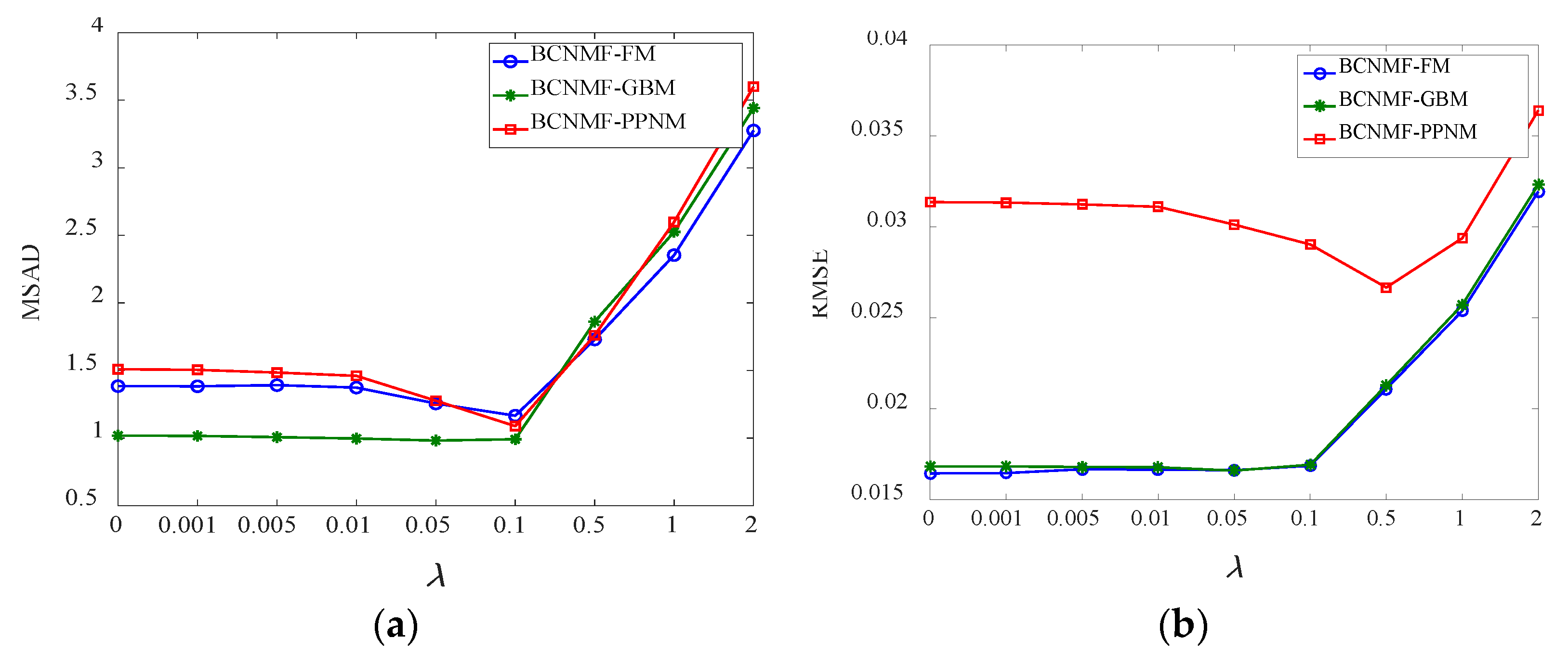
4.1.5. Parameter Sensitivity Analysis

This experiment is used to analyze the sensitivity of BCNMF’s performance to variations of regularization parameter λ in Equation (12). A proper λ will help to find more accurate endmembers even if pixels are highly mixed. The number of endmembers is five and SNR is 40 dB. The value of λ is well selected from { 0 , 0.001 , 0.005 , 0.01 , 0.05 , 0.1 , 0.5 , 1 , 2 } . Figure 11a,b shows the change of the accuracy of estimated endmembers and abundances, respectively. It can be observed that the overall best unmixing results are obtained when λ is around 0.1 for three BMMs. A larger λ may quickly decrease the accuracy. Although the RMSEs of abundances are still small when λ = 0 , i.e., EMD in Equation (12) is not considered, MSADs of estimated endmembers are worse than the case of λ = 0.1 . It is indicated that the use of minimum distance constraint in the NMF framework indeed helps to alleviate the local minima and especially improve the endmember extraction for highly mixed data.

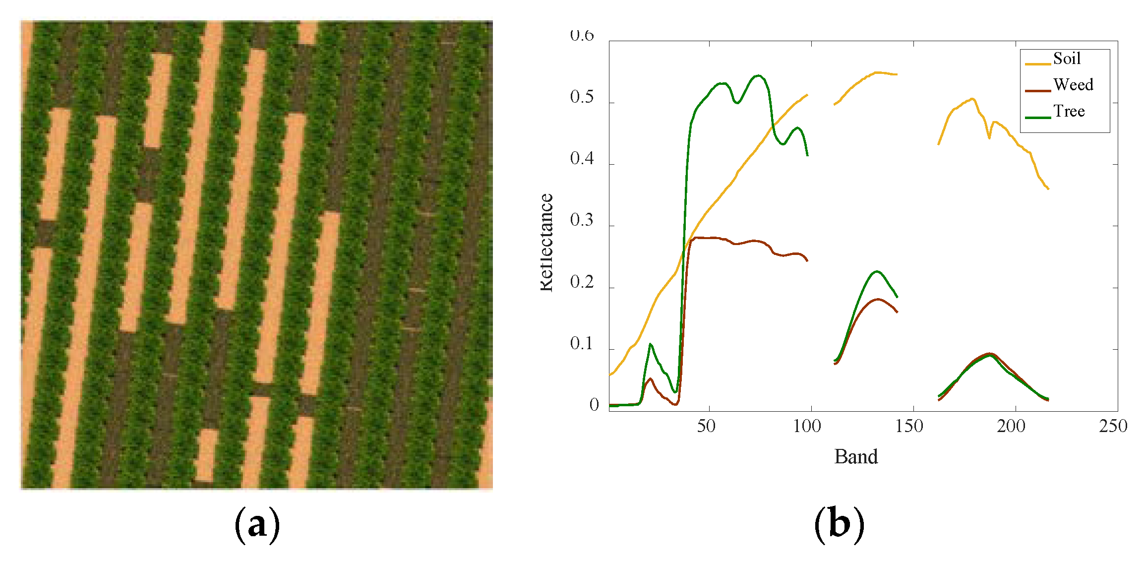
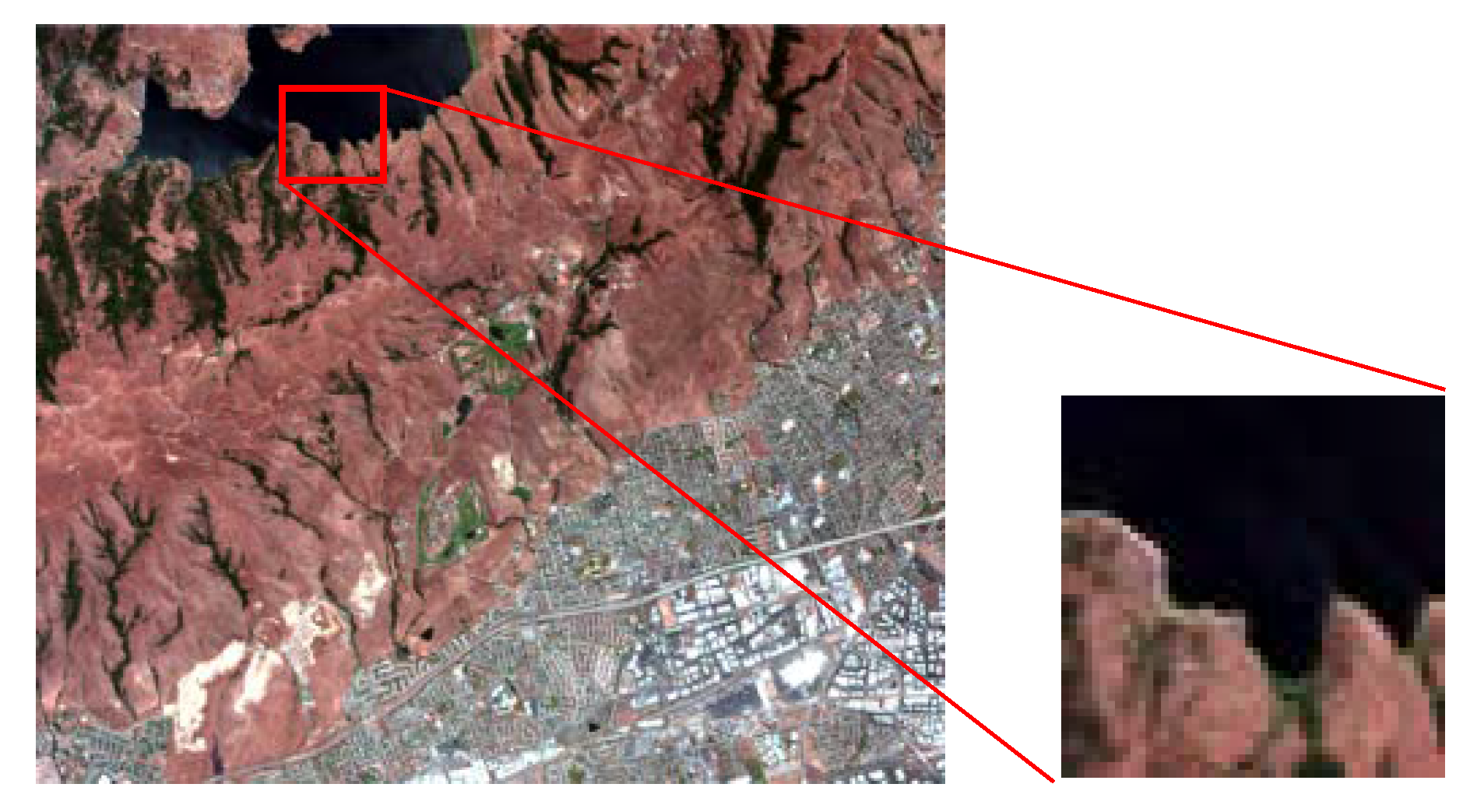
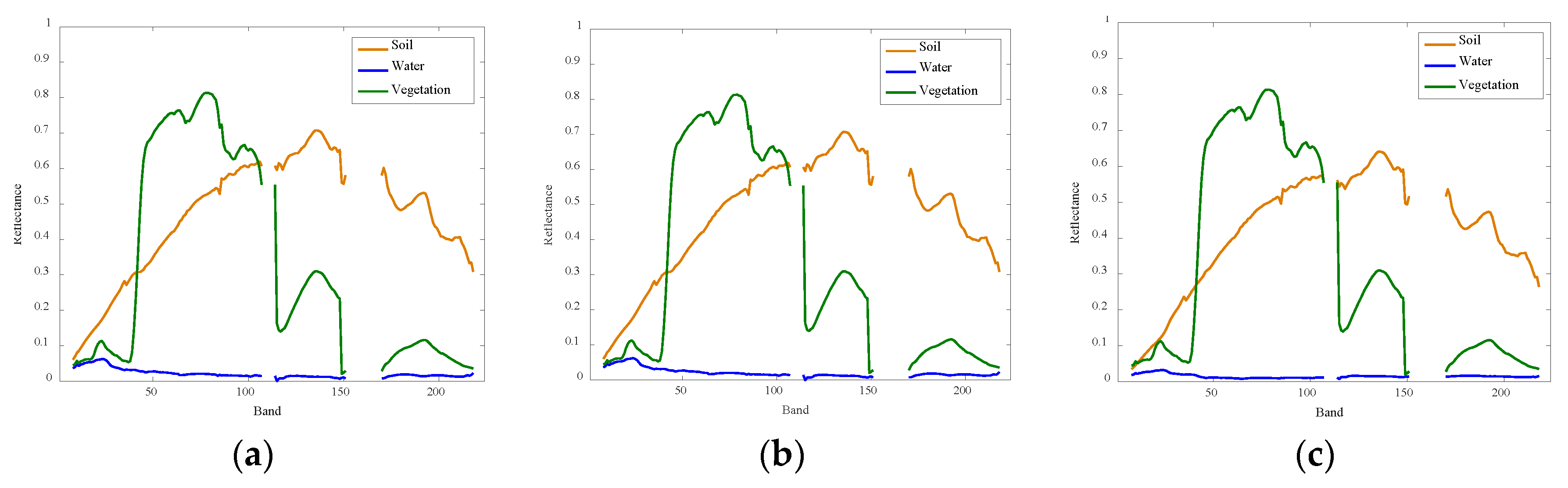
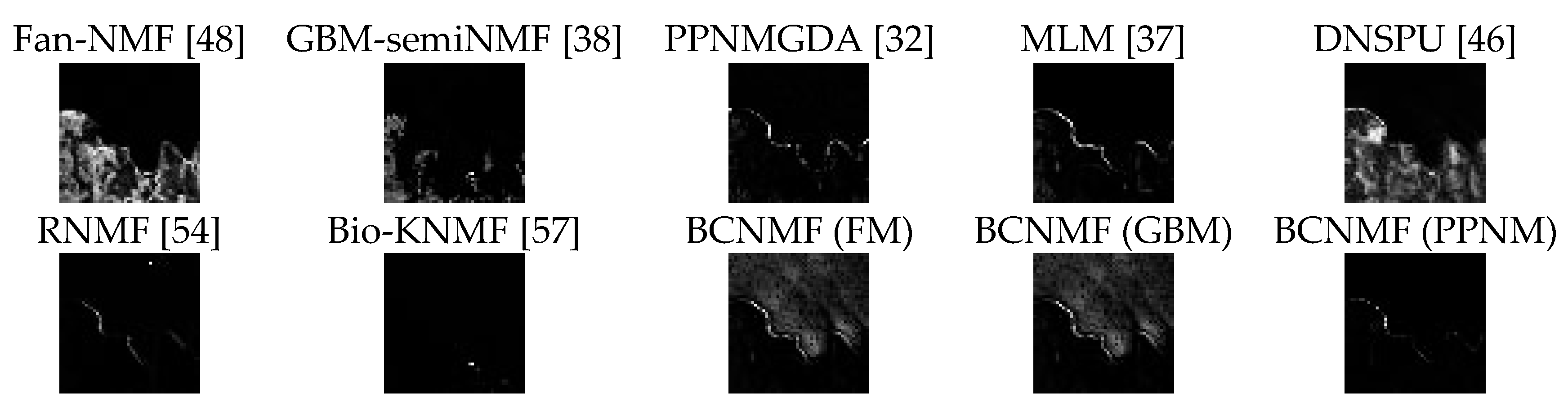
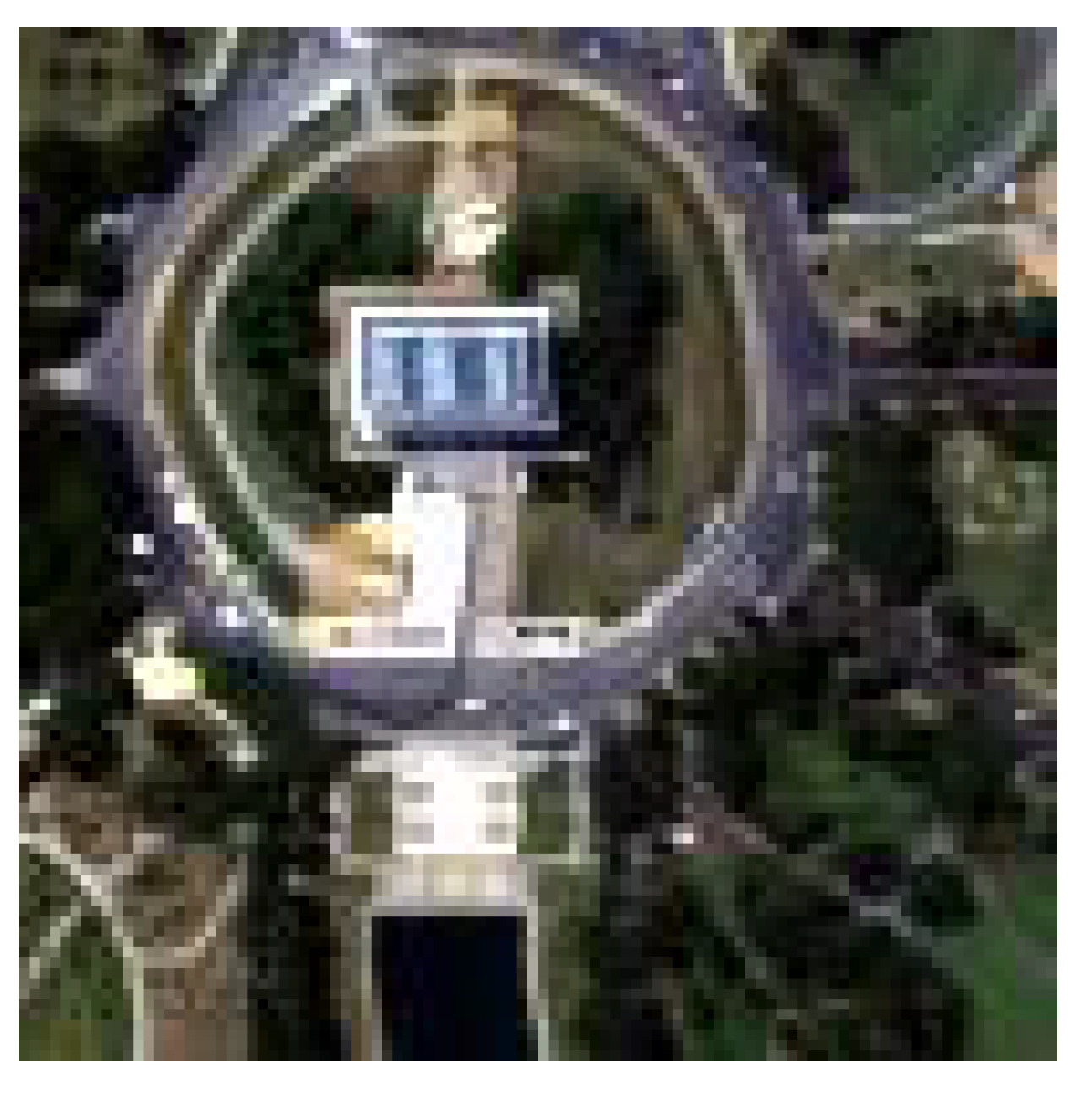
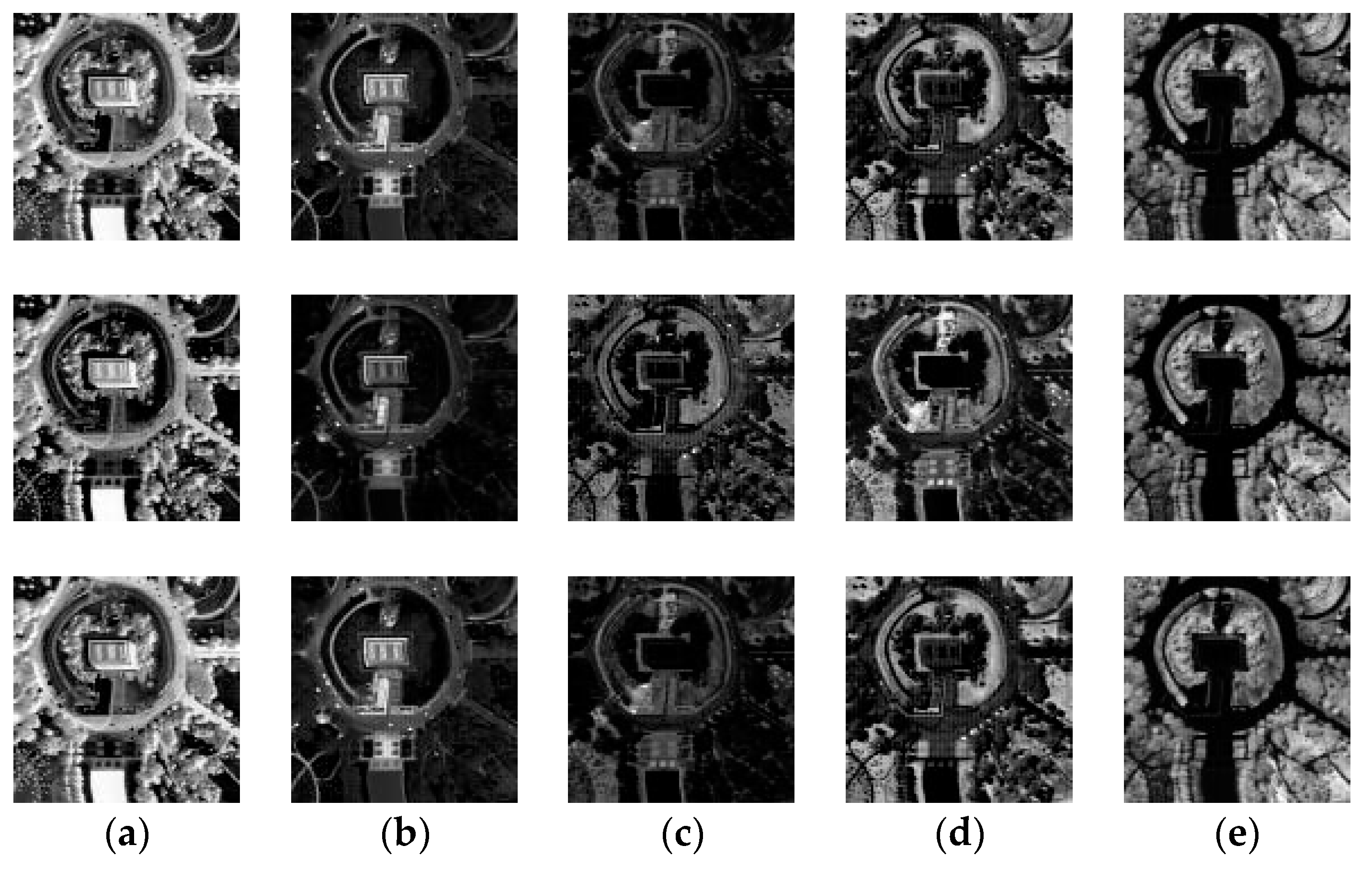
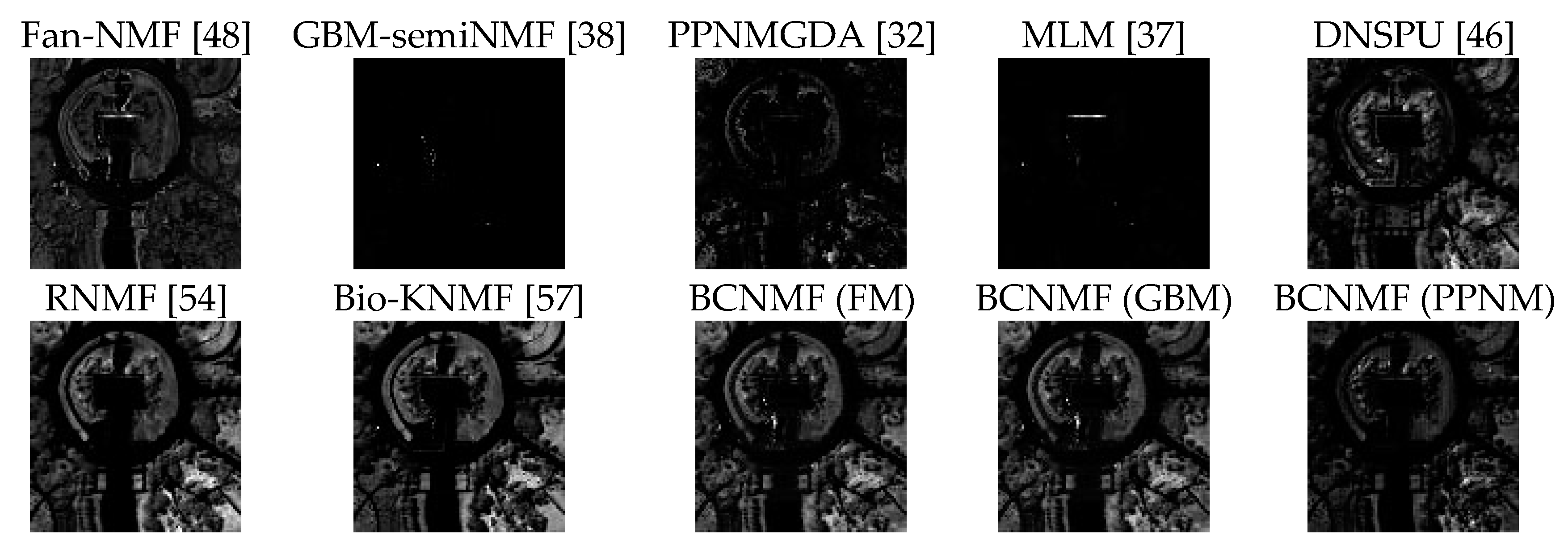
4.2. Experiments with Virtual Orchard and Real Hyperspectral Images

A quasi-real hyperspectral data of virtual citrus orchard constituted by soil, weed, and trees (see Figure 12a) [33,34,70] is first used for evaluation. It is simulated by an extended physically based ray-tracing (PBRT) model [70] so that detailed light-rays’ transmission paths are known, and multiple scattering effects can be modelled realistically. Illumination sources, sensor platforms, geometry descriptions and material optical properties introduced in Table 11 construct the observed scenes. Endmembers’ spectrum in Figure 12b are calibrated through replacing the remaining ground covers with perfectly absorbing background, and averaging those pixels with abundances greater than 0.95 after rendering. This dataset was well calibrated by in situ data, and successfully adopted for evaluating nonlinear unmixing methods recently [34]. The water-vapor absorption bands (99–110, 143–161) were removed in the experiment.
With the use of true endmembers and abundances, quantitative unmixing results are provided in Table 12. The proposed BCNMF under the assumptions of all three BMMs always obtained the best MSADs and RMSEs. In particular, BCNMF based on the PPNM performs much better than other methods. Moreover, it is noted that due to the big similarity of FM and GBM and the use of geometric projection, BCNMF based on these two models obtained the same results. On the other hand, VCA also extracted accurate endmembers because the spatial resolution is high and some pure pixels exist.
Next, the performance of BCNMF is discussed using two well-chosen real hyperspectral images. In the observed areas corresponding to them, ground cover mainly consists of vegetation, soil, and so on, implying that the nonlinear mixing effect may be a non-negligible factor in spectral unmixing [26,27,28,33,34]. Therefore, they are expected to provide a good test for the nonlinear unmixing algorithms. The first image was acquired over Moffett Field, CA, by the Airborne Visible Infrared Imaging Spectrometer (AVIRIS) in 1997. A region of interest (see Figure 13) with a size of 50×50 pixels is selected, and the low SNR bands (1–7, 108–113, 152–169, 219–224) are removed, leaving the remaining 187 bands for the experiment. In fact, this dataset has been widely used for the algorithm evaluation of both linear and nonlinear spectral unmixing in the past [31,32,49,54], the results in the previous works provide the comparison and partial ground truth for the later discussion. Three types of ground cover, including water, soil, and vegetation show a prominent presence in the sub-image of Figure 13.
Since the detailed ground truth is not available, the endmembers’ spectral curves extracted by BCNMF under the FM, GBM, and PPNM are provided in Figure 14, and compare the estimated abundance maps of water, soil, and vegetation in Figure 15 according to the previous results [31,32,49,54]. It can be observed from Figure 14 that three endmembers have been determined well by BCNMF, and approach the real situations no matter what specific BMM is used. Moreover, abundance maps in Figure 15 also display the similarity of the three materials’ distributions to the published results and ground truth. In order to compare the unmixing results of BCNMF with other algorithms’ and analyze the contribution of nonlinearity, the maps of differences between the images reconstructed by the FCLS and other nonlinear spectral unmixing algorithms are further provided in Figure 16. Pixels that are located on the boundary between water and soil (or vegetation) can be easily observed in the corresponding results of BCNMF. Residual errors in these pixels are larger because of the nonlinear mixing effect that has been effectively addressed in the proposed algorithm. Other algorithms such as the PPNMGDA and RNMF also show good performances, but the Fan-NMF, DNSPU and Bio-KNMF seem to be less robust for this dataset. SRE L M M obtained by BCNMF with respect to this dataset is shown in Table 12. Similar to the other nonlinear unmixing methods such as PPNMGDA and MLM, obvious nonlinear components may be quantitatively reflected.
The second image corresponds to a sub-region of the dataset collected by the Hyperspectral Digital Imagery Collection Experiment (HYDICE) sensor over the Mall in Washington DC. After removing the bands affected badly by noise and water absorption bands from the original dataset (210 bands), 100 × 100 pixels with 191 bands comprise the image for the experiment shown in Figure 17. According to the report in [71] and the number of endmembers estimated by HySime [72], five materials including the roofs, trees, water, roads, and grass are considered to be distributed in this area. Due to the limited space, only abundance maps estimated by BCNMF are shown in Figure 18, and Table 12 shows the corresponding SRE L M M of each algorithm. Five materials have been determined and can be easily distinguished from each other. It can be seen that trees and grass occupy the largest area in the image, and the nonlinear mixing effect is supposed to reach a high level between these two materials. Therefore, the differences between the trees’ abundances estimated by the FCLS and other algorithms are further compared in Figure 19. The fact that residual errors of trees’ abundances increase in the area covered by both trees and grass is reflected by BCNMF as well.

5. Discussion

In Section 4, both qualitative and quantitative evaluation of BCNMF and the compared algorithms are presented in the experiments with synthetic data, virtual orchard data and real hyperspectral remote sensing images. The comprehensive results can be very useful to validate BCNMF’s superiority in unsupervised nonlinear unmixing.

5.1. Unmixing Accuracy Improvement by Addressing the Collinearity

Endmembers’ VIFs in Table 2 partly reflect that virtual endmembers can greatly increase the collinearity’s negative influence in nonlinear unmixing. However, this issue can be well addressed by the proposed BCNMF. It is mainly because that the procedure of geometric projection in Equations (5)–(11) can prevent virtual endmembers from participating directly in the abundance estimation. In this process, pixels’ approximate linear components can be obtained, and then nonlinear unmixing is naturally transformed into the linear unmixing. Therefore, the impact of collinearity is significantly reduced and the unmixing accuracy is improved in the proposed method. Nevertheless, traditional algorithms such as Fan-NMF and PPNMGDA which rely on virtual endmembers for the parameter estimation will definitely suffer from the collinearity, resulting in larger unmixing errors.
This viewpoint can be demonstrated by the results in Table 3 where true endmembers are assumed to be known in advance. In this ideal situation, BCNMF shows better or competitive performance, even if the projection coordinates (without any iterations) are directly adopted as the abundances for comparison. We consider that the strong interference of virtual endmembers in unmixing is effectively avoided because of the geometric projection. Moreover, it also implies that the impact of projection bias seems to be weaker than the collinearity in most cases, partly leading to a reasonable explanation of removing the de-biasing process in BCNMF. However, in the case of other compared algorithms, the collinearity might affect seriously the abundance estimation, which cannot be actually addressed by multiple iterations. Since the collinearity problem can be overcome, BCNMF still keeps its outstanding unmixing performance in other experiments where more complex data (e.g., more endmembers and lower SNRs) are considered. Quantitative results including endmembers’ MSADs and abundances’ RMSEs in Table 4, Table 5, Table 6, Table 7, Table 8 and Table 9 prove reasonably that BCNMF is a robust and stable unsupervised nonlinear unmixing algorithm.
Further, the proposed BCNMF is also validated in the experiments with a virtual orchard dataset and two real hyperspectral images. Since true endmembers and abundances in the real hyperspectral data are unknown, the virtual orchard physical-based dataset can be very useful for the quantitative analysis. In Table 12, BCNMF has smaller RMSEs and MSADs than the other algorithms based on the same BMMs, which indicates that it can obtain more accurate endmembers and abundances in this quasi-real situation. In addition, the quantitative SRE L M M with respect to the real data in Table 12 and Figure 14, Figure 15, Figure 16, Figure 17, Figure 18 and Figure 19 further illustrate that BCNMF is able to reflect the nonlinear components in practice like other state-of-the-art methods (e.g., MLM). As stated earlier, we can also infer that the improvement of accuracy in BCNMF mainly comes from the operation of geometric projection which decreases the negative effect of collinearity.

5.2. Improvement of Endmember Extraction for Highly Mixed Nonlinear Data

Endmembers may be wrongly extracted by methods such as VCA especially when pixels are highly mixed. The accuracy of the used endmembers can also influence the geometric projection. Therefore, using the calculated pixels’ approximate linear components, NMF is further exploited in BCNMF to update endmembers and abundances in an unsupervised way. In addition, a minimum-endmember-distance constraint is incorporated into the framework of NMF to produce better unmixing results.
Table 8 and Table 9 show the algorithms’ sensitivities to the degree of mixing. BCNMF extracted the most accurate endmembers no matter when the pixels were highly mixed or not. Besides, more accurate abundances were also obtained by BCNMF. However, VCA failed to extract endmembers accurately, especially when data was highly mixed. As a result, supervised methods (i.e., PPNMGDA, GBM-semiNMF and MLM) using endmembers extracted by VCA could not obtain the abundances as accurate as the results they produced when true endmembers were used in Table 3. Moreover, other unsupervised NMF-based methods still could not outperform the proposed method. It is because that the minimum distance constraint had alleviated the issue of local minima, and enabled BCNMF to find accurate endmembers for data in different mixing degrees. The sensitivity analysis on regularization parameter λ in Figure 11 further proves the necessity of this constraint. When the EMD in Equation (12) is ignored (i.e., λ = 0 ), although RMSEs of the estimated abundances seem not to be influenced, MSADs of the estimated endmembers are always worse than the case λ = 0.1 for all three BMMs. Therefore, we can conclude that BCNMF could find more accurate endmembers compared with other supervised or unsupervised unmixing algorithms, resulting from the incorporation of minimum distance constraint in the NMF framework.
Moreover, Figure 10 proves that BCNMF has a good convergence for nonlinear unmixing. Table 10 further illustrates that the time cost of BCNMF is much lower than the algorithms like PPNMGDA and kernel-based Bio-KNMF. In comparison with the fast methods such as GBM-semiNMF and RNMF, BCNMF’s computational speed can also be slightly better. We consider that the speed advantage of the proposed method should come from both the low computational complexities of geometric projection and constrained NMF.

5.3. Limitations

The combination of geometric projection and minimum distance constrained NMF enables BCNMF to alleviate the collinearity and unmix highly mixed nonlinear hyperspectral data. However, the following limitations should be overcome. (1) An effective scheme may be built to reduce the complexity of de-biasing so that projection bias can be further removed to get better unmixing results; (2) It is noted that we only exploited the geometric characteristics of BMM data without considering the spatial information of hyperspectral imagery. Therefore, a proper spatial regularizer should be adopted in the framework of BCNMF to improve unmixing performance.

6. Conclusions

This paper has presented an unsupervised nonlinear spectral unmixing algorithm by exploiting the common geometric property of BMMs. Through a process of geometric projection, pixels’ approximate linear mixture components are obtained, and then put into the framework of CNMF for further unmixing. Using the given endmembers, pixels’ projections are obtained by a signed distance measure for calculating pixels’ barycentric coordinates on the constructed simplices. As a result, not only the negative effect of collinearity can be overcome, but unsupervised linear spectral unmixing algorithms such as CNMF can also be used to unmix the projections and update endmembers and abundances. Similar to the linear case, the objective function of standard NMF is properly constrained to mitigate the problem of local minima by the endmember distance constraint. After endmembers are updated, projections will be updated as well until the algorithm converges. Compared with the traditional and state-of-the-art algorithms in the experiments with both synthetic data and real hyperspectral images, the proposed algorithm has provided more accurate unmixing results.
In the future work, we will deal with the drawbacks of the proposed method in ignoring projection bias and spatial information of hyperspectral remote sensing imagery. Moreover, an implicit assumption of the BMMs at present is that the strength of nonlinearity in different spectral bands is the same, which is commonly not the case in practical applications. Therefore, a study on the band-wise nonlinear spectral unmixing algorithms will also be an interesting and meaningful piece of work.

Author Contributions

B.Y. conceived and designed the method and experiments, performed the experiments, analyzed the data and wrote the paper. B.W. reviewed the results, edited the paper and provided advices for the preparation and revision of the paper. Z.W. provided the mathematical expertise of this work.

Acknowledgments

The authors would like to thank Dobigeon for sharing the PPNMM-GDA code and simulated data of virtual orchard, Heylen for sharing the DNSPU and MLM code, Févotte for sharing the RNMF code, and Zhu for providing the Bio-KNMF code. This work was supported by the National Natural Science Foundation of China under Grant No. 61572133 and by the Research Fund for the State Key Laboratory of Earth Surface Processes and Resource Ecology under Grant 2017-KF-19.

Conflicts of Interest

The authors declare no conflicts of interest. The founding sponsors had no role in the design of the study; in the collection, analyses, or interpretation of data; in the writing of the manuscript; and in the decision to publish the results.

References

  1. Keshava, N.; Mustard, J.F. Spectral unmixing. IEEE Signal Process. Mag. 2002, 19, 44–57. [Google Scholar] [CrossRef]
  2. Bioucas-Dias, J.M.; Plaza, A.; Dobigeon, N.; Parente, M.; Du, Q.; Gader, P.; Chanussot, J. Hyperspectral unmixing overview: Geometrical, statistical, and sparse regression-based approaches. IEEE J. Sel. Top. Appl. Earth Obs. Remote Sens. 2012, 5, 354–379. [Google Scholar] [CrossRef]
  3. Winter, M.E. N-FINDR: An algorithm for fast autonomous spectral end-member determination in hyperspectral data. In Proceedings of the SPIE’s International Symposium on Optical Science, Engineering, and Instrumentation, San-Diego, CA, USA, 9–14 July 1999. [Google Scholar]
  4. Nascimento, J.M.; Dias, J.M. Vertex component analysis: A fast algorithm to unmix hyperspectral data. IEEE Trans. Geosci. Remote Sens. 2005, 43, 898–910. [Google Scholar] [CrossRef]
  5. Tao, X.; Wang, B.; Zhang, L. Orthogonal bases approach for the decomposition of mixed pixels in hyperspectral imagery. IEEE Geosci. Remote Sens. Lett. 2009, 6, 219–223. [Google Scholar]
  6. Heinz, D.C.; Chang, C.I. Fully constrained least squares linear spectral mixture analysis method for material quantification in hyperspectral imagery. IEEE Trans. Geosci. Remote Sens. 2001, 39, 529–545. [Google Scholar] [CrossRef]
  7. Wang, L.; Liu, D.; Wang, Q. Geometric method of fully constrained least squares linear spectral mixture analysis. IEEE Trans. Geosci. Remote Sens. 2013, 51, 3558–3566. [Google Scholar] [CrossRef]
  8. Chan, T.H.; Chi, C.Y.; Huang, Y.M.; Ma, W.K. A convex analysis based minimum-volume enclosing simplex algorithm for hyperspectral unmixing. IEEE Trans. Signal Process. 2009, 57, 4418–4432. [Google Scholar] [CrossRef]
  9. Lin, C.H.; Cin, C.Y.; Wang, Y.H.; Chan, T.H. A fast hyperplane-based minimum-volume enclosing simplex algorithm for blind hyperspectral unmixing. IEEE Trans. Signal Process. 2016, 64, 1946–1961. [Google Scholar] [CrossRef]
  10. Li, J.; Agathos, A.; Zaharie, D.; Bioucas-Dias, J.M.; Plaza, A.; Li, X. Minimum volume simplex analysis: A fast algorithm for linear hyperspectral unmixing. IEEE Trans. Geosci. Remote Sens. 2015, 53, 5067–5082. [Google Scholar]
  11. Miao, L.; Qi, H. Endmember extraction from highly mixed data using minimum volume constrained nonnegative matrix factorization. IEEE Trans. Geosci. Remote Sens. 2007, 45, 765–777. [Google Scholar] [CrossRef]
  12. Yu, Y.; Guo, S.; Sun, W. Minimum distance constrained nonnegative matrix factorization for the endmember extraction of hyperspectral images. In Proceedings of the SPIE’s Conference on Remote Sensing and GIS Data Processing and Applications, Wuhan, China, 4 November 2007; Volume 6790, pp. 151–159. [Google Scholar]
  13. Lee, D.D.; Seung, H.S. Learning the parts of objects by nonnegative matrix factorization. Nature 1999, 401, 788–791. [Google Scholar] [PubMed]
  14. Schachtner, R.; Pöppel, G.; Tomé, A.M.; Lang, E.W. Minimum determinant constraint for non-negative matrix factorization. In Proceedings of the 8th International Conference on Independent Component Analysis and Signal Separation, Paraty, Brazil, 15–18 March 2009; pp. 106–113. [Google Scholar]
  15. Wang, N.; Du, B.; Zhang, L. An endmember dissimilarity constrained non-negative matrix factorization method for hyperspectral unmixing. IEEE J. Sel. Top. Appl. Earth Obs. Remote Sens. 2013, 6, 554–569. [Google Scholar] [CrossRef]
  16. Liu, X.; Xia, W.; Wang, B.; Zhang, L. An approach based on constrained nonnegative matrix factorization to unmix hyperspectral data. IEEE Trans. Geosci. Remote Sens. 2011, 49, 757–772. [Google Scholar] [CrossRef]
  17. Jia, S.; Qian, Y. Constrained nonnegative matrix factorization for hyperspectral unmixing. IEEE Trans. Geosci. Remote Sens. 2009, 47, 161–173. [Google Scholar] [CrossRef]
  18. Yang, S.; Zhang, X.; Yao, Y.; Cheng, S.; Jiao, L. Geometric nonnegative matrix factorization (GNMF) for hyperspectral unmixing. IEEE J. Sel. Top. Appl. Earth Obs. Remote Sens. 2015, 8, 2696–2703. [Google Scholar] [CrossRef]
  19. Tong, L.; Zhou, J.; Li, X.; Qian, Y.; Gao, Y. Region-based structure preserving nonnegative matrix factorization for hyperspectral unmixing. IEEE J. Sel. Top. Appl. Earth Obs. Remote Sens. 2017, 10, 1575–1588. [Google Scholar] [CrossRef]
  20. Qian, Y.; Jia, S.; Zhou, J.; Robles-Kelly, A. Hyperspectral unmixing via L1/2 sparsity-constrained nonnegative matrix factorization. IEEE Trans. Geosci. Remote Sens. 2011, 49, 4282–4297. [Google Scholar] [CrossRef]
  21. Lu, X.; Wu, H.; Yuan, Y.; Yan, P.; Li, X. Manifold regularized sparse NMF for hyperspectral unmixing. IEEE Trans. Geosci. Remote Sens. 2013, 51, 2815–2826. [Google Scholar] [CrossRef]
  22. Wang, W.; Qian, Y.; Tang, Y. Hypergraph-regularized sparse NMF for hyperspectral unmixing. IEEE J. Sel. Top. Appl. Earth Obs. Remote Sens. 2016, 9, 681–694. [Google Scholar] [CrossRef]
  23. He, W.; Zhang, H.; Zhang, L. Sparsity-regularized robust non-negative matrix factorization for hyperspectral unmixing. IEEE J. Sel. Top. Appl. Earth Obs. Remote Sens. 2016, 9, 4267–4279. [Google Scholar] [CrossRef]
  24. Yuan, Y.; Fu, M.; Lu, X. Substance dependence constrained sparse NMF for hyperspectral unmixing. IEEE Trans. Geosci. Remote Sens. 2015, 53, 2975–2986. [Google Scholar] [CrossRef]
  25. Li, J.; Bioucas-Dias, J.M.; Plaza, A.; Liu, L. Robust collaborative nonnegative matrix factorization for hyperspectral unmixing. IEEE Trans. Geosci. Remote Sens. 2016, 54, 6076–6090. [Google Scholar] [CrossRef]
  26. Dobigeon, N.; Tourneret, J.Y.; Richard, C.; Bermudez, J.C.; McLaughlin, S.; Hero, A.O. Nonlinear unmixing of hyperspectral images: Models and algorithms. IEEE Signal Process. Mag. 2014, 31, 82–94. [Google Scholar] [CrossRef]
  27. Heylen, R.; Parente, M.; Gader, P. A review of nonlinear hyperspectral unmixing methods. IEEE J. Sel. Top. Appl. Earth Obs. Remote Sens. 2014, 7, 1844–1868. [Google Scholar] [CrossRef]
  28. Mustard, J.F.; Pieters, C.M. Quantitative abundance estimates from bidirectional reflectance measurements. J. Geophys. Res. Solid Earth 1987, 92, E617–E626. [Google Scholar] [CrossRef]
  29. Hapke, B. Bidirection reflectance spectroscopy. I. theory. J. Geophys. Res. 1981, 86, 3039–3054. [Google Scholar] [CrossRef]
  30. Fan, W.; Hu, B.; Miller, J.; Li, M. Comparative study between a new nonlinear model and common linear model for analysing laboratory simulated-forest hyperspectral data. Int. J. Remote Sens. 2009, 30, 2951–2962. [Google Scholar] [CrossRef]
  31. Halimi, A.; Altmann, Y.; Dobigeon, N.; Tourneret, J.Y. Nonlinear unmixing of hyperspectral images using a generalized bilinear model. IEEE Trans. Geosci. Remote Sens. 2011, 49, 4153–4162. [Google Scholar] [CrossRef] [Green Version]
  32. Altmann, Y.; Halimi, A.; Dobigeon, N.; Tourneret, J.Y. Supervised nonlinear spectral unmixing using a postnonlinear mixing model for hyperspectral imagery. IEEE Trans. Image Process. 2012, 21, 3017–3025. [Google Scholar] [CrossRef] [PubMed] [Green Version]
  33. Somers, B.; Tits, L.; Coppin, P. Quantifying nonlinear spectral mixing in vegetated areas: Computer simulation model validation and first results. IEEE J. Sel. Top. Appl. Earth Obs. Remote Sens. 2014, 7, 1956–1965. [Google Scholar] [CrossRef]
  34. Dobigeon, N.; Tits, L.; Somers, B.; Altmann, Y.; Coppin, P. A comparison of nonlinear mixing models for vegetated areas using simulated and real hyperspectral data. IEEE J. Sel. Top. Appl. Earth Obs. Remote Sens. 2014, 7, 1869–1878. [Google Scholar] [CrossRef]
  35. Marinoni, A.; Gamba, P. A novel approach for efficient p-linear hyperspectral unmixing. IEEE J. Sel. Top. Signal Process. 2015, 9, 1156–1168. [Google Scholar] [CrossRef]
  36. Halimi, A.; Bioucas-Dias, J.M.; Dobigeon, N.; Buller, G.S.; McLaughlin, S. Fast hyperspectral unmixing in presence of nonlinearity or mismodeling effects. IEEE Trans. Comput. Imaging 2017, 3, 146–159. [Google Scholar] [CrossRef]
  37. Heylen, R.; Scheunders, P. A multilinear mixing model for nonlinear spectral unmixing. IEEE Trans. Geosci. Remote Sens. 2016, 54, 240–251. [Google Scholar] [CrossRef]
  38. Yokoya, N.; Chanussot, J.; Iwasaki, A. Nonlinear unmixing of hyperspectral data using semi-nonnegative matrix factorization. IEEE Trans. Geosci. Remote Sens. 2014, 52, 1430–1437. [Google Scholar] [CrossRef]
  39. Pu, H.; Chen, Z.; Wang, B.; Xia, W. Constrained least squares algorithms for nonlinear unmixing of hyperspectral imagery. IEEE Trans. Geosci. Remote Sens. 2015, 53, 1287–1303. [Google Scholar] [CrossRef]
  40. Li, C.; Ma, Y.; Huang, J.; Mei, X.; Liu, C.; Ma, J. GBM-based unmixing of hyperspectral data using bound projected optimal gradient method. IEEE Geosci. Remote Sens. Lett. 2016, 13, 952–956. [Google Scholar] [CrossRef]
  41. Chen, J.; Richard, C.; Honeine, P. Nonlinear estimation of material abundances in hyperspectral images with l1-norm spatial regularization. IEEE Trans. Geosci. Remote Sens. 2013, 52, 2654–2665. [Google Scholar] [CrossRef]
  42. Qu, Q.; Nasrabadi, N.M.; Tran, T.D. Abundance estimation for bilinear mixture models via joint sparse and low-rank representation. IEEE Trans. Geosci. Remote Sens. 2014, 52, 4404–4423. [Google Scholar]
  43. Li, J.; Li, X.; Huang, B.; Zhao, L. Hopfield neural network approach for supervised nonlinear spectral unmixing. IEEE Geosci. Remote Sens. Lett. 2016, 13, 1002–1006. [Google Scholar] [CrossRef]
  44. Broadwater, J.; Chellappa, R.; Banerjee, A.; Burlina, P. Kernel fully constrained least squares abundance estimates. In Proceedings of the IEEE Geoscience and Remote Sensing Symposium, Barcelona, Spain, 23–28 July 2007; pp. 4041–4044. [Google Scholar]
  45. Chen, J.; Richard, C.; Honeine, P. Nonlinear unmixing of hyperspectral data based on a linear mixture/nonlinear-fluctuation model. IEEE Trans. Signal Process. 2013, 61, 480–492. [Google Scholar] [CrossRef]
  46. Heylen, R.; Scheunders, P. A distance geometric framework for nonlinear hyperspectral unmixing. IEEE J. Sel. Top. Appl. Earth Obs. Remote Sens. 2014, 7, 1879–1888. [Google Scholar] [CrossRef]
  47. Altmann, Y.; Dobigeon, N.; Tourneret, J.Y. Unsupervised post-nonlinear unmixing of hyperspectral images using a Hamiltonian Monte Carlo algorithm. IEEE Trans. Image Process. 2014, 23, 2663–2675. [Google Scholar] [CrossRef] [PubMed] [Green Version]
  48. Eches, O.; Guillaume, M. A bilinear-bilinear nonnegative matrix factorization method for hyperspectral unmixing. IEEE Geosci. Remote Sens. Lett. 2014, 11, 778–782. [Google Scholar] [CrossRef]
  49. Luo, W.; Gao, L.; Plaza, A.; Marinoni, A.; Yang, B.; Zhong, L.; Gamba, P.; Zhang, B. A new algorithm for bilinear spectral unmixing of hyperspectral images using particle swarm optimization. IEEE J. Sel. Top. Appl. Earth Obs. Remote Sens. 2016, 9, 5776–5790. [Google Scholar] [CrossRef]
  50. Somers, B.; Cools, K.; Delalieux, S.; Stuckens, J.; Van der Zande, D.; Verstraeten, W.W.; Coppin, P. Nonlinear hyperspectral image analysis for tree cover estimates in orchards. Remote Sens. Environ. 2009, 113, 1183–1193. [Google Scholar] [CrossRef]
  51. Chen, X.; Chen, J.; Jia, X.; Somers, B.; Wu, J.; Coppin, P. A quantitative analysis of virtual endmembers’ increased impact on the collinearity effect in spectral unmixing. IEEE Trans. Geosci. Remote Sens. 2011, 49, 2945–2956. [Google Scholar] [CrossRef]
  52. Ma, L.; Chen, J.; Zhou, Y.; Chen, X. Two-step constrained nonlinear spectral mixture analysis method for mitigating the collinearity effect. IEEE Trans. Geosci. Remote Sens. 2016, 54, 2873–2886. [Google Scholar] [CrossRef]
  53. Van der Meer, F.D.; Jia, X.P. Collinearity and orthogonality of endmembers in linear spectral unmixing. Int. J. Appl. Earth Obs. Geoinf. 2012, 18, 491–503. [Google Scholar] [CrossRef]
  54. Févotte, C.; Dobigeon, N. Nonlinear hyperspectral unmixing with robust nonnegative matrix factorization. IEEE Trans. Image Process. 2015, 24, 4810–4819. [Google Scholar] [CrossRef] [PubMed]
  55. Li, X.; Cui, J.; Zhao, L. Blind nonlinear hyperspectral unmixing based on constrained kernel nonnegative matrix factorization. Signal Image Video Process. 2014, 8, 1555–1567. [Google Scholar] [CrossRef]
  56. Cui, J.; Li, X.; Zhao, L. Nonlinear hyperspectral unmxing based on constrained multiple kernel NMF. In Proceedings of the SPIE’s Satellite Data Compression, Communications, and Processing, Baltimore, MD, USA, 22 May 2014; Volume 9124, pp. N1–N6. [Google Scholar]
  57. Zhu, F.; Honeine, P. Biobjective nonnegative matrix factorization linear versus kernel-based models. IEEE Trans. Geosci. Remote Sens. 2016, 54, 4012–4022. [Google Scholar] [CrossRef]
  58. Yang, B.; Wang, B.; Wu, Z. Nonlinear hyperspectral unmixing based on geometric characteristics of bilinear mixture models. IEEE Trans. Geosci. Remote Sens. 2018, 56, 694–714. [Google Scholar] [CrossRef]
  59. Shen, W. Introduction to the Theory of Simplex: Research on High. Dimensional Extension of Triangle; Hunan Normal University Press: Changsha, China, 2000. [Google Scholar]
  60. Ungar, A. Barycentric Calculus in Euclidean and Hyperbolic Geometry: A Comparative Introduction; World Scientific: Singapore, 2010. [Google Scholar]
  61. Honeine, P.; Richard, C. Geometric unmixing of large hyperspectral images: A barycentric coordinate approach. IEEE Trans. Geosci. Remote Sens. 2011, 50, 2185–2195. [Google Scholar] [CrossRef]
  62. Heylen, R.; Burazerović, D.; Scheunders, P. Fully constrained least squares spectral unmixing by simplex projection. IEEE Trans. Geosci. Remote Sens. 2011, 49, 4112–4122. [Google Scholar] [CrossRef]
  63. Farin, G.; Hoschek, J.; Kim, M.S. Handbook of Computer Aided Geometric Design; Elsevier: Amsterdam, The Netherlands, 2002. [Google Scholar]
  64. Strang, G. Linear Algebra and Its Applications, 4th ed.; Thomson: Belmont, CA, USA, 2006. [Google Scholar]
  65. Boyd, S.; Vandenberghe, L. Convex Optimization; Cambridge University Press: Cambridge, UK, 2004. [Google Scholar]
  66. Lin, I.H. Geometric Linear Algebra; World Scientific: Singapore, 2008. [Google Scholar]
  67. Yang, B.; Wang, B.; Wu, Z.; Lu, Q. Bilinear mixture models based unsupervised nonlinear unmixing using constrained nonnegative matrix factorization. In Proceedings of the 2017 IEEE International Geoscience and Remote Sensing Symposium (IGARSS), Fort Worth, TX, USA, 23–28 July 2017; pp. 582–585. [Google Scholar]
  68. Lin, C.J. Projected gradient methods for non-negative matrix factorization. Neural Comput. 2007, 19, 2756–2777. [Google Scholar] [CrossRef] [PubMed]
  69. Iordache, M.; Bioucas-Dias, J.M.; Plaza, A. Sparse unmixing of hyperspectral data. IEEE Trans. Geosci. Remote Sens. 2011, 49, 2014–2039. [Google Scholar] [CrossRef]
  70. Stuckens, J.; Somers, B.; Delalieux, S.; Verstraeten, W.W.; Coppin, P. The impact of common assumptions on canopy radiative transfer simulations: A case study in citrus orchards. J. Quant. Spectrosc. Radiat. Transf. 2009, 110, 1–21. [Google Scholar] [CrossRef]
  71. Bethel, J.S.; Lee, C.; Landgrebe, D.A. Geometric registration and classification of hyperspectral airborne pushbroom data. Int. Arch. Photogramm. Remote Sens. 2000, 33, 183–190. [Google Scholar]
  72. Bioucas-Dias, J.M.; Nascimento, J.M. Hyperspectral subspace identification. IEEE Trans. Geosci. Remote Sens. 2008, 46, 2435–2445. [Google Scholar] [CrossRef]
Figure 1. Geometric distribution of the data according to each model described by the three most significant principle components (PCs): (a) linear mixture model (LMM); (b) Fan model FM; (c) generalized bilinear model (GBM); (d) polynomial post-nonlinear model (PPNM).
Remotesensing 10 00801 g001
Figure 2. An example of virtual endmember’s spectral curve.
Remotesensing 10 00801 g002
Figure 3. Geometric interpretation of Property 1. x is a BMM pixel, y is x ’s projection on the line of two endmembers a 1 and a 2 . If p lies on the line of x and its linear mixture component x L M M = a 1 s 1 + a 2 s 2 , y has the same abundances with respect to a1 and a2 as x [59,60,61,62] (i.e., y = xLMM). The case can be extended to a high-dimensional space as well.
Remotesensing 10 00801 g003
Figure 4. Illustration of projection in the feature subspace. (a) construction of the nonlinear vertex p ; (b) geometric distance measure-based projection using nonlinear planes.
Remotesensing 10 00801 g004
Figure 5. Endmember extraction for highly-mixed FM data.
Remotesensing 10 00801 g005
Figure 6. The impact of the accuracy of endmembers on projections: (a) true endmembers; (b) vertex component analysis (VCA) endmembers.
Remotesensing 10 00801 g006
Figure 7. Flowchart of the proposed method.
Remotesensing 10 00801 g007
Figure 8. Diagram of geometric projection onto hyperplanes. (a) LMM; (b) bilinear mixture models (BMMs).
Remotesensing 10 00801 g008
Figure 9. Endmember spectra. (a) Maple_Leaves DW92-1; (b) Olivine GDS70.a Fo89 165 um; (c) Calcite CO2004; (d) Quartz GDS74 Sand Ottawa; (e) Grass_dry.9+.1green AMX32; (f) Muscovite GDS107; (g) Alunite GDS82 Na82; (h) Uralite HS345.3B; (i) Mascagnite GDS65.a.
Remotesensing 10 00801 g009
Figure 10. Convergence analysis of BMM-based constrained NMF algorithm (BCNMF): (a) MSADs; (b) RMSEs.
Remotesensing 10 00801 g010
Figure 11. The unmixing accuracies of BCNMF when regularization parameter λ changes: (a) MSADs; (b) RMSEs.
Remotesensing 10 00801 g011
Figure 12. Virtual orchard dataset [34]: (a) high-resolution image (tree, soil and weed); (b) endmembers’ spectral curves.
Remotesensing 10 00801 g012
Figure 13. Region of interest in the Airborne Visible Infrared Imaging Spectrometer (AVIRIS) Moffett image.
Remotesensing 10 00801 g013
Figure 14. Endmembers extracted by BCNMF based on three BMMs: (a) FM; (b) GBM; (c) PPNM.
Remotesensing 10 00801 g014
Figure 15. Abundance maps of AVIRIS data estimated by BCNMF.
Remotesensing 10 00801 g015
Figure 16. The differences in reconstructed images between the FCLS and nonlinear spectral unmixing algorithms.
Remotesensing 10 00801 g016
Figure 17. Sub-region of Hyperspectral Digital Imagery Collection Experiment (HYDICE) data.
Remotesensing 10 00801 g017
Figure 18. Abundance maps of HYDICE data estimated by BCNMF based on the FM, GBM, and PPNM, respectively, from top row to bottom row. Each column corresponds to the abundances of five endmembers: (a) water; (b) roofs; (c) roads; (d) grass; (e) trees.
Remotesensing 10 00801 g018
Figure 19. The differences in trees’ abundance maps between the fully constrained least squares (FCLS) and nonlinear spectral unmixing algorithms.
Remotesensing 10 00801 g019
Table 1. Parameters of different mixture models.
Models t 1 t 2 b i , k , j
LMM [1] 0
FM [30] r 1 i + 1 1
GBM [31] r 1 i + 1 0 γ i , k , j 1
PPNM [32] r 1 ξ j
Table 2. Comparison of minimum variance inflation factors (VIFs) under different numbers of endmembers.
Number of EndmembersTrue EndmembersTrue and Virtual Endmembers
35.15191.6
519.5113,198.5
721.2253,791.4
921.9882,106.4
Table 3. Root mean square errors (RMSEs) of all algorithms with different numbers of true endmembers (supervised).
ModelsNumber of EndmembersFCLS [6]FanNMF [48]GBMsemiNMF [38]PPNMGDA [32]MLM [37]DNSPU [46]RNMF [54]Bio-KNMF [57]BCNMF
RMSEFM30.0611 ± 0.00000.0110 ± 0.00000.0322 ± 0.00010.0297 ± 0.00010.1042 ± 0.00010.0689 ± 0.00060.0492 ± 0.00050.0731 ± 0.00000.0340 ± 0.0340
50.1132 ± 0.00000.0774 ± 0.00000.0987 ± 0.00010.0186 ± 0.00030.0888 ± 0.00010.1710 ± 0.01260.1081 ± 0.00000.1056 ± 0.00000.0265 ± 0.0265
70.1317 ± 0.00000.0927 ± 0.00000.1161 ± 0.00000.0223 ± 0.00080.1352 ± 0.00000.1719 ± 0.00810.1236 ± 0.00010.1255 ± 0.00000.0194 ± 0.0194
90.1325 ± 0.00000.0973 ± 0.00000.1169 ± 0.00010.0225 ± 0.00110.1285 ± 0.00000.1615 ± 0.01360.1263 ± 0.00020.1285 ± 0.00000.0162 ± 0.0162
GBM30.0345 ± 0.00000.0359 ± 0.00010.0210 ± 0.00010.0192 ± 0.00000.0535 ± 0.00010.0529 ± 0.00070.0298 ± 0.00050.0418 ± 0.00000.0214 ± 0.0000
50.0662 ± 0.00000.0573 ± 0.00000.0587 ± 0.00010.0139 ± 0.00020.0472 ± 0.00010.2003 ± 0.00700.0636 ± 0.00000.0598 ± 0.00010.0179 ± 0.0000
70.0789 ± 0.00000.0637 ± 0.00000.0717 ± 0.00010.0160 ± 0.00030.0732 ± 0.00010.1613 ± 0.00720.0755 ± 0.00010.0754 ± 0.00000.0149 ± 0.0001
90.0806 ± 0.00000.0660 ± 0.00010.0735 ± 0.00010.0158 ± 0.00050.0742 ± 0.00010.1631 ± 0.01150.0779 ± 0.00010.0783 ± 0.00000.0132 ± 0.0001
PPNM30.0594 ± 0.00000.0725 ± 0.00000.0484 ± 0.00010.0029 ± 0.00110.0547 ± 0.00010.0932 ± 0.00040.0730 ± 0.00010.0525 ± 0.00000.0112 ± 0.0000
50.0768 ± 0.00000.0691 ± 0.00000.0652 ± 0.00010.0081 ± 0.00070.0495 ± 0.00010.1975 ± 0.00990.0795 ± 0.00000.0673 ± 0.00000.0146 ± 0.0001
70.0786 ± 0.00000.0739 ± 0.00000.0696 ± 0.00000.0146 ± 0.00060.0621 ± 0.00010.1829 ± 0.01750.0800 ± 0.00010.0705 ± 0.00000.0123 ± 0.0001
90.0727 ± 0.00000.0681 ± 0.00000.0656 ± 0.00000.0156 ± 0.00050.0613 ± 0.00010.1660 ± 0.01660.0734 ± 0.00000.0674 ± 0.00000.0121 ± 0.0001
Table 4. MSADs of all algorithms with different numbers of endmembers.
ModelsNumber of EndmembersVCA [4]Fan-NMF [48]DNSPU [46]RNMF [54]Bio-KNMF [57]BCNMF
MSADFM38.8265 ± 0.35365.2502 ± 0.34739.0515 ± 0.01905.0690 ± 0.29256.8671 ± 0.34212.0462 ± 0.2358
55.6533 ± 0.75415.7124 ± 0.64517.7206 ± 0.44635.1270 ± 1.00046.9426 ± 0.69951.1358 ± 0.0226
75.0358 ± 0.78535.2417 ± 0.42506.6328 ± 0.64474.6294 ± 0.42335.8363 ± 0.35331.4401 ± 0.4295
96.7803 ± 0.48316.7997 ± 0.36738.4783 ± 0.88276.5700 ± 0.67057.0620 ± 0.39642.1292 ± 0.6556
GBM38.0771 ± 0.19515.1468 ± 0.20669.1713 ± 0.36674.9098 ± 0.43386.6004 ± 0.04061.6405 ± 0.1271
55.0001 ± 0.33215.3684 ± 0.24907.0954 ± 0.87664.2958 ± 0.34255.8363 ± 0.21281.0418 ± 0.0545
74.4557 ± 0.68214.4152 ± 0.66576.5340 ± 0.34084.2153 ± 1.12674.8520 ± 0.09950.9470 ± 0.0655
96.5236 ± 0.29476.5768 ± 0.24357.3865 ± 0.38256.2732 ± 0.36156.3688 ± 0.30572.3192 ± 0.0915
PPNM36.8858 ± 0.27604.4980 ± 0.82668.3913 ± 0.37804.6595 ± 0.29086.3666 ± 0.63361.1441 ± 0.3204
54.7601 ± 0.64234.7758 ± 0.45756.9357 ± 0.56774.1588 ± 0.49305.1088 ± 0.30591.0886 ± 0.3378
74.9075 ± 0.49705.2785 ± 0.41489.4223 ± 0.25414.6159 ± 0.46785.5037 ± 0.08721.7113 ± 0.2294
96.1033 ± 0.39876.5077 ± 0.26287.6376 ± 0.27845.8120 ± 0.35076.2541 ± 0.31281.6238 ± 0.1240
Table 5. RMSEs of all algorithms with different numbers of endmembers.
ModelsNumber of EndmembersFCLS (VCA) [6]FanNMF [48]GBMsemiNMF (VCA) [38]PPNMGDA (VCA) [32]MLM (VCA) [37]DNSPU [46]RNMF [54]Bio-KNMF [57]BCNMF
RMSEFM30.0982 ± 0.00420.0623 ± 0.00190.1023 ± 0.00380.0957 ± 0.00890.1398 ± 0.00710.0725 ± 0.00050.0814 ± 0.00380.0949 ± 0.00380.0407 ± 0.0034
50.1294 ± 0.02710.1051 ± 0.01100.1188 ± 0.03070.0862 ± 0.03140.1191 ± 0.02200.1922 ± 0.00920.4016 ± 1.05980.1305 ± 0.03070.0168 ± 0.0002
70.1391 ± 0.02560.1202 ± 0.01540.1259 ± 0.02360.0864 ± 0.02320.1319 ± 0.01640.1719 ± 0.01180.4827 ± 0.95070.1571 ± 0.02360.0137 ± 0.0039
90.1342 ± 0.01900.1333 ± 0.01670.1262 ± 0.01830.1175 ± 0.01850.1350 ± 0.01450.1515 ± 0.00780.3043 ± 0.53740.1407 ± 0.01830.0140 ± 0.0096
GBM30.0984 ± 0.00260.0691 ± 0.00160.0956 ± 0.00520.0856 ± 0.00430.1032 ± 0.00650.0688 ± 0.00260.0824 ± 0.00220.0955 ± 0.00520.0353 ± 0.0021
50.1097 ± 0.03320.1007 ± 0.03230.1033 ± 0.03470.0802 ± 0.02230.0873 ± 0.01790.1963 ± 0.00560.1700 ± 0.18020.0972 ± 0.03470.0166 ± 0.0007
70.0988 ± 0.01420.0940 ± 0.01190.0922 ± 0.01360.0719 ± 0.01340.0966 ± 0.01160.1667 ± 0.01220.0980 ± 0.01510.0967 ± 0.01360.0144 ± 0.0006
90.1405 ± 0.01240.1315 ± 0.01100.1333 ± 0.01300.1246 ± 0.01150.1389 ± 0.00900.1578 ± 0.00740.1440 ± 0.01920.1287 ± 0.01300.0165 ± 0.0320
PPNM30.1328 ± 0.02810.1122 ± 0.02150.1372 ± 0.03850.1018 ± 0.01020.1029 ± 0.01070.1457 ± 0.00130.1164 ± 0.01840.1169 ± 0.03850.0402 ± 0.0060
50.1393 ± 0.01800.1269 ± 0.01560.1289 ± 0.01970.0794 ± 0.01450.0881 ± 0.01840.2021 ± 0.00880.1352 ± 0.01700.1282 ± 0.01970.0290 ± 0.0029
70.1300 ± 0.00780.1246 ± 0.00800.1225 ± 0.00850.0806 ± 0.00910.0964 ± 0.00700.1798 ± 0.01160.1278 ± 0.00780.1302 ± 0.00850.0265 ± 0.0024
90.1317 ± 0.01320.1331 ± 0.01070.1289 ± 0.01250.1059 ± 0.01300.1194 ± 0.01250.1579 ± 0.00850.1341 ± 0.01390.1338 ± 0.01250.0183 ± 0.0010
Table 6. MSADs of all algorithms with different SNRs.
ModelsSNRVCA [4]Fan-NMF [48]DNSPU [46]RNMF [54]Bio-KNMF [57]BCNMF
MSADFM60 dB5.1928 ± 0.83625.1790 ± 0.65287.0513 ± 0.15454.3165 ± 0.36966.0327 ± 0.14600.9740 ± 0.5282
50 dB5.3686 ± 0.82615.6142 ± 0.61426.8207 ± 0.01894.8229 ± 0.60076.2430 ± 0.28021.0818 ± 0.8847
40 dB5.6533 ± 0.75415.7124 ± 0.64517.7206 ± 0.44635.1270 ± 1.00046.9426 ± 0.69951.1358 ± 0.0226
30 dB5.9726 ± 0.81385.4218 ± 0.60518.0765 ± 0.40965.2381 ± 1.20906.4824 ± 0.77231.3058 ± 0.1420
20 dB6.5694 ± 1.20146.1931 ± 0.910511.7315 ± 1.57615.3623 ± 1.39756.3718 ± 0.58302.4998 ± 0.4998
GBM60 dB5.4980 ± 0.53125.7940 ± 0.51426.8903 ± 0.00244.7873 ± 0.72746.4455 ± 0.12320.9570 ± 0.2143
50 dB5.1095 ± 0.86065.1122 ± 0.83006.8639 ± 0.50654.4089 ± 1.07675.8294 ± 0.59110.7909 ± 0.0658
40 dB5.0001 ± 0.33215.3684 ± 0.24907.0954 ± 0.87664.2958 ± 0.34255.8363 ± 0.21281.0418 ± 0.0545
30 dB5.5078 ± 0.90065.7078 ± 0.72909.1409 ± 0.68894.7647 ± 0.88815.9193 ± 0.65450.7008 ± 0.2155
20 dB5.9762 ± 0.82176.0560 ± 0.612112.3400 ± 1.30264.6946 ± 1.07086.8835 ± 0.73003.2856 ± 0.5320
PPNM60 dB4.0249 ± 0.89294.3834 ± 0.32548.3420 ± 0.07423.6025 ± 0.52875.0740 ± 0.12371.5931 ± 0.2954
50 dB4.8456 ± 0.51215.1456 ± 0.37799.0909 ± 0.00724.3166 ± 0.52226.1868 ± 0.42302.0639 ± 0.1513
40 dB4.7601 ± 0.64234.7758 ± 0.45756.9357 ± 0.56774.1588 ± 0.49305.1088 ± 0.30591.0886 ± 0.3378
30 dB4.1925 ± 0.57074.9437 ± 0.415410.8538 ± 1.27053.7890 ± 0.46225.8690 ± 0.43031.8610 ± 0.2670
20 dB6.5477 ± 1.11706.2704 ± 0.747112.9161 ± 0.83905.0067 ± 1.24456.8309 ± 1.14853.2091 ± 1.1020
Table 7. RMSEs of all algorithms with different SNRs.
ModelsSNRFCLS (VCA) [6]Fan-NMF [48]GBM-semiNMF (VCA) [38]PPNMGDA (VCA) [32]MLM (VCA) [37]DNSPU [46]RNMF [54]Bio-KNMF [57]BCNMF
RMSEFM60 dB0.1415 ± 0.03710.1184 ± 0.03290.1346 ± 0.04600.0899 ± 0.03420.1185 ± 0.02800.1874 ± 0.00860.1591 ± 0.09320.1293 ± 0.04600.0164 ± 0.0037
50 dB0.1455 ± 0.04610.1180 ± 0.02930.1413 ± 0.06180.0872 ± 0.03590.1171 ± 0.02460.2146 ± 0.00060.1541 ± 0.12330.1308 ± 0.06180.0172 ± 0.0096
40 dB0.1294 ± 0.02710.1051 ± 0.01100.1188 ± 0.03070.0862 ± 0.03140.1191 ± 0.02200.1922 ± 0.00920.4016 ± 1.05980.1305 ± 0.03070.0168 ± 0.0002
30 dB0.1346 ± 0.02380.1095 ± 0.01650.1242 ± 0.02580.0880 ± 0.01410.1124 ± 0.01200.1851 ± 0.00760.4072 ± 0.60970.1430 ± 0.02580.0235 ± 0.0011
20 dB0.1393 ± 0.03160.1152 ± 0.02300.1305 ± 0.03140.1237 ± 0.02580.1367 ± 0.02050.1881 ± 0.00960.3870 ± 0.40290.1369 ± 0.03140.0527 ± 0.0093
GBM60 dB0.1007 ± 0.01130.0918 ± 0.00920.0941 ± 0.01300.0743 ± 0.00890.0877 ± 0.01130.1797 ± 0.00070.2201 ± 0.50560.1089 ± 0.01300.0170 ± 0.0041
50 dB0.1190 ± 0.02680.1015 ± 0.01240.1147 ± 0.03640.0811 ± 0.02840.0963 ± 0.01990.2028 ± 0.01310.1566 ± 0.15630.1151 ± 0.03640.0167 ± 0.0004
40 dB0.1097 ± 0.03320.1007 ± 0.03230.1033 ± 0.03470.0802 ± 0.02230.0873 ± 0.01790.1963 ± 0.00560.1700 ± 0.18020.0972 ± 0.03470.0166 ± 0.0007
30 dB0.1268 ± 0.05630.1150 ± 0.05070.1232 ± 0.06560.0846 ± 0.03260.0943 ± 0.02850.1896 ± 0.01020.1679 ± 0.12340.1360 ± 0.06560.0224 ± 0.0009
20 dB0.1103 ± 0.02440.1000 ± 0.01820.1051 ± 0.02480.1082 ± 0.02250.1174 ± 0.02290.1881 ± 0.00960.2124 ± 0.31050.1317 ± 0.02480.0587 ± 0.0092
PPNM60 dB0.1235 ± 0.01580.1163 ± 0.01090.1097 ± 0.01630.0676 ± 0.01380.0804 ± 0.01110.2035 ± 0.00490.1205 ± 0.01450.1290 ± 0.01630.0278 ± 0.0030
50 dB0.1185 ± 0.01710.1101 ± 0.01080.1065 ± 0.01990.0713 ± 0.01340.0854 ± 0.01180.2146 ± 0.00010.1160 ± 0.01580.1192 ± 0.01990.0227 ± 0.0033
40 dB0.1393 ± 0.01800.1269 ± 0.01560.1289 ± 0.01970.0794 ± 0.01450.0881 ± 0.01840.2021 ± 0.00880.1352 ± 0.01700.1282 ± 0.01970.0290 ± 0.0029
30 dB0.1220 ± 0.01830.1124 ± 0.01420.1083 ± 0.02170.0700 ± 0.01410.0800 ± 0.01370.2260 ± 0.01890.1202 ± 0.01830.1253 ± 0.02170.0338 ± 0.0018
20 dB0.1583 ± 0.03270.1448 ± 0.02380.1439 ± 0.03080.1402 ± 0.03790.1463 ± 0.02920.1961 ± 0.00830.1501 ± 0.02870.1535 ± 0.03080.0681 ± 0.0127
Table 8. MSADs of all algorithms with different degrees of mixing.
ModelsMax AbundanceVCA [4]Fan-NMF [48]DNSPU [46]RNMF [54]Bio-KNMF [57]BCNMF
MSADFM0.77.7840 ± 1.05346.9663 ± 1.11627.5963 ± 0.22147.2176 ± 1.18287.4572 ± 0.18051.1660 ± 0.5538
0.85.6533 ± 0.75415.7124 ± 0.64517.7206 ± 0.44635.1270 ± 1.00046.9426 ± 0.69951.1358 ± 0.0226
0.94.3791 ± 0.82414.8034 ± 0.73215.1020 ± 0.54213.8174 ± 0.46995.7547 ± 0.39750.9011 ± 0.0733
14.7055 ± 1.01485.1588 ± 0.94787.6675 ± 0.47144.1536 ± 0.51295.7145 ± 0.19701.0095 ± 0.1880
GBM0.77.7015 ± 0.58557.0277 ± 0.81118.8795 ± 1.18147.0326 ± 0.84827.7303 ± 0.37370.9683 ± 1.7619
0.85.0001 ± 0.33215.3684 ± 0.24907.0954 ± 0.87664.2958 ± 0.34255.8363 ± 0.21281.0418 ± 0.0545
0.94.2771 ± 1.09414.7508 ± 0.75258.4035 ± 0.05053.5803 ± 1.14075.6849 ± 0.62020.7750 ± 0.5719
12.6242 ± 0.10613.9734 ± 0.17084.0788 ± 0.52982.4895 ± 0.08694.9445 ± 0.12680.9758 ± 0.1239
PPNM0.77.4006 ± 0.73826.8323 ± 0.78307.7807 ± 0.17336.5748 ± 0.75467.1743 ± 0.15971.1779 ± 0.3369
0.84.7601 ± 0.64234.7758 ± 0.45756.9357 ± 0.56774.1588 ± 0.49305.1088 ± 0.30591.0886 ± 0.3378
0.93.4342 ± 0.56113.9414 ± 0.51869.0882 ± 1.24713.2336 ± 0.43655.6435 ± 0.43761.5625 ± 0.1865
13.4667 ± 0.65254.1188 ± 0.42117.1567 ± 0.42243.1905 ± 0.52775.3384 ± 0.61971.3672 ± 0.1360
Table 9. RMSEs of all algorithms with different degrees of mixing.
ModelsMax AbundanceFCLS (VCA) [6]Fan-NMF [48]GBM-semiNMF (VCA) [38]PPNMGDA (VCA) [32]MLM (VCA) [37]DNSPU [46]RNMF [54]Bio-KNMF [57]BCNMF
RMSEFM0.70.1724 ± 0.03580.1396 ± 0.03040.1691 ± 0.04740.1306 ± 0.04050.1567 ± 0.03840.1808 ± 0.00780.3704 ± 0.35970.1580 ± 0.04740.0169 ± 0.0367
0.80.1294 ± 0.02710.1051 ± 0.01100.1188 ± 0.03070.0862 ± 0.03140.1191 ± 0.02200.1922 ± 0.00920.4016 ± 1.05980.1305 ± 0.03070.0168 ± 0.0002
0.90.1271 ± 0.03960.1071 ± 0.03140.1204 ± 0.04580.0724 ± 0.03210.1056 ± 0.02650.1850 ± 0.01800.1637 ± 0.23660.1193 ± 0.04580.0168 ± 0.0008
10.1457 ± 0.04960.1273 ± 0.04080.1408 ± 0.06030.0913 ± 0.03780.1201 ± 0.02880.1903 ± 0.01190.5205 ± 0.95660.1245 ± 0.06030.0171 ± 0.0028
GBM0.70.1443 ± 0.02910.1210 ± 0.02480.1351 ± 0.03120.1161 ± 0.02780.1247 ± 0.03120.2083 ± 0.00990.4591 ± 0.84570.1299 ± 0.03120.0176 ± 0.0213
0.80.1097 ± 0.03320.1007 ± 0.03230.1033 ± 0.03470.0802 ± 0.02230.0873 ± 0.01790.1963 ± 0.00560.1700 ± 0.18020.0972 ± 0.03470.0166 ± 0.0007
0.90.1043 ± 0.02770.0918 ± 0.02190.0987 ± 0.03060.0700 ± 0.02290.0834 ± 0.01950.1866 ± 0.00250.6296 ± 1.51570.1132 ± 0.03060.0167 ± 0.0049
10.0813 ± 0.00690.0764 ± 0.00580.0733 ± 0.00610.0413 ± 0.00310.0552 ± 0.00250.1930 ± 0.00750.0771 ± 0.00610.0908 ± 0.00610.0178 ± 0.0009
PPNM0.70.1607 ± 0.02650.1418 ± 0.01960.1451 ± 0.03080.1172 ± 0.02770.1229 ± 0.02660.2025 ± 0.00790.1545 ± 0.02400.1515 ± 0.03080.0274 ± 0.0055
0.80.1393 ± 0.01800.1269 ± 0.01560.1289 ± 0.01970.0794 ± 0.01450.0881 ± 0.01840.2021 ± 0.00880.1352 ± 0.01700.1282 ± 0.01970.0290 ± 0.0029
0.90.1095 ± 0.01710.1055 ± 0.01560.0940 ± 0.01540.0558 ± 0.01800.0783 ± 0.01490.2342 ± 0.00400.1080 ± 0.01610.1151 ± 0.01540.0253 ± 0.0019
10.1230 ± 0.02630.1187 ± 0.02050.1044 ± 0.03160.0594 ± 0.02600.0719 ± 0.02040.1964 ± 0.01120.1204 ± 0.02520.1337 ± 0.03160.0235 ± 0.0022
Table 10. Time cost comparison of the algorithms (s).
ModelsNumber of PixelsFCLS [6]FanNMF [48]GBM-semiNMF [38]PPNMGDA [32]MLM [37]DNSPU [46]RNMF [54]Bio-KNMF [57]BCNMF
FM10000.12394.11521.275853.596615.77291.51953.4219148.63911.2356
20000.22735.28552.618599.877030.97165.93256.6961291.40742.0923
30000.34899.18384.1724135.526045.985512.13129.7336431.43452.8586
40000.440317.19085.9542161.946464.248225.920313.3124639.63343.8118
GBM10000.12002.37921.290741.735816.55921.66122.9935154.07071.2892
20000.20004.91852.744090.501233.48825.88826.9182300.57402.3254
30000.39589.66564.753388.657748.517113.153611.5889448.15403.3518
40000.398116.73535.7010138.842763.744824.625813.0360632.66193.7500
PPNM10000.10491.96981.242463.558417.03031.35953.4627149.34771.1292
20000.19936.81002.641371.178834.05355.88346.7921297.33342.0101
30000.35477.69554.2586151.183146.114112.27879.6034456.63102.7770
40000.392911.31945.5825277.979585.251926.287511.1857579.55403.6767
Table 11. Description of virtual citrus orchard scene.
Scene Virtual Citrus Orchard
Illumination sourcesA directional light (direct light) and a skymap (diffuse light)
Sensor platformsFull-range (350–2500 nm) analytic spectral devices Fieldspec JR spectroradiometer with a 25 foreoptic;
sensor noise, drift, etc., are ignored; number of bands: 216;
spectral resolution: 10 nm; 20 × 20 pixels; spatial resolution: 2 m
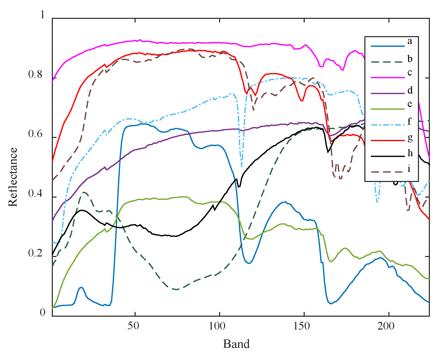
Material optical propertiesDescription of photons’ interactions: bidirectional scattering distribution function (BSDF) model
Ground covers’ spectrum: Tree (a calibrated citrus tree in [70]);
Weed (Lolium sp); Soil (dry Luvisol)
Geometry descriptionsLeaves, branches and trunk are modeled as triangular meshes
Row spacing: 4.5 m; tree spacing: 2 m; tree height: 3 m; row azimuth: 7.3°
Table 12. Comparison of the algorithms for the virtual orchard and real hyperspectral datasets.
DatasetVirtual OrchardAVIRISHYDICE
MSADRMSE S R E L M M (dB)
VCA-FCLS [4,6]7.08740.349428.424323.5525
Fan-NMF [48]7.58510.345923.267320.0746
GBM-semiNMF [38]7.0874 (VCA [4])0.320325.811128.6362
PPNMGDA [32]7.0874 (VCA [4])0.272616.143717.5868
MLM [37]7.0874 (VCA [4])0.276317.969319.6737
DNSPU [46]7.58170.288621.633618.9756
RNMF [54]8.36890.349128.495327.0158
Bio-KNMF [57]7.78680.348029.300030.7360
BCNMF (FM)7.02890.268113.571423.1293
BCNMF (GBM)7.02890.268113.571423.1293
BCNMF (PPNM)6.76190.202717.507119.5446

