Combining TerraSAR-X and Landsat Images for Emergency Response in Urban Environments

Abstract
:
1. Introduction
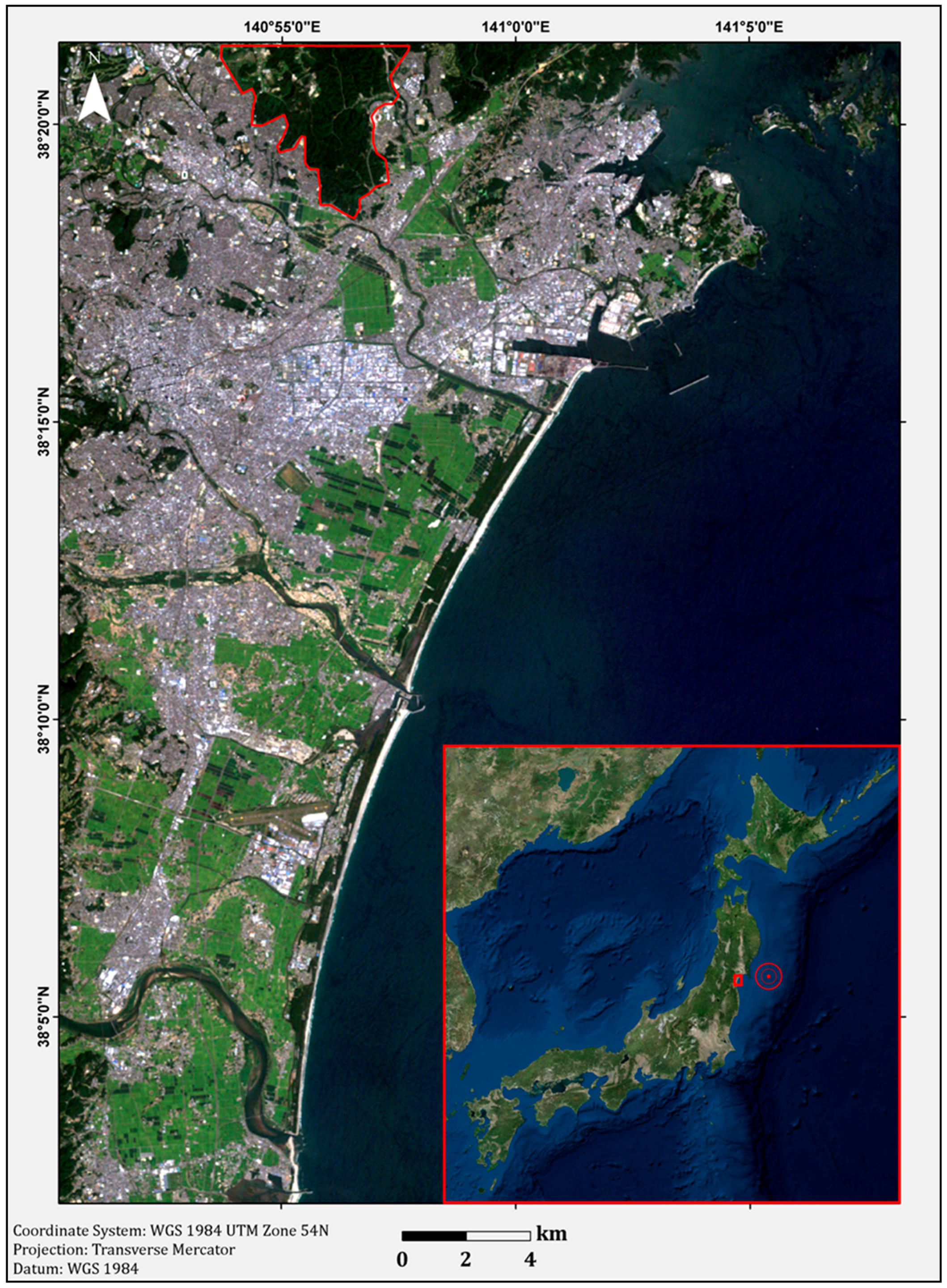
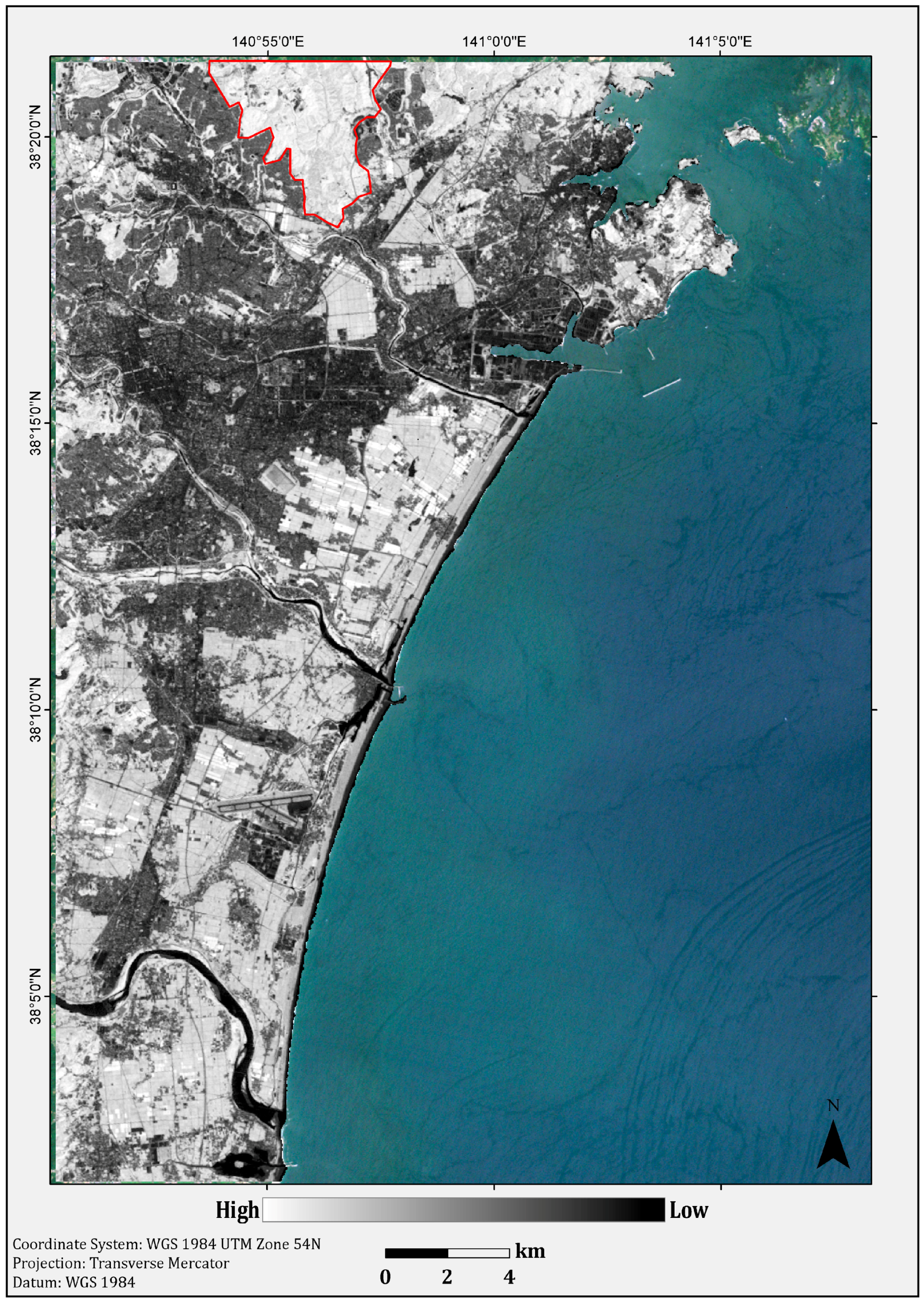
2. Research Area
3. Materials and Methods
3.1. Remote Sensing Data and Pre-Processing
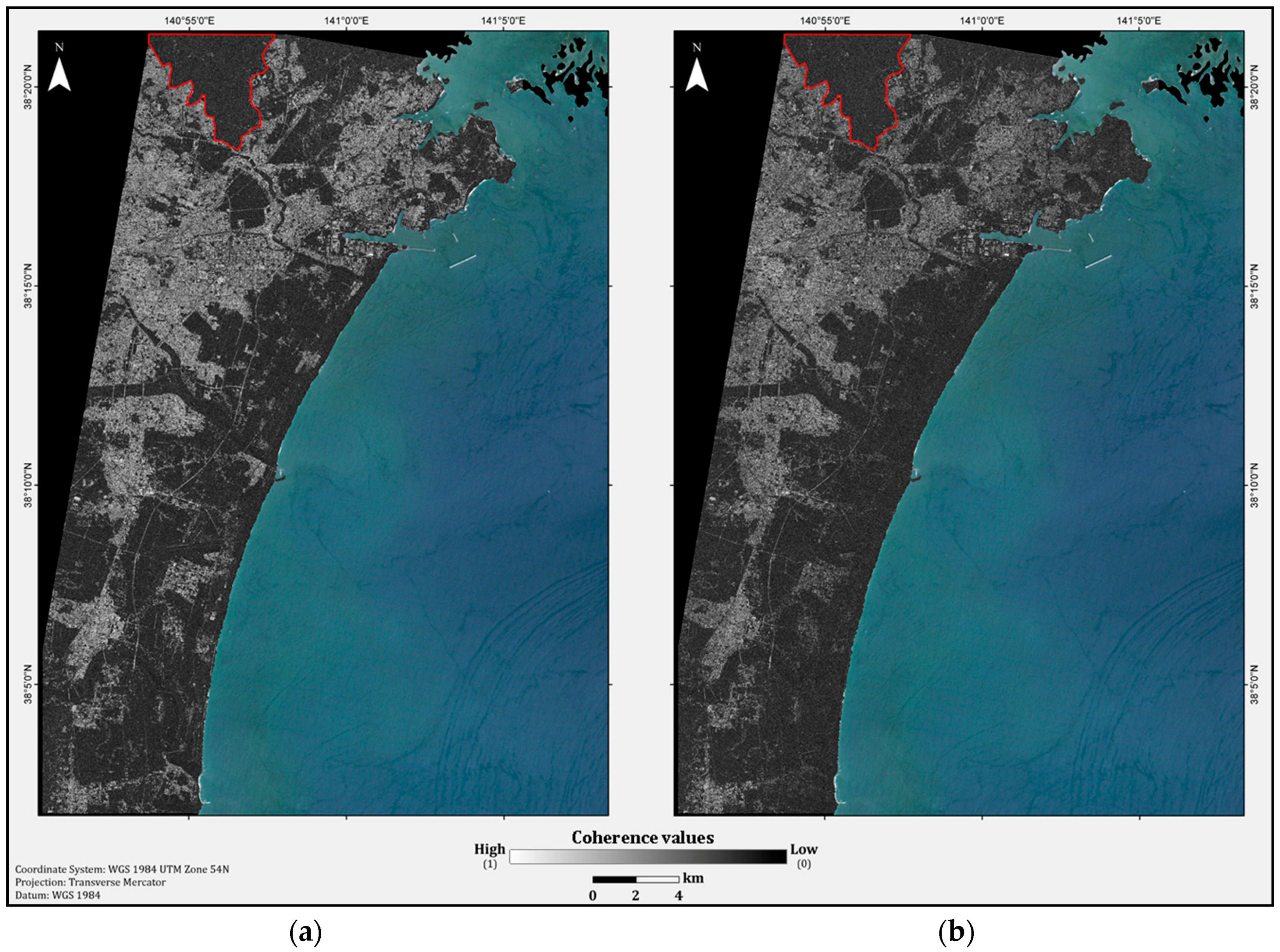
3.2. InSAR Coherence
3.3. Normalized Difference Vegetation Index (NDVI)
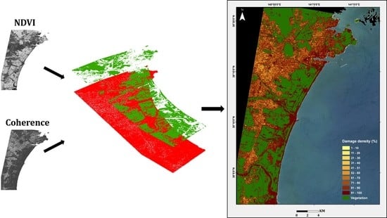
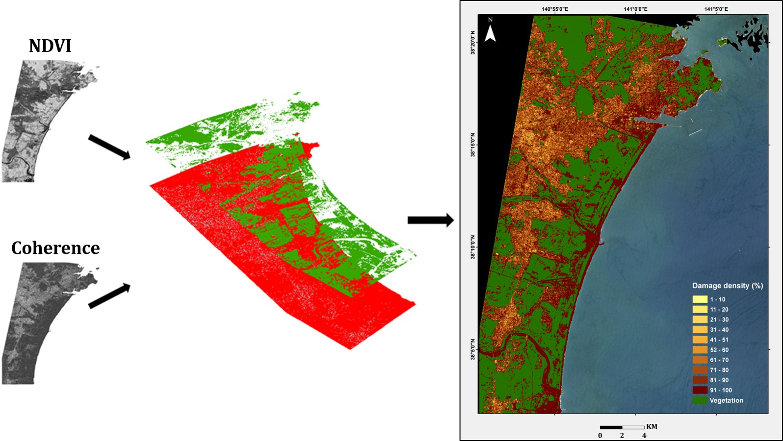
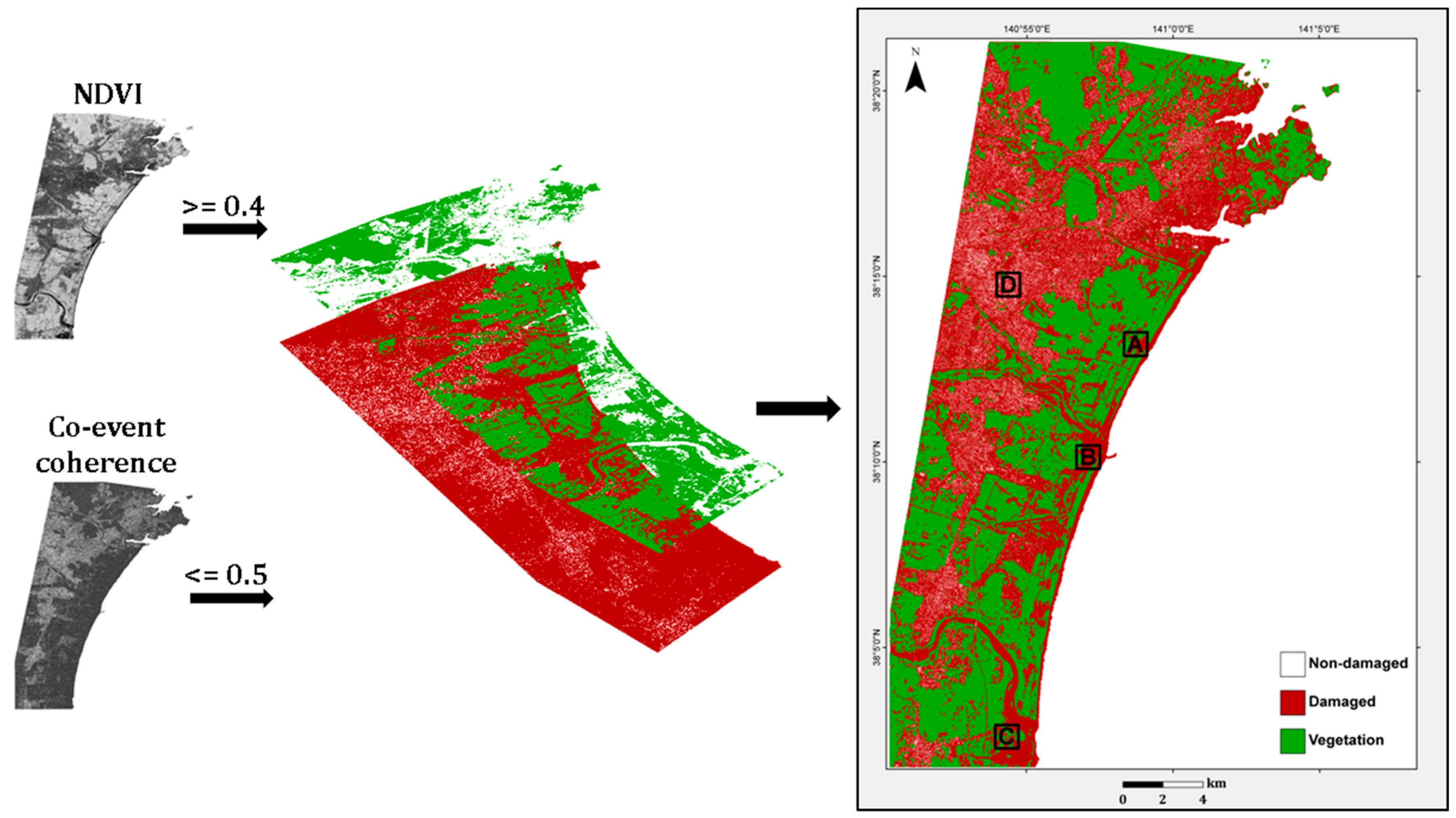
3.4. Combining SAR and Multi-Spectral Data
3.4.1. Setting Thresholds
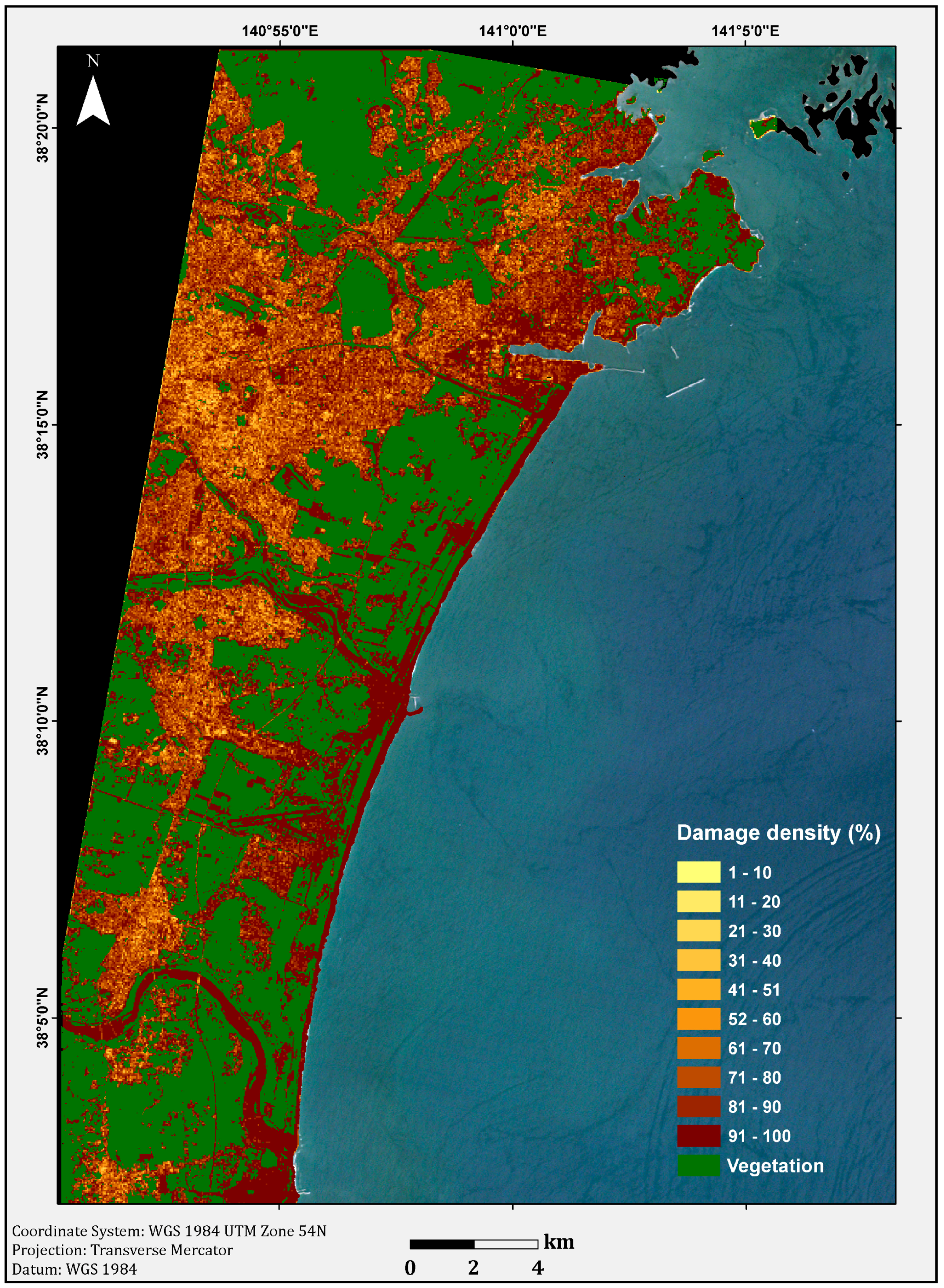
3.4.2. Damage Assessment Map
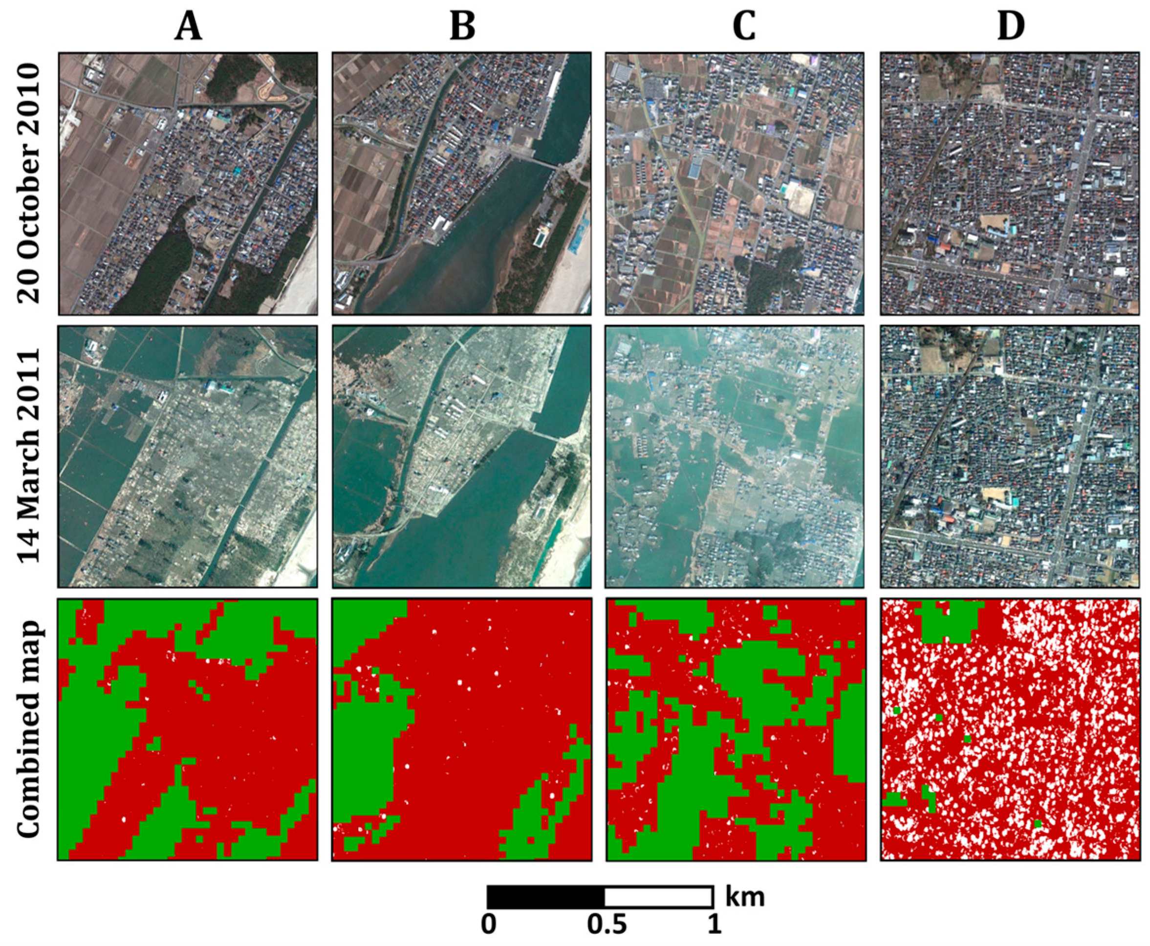
3.5. Accuracy Assessment
4. Results and Discussion
5. Conclusions
Author Contributions
Acknowledgments
Conflicts of Interest
References
- Oštir, K.; Veljanovski, T.; Podobnikar, T.; Stančič, Z. Application of satellite remote sensing in natural hazard management: The Mount Mangart landslide case study. Int. J. Remote Sens. 2003, 24, 3983–4002. [Google Scholar] [CrossRef]
- Plank, S. Rapid damage assessment by means of multi-temporal SAR—A comprehensive review and outlook to Sentinel-1. Remote Sens. 2014, 6, 4870–4906. [Google Scholar] [CrossRef] [Green Version]
- Uprety, P.; Yamazaki, F. Use of high-resolution SAR intensity images for damage detection from the 2010 Haiti earthquake. In Proceedings of the 2012 IEEE International Geoscience and Remote Sensing Symposium (IGARSS), Munich, Germany, 22–27 July 2012; pp. 6829–6832. [Google Scholar]
- Joyce, K.E.; Belliss, S.E.; Samsonov, S.V.; McNeill, S.J.; Glassey, P.J. A review of the status of satellite remote sensing and image processing techniques for mapping natural hazards and disasters. Prog. Phys. Geogr. 2009, 33, 183–207. [Google Scholar] [CrossRef]
- Dong, L.; Shan, J. A comprehensive review of earthquake-induced building damage detection with remote sensing techniques. ISPRS J. Photogramm. Remote Sens. 2013, 84, 85–99. [Google Scholar] [CrossRef]
- Yamazaki, F.; Kouchi, K.; Kohiyama, M.; Muraoka, N.; Matsuoka, M. Earthquake damage detection using high-resolution satellite images. In Proceedings of the 2004 IEEE International Geoscience and Remote Sensing Symposium, IGARSS’04, Anchorage, AK, USA, 20–24 September 2004; pp. 2280–2283. [Google Scholar]
- Saito, K.; Spence, R.J.; Going, C.; Markus, M. Using high-resolution satellite images for post-earthquake building damage assessment: A study following the 26 January 2001 Gujarat earthquake. Earthq. Spectra 2004, 20, 145–169. [Google Scholar] [CrossRef]
- Saito, K.; Spence, R.; de C Foley, T.A. Visual damage assessment using high-resolution satellite images following the 2003 Bam, Iran, earthquake. Earthq. Spectra 2005, 21, 309–318. [Google Scholar] [CrossRef]
- Ferretti, A.; Monti-Guarnieri, A.; Prati, C.; Rocca, F.; Massonet, D. InSAR Principles-Guidelines for SAR Interferometry Processing and Interpretation; ESA Publications: Noordwijk, The Netherlands, 2007. [Google Scholar]
- Chini, M. Earthquake damage mapping techniques using SAR and optical remote sensing satellite data. In Advances in Geoscience and Remote Sensing; InTech: London, UK, 2009. [Google Scholar]
- Hoffmann, J. Mapping damage during the Bam (Iran) earthquake using interferometric coherence. Int. J. Remote Sens. 2007, 28, 1199–1216. [Google Scholar] [CrossRef]
- Fielding, E.J.; Talebian, M.; Rosen, P.A.; Nazari, H.; Jackson, J.A.; Ghorashi, M.; Walker, R. Surface ruptures and building damage of the 2003 Bam, Iran, earthquake mapped by satellite synthetic aperture radar interferometric correlation. J. Geophy. Res. Solid Earth 2005, 110. [Google Scholar] [CrossRef] [Green Version]
- Yamazaki, F. Applications of remote sensing and GIS for damage assessment. In Proceedings of the 8th International Conference on Structural Safety and Reliability, Newport Beach, CA, USA, 17–22 June 2001; pp. 1–12. [Google Scholar]
- Watanabe, M.; Thapa, R.B.; Ohsumi, T.; Fujiwara, H.; Yonezawa, C.; Tomii, N.; Suzuki, S. Detection of damaged urban areas using interferometric SAR coherence change with PALSAR-2. Earth Planets Space 2016, 68, 131. [Google Scholar] [CrossRef]
- Milisavljevic, N.; Closson, D.; Holecz, F.; Collivignarelli, F.; Pasquali, P. An approach for detecting changes related to natural disasters using Synthetic Aperture Radar data. Int. Arch. Photogramm. Remote Sens. Spat. Inform. Sci. 2015, 40, 819–826. [Google Scholar] [CrossRef]
- Romaniello, V.; Piscini, A.; Bignami, C.; Anniballe, R.; Stramondo, S. Earthquake damage mapping by using remotely sensed data: The Haiti case study. J. Appl. Remote Sens. 2017, 11, 016042. [Google Scholar] [CrossRef]
- Matsuoka, M.; Yamazaki, F. Use of satellite SAR intensity imagery for detecting building areas damaged due to earthquakes. Earthq. Spectra 2004, 20, 975–994. [Google Scholar] [CrossRef]
- Yonezawa, C.; Takeuchi, S. Decorrelation of SAR data by urban damages caused by the 1995 Hyogoken-nanbu earthquake. Int. J. Remote Sens. 2001, 22, 1585–1600. [Google Scholar] [CrossRef]
- Arciniegas, G.A.; Bijker, W.; Kerle, N.; Tolpekin, V.A. Coherence-and amplitude-based analysis of seismogenic damage in Bam, Iran, using Envisat ASAR data. IEEE Trans. Geosci. Remote Sens. 2007, 45, 1571–1581. [Google Scholar] [CrossRef]
- Liao, M.; Jiang, L.; Lin, H.; Huang, B.; Gong, J. Urban change detection based on coherence and intensity characteristics of SAR imagery. Photogramm. Eng. Remote Sens. 2008, 74, 999–1006. [Google Scholar] [CrossRef]
- Dell’Acqua, F.; Gamba, P. Remote sensing and earthquake damage assessment: Experiences, limits, and perspectives. Proc. IEEE 2012, 100, 2876–2890. [Google Scholar] [CrossRef]
- Preiss, M.; Stacy, N.J. Coherent change detection: Theoretical description and experimental results. J. Am. Dent. Assoc. 2006, 38, 365–372. [Google Scholar]
- Tamkuan, N.; Nagai, M. Fusion of multi-temporal interferometric coherence and optical image data for the 2016 kumamoto earthquake damage assessment. ISPRS Int. J. Geo-Inf. 2017, 6, 188. [Google Scholar] [CrossRef]
- Mori, N.; Takahashi, T.; Yasuda, T.; Yanagisawa, H. Survey of 2011 Tohoku earthquake tsunami inundation and run-up. Geophys. Res. Lett. 2011, 38. [Google Scholar] [CrossRef]
- Kazama, M.; Noda, T. Damage statistics (Summary of the 2011 off the Pacific Coast of Tohoku Earthquake damage). Soils Found. 2012, 52, 780–792. [Google Scholar] [CrossRef]
- Hanssen, F.R. RADAR Interferometry: Data Interpretation and Error Analysis, 1st ed.; Springer: Dordrecht, The Netherlands, 2002. [Google Scholar]
- Havivi, S.; Amir, D.; Schvartzman, I.; August, Y.; Maman, S.; Rotman, S.R.; Blumberg, D.G. Mapping dune dynamics by InSAR coherence. Earth Surf. Process Landf. 2017, 43, 1229–1240. [Google Scholar] [CrossRef]
- Zebker, H.A.; Villasenor, J. Decorrelation in interferometric radar echoes. IEEE Trans. Geosci. Remote Sens. 1992, 30, 950–959. [Google Scholar] [CrossRef]
- Rosen, P.A.; Hensley, S.; Joughin, I.R.; Li, F.K.; Madsen, S.N.; Rodriguez, E.; Goldstein, R.M. Synthetic aperture radar interferometry. Proc. IEEE 2000, 88, 333–382. [Google Scholar] [CrossRef]
- Hong, S.; Wdowinski, S.; Kim, S. Evaluation of TerraSAR-X observations for wetland InSAR application. IEEE Trans. Geosci. Remote Sens. 2010, 48, 864–873. [Google Scholar] [CrossRef]


| Satellite | Sensor Type | Acquisition Date | Resolution | Spectral Properties | |
|---|---|---|---|---|---|
| TerraSAR-X | SAR | Pre-event | 21 September 2008 | 2 m | SLC |
| Pre-event | 20 October 2010 | X-band | |||
| Post-event | 12 March 2011 | HH polarization | |||
| Landsat5 TM | Multispectral | Pre-event | 24 August 2010 | 30 m | 7 bands |
| Entire Scene | A | B | C | D | |||||||
|---|---|---|---|---|---|---|---|---|---|---|---|
| PA | UA | PA | UA | PA | UA | PA | UA | PA | UA | ||
| 50 m | Vegetation | 89 | 97 | 90 | 100 | 92 | 85 | 96 | 88 | 50 | 100 |
| Damage | 96 | 76 | 100 | 90 | 95 | 97 | 88 | 88 | 100 | 80 | |
| No/slight damage | 87 | 92 | 50 | 100 | 0 | 0 | 0 | 0 | 95 | 95 | |
| Overall accuracy | 89 | 94 | 94 | 88 | 92 | ||||||
| Kappa coefficient | 82 | 88 | 84 | 77 | 79 | ||||||
| 100 m | Overall accuracy | 82 | |||||||||
| Kappa coefficient | 68 | ||||||||||
© 2018 by the authors. Licensee MDPI, Basel, Switzerland. This article is an open access article distributed under the terms and conditions of the Creative Commons Attribution (CC BY) license (http://creativecommons.org/licenses/by/4.0/).
Share and Cite
Havivi, S.; Schvartzman, I.; Maman, S.; Rotman, S.R.; Blumberg, D.G. Combining TerraSAR-X and Landsat Images for Emergency Response in Urban Environments. Remote Sens. 2018, 10, 802. https://doi.org/10.3390/rs10050802
Havivi S, Schvartzman I, Maman S, Rotman SR, Blumberg DG. Combining TerraSAR-X and Landsat Images for Emergency Response in Urban Environments. Remote Sensing. 2018; 10(5):802. https://doi.org/10.3390/rs10050802
Chicago/Turabian StyleHavivi, Shiran, Ilan Schvartzman, Shimrit Maman, Stanley R. Rotman, and Dan G. Blumberg. 2018. "Combining TerraSAR-X and Landsat Images for Emergency Response in Urban Environments" Remote Sensing 10, no. 5: 802. https://doi.org/10.3390/rs10050802