Long-Term Validation of TerraSAR-X and TanDEM-X Orbit Solutions with Laser and Radar Measurements

Abstract

Precise orbit determination solutions for the two spacecrafts TerraSAR-X (TSX) and TanDEM-X (TDX) are operationally computed at the German Space Operations Center (GSOC/DLR). This publication makes use of 6 years of TSX and TDX orbit solutions for a detailed orbit validation. The validation compares the standard orbit products with newly determined enhanced orbit solutions, which additionally consider GPS ambiguity fixing and utilize a macro model for modeling non-gravitational forces. The technique of satellite laser ranging (SLR) serves as a key measure for validating the derived orbit solutions. In addition, the synthetic aperture radar (SAR) instruments on-board both spacecrafts are for the first time employed for orbit validation. Both the microwave instrument and the optical laser approach are compared and assessed. The average SLR residuals, obtained from the TSX and TDX enhanced orbit solutions within the analysis period, are at $1.6\pm 11.4$ mm ($1\sigma$) and $1.2\pm 12.5$ mm, respectively. Compared to the standard orbit products, this is an improvement of 33 % in standard deviation. The corresponding radar range biases are in the same order and amount to $-3.5\pm 12.5$ mm and $4.5\pm 14.9$ mm. Along with the millimeter level position offsets in radial, along-track and cross-track inferred from the SLR data on a monthly basis, the results confirm the advantage of the enhanced orbit solutions over the standard orbit products.

1. Introduction

The TerraSAR-X satellite mission [1,2] consists of the two spacecrafts: TSX and TDX, which are equipped with Synthetic Aperture Radar (SAR) instruments for active remote sensing. The ongoing mission is successfully observing the Earth for more than 10 years. Precise information on the satellite positions is of vital importance for many of its SAR applications, e.g., for SAR imaging geodesy [3,4,5,6] or the generation of the global digital elevation model from bistatic interferometry [7]. The satellite orbits are determined by the German Space Operations Center (GSOC) in a reduced-dynamic approach, which incorporates measurements from the onboard Global Positioning System (GPS) receivers as well as the modeling of gravitational and non-gravitational forces [8]. For orbit validation, the technique of Satellite Laser Ranging (SLR) is widely used and embedded as state-of-the-art [9,10]. Data obtained from various laser ranging stations for TSX and TDX, and the notably high ranking of the mission in the tracking priority list provide highly reliable SLR data. In addition to the laser reflector, the spacecrafts are equipped with accurate SAR instruments as primary payloads. The SAR enables ranging measurements from the spacecrafts to on-ground trihedral Corner Reflector (CRs), which provide a sharp reflection of the transmitted chirp signals, and thus can also provide high accuracy in ranging if the data is processed according to geodetic standards [5,6,11]. Therefore, the orbit analysis published in this paper makes use of both SLR and SAR measurements. The derived SAR and SLR measurements are compared in terms of residuals, and estimated spacecraft position offsets. SLR allows estimation of the offsets in radial, along-, and cross-track direction, which is comparable to the range and azimuth residuals, obtained from the SAR analysis.

The remainder of the publication is structured as follows. Section 2 and Section 3 describe the TerraSAR-X orbit, the payloads and methods used for precise orbit determination, as well as the orbit solutions investigated in our study. Section 4 provides the details on the SLR and the SAR ranging techniques, including descriptions of the data sets and the contributing geodetic stations. In Section 5, we present and discuss the results for each of the two techniques, and provide a comparative analysis based on monthly estimates for the remaining offsets. The paper concludes with Section 6 with a discussion of the key findings and the final conclusions.

2. Spacecrafts and Orbits

For the present study, two different satellite orbit solutions of the spacecrafts TSX and TDX are analyzed. The spacecrafts were launched on 15 June 2007, and 21 June 2010, respectively [2,12], which enables us to study the long-term behavior of the orbit solutions. The aim of the TerraSAR-X mission is Earth observation, based on individual, or combined SAR observations of the Earth surface. The GSOC at the German Aerospace Center (DLR) in Oberpfaffenhofen, Germany, is in charge of mission control and the operational orbit determination. Both spacecrafts are orbiting the Earth on a Sun-synchronous, 97.44° inclined dusk-dawn orbit at an average altitude of 514 km. The orbital period is roughly 90 minutes, and one complete orbital repeat cycle takes 11 days, which provides high repeatability [13,14]. Due to the chosen orbit configuration along with the terminator, the spacecraft is almost constantly illuminated by the Sun. Due to the objective of the interferometric campaigns, the strict orbit requirements for TerraSAR-X are formulated in the form of a 250 m toroidal tube around a pre-flight determined reference trajectory. Star trackers for attitude determination, reaction wheels and magnetorquers for momentum unloading are utilized for determining the spacecrafts attitude with a pointing accuracy smaller than 40 arcsec [12].

The spacecrafts are equipped with identical payloads, of which the SAR payload primarily serving the Earth observation is employed for additional orbit validation within this study. An illustration of the spacecraft TerraSAR-X is shown in Figure 1, indicating the SAR and SLR payloads.

For the purpose of attitude and orbit determination, each spacecraft is equipped with star trackers for attitude determination, as well as three GPS receivers. The Integrated Geodetic and Occultation Receiver (IGOR) serves as the primary receiver for Precise Orbit Determination (POD) and baseline reconstruction, and provides geodetic-grade dual-frequency measurements [15]. The second and third are MosaicGNSS receivers, which mainly serve for on-board timing and basic orbit information for aligning the spacecraft with the ground track and the nadir direction [16]. In addition, both spacecrafts carry a Laser Retro Reflector (LRR), which allows accurate orbit validation with SLR. The IGOR receiver and the LRR unit are contributed by the University of Texas Center for Space Research and the Deutsches GeoForschungsZentrum Potsdam (GFZ).

3. Precise Orbit Determination Concept and Models

Precise orbit determination solutions of TSX and TDX are computed at GSOC, applying the method of reduced-dynamic orbit determination. DLR’s GNSS High Precision Orbit Determination Software Tools (GHOST) are utilized for POD and SLR validation [17]. The orbit determination employs a dynamical orbit model considering gravitational and non-gravitational forces, as well as complementary empirical accelerations, which are modeled in addition to the initial daily state vector of the satellite and the scaling factors for individual force model constituents. Estimation parameters with respect to the on-board GPS measurements include the epoch-wise receiver clock offsets and an integer-valued ambiguity of the ionosphere-free carrier phase combination for each continuous tracking pass.

Non-gravitational accelerations for Earth and solar radiation pressure, as well as the aerodynamic accelerations, are considered by a macro model formulation, which approximates the spacecraft as an extruded, equilateral hexagon [18].

GPS observations from the geodetic-grade IGOR receiver are considered by ${\mathrm{L}}_1$ and ${\mathrm{L}}_2$ code and phase measurements, which are combined in a ionosphere-free linear combination. In addition, a single-receiver ambiguity resolution concept is employed that builds on dedicated GPS orbit, clock, and wide-lane bias products provided by the CNES/CLS (Centre National d’Études Spatiales/Collecte Localisation Satellites) analysis center of the International GNSS Service (IGS) [19].

Table 1. GHOST models and data sets for TerraSAR-X precise orbit determination.

GPS Measurement
GPS observations	Undifferenced ${\mathrm{L}}_1$/${\mathrm{L}}_2$ pseudorange and carrier phase range, 30-s sampling, daily arcs
GPS orbits and clocks	CNES-CLS grg products [20], 30-s sampling
GPS satellite antenna	IGS igs08.atx/igs14.atx phase center offsets and variation [21]
GPS satellite biases	CNES-CLS wide-lane satellite biases [20], ftp://ftpsedr.cls.fr/pub/igsac/
GPS antenna	PCO + PV corrections from in-flight calibration; center-of-mass variation
Attitude	Quaternions (measured)
Reference frame	IGb08 [21], IGS14 [22], from DOY 30/2017 onwards
Phase windup	Modeled [23]
Orbit
Earth gravity field	GOCO03S [24] up to order and degree 100; rate terms ${\dot{C}}_{20}$, ${\dot{C}}_{21}$, ${\dot{S}}_{20}$
Luni-solar gravity	Point-mass model; analytical series of luni-solar coordinates
Solid Earth and pole tides	IERS2003
Ocean tides	CSR/Topex3.0 [25]
Relativity	Post-Newtonian correction
Spacecraft parameters	Time-varying mass (≈1319 kg); 8 panel box-wing macro-model
Solar radiation pressure	Macro-model; conical Earth shadow model
Earth radiation pressure	Macro-model; CERES Earth radiation data [26]
Aerodynamics	Macro-model; NRLMSISE-00 density model [27], NOAA/SWPC solar flux and geomagnetic activity data (ftp://tp.swpc.noaa.gov/pub/indices/)
Maneuvers	Constant thrust in RTN direction
Empirical acceleration	Piecewise constant accelerations in RTN direction; 10-min intervals
Reference frame	ICRF
Earth orientation	IERS1996; IGS final EOPs; center-of-mass/center-of-figure offset
Numerical integration	Self-starting variable-order variable step size multistep method [28]
Estimation
Filter	Batch least squares estimation
Estimation parameters	Epoch state vector, scale factors for SRP and drag/lift, empirical accelerations and maneuvers, clock offsets, phase ambiguities
Stochastic models	White observation noise, elevation-independent

shows an overview of the employed key models and parameters that have been used to generate the enhanced orbit solutions, which are the main scope of the present study. These orbit solutions are abbreviated and referred to in the following as ENHanced (ENH). Note that the orbit solution described above is not identical to the operationally computed Precise Science Orbit (PSOs), which consider non-gravitational forces combined with a simplified satellite shape (cannon-ball model), and employ float GPS ambiguities [18]. The PSOs are utilized for ease of comparison only. Regarding the temporal coverage, this analysis covers both orbit solutions for TSX and TDX during the period of 1 January 2012 to 31 December 2017.

4. Orbit Validation Techniques

In the field of precise orbit determination, SLR is well-established as a state-of-the-art validation technique, since it provides independent measurements of high quality and reliability [10]. Additionally, we present a long-term analysis of SAR range and azimuth residuals derived from the measurements of the TerraSAR-X radar payloads, which for the first time provide a second independent method to validate the impact of the enhanced orbit solution. Both methods rely on global geodetic ground infrastructure, which is visualized in Figure 2. On the SLR side, the measurements are obtained by 11 International Laser Ranging Service (ILRS) [29] stations, while the SAR measurements are supported by five CRs located at three stations. The following sections discuss both methods, and provide further details on the data reduction and the processing strategies.

4.1. Satellite Laser Ranging

4.1.1. Technique

Satellite laser ranging observations are optical two-way runtime measurements from ground stations to the LRR on-board the satellite. The LRR of TSX and TDX comprises four individual prisms in a rotationally symmetric arrangement [30], see Figure 3, to ensure reliable reflection properties over a wide range of incidence angles. The individual prisms are arranged in a regular $45°$ pyramid.

Basically, the ground station actively emits a laser pulse, which is reflected by the prisms on the spacecraft. The runtime measurements translate into the range $r_{\mathrm{SLR}}$, which is compared to the geometric range derived from the orbit solutions $r_{\mathrm{POD}}$:

$$\Delta r=r_{\mathrm{SLR}}-r_{\mathrm{POD}}.$$

(1)

The obtained SLR range residuals $\Delta r$ are a measure of the orbit accuracy. Of vital importance are the well-known positions of the LRR onboard the spacecraft and of the laser tracking stations on ground. The coordinates of the LRR were precisely determined along with the phase patterns of the optical systems during the pre-flight calibration on ground, see

Table 2. Selected models for Satellite Laser Ranging orbit validation.

Station coordinates	SLRF2014 [31]
Solid Earth and pole tides	IERS2003
Ocean tide loading	GOT00.2 [32]
Tropospheric refraction	IERS2010 [33]
Relativity	Space-time curvature correction
LRR phase correction	Neubert et al. [30]

. The SLR station coordinates, on the other hand, are related to the terrestrial frame and its models are discussed in the next section.

Satellite laser ranging residuals, which are obtained from the approach as described above, do not contain any information on the 3-D spatial variation of the residuals across individual tracking passes. Therefore, an extended validation approach has been published in Hackel et al. [18], where the obtained SLR residuals are further utilized for estimating SLR-based position offsets of the spacecraft. The extended data interval of 30 days serves as the basis for monthly position estimates in the spacecraft’s radial, along-track, and cross-track direction.

4.1.2. Models

The modeling of SLR makes use of station coordinates, which refer to the Satellite Laser Ranging Frame 2014 (SLRF2014) [31]. This ensures best consistency with the IGb08, and IGS14 frames of the GPS orbit products, which are employed in the orbit determination of the TSX and TDX orbit solutions [22,34]. The phase center range correction of the LRR of each spacecraft is considered as a function of azimuth with respect to local spacecraft heading and the nadir angle, and is provided by the GFZ [30]. The selected models for solid Earth tides, ocean tidal loading, and tropospheric refraction are introduced in Table 2.

4.1.3. Tracking Data Analysis

The SLR tracking data are provided by the ILRS, which observes a multitude of satellites according to a mission priority list. The spacecrafts TSX and TDX are highly ranked at positions 3 and 2 [35], which results in a large number of tracking points. The SLR measurements are averaged in time intervals of 5 s, which finally result in one Normal Point (NP) [36]. The number of normal points within one tracking pass, i.e., the passage where the instrument on ground follows and tracks the spacecraft may vary from pass to pass. For TSX, on average 15 NPs are collected during one tracking pass, which corresponds to an average tracking length of 75 s.

Within the six year period, the spacecraft TSX was tracked by 34 different ILRS stations, yielding a wide range from only 5 to up to $75,000$ normal points per station. For the present study, a subset of 11 reliable and high-performance ILRS stations has been selected, which are shown in Figure 2.

Considering the 11 stations, a total of $206,401$ normal points is available for TSX within the 6 years (cf. Figure 4). Applying an elevation cutoff-angle of $10°$, and a threshold of 6 cm for the residuals, this leads to a total of $204,667$ NPs, which are employed within this study. This corresponds to a screening rate of $0.84\%$. For the spacecraft TDX, the number of accepted normal points used throughout this analysis amounts to $195,506$. Despite the higher ranking of TDX, the number of available normal points during the analysis period is slightly larger for TSX.

4.2. Radar Ranging

4.2.1. Technique

Similar to SLR, a spaceborne SAR payload allows for the measurement of the 2-way signal round trip time between the sensor and the ground. Contrary to the transmission and reception of laser pulses dedicated to the pass of an individual satellite, the radar instrument illuminates a large footprint in side-looking geometry and discriminates the echoes according to the time of flight and the time of reception [37]. Provided that the SAR image processor employs strict geometrical standards, the processing of this raw data matrix for the actual SAR image is able to accurately preserve this underlying timing information. In particular, the often used approximations that reduce computational efforts need to be avoided, for instance the simplification of the platform movement during signal transmission and signal reception, which is also known as ’stop-go’ approximation [37].

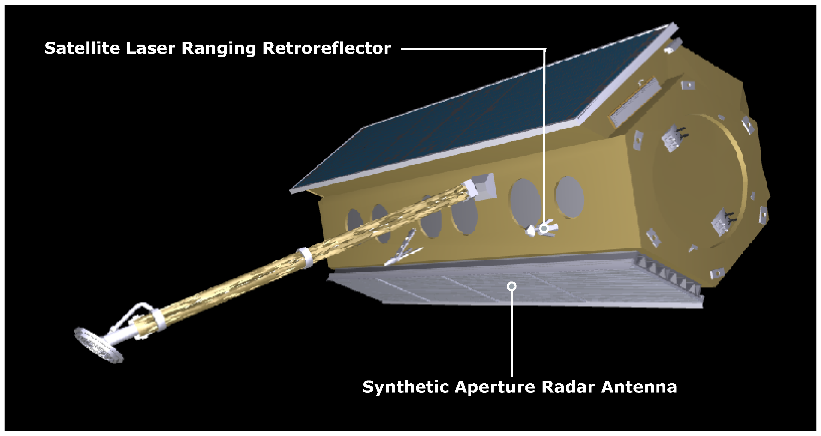
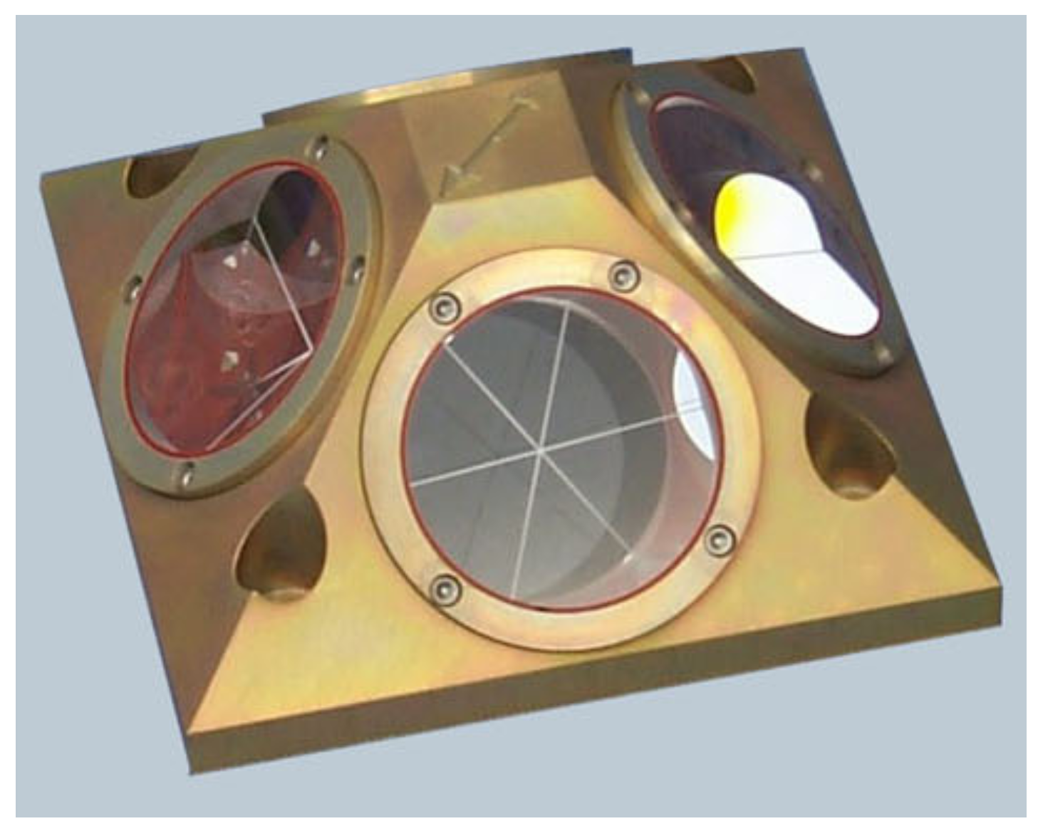
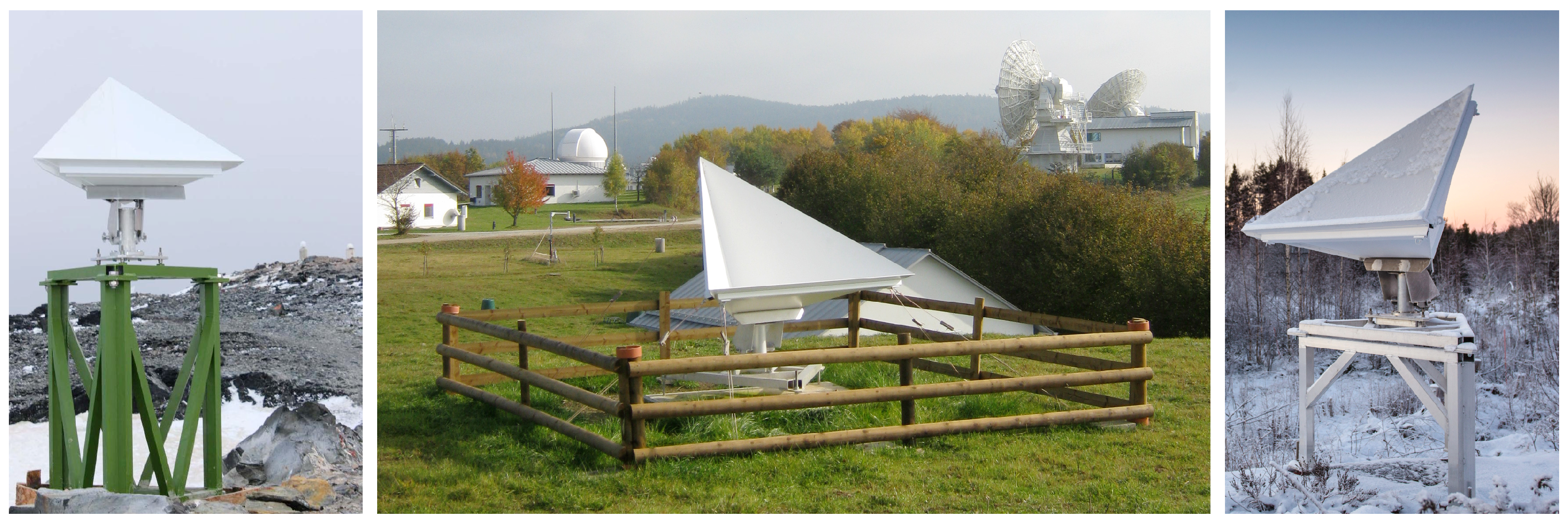
For the TerraSAR-X mission, all these SAR-related aspects have been carefully resolved in the TerraSAR-X Multimode SAR Processor (TMSP). The processor generates well-defined level 1b radar images with each pixel referring to the time of closest approach (zero-Doppler time) and the corresponding two-way round trip time [38,39]. In order to accurately relate this 2-D timing information to a dedicated location within the image, one may create a bright point response by placing a trihedral CR, see Figure 5. From the SAR sensor perspective, the CR needs to be large enough to offer a strong signal return in the radar image, and it must fulfill tight limits in terms of plate orthogonality, planar surface geometries, and mechanical stability [40]. If such a reflector is permanently installed and the reference coordinates are known in the International Terrestrial Reference Frame (ITRF, for the latest release 2014 see [22]), then the SAR measurements may be verified on a pass by pass basis by analyzing the radar timings. As already discussed for the SLR, the terrestrial CR coordinates have to be consistent with IGb08 and IGS14 frame realizations used in the orbit determination.

In accordance with the TerraSAR-X imaging model, we use the range-Doppler equations [37] in zero-Doppler geometry, which relate the satellite trajectory, given by the time-dependent position vector ${\mathbf{X}}_s$ and velocity vector ${\dot{\mathbf{X}}}_s$, and the reflector position vector ${\mathbf{X}}_r$ with the observed radar times t and $\tau$, also referred to as slow time and fast time or azimuth and range, respectively.

$$\begin{array}{cc}\hfill \tau & =2/c·\left|{\mathbf{X}}_s\left(t\right)-{\mathbf{X}}_r\right|\hfill \end{array}$$

(2)

$$\begin{array}{cc}\hfill 0& =\frac{{\dot{\mathbf{X}}}_s\left(t\right)·\left({\mathbf{X}}_s\left(t\right)-{\mathbf{X}}_r\right)}{\left|{\dot{\mathbf{X}}}_s\left(t\right)\right|·\left|{\mathbf{X}}_s\left(t\right)-{\mathbf{X}}_r\right|}\hfill \end{array}$$

(3)

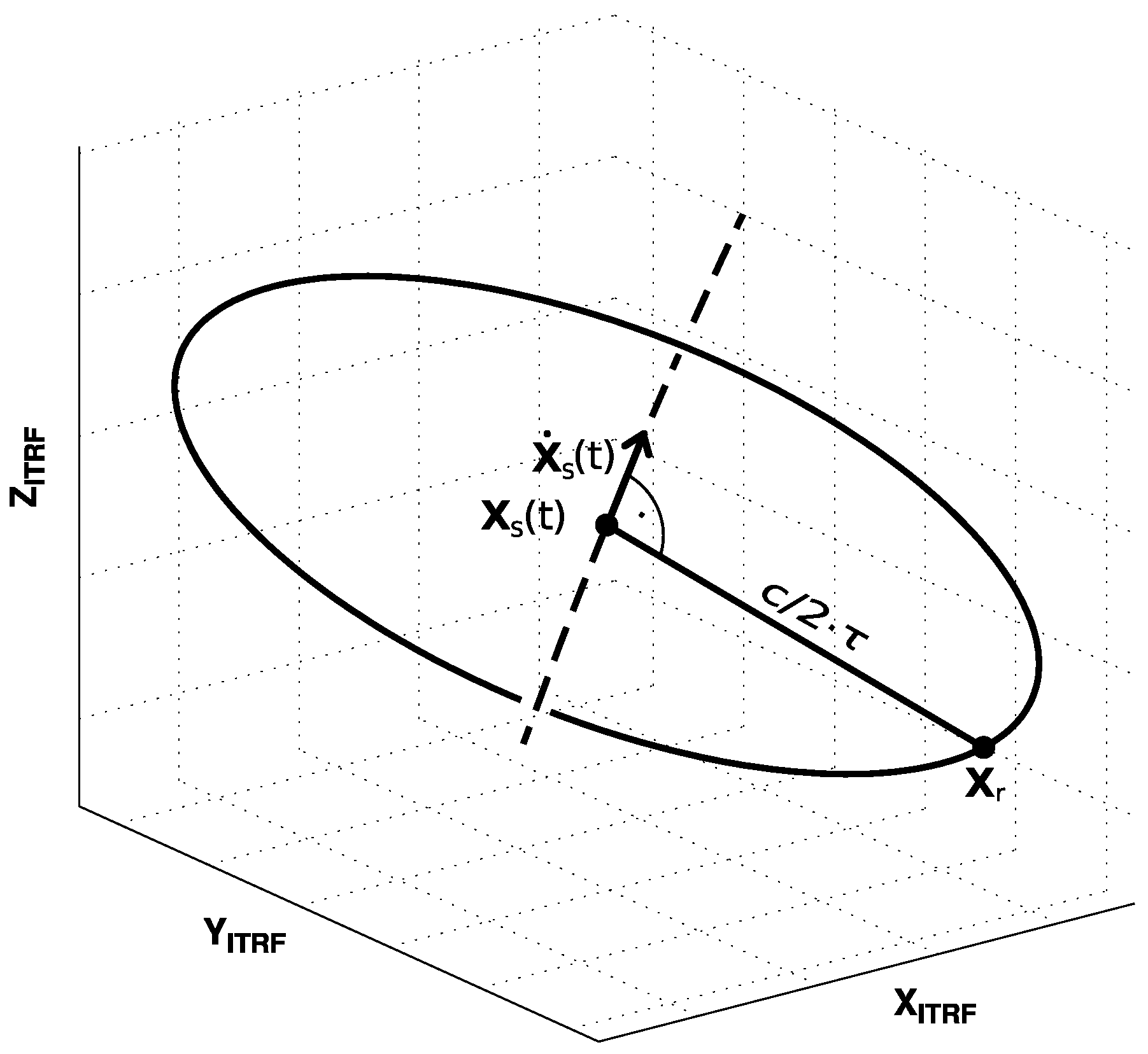
The conversion of geometrical distance for the $\tau$ uses the speed of light in vacuum c. The slow time t is linked to the satellite trajectory and can be resolved by interpolating a given orbit solution and performing an iterative search for the instant of Doppler-zero using the Equation (3). Subsequently, the corresponding round trip time $\tau$ is derived from Equation (2). From a geometrical point of view, the combination of the Equations (2) and (3) models a circle located at the satellite’s zero-Doppler position and oriented according to the zero-Doppler plane, and which intersects with the reflector position on ground, see Figure 6.

In order to compute the reference radar times from the geometric model, the tidal-related solid Earth effects have to be taken into account when defining the ${\mathbf{X}}_r$ for each pass. This is identical to the modeling of SLR station coordinates or other reference markers in the ITRF, see Section 4.1.2 and Table 2. The details of the ITRF models that have to be applied are given in the conventions issued by the International Earth Rotation and Reference Systems Service (IERS) [41]. We include all the models listed in chapter 7 of the conventions in our SAR analysis, and the reflector position ${\mathbf{X}}_r$ is corrected for the epoch of the image acquisition before computing the reference timings with the Equations (2) and (3).

The measured radar timings are extracted from the images by performing the so-called point target analysis [11], which detects the center of the reflector’s point signature in the image with better than $1/1000$ of a pixel. The precision of the extraction in range and azimuth is equivalent to the signal-to-noise ratio, or Signal to Clutter Ratio (SCR) in radar terminology, and may be expressed by [42,43]:

$${\sigma }_{R,A}=\frac{\sqrt{3}}{\pi \sqrt{2}}·\frac{{\rho }_{R,A}}{\sqrt{\mathrm{SCR}}}$$

(4)

The ${\rho }_{R,A}$ denotes the image resolution in range and azimuth, respectively. For the CRs with 0.7 m and 1.5 m inner leg dimension that we use in our study, see Section 4.2.2, we determined a typical SCR of 31 dB and 46 dB for the TerraSAR-X high resolution spotlight images (0.6 m by 1.1 m resolution, [39]) employed in the analysis. According to Equation (4), these SCR values translate into range and azimuth precisions at the millimeter to centimeter level, see

Table 3. Expected range and azimuth localization precision computed from Equation (4) for the TerraSAR-X high resolution spotlight mode and the reflectors used in our study.

CR Inner Leg	SCR [dB]	${\mathit{\sigma }}_{\mathit{R}}$ [mm]	${\mathit{\sigma }}_{\mathit{A}}$ [mm]
0.7 m	31	$6.6$	$12.1$
1.5 m	46	$1.2$	$2.1$

.

Regarding the TerraSAR-X azimuth measurements, a limitation was found in the link between the GPS time provided by the secondary MosaicGNSS receiver (cf. Section 2) and the SAR payload, but this could be improved to about 1–2 cm by exploiting the accurately known pulse repetition interval of the SAR instrument [44]. For the range measurements, additional corrections are required for the atmospheric path delays, for which we rely on the permanently operated GNSS receivers at the geodetic stations hosting the CRs. The slant range tropospheric delay is computed from the zenith delay product provided on a daily basis by the IGS [45], and the slant range ionospheric delay is inferred from the dual-frequency GNSS observations at the stations. The details of our methods are given in [5]. The tropospheric products are estimated with an accuracy of better than 5 mm [45], whereas the cross-comparison of the ionospheric delays from the two or more GNSS receivers available at each of our test sites indicate a similar 5 mm quality level for the ionospheric correction. Finally, there are the range and azimuth geometrical calibration constants of the SAR instrument, which need to be determined in dedicated experiments, as described in Section 4.2.3.

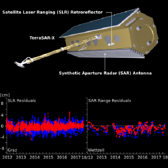
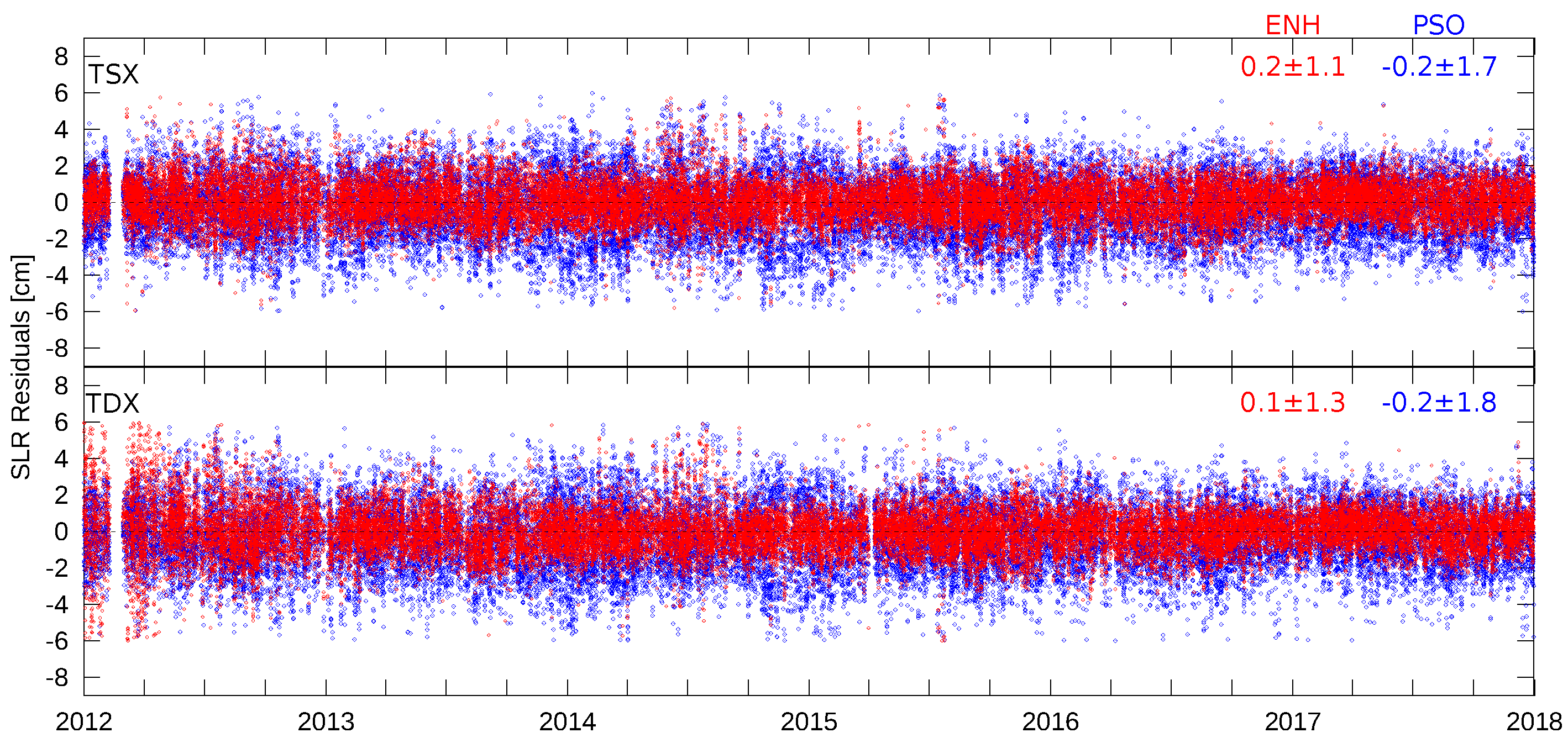
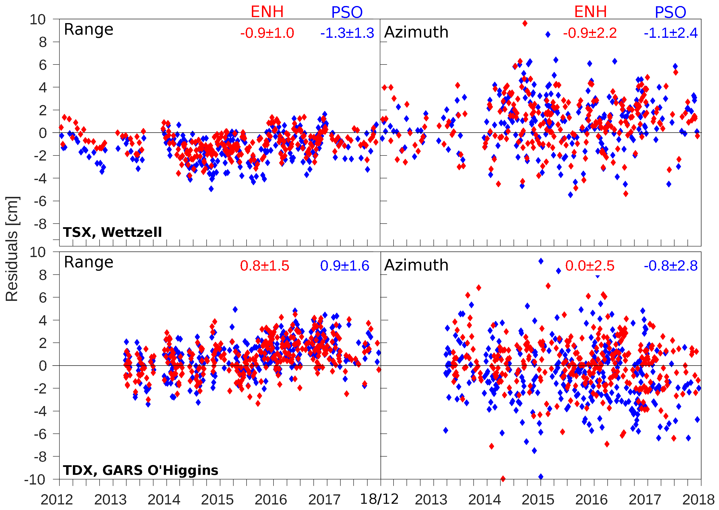
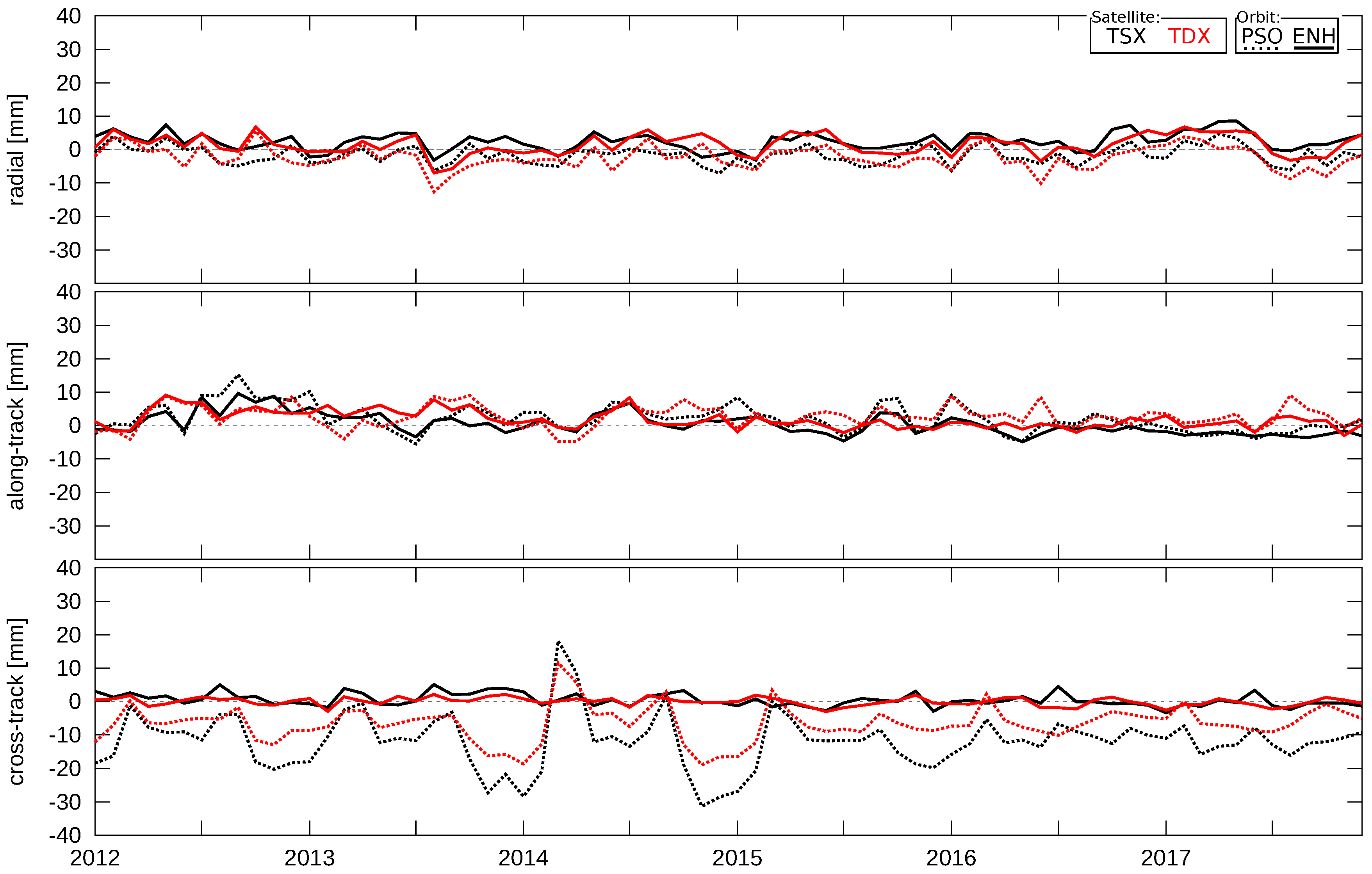
In summary, the combination of CRs with reference coordinates and the orbit solution allows for the computation of residuals in range and azimuth using the radar payload. The correction of the atmospheric path delay in the measurements and the modeling of the reference coordinates according to the geodetic conventions ensure accurate SAR-based residuals, which are also useful when testing different orbit solutions. Like in the case of SLR, the SAR residuals may be interpreted as orbital errors and can in principle be decomposed into radial, along-track and cross-track residuals [18]. However, it has to be emphasized that the SAR provides only one range per pass, i.e., the range at the instant of zero-Doppler, and the corresponding azimuth is basically the along-track error, whereas the SLR enables the tracking of the entire pass.

4.2.2. Ground Infrastructure

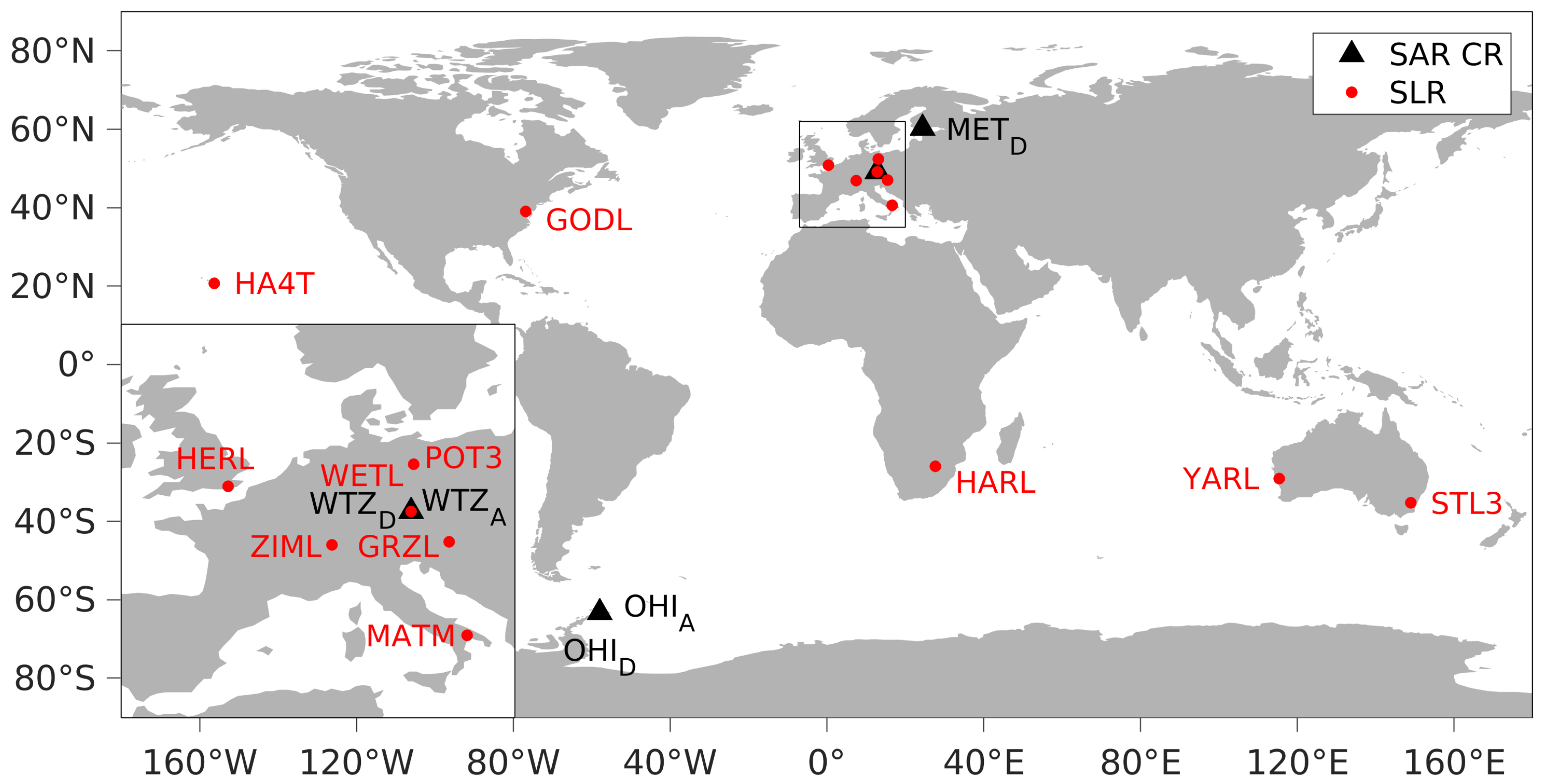
In the course of our long-term monitoring of the geometrical quality of TerraSAR-X, the three geodetic stations marked in Figure 2 have become equipped with permanent CR installations, see Figure 5. The Wettzell geodetic station in Germany hosts two CRs with 1.5 m inner leg dimension, with one CR aligned for the ascending passes (${\mathrm{WTZ}}_A$) and the other CR aligned for the descending passes (${\mathrm{WTZ}}_D$). The reflectors became available in July 2011 and October 2013, respectively. The Metsähovi geodetic station in Finland was equipped with a 1.5 m CR in October 2013 that is aligned for descending passes (${\mathrm{MET}}_D$). Moreover, two CRs with 0.7 m inner leg dimension were permanently installed at the German Antarctic Receiving Station (GARS) O’Higgins in March 2012. They are oriented for ascending passes (${\mathrm{OHI}}_A$) and descending passes (${\mathrm{OHI}}_D$). All of the five CRs are linked by local ties to the reference coordinates of their respective station. The local ties have been determined in terrestrial geodetic surveys of the CR phase centers, i.e., the intersection of the three orthogonal plates. The accuracy of the local ties as reported from the surveys is better than 5 mm for each of the reflectors, and the transformation to the global ITRF, release 2008 [46], was carried out with the dedicated transformation parameters of each station. This ensures that the ITRF reference coordinates of the CRs retain the accuracy of the local survey. For a general description of the methods to determine the local ties at geodetic stations, see for instance the example of Wettzell [47,48].

Repeated measurements of the local ties of the ${\mathrm{WTZ}}_A$ reflector in 2011, 2012 and 2014 revealed small changes in the CR position during the first years, which were caused by soil compaction below the concrete pad supporting the reflector mount, see

Table 4. Changes in the position [cm year${}^{-1}$] of ${\mathrm{WTZ}}_A$ derived from the repeated local tie surveys of October 2011, 2012 and 2014.

Period	North	East	Height
Before 10/2012	$0.5$	$-001$	$-0.9$
10/2012–10/2014	$0.1$	$-0.2$	$-0.5$
After 10/2014	$0.0$	$\phantom{-}0.0$	$\phantom{-}0.0$

. The changes occurred mostly in the vertical direction and were considered as a piece-wise linear displacement in addition to the ITRF velocity of the Wettzell station when modeling the CR reference coordinates. Beyond 2014, the reflector was determined to be stable. Because of these early experiences, a more stable ground was chosen to place the concrete pad of the second Wettzell reflector, while for the reflectors at the other stations we do not expect such secondary deformation, because there the reflector mounts are directly attached to stable bedrock.

On 29 January 2017, the IGS adopted the latest ITRF solution, namely the ITRF2014 [22]. This frame updates results in refined coordinate solutions for all the IGS GNSS sites, which in turn affect the orbit and clock products of the GNSS constellations provided by the IGS after the aforementioned date. Consequently, the orbits of TSX and TDX also refer to the renewed ITRF2014 solution, because the IGS products are used in the reduced dynamic orbit determination, see Table 1 and the details in [18]. To ensure a consistent SAR data analysis beyond January 2017, the reference coordinates of all the reflectors were transformed from ITRF2008 to ITRF2014 using the official transformation parameters [22]. The station velocities of Wettzell, GARS O’Higgins and Metsähovi required for linearly transforming the reference coordinates of the reflectors to the epoch of the SAR acquisition were also taken from the corresponding ITRF2008 and ITRF2014 solution files, which are available at the IERS [49].

4.2.3. TerraSAR-X Image Acquisitions

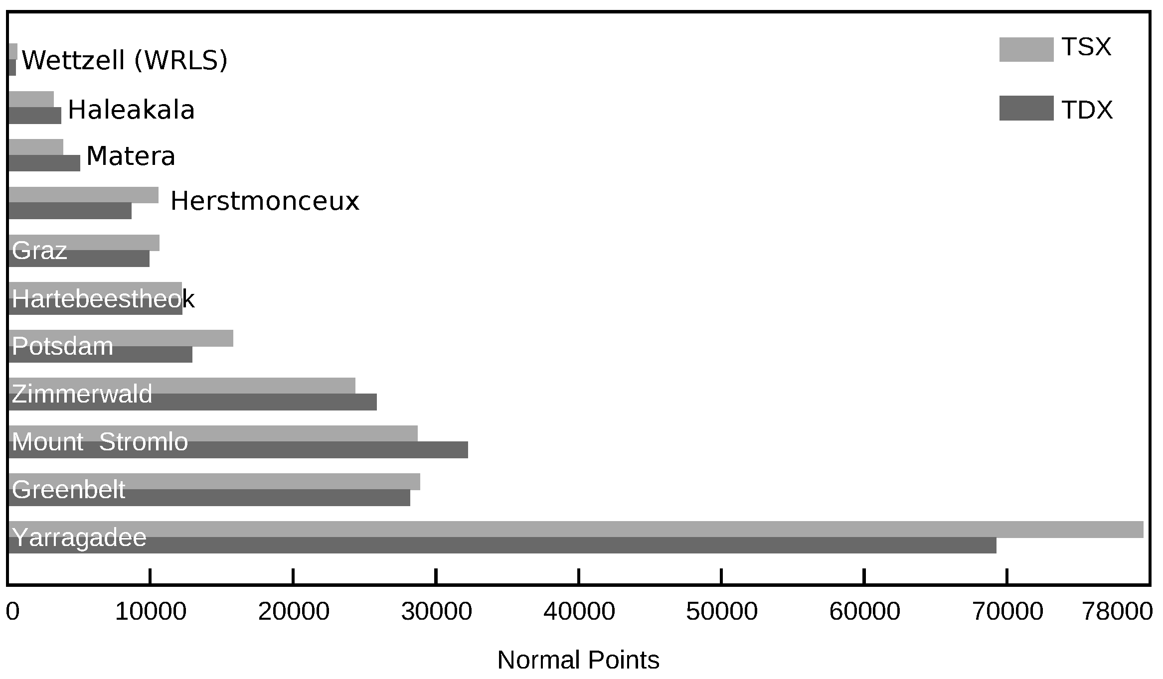
From 2012 to 2017, the satellites TSX and TDX acquired in total $1,033$ scenes for the five reflectors located at the geodetic stations. The imaging mode was the TerraSAR-X high resolution spotlight mode, which features an average resolution of 0.6 m by 1.1 m in slant range and azimuth, as well as a scene extent of approximately 5 km by 10 km [39]. Out of these acquisitions, 68 scenes had to be eliminated from the processing because they were rendered unusable by snow or water in the reflectors, which significantly reduce the signal backscatter. The degraded measurements are easily detected by computing the SCR from the CR point response in the radar image, and comparing it to the average SCR of the data series. In addition, 10 scenes were eliminated because of non-final alignments of the CRs or because of gross outliers at the decimeter level in the processed SAR residuals. The remaining scenes are distributed across several pass geometries that may be identified by the incidence angle at the CR at Doppler zero, see

Table 5. TerraSAR-X repeat pass geometries for the CRs at the geodetic observatories used in the study. The different geometries are identified by the incidence angles of the side-looking radar beams at zero Doppler.

CR	Pass Geometries [°]
${\mathrm{WTZ}}_A$	34, 46
${\mathrm{WTZ}}_D$	33, 45, 54
${\mathrm{OHI}}_A$	30, 38, 45
${\mathrm{OHI}}_D$	35, 43
${\mathrm{MET}}_D$	27, 37, 45

. Both satellites TSX and TDX captured data for all of the available reflectors, but in the case of TDX the majority of the data was acquired at GARS O’Higgins, while for TSX the data distribution across the sites is more homogeneous.

In order to center the SAR measurements and account for any unresolved biases caused by internal electronic delays of the SAR instrument, radar payloads are empirically calibrated against stable CRs with known reference coordinates. For the TerraSAR-X mission, the calibration was performed during the commissioning phase according to the initial requirements of 1 m [39,50], but because of our improvement in the TerraSAR-X range and azimuth measurements, we adopted the procedure to determine our own refined calibration constants for TSX and TDX [5,6]. The CR located at the Metsähovi station is used for this task. For the analysis presented in this study, the calibration constants were derived separately for both the standard PSOs and the enhanced orbit products, see

Table 6. Geometrical SAR calibration constants [m] of the TerraSAR-X mission derived from the Metähovi corner reflector for the different orbit solutions.

Solution	TSX		TDX
	Range	Azimuth	Range	Azimuth
PSO	$-0.3017$	$-0.0747$	$-0.2805$	$-0.0539$
ENH	$-0.2933$	$-0.0710$	$-0.2714$	$-0.0608$

. The changes in the calibration constants caused by the enhanced orbit product become as large as 1 cm. We may conclude that other uncompensated biases, e.g. from the orbit, are included in these constants in addition to the actual electronic instrument delays. 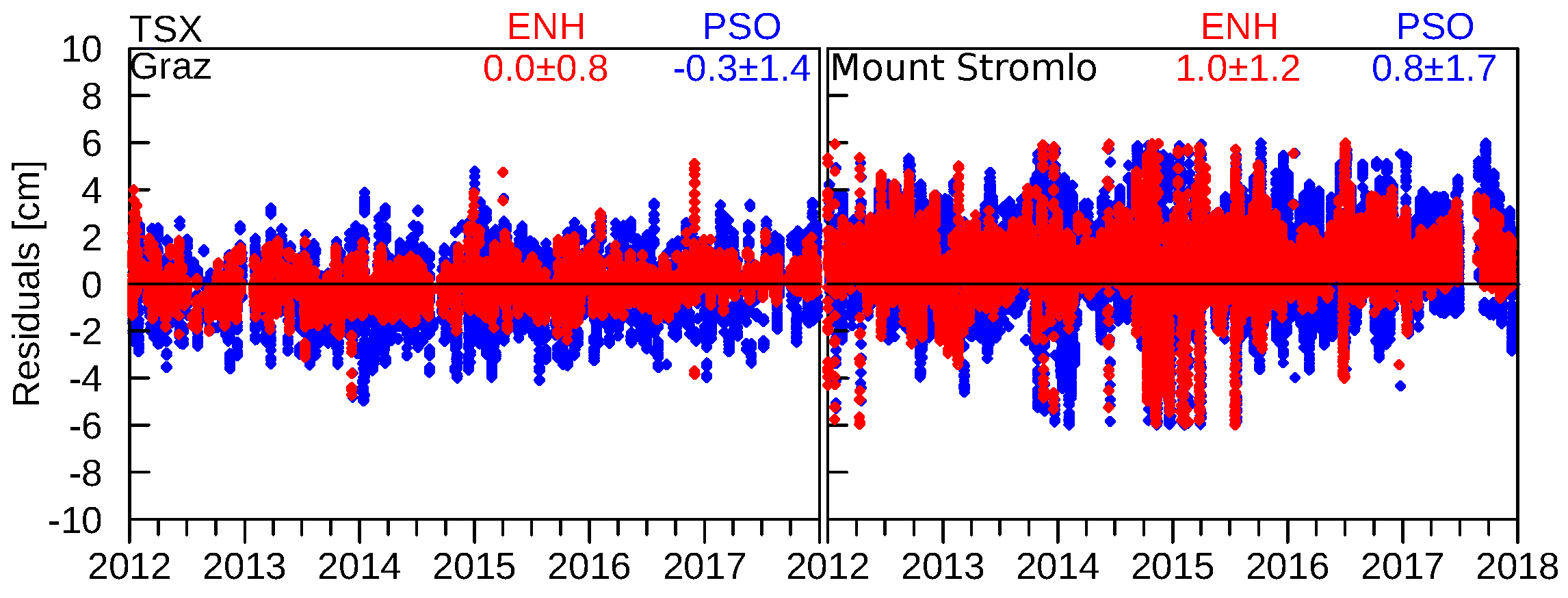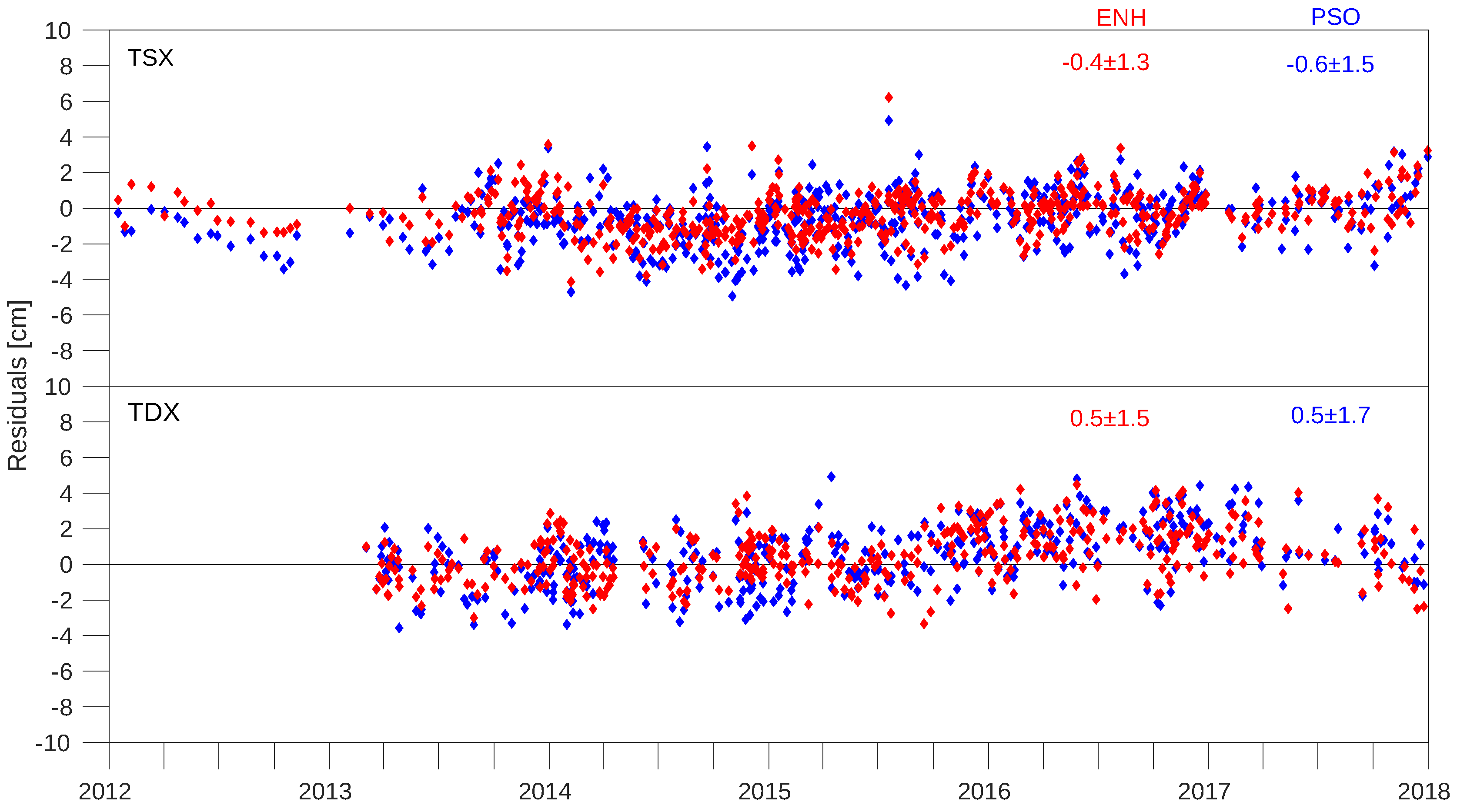This is also the reason why we decided to redetermine these constants after we introduced the refined modeling of the TerraSAR-X radar observations, see Section 4.2.1. Naturally, the remaining offset in the Metsähovi SAR residuals will become very small, but the offsets at the remaining four CRs can be used to judge the quality and the consistency of the SAR data and the two orbit products.

5. Validation Results and Discussion

5.1. Laser Ranging

For the 6 year period, and for both spacecrafts, TSX and TDX, the corresponding SLR residuals are shown in

Table 7. Satellite laser ranging residuals ($\overline{x}\pm {\sigma }_x$ [mm]) and amount of normal points ($N_{\mathrm{np}}$) for selected ILRS stations of the TSX and TDX orbit validation.

Station	TSX			TDX
	${\mathit{N}}_{\mathbf{np}}$	PSO	ENH	${\mathit{N}}_{\mathbf{np}}$	PSO	ENH
Graz	9966	$-2.7\pm 13.6$	$-0.7\pm \phantom{1}7.3$	9299	$-3.9\pm 14.0$	$-0.9\pm \phantom{1}7.9$
Greenbelt	27,060	$-11.8\pm 17.2$	$-7.5\pm 11.0$	26,413	$-10.4\pm 16.6$	$-6.8\pm 12.3$
Haleakala	2994	$0.1\pm 13.5$	$2.3\pm 10.4$	3507	$0.6\pm 14.4$	$3.1\pm 11.0$
Hartebeesthoek	11,425	$3.5\pm 20.0$	$6.8\pm 17.5$	11,460	$1.9\pm 21.0$	$5.4\pm 18.6$
Herstmonceux	9865	$-9.1\pm 12.0$	$-5.7\pm \phantom{1}6.8$	8127	$-9.7\pm 13.5$	$-6.2\pm \phantom{1}7.9$
Matera	3658	$-3.7\pm 14.2$	$-3.7\pm \phantom{1}9.2$	4743	$-8.5\pm 14.1$	$-5.1\pm 11.1$
Mount Stromlo	26,925	$8.0\pm 16.8$	$9.6\pm 12.0$	30,216	$7.7\pm 16.6$	$8.6\pm 12.7$
Potsdam	14,780	$-6.1\pm 14.3$	$-3.2\pm \phantom{1}9.5$	12,106	$-7.6\pm 14.4$	$-4.8\pm 10.0$
Wettzell	636	$4.0\pm 12.9$	$7.4\pm 10.1$	516	$-0.6\pm 13.0$	$3.1\pm 12.3$
Yarragadee	74,533	$0.8\pm 16.3$	$4.9\pm \phantom{1}8.3$	64,889	$1.2\pm 17.4$	$4.4\pm \phantom{1}9.7$
Zimmerwald	22,825	$-4.0\pm 12.9$	$-2.4\pm \phantom{1}8.2$	24,230	$-5.1\pm 14.2$	$-2.9\pm 10.7$
Total	204,667	$-1.5\pm 16.9$	$1.6\pm 11.4$	195,506	$-1.6\pm 17.5$	$1.2\pm 12.5$

. Figure 7 shows a time series of TSX and TDX satellite laser ranging residuals obtained from the two types of orbit solutions. In 2012, the series exhibits a data gap in January, which is caused by a planned outage of SLR tracking due to a spacecraft campaign. In general, the SLR residuals result in a mean offset of 2 mm over the 6 years of data. The standard deviation reaches up to 17 mm, which is reduced by 6 mm in the case of the enhanced solutions. The TDX series shows an increased amount of residual scatter in spring 2012, whereas both spacecrafts show similar patterns of larger residuals in mid 2014. Overall, the series do not show notable systematic variations with time.

Station-wise residual series help to identify systematic effects related to individual stations. As an example, Figure 8 shows station-wise SLR residuals series of two ILRS stations with totally different characteristics. The ILRS station Graz, Austria, exhibits no bias and a standard deviation of only 0.8 mm, whereas Mount Stromlo, Australia, shows a bias of 10 mm, along with a standard deviation of 12 mm for both the PSO and the ENH solutions. Outliers, which are most probably related to the station itself, are indicated by the vertically aligned dots stemming from specific passes. They can easily be identified in the series of Mount Stromlo, Australia. Contrary, the station in Graz, Austria, is almost free from such systematics. Offsets in station-wise SLR residuals hint to potential deficiencies in the knowledge of the SLR station coordinates and biases, as demonstrated in [10].

The SLR results listed in Table 7 demonstrate a 17.5 mm to 11.4 mm consistency across the selected stations. Basically, the SLR residuals constitute a measure of the one-dimensional orbit error. However, a simplified correlation to the associated 3-D position error is given by ${\sigma }_{\mathrm{pos}}=\sqrt{3{\sigma }_{\mathrm{SLR}}}$ [10], and amounts to 7.2 mm to 5.8 mm for the mentioned orbit products. Overall, the satellite laser ranging residuals in Table 7 result in a mean value of 1.6 mm and a standard deviation of 11.4 mm for TSX, which is similar to the TDX solutions of $1.2\pm 12.5$ mm. Compared to the results obtained with the precise science orbit products, the enhanced solutions show a 33 % reduction of the standard deviation, which is clear evidence for the improvements achieved with this solution. Depending on the elevation cut-off angle, the satellite laser ranging residuals are confined to a cone of 50°–80° with respect to the satellite’s nadir direction. Therefore, the SLR measurements are most sensitive to radial contributions of the orbit error.

5.2. Radar Ranging

For the SAR-based orbit validation, two independent sets of residuals can be analyzed, namely a set of residuals for the range and a set of residuals for the azimuth.

Table 8. SAR residuals ($\overline{x}\pm {\sigma }_x$ [mm]) and underlying number of data takes ($N_{\mathrm{dt}}$) for the stations with corner reflectors of the TSX and TDX orbit validation.

Station	TSX			TDX
	${\mathit{N}}_{\mathbf{dt}}$	PSO	ENH	${\mathit{N}}_{\mathbf{dt}}$	PSO	ENH
Wettzell Range	235	$-13.7\pm 13.1$	$-9.4\pm 10.3$	66	$-11.5\pm 12.9$	$-7.4\pm \phantom{1}8.1$
O’Higgins Range	135	$1.3\pm 16.3$	$1.9\pm 14.6$	305	$9.3\pm 15.7$	$7.6\pm 15.2$
Metsähovi Range	178	$-0.1\pm 11.2$	$0.3\pm 10.0$	36	$-0.4\pm 12.8$	$-0.3\pm 10.1$
Wettzell Azimuth	235	$10.7\pm 23.9$	$9.2\pm 21.9$	66	$5.2\pm 29.2$	$8.6\pm 24.6$
O’Higgins Azimuth	135	$18.0\pm 25.9$	$10.0\pm 23.7$	305	$-7.6\pm 28.2$	$0.1\pm 25.1$
Metsähovi Azimuth	178	$0.0\pm 17.6$	$0.0\pm 15.2$	36	$0.0\pm 18.2$	$0.0\pm 14.8$
Total Range	548	$-5.6\pm 15.1$	$-3.5\pm 12.5$	407	$5.1\pm 16.9$	$4.5\pm 14.9$
Total Azimuth	548	$9.0\pm 23.6$	$6.4\pm 20.9$	407	$-4.8\pm 28.0$	$1.4\pm 24.4$

lists the results for both types of observations as well as for TSX and TDX. The findings show a very good agreement regarding the standard deviations across the stations and the two orbit solutions tested. With the PSOs, the standard deviation of the SAR ranging is in the order of 15 mm, while for the ENH solution we see an improvement to 10 mm. Note that the standard deviations of the GARS O’Higgins range results are larger when compared to standard deviations of the other two stations hosting CRs. Part of the explanation may be found in the different CR sizes, i.e., 0.7 m versus 1.5 m. The estimates presented earlier in Table 3 indicate a drop in the range localization precision by approximately 5 mm for the smaller reflectors. Moreover, there is a slight tendency towards the positive range for the TDX range data of GARS O’Higgins between mid 2016 to mid 2017, see Figure 9, which is present in both orbit solutions. The effect also has an impact on the mean and standard deviations computed for this site. The much sparser data of TSX for GARS O’Higgins indicate a similar behavior; thus we think it is related to CR installations at GARS O’Higgins, and it is also the reason why there is less improvement in the overall TDX results and the ENH orbit solution, because the data is dominated by the acquisitions at GARS O’Higgins.

Regarding the results in azimuth, one immediately notices the increase in the standard deviations by approximately a factor of 1.5 when compared to range. Once more there is an impact of the smaller CRs of GARS O’Higgins, resulting in azimuth standard deviations of 25 mm. However, for Wettzell we would expect the azimuth results to be closer to the 16 mm azimuth standard deviation observed at Metsähovi. Instead, the Wettzell azimuth results are almost identical to the findings of GARS O’Higgins. The main driver for the TerraSAR-X quality in azimuth is the temporal link between the absolute time provided by the MosaicGNSS receiver and the SAR payload. The limit of the link is considered to be approximately 1 microsecond once the significant digits truncated by the on-board data quantization have been restored [44]. An uncertainty of 1 microsecond translates into approximately 7 mm in azimuth when taking into account the average TerraSAR-X orbit velocity of 7683 m/s. However, the azimuth results we obtain from the experiments show a larger noise than we would expect from this consideration, and therefore further investigations on the SAR payload and the processing are required to identify their possible cause.

The detailed station results for Wettzell and GARS O’Higgins are shown in Figure 9. The plots confirm that the larger azimuth standard deviations are indeed due to an increase in the azimuth noise, and that the range is the more sensitive measurement of the SAR. There are slight temporal variations visible in the SAR range results of both orbit solutions, which are similar to the variations found in the temporal series of the SLR residuals, see Figure 8. Most prominent is the aforementioned systematic effect in the range for the TDX data at GARS O’Higgins. However, because of the smaller amount of stations in the SAR analysis, there is no definite conclusion whether they are due to SAR payloads or because of local signals related to the CR sites. As a summary, Figure 10 provides a comprehensive view of all the SAR ranging residuals for the ENH and the PSO orbit solutions. The reason for the small number of TSX data and the lack of data for TDX in the first year lies in the setup of the CR sites. During the first year, only one reflector was available at Wettzell, Germany, which was covered solely by the TDX spacecraft. In spite of the details discussed for the solutions of the individual CR sites, these combined plots confirm the very good overall consistency of both TSX and TDX across the sites, as well as the high quality of the ENH orbit solution.

5.3. Position Offset Estimates

The derived SLR range residuals give a measure of the radial accuracy. Whenever the scope is on physical effects or on the accelerations in a certain direction, the SLR-based position offset estimates can improve the interpretation. Therefore, the laser measurements are further utilized for an estimation of spacecraft position offsets in radial, along-, and cross-track directions. The applied setup of SLR preprocessing and data screening is identical to the approach described above, and the analysis period also covers 6 years and both orbit solutions for each of the spacecrafts. The values listed in the results are based on monthly averages.

In principle, the SAR residuals in range and azimuth allow for the same position offset analysis. However, the permanently right-looking nature of the SAR instruments yields radar ranges that basically cover only one cross-direction of the orbit, for which the ranges have an angular separation of approximately 15 to 20 degrees, see the pass geometries given in Table 5. The advantage of measuring all the pass geometries and the considerably larger amount of tracking data enables the SLR to reliably determine the monthly position offsets for all three directions with an estimated accuracy at the sub-millimeter level. In contrast, our tests with the SAR residuals showed estimated accuracies for the cross-track and radial position offsets at the centimeter level, and an accuracy at the millimeter level for the along-track position offsets. Because of these results, we decided to keep the SAR data in the geometry of range and azimuth, but to apply a monthly averaging to preserve the comparison with the SLR-based position offsets. Prior to the monthly averaging, the full rate SAR residuals of range and azimuth were reduced by global $2\sigma$ tests. The tests eliminate approximately 4% of the SAR residuals in the TSX and TDX data series, which exceed the thresholds of two times the estimated standard deviations. They also remove the few remaining outliers in the range and azimuth residuals (see for instance the ranging residuals shown in Figure 10) that would otherwise distort the monthly mean estimates.

Table 9. Monthly position offsets in radial, along-track and cross-track derived from satellite laser ranging, and monthly range and azimuth offsets derived from the SAR measurements. Obtained from the precise science (PSO) and the enhanced orbit solutions (ENH) for TSX and TDX ($\overline{x}\pm {\sigma }_x$ [mm]).

Type	Orbit	TSX			TDX
		Radial	Along-Track	Cross-Track	Radial	Along-Track	Cross-Track
SLR	PSO	$-1.6\pm 2.8$	$2.1\pm 4.1$	$-11.9\pm 8.1$	$-2.3\pm 3.4$	$2.7\pm 3.4$	$-10.0\pm 8.0$
SLR	ENH	$2.4\pm 2.7$	$0.4\pm 3.2$	$0.5\pm 1.9$	$1.5\pm 3.1$	$1.8\pm 2.7$	$-0.1\pm 1.9$
			azimuth	range		azimuth	range
SAR	PSO		$6.7\pm 8.9$	$-6.8\pm 8.2$		$-7.2\pm 12.6$	$5.1\pm 10.6$
SAR	ENH		$5.4\pm 7.9$	$-3.4\pm 6.9$		$\phantom{-}1.4\pm \phantom{1}9.2$	$3.1\pm \phantom{1}8.3$

comprises the estimated offset values that are associated with the time series visualized in Figure 11 and Figure 12. The SLR analysis shows average monthly offsets well below 12 mm in the spacecraft’s radial, along-, and cross-track direction. The cross-track component underlines the clear advantage of the ENH solutions, for which the remaining mean values are reduced from one centimeter to less than one millimeter. The induced shift between the PSO and the ENH solutions is similar for both spacecrafts and can bee seen in Figure 11. The along-track component is also slightly improved. The monthly SAR azimuth results are comparable to the SLR along-track estimates and thus we decided to place them side by side in Table 9. The comparison of both results indicate that the SLR along-track offsets are approximately 2–3 times more reliable than the 5–7 mm offsets found for SAR azimuth, but one should also take into account the large differences in the underlying data, namely about 2000 NPs per month for the SLR versus the 5–10 SAR acquisitions per month at the CR sites. Nevertheless, the improvement of the ENH solutions is also clearly visible in the SAR azimuth offsets, especially in the mean value of TDX that is reduced from $-7.2$ mm to 1.4 mm. The monthly SAR range offsets given in Table 9 confirm the findings for the ENH solutions. Again we observe a reduction of both the mean values and the standard deviations well below 10 mm. Note that the slightly larger numbers for TDX are due to the systematics in the GARS O’Higgins data during the years 2016 and 2017, which was already discussed in the previous section and can be seen once more in Figure 12. In summary, we can conclude that both techniques agree in their monthly assessment of the TerraSAR-X orbit solutions.

6. Conclusions and Outlook

Independent distance measurements to/from satellites are perfectly suited to orbit validation. SAR and SLR are two active techniques, which allow measuring the distance to a point target, known as a LRRs onboard the satellite in case of laser, or CR on ground in case of radar observations. Both techniques require availability of precise coordinates, which is an important pre-condition. Taking into account 11 stations from the ILRS network for SLR, and 3 stations with trihedral CRs for the SAR ranging, orbit solutions of the spacecrafts TSX and TDX are thoroughly analyzed within the 2012–2017 period. Two types of orbit solutions are computed at GSOC/DLR and employed for comparison: the operational PSO products, and enhanced orbit solutions, which incorporate refined dynamical models, and the GPS integer ambiguity fixing. The validation using the SLR residuals is based on differences between observed and modeled station-to-satellite ranges, and demonstrates a consistency of the TSX orbit products with the optical measurements at a level of 12–17 mm. Corresponding radar ranging residuals are obtained from differences between observed and modeled satellite-to-station ranges, are consistent at a level of 18–26 mm. The results obtained from TDX solutions are similar. Regarding the number of available tracking data, $400,173$ SLR normal points are available for the spacecrafts TSX and TDX within the 6 years, whereas 1910 SAR measurements in range and azimuth are available in the same period. The outstanding number of SLR tracking points is because of the high tracking priority of the spacecrafts.

The number of available data limits the capabilities of radar ranging to estimate spacecraft offsets. In case of SLR, a 10-mm shift in cross-track direction can be observed when switching from the PSO to the enhanced orbit solutions. For instance, such offsets can be utilized for identifying center-of-gravity position corrections, or SLR station corrections [10,19]. Similar to the SLR, the SAR range residuum also shows a shift of several millimeters.

Regarding the abilities of both validiation techniques, the following conclusions can be stated. The SLR depends on weather and cloud conditions, whereas SAR is principally free of these limitations. On the other hand, SAR is limited by the corrections for the atmospheric path delays, in particular for the ionosphere, because the range measurements behave like single-frequency microwave observations. The SLR may observe all passes from horizon to horizon, whereas conventional spaceborne SAR payloads observe only in a fixed right-looking (or left-looking) direction and provide only the observations at the instant of zero Doppler. SLR needs dedicated stations while the SAR satellites have global access, provided that passive CRs are available.

Especially for radar satellite missions, the proposed SAR validation paves the way for another, independent orbit validation tool, which is of particular interest for the Sentinel-1 mission, because these spacecrafts are not equipped with LRRs [51]. Since the SAR-based validation technique requires less infrastructure when compared to an SLR station, an extension of the ground corner reflector network is envisaged.

References

1. Werninghaus, R.; Buckreuss, S. The TerraSAR-X Mission and System Design. IEEE Trans. Geosci. Remote Sens. 2010, 48, 606–614. [Google Scholar] [CrossRef] [Green Version]
2. Moreira, A.; Krieger, G.; Hajnsek, I.; Hounam, D.; Werner, M.; Riegger, S.; Settelmeyer, E. TanDEM-X: A TerraSAR-X Add-On Satellite for Single-Pass SAR Interferometry. IEEE Trans. Geosci. Remote Sens. 2004, 2, 1000–1003. [Google Scholar]
3. Eineder, M.; Minet, C.; Steigenberger, P.; Cong, X.; Fritz, T. Imaging geodesy—Toward centimeter-level ranging accuracy with TerraSAR-X. IEEE Trans. Geosci. Remote Sens. 2011, 49, 661–671. [Google Scholar] [CrossRef]
4. Schubert, A.; Jehle, M.; Small, D.; Meier, E. Mitigation of atmospheric perturbations and solid Earth movements in a TerraSAR-X time-series. J. Geod. 2012, 86, 257–270. [Google Scholar] [CrossRef]
5. Gisinger, C.; Balss, U.; Pail, R.; Zhu, X.; Montazeri, S.; Gernhardt, S.; Eineder, M. Precise Three-Dimensional Stereo Localization of Corner Reflectors and Persistent Scatterers with TerraSAR-X. IEEE Trans. Geosci. Remote Sens. 2015, 53, 1782–1802. [Google Scholar] [CrossRef]
6. Balss, U.; Gisinger, C.; Eineder, M. Measurements on the Absolute 2-D and 3-D Localization Accuracy of TerraSAR-X. Remote Sens. 2018, 10, 656. [Google Scholar] [CrossRef]
7. Krieger, G.; Moreira, A.; Fiedler, H.; Hajnsek, I.; Werner, M.; Younis, M.; Zink, M. TanDEM-X: A Satellite Formation for High-Resolution SAR Interferometry. IEEE Trans. Geosci. Remote Sens. 2007, 45, 3317–3341. [Google Scholar] [CrossRef] [Green Version]
8. Yoon, Y.; Eineder, M.; Yague-Martinez, N.; Montenbruck, O. TerraSAR-X Precise Trajectory Estimation and Quality Assessment. IEEE Trans. Geosci. Remote Sens. 2009, 47, 1859–1868. [Google Scholar] [CrossRef]
9. Tapley, B.D.; Schutz, B.E.; Eanes, R.J. Satellite laser ranging and its applications. Celest. Mech. 1985, 37, 247–261. [Google Scholar] [CrossRef]
10. Arnold, D.; Montenbruck, O.; Hackel, S.; Sośnica, K. Satellite Laser Ranging to Low Earth Orbiters—Orbit and Network Validation. J. Geod. 2018, 1–20. [Google Scholar] [CrossRef]
11. Balss, U.; Cong, X.; Brcic, R.; Rexer, M.; Minet, C.; Breit, H.; Eineder, M.; Fritz, T. High precision measurement on the absolute localization accuracy of TerraSAR-X. In Proceedings of the 2012 IEEE International Geoscience and Remote Sensing Symposium (IGARSS), Munich, Germany, 22–27 July 2012; pp. 1625–1628. [Google Scholar]
12. Kahle, R.; Kazeminejad, B.; Kirschner, M.; Yoon, Y.; Kiehling, R.; D’Amico, S. First In-Orbit Experience of TerraSAR-X flight dynamic operations. In Proceedings of the 20th International Symposium on Space Flight Dynamics, Annapolis, MD, USA, 24–28 September 2007. [Google Scholar]
13. Buckreuss, S.; Balzer, W.; Mühlbauer, P.; Werninghaus, R.; Pitz, W. The TerraSAR-X satellite project. In Proceedings of the 2003 IEEE International Geoscience and Remote Sensing Symposium, Toulouse, France, 21–25 July 2003; Volume 5, pp. 3096–3098. [Google Scholar]
14. Eineder, M.; Runge, H.; Boerner, E.; Bamler, R.; Adam, N.; Schättler, B.; Breit, H.; Suchandt, S. SAR interferometry with TerraSAR-X. In Proceedings of the FRINGE 2003 Workshop, Frascati, Italy, 1–5 December 2000. [Google Scholar]
15. Montenbruck, O.; Kroes, R. In-flight performance analysis of the CHAMP BlackJack GPS Receiver. GPS Solut. 2003, 7, 74–86. [Google Scholar] [CrossRef]
16. Montenbruck, O.; Yoon, Y.; Ardaens, J.S.; Ulrich, D. In-Flight Performance Assessment of the Single Frequency MosaicGNSS Receiver for Satellite Navigation. In Proceedings of the 7th International ESA Conference on Guidance, Navigation and Control Systems, County Kerry, Ireland, 2–5 June 2008. [Google Scholar]
17. Wermuth, M.; Montenbruck, O.; van Helleputte, T. GPS High Precision Orbit Determination Tools (GHOST). In Proceedings of the 4th International Conference on Astrodynamics Tools and Techniques, Madrid, Spain, 3–6 May 2010. [Google Scholar]
18. Hackel, S.; Montenbruck, O.; Steigenberger, P.; Balss, U.; Gisinger, C.; Eineder, M. Model improvements and validation of TerraSAR-X precise orbit determination. J. Geod. 2017, 91, 547–562. [Google Scholar] [CrossRef]
19. Montenbruck, O.; Hackel, S.; Jäggi, A. Precise orbit determination of the Sentinel-3A altimetry satellite using ambiguity-fixed GPS carrier phase observations. J. Geod. 2017. [Google Scholar] [CrossRef]
20. Loyer, S.; Perosanz, F.; Mercier, F.; Capdeville, H.; Marty, J.C. Zero-difference GPS ambiguity resolution at CNES-CLS IGS Analysis Center. J. Geod. 2012, 86, 991–1003. [Google Scholar] [CrossRef]
21. Schmid, R.; Dach, R.; Collilieux, X.; Jäggi, A.; Schmitz, M.; Dilssner, F. Absolute IGS antenna phase center model igs08.atx: status and potential improvements. J. Geod. 2016, 90, 343–364. [Google Scholar] [CrossRef]
22. Altamimi, Z.; Rebischung, P.; Métivier, L.; Collilieux, X. ITRF2014: A new release of the International Terrestrial Reference Frame modeling nonlinear station motions. J. Geophys. Res. Solid Earth 2016, 121, 6109–6131. [Google Scholar] [CrossRef]
23. Wu, J.; Wu, S.; Hajj, G.; Bertiger, W.; Lichten, S. Effects of antenna orientation on GPS carrier phase. Manuscr. Geod. 1993, 18, 91–98. [Google Scholar]
24. Mayer-Gürr, T.; Pail, R.; Schuh, W.D.; Kusche, J.; Baur, O.; Jäggi, A. The new combined satellite only model GOCO03s. In Proceedings of the International Symposium on Gravity, Geoid and Height Systems GGHS2012, Venice, Italy, 9–12 October 2012. [Google Scholar]
25. Eanes, R.J.; Bettadpur, S. The CSR 3.0 Global Ocean Tide Model: Diurnal and Semi-Diurnal Ocean Tides from TOPEX/POSEIDON Altimetry; Technical Report 6; Center for Space Research, University of Texas at Austin: Austin, TX, USA, 1995. [Google Scholar]
26. Priestley, K.J.; Smith, G.L.; Thomas, S.; Cooper, D.; Lee, R.B.; Walikainen, D.; Hess, P.; Szewczyk, Z.P.; Wilson, R. Radiometric Performance of the CERES Earth Radiation Budget Climate Record Sensors on the EOS Aqua and Terra Spacecraft through April 2007. J. Atmos. Ocean. Technol. 2011, 28, 3–21. [Google Scholar] [CrossRef]
27. Picone, J.M.; Hedin, A.E.; Drob, D.P.; Aikin, A.C. NRLMSISE-00 empirical model of the atmosphere: Statistical comparisons and scientific issues. J. Geophys. Res. 2002, 107, 1468. [Google Scholar] [CrossRef]
28. Shampine, L.F.; Gordon, M.K. Computer Solution of Ordinary Differential Equations: The Initial Value Problem; W.H. Freeman & Co., Ltd.: San Francisco, CA, USA, 1975. [Google Scholar]
29. Pearlman, M.R.; Degnan, J.J.; Bosworth, J.M. The International Laser Ranging Service. Adv. Space Res. 2002, 30, 135–143. [Google Scholar] [CrossRef]
30. Neubert, R.; Grunwaldt, L.; Neubert, J. The Retro-Reflector for the CHAMP Satellite: Final Design and Realization. In Proceedings of the 11th International Workshop on Laser Ranging, Deggendorf, Germany, 21–25 September 1998. [Google Scholar]
31. International Laser Ranging Service. SLRF2014 Station Coordinates. 2017. Available online: ftp://ftp.cddis.eosdis.nasa.gov/pub/slr/products/resource/SLRF2014_POS+VEL_2030.0_170605.snx (accessed on 8 June 2017).
32. Ray, R. A Global Ocean Tide Model from TOPEX/Poseidon Altimeter: GOT99; Tm-209478; NASA Technical Memorandum; NASA: Greenbelt, MA, USA, 1999.
33. Mendes, V.; Pavlis, E. High-accuracy zenith delay prediction at optical wavelengths. Geophys. Res. Lett. 2004, 31, L14602. [Google Scholar] [CrossRef]
34. Pavlis, E. SLRF2008: The ILRS reference frame for SLR POD contributed to ITRF2008. In Proceedings of the 2009 Ocean Surface Topography Science Team Meeting, Buellton, CA, USA, 19 June 2009. [Google Scholar]
35. International Association of Geodesy. International Laser Ranging Service Mission Priorities as of December 25, 2017. Available online: https://ilrs.cddis.eosdis.nasa.gov/missions/mission_operations/priorities/index.htmll (accessed on 25 December 2017).
36. International Laser Ranging Service. TerraSAR-X. 2015. Available online: http://ilrs.gsfc.nasa.gov/missions/satellite_missions/current_missions/tsar_general.html (accessed on 15 January 2015).
37. Cumming, I.G.; Wong, F.H. Digital Processing of Synthetic Aperture Radar Data; Artech House: Norwood, MA, USA, 2005. [Google Scholar]
38. Breit, H.; Fritz, T.; Balss, U.; Lachaise, M.; Niedermeier, A.; Vonavka, M. TerraSAR-X SAR Processing and Products. IEEE Trans. Geosci. Remote Sens. 2010, 48, 727–740. [Google Scholar] [CrossRef]
39. TerraSAR-X Ground Segment Basic Product Specification Document. TX-GS-DD-3302, v1.9, 09.10.2014. 2013. Available online: http://sss.terrasar-x.dlr.de (accessed on 26 March 2018).
40. Döring, B.; Schwerdt, M.R.B. TerraSAR-X Calibration Ground Equipment. In Proceedings of the Wave Propagation in Communication, Microwaves Systems and Navigation (WFMN), Chemnitz, Germany, 4–5 July 2007. [Google Scholar]
41. Petit, G.; Luzum, B. (Eds.) IERS Conventions (2010); Verlag des Bundesamts für Kartographie und Geodäsie: Frankfurt, German, 2010; Available online: http://tai.bipm.org/iers/conv2010/conv2010.html (accessed on 26 March 2018).
42. Stein, S. Algorithms for Ambiguity Function Processing. IEEE Trans. Acoust. Speech Signal Process. 1981, ASSP-29, 588–599. [Google Scholar] [CrossRef]
43. Bamler, R.; Eineder, M. Accuracy of Differential Shift Estimation by Correlation and Split-Bandwidth Interferometry for Wideband and Delta-k SAR Systems. IEEE Geosci. Remote Sens. Lett. 2005, 2, 151–155. [Google Scholar] [CrossRef]
44. Balss, U.; Breit, H.; Fritz, T.; Steinbrecher, U.; Gisinger, C.; Eineder, M. Analysis of Internal Timings and Clock Rates of TerraSAR-X. In Proceedings of the 2014 IEEE International Geoscience and Remote Sensing Symposium (IGARSS), Quebec City, QC, Canada, 13–18 July 2014; pp. 2671–2674. [Google Scholar]
45. Byram, S.; Hackman, C.; Tracey, J. Computation of a High-Precision GPS-Based Troposphere Product by the USNO. In Proceedings of the 24th international technical meeting of the satellite division of the institute of navigation (ION GNSS 2011), Portland, OR, USA, 20–23 September 2011; pp. 572–578. [Google Scholar]
46. Altamimi, Z.; Collilieux, X.; Métivier, L. ITRF2008: An improved solution of the international terrestrial reference frame. J. Geod. 2011, 85, 457–473. [Google Scholar] [CrossRef] [Green Version]
47. Schlüter, W.; Zernecke, R.; Becker, S.; Klügel, T.; Thaller, D. Local Ties between the Reference Points at the Fundamentalstation Wettzell. In Proceedings of the IERS Workshop on Site Co-Location, Matera, Italy, 23–24 October 2003; IERS Technical Note 33. Richter, B., Dick, W.R., Schwegmann, W., Eds.; pp. 64–70. Available online: https://www.iers.org/IERS/EN/Publications/publications.html (accessed on 26 March 2018).
48. Klügel, T.; Mähler, S.; Schade, C. Ground Survey and Local Ties at the Geodetic Observatory Wettzell. In Proceedings of the 17th International Workshop on Laser Ranging, Bad Koetzting, Germany, 16–20 May 2011; Available online: https://cddis.nasa.gov/lw17/ (accessed on 26 March 2018).
49. International Earth Rotation and Reference Systems Service (IERS). The International Terrestrial Reference Frame (ITRF). 2018. Available online: https://www.iers.org/IERS/EN/DataProducts/ITRF/itrf.html (accessed on 26 March 2018).
50. Schwerdt, M.; Bräutigam, B.; Bachmann, M.; Döring, B.; Schrank, D.; Gonzalez, J.H. Final TerraSAR-X Calibration Results Based on Novel Efficient Methods. IEEE Trans. Geosci. Remote Sens. 2010, 48, 677–689. [Google Scholar] [CrossRef]
51. Peter, H.; Jäggi, A.; Fernández, J.; Escobar, D.; Ayuga, F.; Arnold, D.; Wermuth, M.; Hackel, S.; Otten, M.; Simons, W.; et al. Sentinel-1A—First precise orbit determination results. Adv. Space Res. 2017, 60, 879–892. [Google Scholar] [CrossRef]
Figure 1. Illustration of TerraSAR-X with selected optical and radar payload for orbit validation.
Remotesensing 10 00762 g001
Figure 2. Selected stations of ground network, utilized for orbit validation. Radar corner reflectors, utilized by the SAR analysis, are indicated by triangles; the selected ILRS stations for SLR by dots.
Remotesensing 10 00762 g002
Figure 3. Laser retro reflector array of TSX (TerraSAR-X) and TDX(TanDEM-X) (courtesy GFZ Potsdam).
Remotesensing 10 00762 g003
Figure 4. Number of accepted normal points for selected ILRS stations between 2012 and 2017.
Remotesensing 10 00762 g004
Figure 5. Corner reflectors (CRs) at geodetic observatories. CR with 0.7 m inner leg dimension at GARS O’Higgins (left), and CRs with 1.5 m inner leg dimension at Wettzell (middle) and at Metsähovi (right).
Remotesensing 10 00762 g005
Figure 6. Zero-Doppler geometry of a SAR acquisition in the ITRF for a corner reflector at X r and a satellite pass given by the dashed line.
Remotesensing 10 00762 g006
Figure 7. Satellite laser ranging residuals obtained for the TSX and TDX enhanced orbit solutions (ENH, red) and the precise science orbits (PSO, blue).
Remotesensing 10 00762 g007
Figure 8. Satellite laser ranging residuals of TSX orbit solutions from the ILRS stations Graz, Austria, and Mount Stromlo, Australia.
Remotesensing 10 00762 g008
Figure 9. TerraSAR-X range and azimuth residuals derived from the Wettzell corner reflectors (top) and the GARS O’Higgins corner reflectors (bottom).
Remotesensing 10 00762 g009
Figure 10. Radar ranging residuals obtained for TSX and TDX enhanced (ENH, red) and precise science orbit (PSO, blue) orbit solutions.
Remotesensing 10 00762 g010
Figure 11. Series of monthly-derived position offsets obtained from satellite laser ranging for the enhanced (ENH) and the precise science orbits (PSOs) of the TerraSAR-X mission.
Remotesensing 10 00762 g011
Figure 12. Series of monthly-derived SAR range and azimuth residuals for the enhanced (ENH) and the precise science orbits (PSOs) of the TerraSAR-X mission.
Remotesensing 10 00762 g012