Article

Temporal—Spatial Changes in Vegetation Coverage under Climate Change and Human Activities: A Case Study of Central Yunnan Urban Agglomeration, China

1
College of Landscape Architecture and Horticulture Science, Southwest Forestry University, Kunming 650224, China
2
Southwest Landscape Engineering Technology Research Center of National Forestry and Grassland Administration, Kunming 650224, China
*
Author to whom correspondence should be addressed.
Sustainability 2024, 16(2), 661; https://doi.org/10.3390/su16020661
Submission received: 21 November 2023 / Revised: 21 December 2023 / Accepted: 9 January 2024 / Published: 11 January 2024

Abstract

:
Analyzing vegetation cover provides a basis for detecting ecological and environmental health in urban areas. We analyzed the temporal and spatial changes in vegetation cover using NDVI data from the central Yunnan urban agglomeration (CYUA). The dimidiate pixel model (DPM) and intensity analysis were used to study changes at three levels: time intervals, category, and transition. Analysis of time series data from 1990–2020 using the Theil–Sen Median with Mann–Kendal test identified the overall trends. Geodetector explored the relationship between natural and human factors in vegetation cover change. The CYUA’s vegetation cover gradually decreases from west to east and south to north, with middle–high and high vegetation occupying over 55%. During 1990–2020, significant improvement was observed in the east and north regions, with an increase of 22.49%. The anthropogenic core area showed severe degradation with nearly 1.56% coverage. The transformation intensity of middle vegetation coverage was dominant from 1990–2010 but was replaced by middle–high vegetation coverage from 2010–2020. Meanwhile, high vegetation coverage became the most prominent gains target, and the conversion of middle–high to high vegetation showed a system tendency to exceed the average in absolute number and relative intensity. Spatial and temporal differences in vegetation cover were mostly affected by land cover (q = 0.4726, p < 0.001), and the most influential topographic factor was the slope (q = 0.1491, p < 0.001). The impact of human activities has increased to 16%, double that of 2000. The CYUA’s vegetation cover improved more than it degraded, but required site-specific forest management due to human activities.

1. Introduction

The World Cities Report 2022 sheds light on the ongoing trend of urbanization [1], particularly in developing nations with rapid urban growth. As cities expand, their impact on surface form and microclimate becomes increasingly noticeable, with green spaces in urban areas particularly vulnerable to human and economic activity [2,3]. There are various methods used to assess green spaces in urban areas, such as accessibility [4], green-looking ratio [5], landscape patterns [6], land use/land cover [7], and ecosystem services [8]. However, vegetation cover remains the most crucial aspect of terrestrial ecosystems and a critical factor for characterizing land surface cover [9]. Alterations in vegetation coverage can reveal the ecological health of a region and help identify the environmental quality of its green spaces. Therefore, evaluating and preserving urban green spaces is crucial, as they offer numerous benefits including enhanced mental and physical health, biodiversity, and climate regulation.
Fractional vegetation cover (FVC) is a significant factor used to assess the condition of surface vegetation [10]. It is defined as the ratio of vertically projected area covered by vegetation to overall surface area [11,12]. Research on vegetation coverage is usually combined with the analysis of vegetation structure, remote sensing images, ecosystem services, land cover, and urban expansion [13,14]. With the development of remote sensing and satellite imaging technologies, high-definition images provide new research materials. Remote sensing data, representing vegetation cover, has been widely used to calculate the vegetation index in order to quantitatively detect vegetation growth [15,16], seasonal change, spatial pattern characteristics, and influencing factors. Vegetation indices such as NDVI and EVI are commonly used to study plant growth. NDVI can be used in all stages of plant growth, while EVI is more effective in areas with a lot of chlorophyll and flat terrain [17,18]. NDVI is considered one of the best vegetation indices because it eliminates most of the variations caused by factors such as sun angle, instrument calibration, topography, cloud shadow, and atmosphere. This makes it a more accurate measure of vegetation growth [19,20]. There are various methods available for deriving vegetation coverage, such as relative vegetation abundance (RA) algorithms, spectral mixture analysis (SMA) algorithms, spectral-based supervised classification algorithms, physically-based models, machine learning algorithms, and other methods [21]. One of the most widely used algorithms for RA is the dimidiate pixel model (DPM), which is a linear mixed model. It is preferred due to its simple algorithm and effective simulation [17,22]. Numerous studies have utilized NDVI to examine the correlation between vegetation and urban environment at various levels, ranging from global [23] to national [24] and regional scales [25]. For urban-scale research, recent studies have used NDVI to characterize urban green space with better results than land cover [26]. Therefore, it is urgent to increase the study of green space in urban areas from the perspective of vegetation cover.
Vegetation coverage analysis can be effectively evaluated through the examination of temporal and spatial transformations. One approach to achieve spatial alterations involves the utilization of land use/cover transfer and spatial autocorrelation methods [27,28]. Meanwhile, linear regression analysis can be employed to forecast transformation trends through time [29,30]. It is widely acknowledged that both climate change and human activities are the primary driving forces that impact vegetation cover [31,32]. Researchers have focused on characterizing, identifying, and exploring the impact of driving factors on vegetation cover [33,34]. Partial correlation analysis, t-tests, residual analysis, and the geodetector model are some of the methods used to study the driving factors. However, it is important to note that correlation or regression methods may only reflect results if there is linearity between the factors and driving forces [35]. In contrast, the geodetector model can quantify the nonlinear effects of multiple influencing factors and interactions, meaning it overcomes the limitations of traditional methods [36]. Therefore, it has become an effective tool to quantify the factors influencing vegetation cover changes.
The central Yunnan urban agglomeration (CYUA) is a newly developed urban area in China which is considered the core area for the development of Yunnan Province; by the end of 2022, it had an overall urbanization level of 58.94%, which is higher than the provincial average of 53% [37,38]. It is known for its rich botanical resources and is also a hub for economic and cultural activities. However, extreme climate and intensified human activities in recent years have affected the vegetation coverage level in the region. The increasingly dry and warm climate has affected the growth of vegetation, and human economic construction activities continue to change the stability of vegetation [39]. With a unique topography ranging from tropical rainforests to high-altitude meadows, the CYUA provides a valuable opportunity to study the impact of climate change on vegetation cover. However, rapid urbanization has resulted in significant environmental challenges, including air and water pollution, deforestation, and land use changes. Given the region’s rich natural resources, monitoring environmental quality is essential to prevent ecological crises. This study serves as a theoretical basis for monitoring environmental quality changes in the region and developing sustainable development strategies to mitigate the negative impact of urbanization on the environment.
This paper, based on the NDVI data of the central Yunnan urban agglomeration (CYUA), used the dimidiate pixel model, intensity analysis, and intensity map methods to analyze the spatial and temporal changes in vegetation cover at three levels: time intervals, category, and transition. The Theil–Sen Median trend analysis was integrated with a Mann–Kendal analysis to analyze the characteristics of the overall change trends in vegetation coverage based on the time series data from 1990 to 2020. In addition, we used the geodetector model to explore the relationship between natural and human factors that affect vegetation cover change in the CYUA. The geodetector model is an effective tool for analyzing the relative importance and interaction between various factors [40]. This analysis provides a comprehensive understanding of the factors contributing to vegetation changes in the CYUA.
The results of this study will provide valuable insights into the construction and ecological management of green spaces in the CYUA. We anticipate that the findings will support sustainable development and ecological conservation efforts in the CYUA. The following questions need to be addressed: (a) What was the vegetation cover of the CYUA between 1990 and 2020? (b) How did the various levels of vegetation cover interact with each other? (c) What are the factors that influence changes in vegetation coverage during the urban development process?
The workflow is shown in Figure 1.

2. Materials and Methods

2.1. Study Area and Data

The central Yunnan urban agglomeration (CYUA) (100°45′ E–104°48′ E, 23°20′ N–27°02′ N) is a highly populated, rapidly growing, and economically thriving region located in Yunnan Province, China (Figure 2). The CYUA encompasses Kunming, Qujing, Yuxi, Chuxiong, and part of Honghe Prefectures, spanning a total of 114,600 km2, which accounts for 28.3% of the province’s overall area [41]. This area is also home to 46.5% of the population of Yunnan Province. Situated in Southwest China, the CYUA serves as a vital hub for the construction of the China–South Asia corridor (Pearl River Delta–Central Yunnan–South Asia) and China–Southeast Asia (Yangtze River Delta–Central Yunnan–Southeast Asia). The region experiences a monsoon climate with four seasons, offering a warm and spring-like ambiance. The average summer temperature is around 20 °C, whereas the coldest month’s temperature stays around 10 °C. The annual temperature difference averages 10 °C, and the region had a multi-year average precipitation of less than 1000 mm from 2000 to 2022. The study data and sources are shown in Table 1.

2.2. Calculation of Vegetation Cover

We used the dimidiate pixel model (DPM) to calculate vegetation coverage [17,21,22]. The model assumes that each mixed pixel can be decomposed into two parts, pure vegetation, and bare soil, and the spectral information obtained is a linear combination weighted by the area ratio of the two pure components [21]. The percentage of area occupied by pure vegetation is the fractional vegetation cover (FVC). The equation can be represented as:
F V C = N D V I N D V I s o i l N D V I v e g N D V I s o i l
Among them, F V C stands for fractional vegetation cover; N D V I , N D V I s o i l , and N D V I v e g , respectively, represent complete pixels, bare soil pixels, and vegetation-covered pixels. According to the method proposed by studies 22 and 23 for estimating N D V I s o i l , and N D V I v e g , the maximum and minimum values within the confidence interval of the study area were selected. In this study, the 0.5% interval value was selected as N D V I s o i l , and the 99.5% value was selected as N D V I v e g .
Considering land use, FVC, and rocky desertification degree classification standards from the National Ecological Environment Standard of the People’s Republic of China (HJ1174-2021) [50], the study area was divided into five levels, as detailed in Table 2.

2.3. Trend Analysis

The Theil–Sen estimator is a non-parametric statistical method with good stability and robustness and a strong ability to interfere with outliers, and is suitable for trend analysis of time series data [51,52,53]. The equation can be represented as follows:
ρ = m e d i a n F V C j F V C i j i    1990 i < j 2020
In Equation (2), ρ is the trend degree. If ρ < 0, this means that F V C shows a downward trend. When ρ > 0, this means that F V C shows an upward trend. F V C j and F V C i represent the vegetation coverage values in the year j or i .
The Mann–Kendall test is a non-parametric trend test method not affected by missing values and outliers, which is suitable for use with Theil–Sen slope estimation [54]. The equation could be represented as follows:
Z = β 1 V a r β      ,    β > 0           0            ,    β = 0 β + 1 V a r β      ,    β < 0
where
β = i = 1 n 1 j = i + 1 n s i g n F V C j F V C i
Furthermore,
s i g n F V C j F V C i = 1 ,   F V C j F V C i > 0 0 ,   F V C j F V C i = 0 1 ,   F V C j F V C i < 0
And
V a r β = 1 18 n n 1 2 n + 5
Among Equations (4)–(6), Z is the standardized test statistic, V a r β is the variance, and the value of β in this study is the result of the Theil–Sen slope estimation. The given α significance level is 0.05, and a two-sided test is used. If |Z| > Z1−α/2, the significance test is passed.

2.4. Intensity Analysis

The evaluation of vegetation coverage was heavily dependent on the transition matrix, which unfortunately only captured the increase or decrease in a particular vegetation type without providing an accurate explanation of the change process [29]. To address this limitation, we used intensity analysis [55] and intensity mapping [56] to analyze changes in vegetation coverage across three levels: time interval, category, and transition This approach allowed us to identify patterns and tendencies in vegetation changes. By understanding the current state of vegetation and its impact on the surrounding environment, we could develop strategies that promote sustainable practices. This can involve identifying areas where vegetation is thriving or struggling, determining which kind of vegetation cover was most influencing to the CYAU at the time interval, and implementing management techniques that maintain a healthy balance between vegetation and other natural resources. Ultimately, such efforts can help to ensure the long-term health and vitality of our natural environment, while also supporting the needs of urban development that rely on it.
Intensity analysis is suitable for analyzing multi-level variables in multiple time intervals [55].
First, the annual change rate of FVC was computed for the three time intervals.
U = a r e a   o f   c h a n g e   d u r i n g   a l l   t i m e   i n t e r v a l s / a r e a   o f   s t u d y   r e g i o n D u r i n g   o f   a l l   i n t e r v a l s = t = 1 T 1 j = 1 J i = 1 J C t i j C t i j / j = 1 J i = 1 J C t i j Y T Y 1 × 100 %
S t = C h a n g e   d u r i n g Y t , Y t + 1 / a r e a   o f   s t u d y   r e g i o n D u r a t i o n   o f Y t , Y t + 1 = j = 1 J i = 1 J C t i j C t i j / j = 1 J i = 1 J C t i j Y t + 1 Y t × 100 %
In Equations (7) and (8), U is the mean value of intensity at the time interval; S t is the change during Y t , Y t + 1 ; T is the number of time intervals, three in this study; J is the number of J grades in FVC, which is five in this study; t is a time point during Y t , Y t + 1 , and the value range is 1 , T 1 ; i is the FVC level of the starting year; and j is the FVC level of the ending year.
Secondly, the annual gain or loss change in each level in a certain period is compared with the mean intensity line to determine the change for category analysis. The equation is as follows:
G t j = a r e a   o f   g r o s s   g a i n   o f   c a t e g o r y   j   d u r i n g Y t , Y t + 1 / d u r a t i o n Y t , Y t + 1 a r e a   o f   c a t e g o r y   j   a t   t i m e Y t + 1 × 100 % = i = 1 J C t i j C t i j / Y t + 1 Y t i = 1 J C t i j × 100 %
L t i = a r e a   o f   g r o s s   l o s s   o f   c a t e g o r y   i   d u r i n g Y t , Y t + 1 / d u r a t i o n   o f Y t , Y t + 1 a r e a   o f   c a t e g o r y   i   a t   t i m e   Y t × 100 % = j = 1 J C t i j C t i j / Y t + 1 Y t j = 1 J C t i j × 100 %
In Equations (9) and (10), G t j and L t i represent, respectively, the gross gain intensity of category j and the gross loss intensity of category i during Y t , Y t + 1 . If different levels of FVC are uniformly distributed in the period, then S t = G t j = L t i ; If G t j < S t , it indicates that within t time, the increase in level i is dormant. If G t j > S t , it suggests that within t time, the increase in level i is active.
The third level is the transition level, which analyzes the intensity with which each FVC transforms into another level, and other levels into this level, and finds out the dominant level transition in a specific period.
R t i n = a r e a   o f   t r a n s i t i o n   f r o m   i   t o   n   d u r i n g Y t , Y t + 1 / d u r a t i o n   o f Y t , Y t + 1 a r e a   o f   c a t e g o r y   i   a t   t i m e   Y t × 100 %   = C t i n / ( Y t + 1 Y t ) j = 1 J C t i j × 100 %
W t n = a r e a   o f   g r o s s   g a i n   o f   c a t e g o r y   n   d u r i n g Y t , Y t + 1 / d u r a t i o n   o f Y t , Y t + 1 a r e a   t h a t   i s   n o t   c a t e g o r y   n   a t   t i m e   Y t × 100 %   = i = 1 J C t i n C t n n j = 1 J i = 1 J C t i j C t n j × 100 %
Q t m j = a r e a   o f   t r a n s i t i o n   f r o m   m   t o   j   d u r i n g Y t , Y t + 1 / d u r a t i o n   o f Y t , Y t + 1 a r e a   o f   c a t e g o r y   j   a t   t i m e   Y t + 1 × 100 %   = C t m j / ( Y t + 1 Y t ) i = 1 J C t i j × 100 %
V t m = a r e a   o f   g r o s s   l o s s   o f   c a t e g o r y   m   d u r i n g Y t , Y t + 1 a r e a   t h a t   i s   n o t   c a t e g o r y   m   a t   t i m e   Y t + 1 × 100 %   = j = 1 J C t m j C t m m i = 1 J j = 1 J C t i j C t i m × 100 %
In Equations (11)–(14), R t i n is the annual intensity of c a t e g o r y   i transferred to n ( n i ) within Y t , Y t + 1 . W t n is the uniform conversion intensity from non- n   c a t e g o r y to n   c a t e g o r y at time point Y t within Y t , Y t + 1 ; Q t m j is the annual intensity of c a t e g o r y   m transferred to j ( m j ) within Y t , Y t + 1 ; and V t m is the uniform conversion intensity from c a t e g o r y   m at time point Y t + 1 to all non- m   c a t e g o r y within Y t , Y t + 1 .

2.5. Intensity Map

Intensity map analyzes the intensity of transitions between different FVC levels during the same interval [56]. This method draws a map from the absolute/relative conversion intensity and intuitively interprets the conversion pattern in the same time interval.
The first is the characterization of different levels for absolute intensity, calculated as follows:
A I i n = C i n / Y t + 1 Y t i = 1 I C i n
M A I n = i = 1 I C i n C n n I 1 Y t + 1 Y t i = 1 I C i n
A O m j = C m j / Y t + 1 Y t j = 1 J C m j
M A O m = j = 1 J C m j C m m J 1 Y t + 1 Y t j = 1 J C m j
In Equations (15)–(18), A I i n is the absolute intensity of i level into n (i ≠ n) within Y t , Y t + 1 , and M A I n is the average absolute intensity of non-n level transfer to n level. A O m j is the absolute intensity of level m into level j (m ≠ j) within Y t , Y t + 1 . M A O m is the average absolute intensity transfer non-m level to j (m ≠ j) level at time Y t , Y t + 1 .
The characterization of the relative intensity between the different levels is carried out using Equations (19)–(22):
R I i n = C i n / Y t + 1 Y t j = 1 J C i n
M R I n = i = 1 I C i n C n n Y t + 1 Y t j = 1 J i = 1 I C i j C n j
R O m j = C m j / Y t + 1 Y t i = 1 I C i j
M R O m = j = 1 J C m j C m m Y t + 1 Y t i = 1 I j = 1 I C i j C i m
Among Equations (19)–(22), R I i n is the relative intensity of i level to n (i ≠ n) within Y t , Y t + 1 , and   M R I n is the mean relative intensity of non-n level to n level. R O m j is the relative intensity of m level into j (m ≠ j) within Y t , Y t + 1 , and M R O m is the mean relative intensity of level not m to level j (m ≠ j) within Y t , Y t + 1 .
The method of judging the transformation tendency of different FVC levels is as follows. Taking the absolute intensity as an example, if A I i n = M A I n , then level i and other levels have equal chances of transferring to level n, and there is no apparent tendency. If A I i n > M A I n , then the area transferred from level i to level n is higher than the average level, and it has a clear tendency, which is mapped in red; if A I i n < M A I n , the process of transferring from level i to level n is inhibited, which is mapped by blue (as shown in Figure 3). The transition tendency between two levels i and j is defined as follows: either the absolute intensity is higher than the mean intensity, and the relative intensity is less than the mean intensity, which is an absolute tendency (Figure 3a), or the absolute intensity is less than the mean intensity, and the relative intensity is greater than the mean intensity, showing a relative tendency (Figure 3b). Both the absolute intensity and the relative intensity are higher than the mean one, showing system tendency (Figure 3c); otherwise, it is system-inhibitory (Figure 3d).

2.6. Geodetector Model

Two primary factors influenced the shift in vegetation coverage: natural and human factors [29,31,32]. The natural factors included meteorology and topography, with precipitation and temperature being the meteorological factors, and slope, aspect, and elevation being the topographic factors. Meanwhile, human factors were determined by nighttime light and land cover, which shed light on human activities and urban development changes [57,58].
The dependent variable Y In this study is the FVC of the study year, and the independent variables X are topographical factors, including aspect (X1), slope (X2), and elevation (X3); meteorological factors, including mean annual precipitation (X4) and mean annual temperature (X5); and human factors, including nighttime lights (X6) and land cover (X7). Then, we used the geodetector model to explore the impact of the seven independent variables on changes in FVC for the study area during different intervals [36,40].
Factor detection is mainly used to detect the explanatory degree of independent variable X to dependent variable Y, generally expressed by the q value [59], and can screen the dominant factors of the FVC. The equation can be represented as
q = 1 h = 1 L N h σ h 2 N σ 2 = 1 S S W S S T S S W = h = 1 L N h σ h 2 ,   S S T = N σ 2
In Equation (23), the value of q is [0, 1], which represents the explanatory power of each factor on FVC. The larger the q value, the stronger the factor’s explanatory power for FVC. h is the classification of X; N h and N are the number of units in layer h and the whole area, respectively; and σ h 2 and σ 2 are the variances of the Y value of layer h and the entire area, respectively. S S W and S S T are within the sum of squares and the total sum of squares.
In this study, interaction detection is used to explore relationship between factors. Interaction detector assesses whether the explanatory powers of two factors are enhanced, weakened, or independent of each other. First, the q values of two factors X1 and X2 for Y were calculated (q(X1) and q(X2)). Then, the q value of interaction, which is a new layer formed by tangent of overlay variables X1 and X2, was calculated (q (X1 ∩ X2)) and compared with q(X1) and q(X2) to indicate the interaction type between two variables.
The research steps were as follows. First, the ArcGIS10.7 was used to reclassify quantitative factors by natural breaks method, and other factors were reclassified according to types, as in Table 3; then, a fishnet of 5 km side length was drawn to cover the study area, while the FVC layer and factor layer of the study year were extracted using spatial statistical analysis tools. After cleaning up the null values, we loaded the Geodetector model to explore the factor relationship.

3. Results

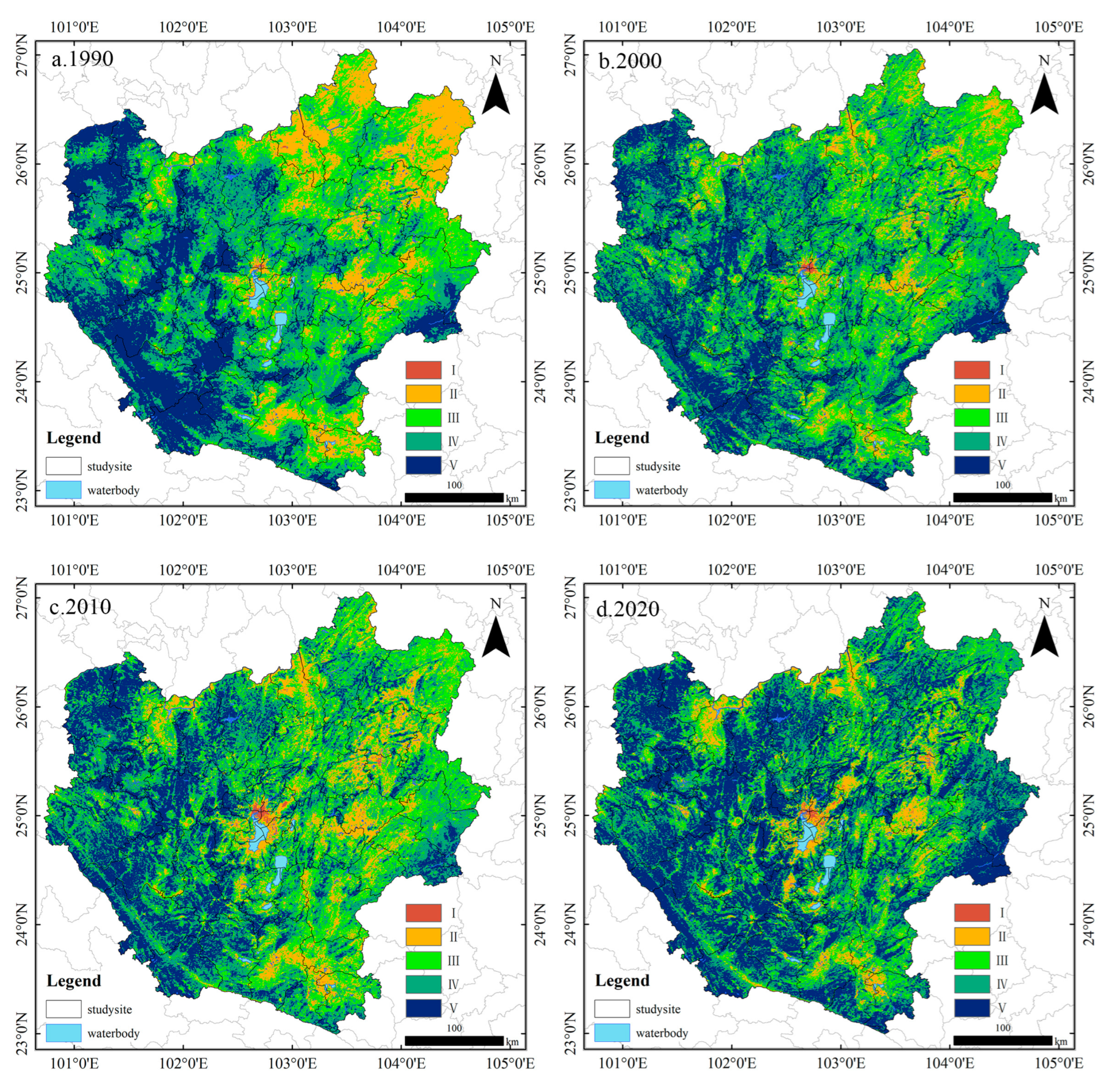
3.1. Spatial and Temporal Changes in FVC

Figure 4 shows the spatial distribution of FVC in CYUA from 1990 to 2020. Research indicated that the highest vegetation level was in the southwest of the study area, while the lower vegetation level was in the east and water body. The FVC change results of CYUA showed a gradual increase from north to south and east to west. Most areas have middle–high or high vegetation coverage and good ecological environment quality. Until 2020, the study area consistently had high vegetation coverage along the Ailao Mountains in the southwest, the northwest of Chuxiong, and Luoping and Shizong in the southeast of Qujing. In addition to water bodies and urban core areas, low-vegetation-coverage areas include Mengzi, Kaiyuan, and Jianshui in Honghe Prefecture in the south and Yuanmou and Yongren in the north of Chuxiong. The vegetation coverage in most areas of Qujing in the east has improved; however, Huize and Luliang still have low vegetation coverage levels. According to statistical analysis (Figure 4d), from 1990 to 2010, the highest proportion was Level IV (32.12%, 37.68%, 33.60%). In 2020, the highest proportion was Level V (39.92%). According to the data, over 55% of the total area falls under middle–high and high coverage (Level IV and V), which suggests robust vegetation growth and superior-quality green space.
The spatial transformation pattern of FVC levels in CYUA during different periods is shown in Figure 5. During 1990–2000, the total increase area (23.17%) was greater than the decrease area (10.57%). The increasing trend mainly occurred in Xuanwei, Huize, Dongchuan, and Fuyuan in the northeast and Mengzi in the south (Figure 5a,d). From 2000 to 2010, the overall decrease area was 7.19% greater than the increase area, and the decreasing trend (21.33%) was widely distributed spatially. Still, it was relatively concentrated in the Mile, Kaiyuan, and Ai’lao Mountains in the southwest (Figure 5b,d). From 2010 to 2020, the area increased significantly (34.77%), and the spatial distribution accounted for over half. From 1990 to 2020, the proportion of Level I gradually increased, and the area proportion of Level II fluctuated and decreased; Level III first increased and then reduced, and finally dropped by nearly 10%. Level IV conversions were the most active, peaking in 2000 (37.68%). By 2020, the proportion of Level V was the greatest (39.9%), mainly concentrated in Fuyuan, Luoping, Shizong, Luxi, and Mile in the east (Figure 5c,d).

3.2. Variation Trends Analysis of FVC

The significance judgment of the β value of the Theil–Sen estimator and the Z value of the Mann–Kendall test were used to obtain the spatial change trend distribution map of FVC in the CYAU from 1990 to 2020 (Figure 6). The different value ranges were set to represent areas with change trend characteristics, as shown in Table 4. Based on Figure 6 and Table 4, the main trends of FVC in the CYUA were divided into five categories: significant improvement, improvement, stable, slight degradation, and severe degradation. The improved vegetation cover areas (26.99%) were much more extensive than degraded ones (1.71%). Significant improvement (a 22.49% coverage) has been observed in the eastern karst landform and northern alpine meadow areas encompassing Xuanwei, Huize, Fuyuan, Xundian, Dongchuan and Chuxiong, Yao’an, Mouding, as shown in Figure 6d,e. Conversely, areas of severe degradation (1.56%) were predominantly located in the urban impervious regions of Guandu, Songming, Yiliang, Jinning, Hongta, Jiangchuan, Tonghai (in the center, Figure 6a), Qilin and Luliang (in the east, Figure 6b), and Mengzi (in the south, Figure 6c). The remaining vast areas (75.95%) have either remained stable or experienced minor changes. Urban expansion has led to a significant reduction in vegetation coverage around areas that were already severely degraded. However, afforestation and “Pearl River Source” ecological restoration projects in the Northeast have successfully improved the vegetation coverage.

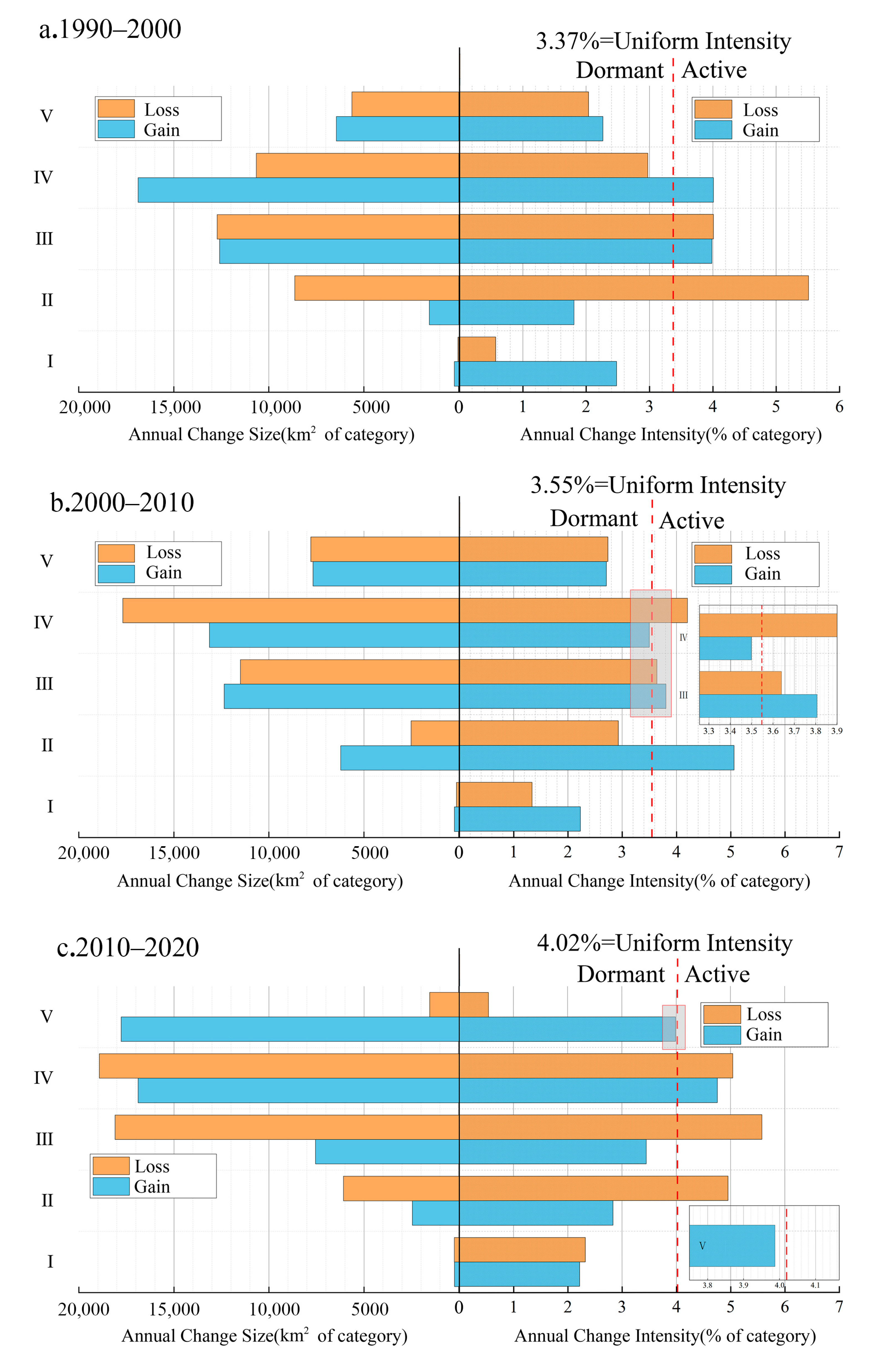
3.3. FVC Change at Time Interval, Category, and Transition Level

The results at the time level are shown in Figure 7. The average annual intensity of change in vegetation cover in the CYUA showed a continuously increasing trend. The change rate intensity from 2010 to 2020 is 4.02%/a > 3.65%/a (the uniform intensity). The annual rate of change for FVC during this time interval was the fastest, with the largest actual size of changes (left side of Figure 7).
The results of the category level are shown in Figure 8. In Figure 8a, during 1990–2000, Level IV increased the largest size, and at the same time, the gain intensity of Level IV was very active. The gain/loss intensities in Level III were relatively active, and the intensity of loss in Level II was the highest during this time period. In Figure 8b, the size of the increase and decrease in Level III were almost the same, but the gain intensity was greater than the loss intensity. Level IV has the largest reduction area and the highest loss intensity. Level II has the highest loss intensity. In Figure 8c, the area of severe reduction in Level III corresponds to the most active loss intensity, which is much larger than the uniform intensity. Level IV’s size of increase/decrease was huge, and the gain/loss intensity of that level was also very active. Level II showed an area reduced by a small amount, but its loss intensity was active.
The intensity changes in the III and IV levels were the most active during the three intervals. The left side of Figure 8 shows that the total of areas change of Level III during the three time intervals were 25,305.9 km2, 23,848.6 km2, and 25,639.4 km2. In the first two intervals, the annual gross gains and losses exceeded the uniform intensity. After 2010, the loss intensity became more active. Moreover, Level IV occupied the largest total change area at all time points, accounting for 36.5%, 38.9%, and 39.8%. Finally, the gain and loss bar extended to the right of the uniform line in the third time interval. Alongside Levels III and IV, we found the gains and losses bar of Level II played a major role. Level V remained balanced and stationary in the first two intervals, then in the third interval increased quickly, but the gains still did not extend to the uniform line (Figure 8c).
Prior to 2000, heightened agricultural endeavors aiming to augment food production led to a substantial reduction in low vegetation coverage. In contrast, measures to safeguard forests were initiated after 2000, ushering in a dynamic shift towards middle-to-high vegetation coverage. Furthermore, following 2010, the conversion intensity of areas characterized by middle–high to high vegetation coverage experienced an increase, primarily attributable to the implementation of policies safeguarding cultivated land and the environment.
Table 5 displays the various FVC transition intensities for each time interval. It is clear that the transitions at Level IV were inversely changed twice during the three time intervals, which meant that the transfer-from level and transfer-to level changed each other. So, Figure 9 reports the transition at Level IV. From 1990 to 2000, the target for the transition out of Level III was Level IV, with the rate reaching 3.46%. Meanwhile, the transition rate to Level V (2.17%) also exceeded the uniform intensity, presenting a tendency towards low to high vegetation coverage (Figure 9a). The interval 2000–2010 shows Level IV was the target for transitioning away from high vegetation levels (Figure 9b), with some vegetation degradation. In 2010–2020, Level IV underwent a transition similar to that of 1990–2000 (Figure 9c), with the actual gain size of Level V being 14.54%, much larger than that of 1990–2000.

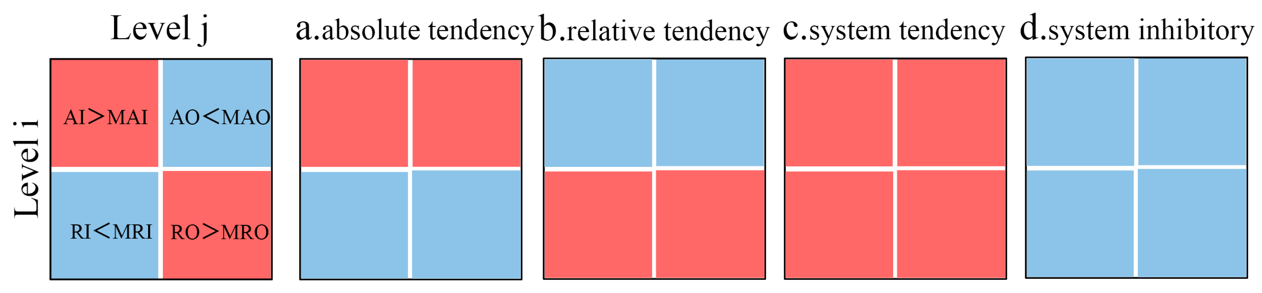
3.4. Transitions Level Change Tendency of FVC

The intensity map further analyzes the characteristics of FVC conversions in different time intervals, as shown in Figure 10.
From 1990 to 2000, the system’s tendency included Level II to Level III, Level III to Level IV, and Level IV to Level V. The actual intensity and relative intensity were larger than the mean intensity. The absolute tendency included Level IV to Level III, which showed that AIIV–III was greater than MAIIV–III and AOIV–III was greater than MAOIV–III, but RIIV–III was less than RAIIV–III and ROIV–III was less than RAOIV–III. The transitions in system tendency are all located on the upper right, indicating that the shift from a low to high level is dominant. At the same time, the actual intensity from Level IV to Level III is also powerful. From 2000 to 2010, the system tendency includes Level III to Level II, Level IV to Level III, Level V to Level IV, and Level IV to Level V. Some 75% of the system tendency occurs in the lower left, and the shift from a high level to low level became dominant. From 2010 to 2020, the system tendency type was the same as the first interval.
At the first time interval, there was an absolute tendency from Level IV to Level III, but a system tendency from Level III to Level IV and from Level IV to Level V; consequently, by the end of this period, the actual area size of Level IV had increased by 5.56% (as shown in Figure 5d). During the third time interval, Level III to Level IV and Level IV to Level V were all the system tendencies; the absolute intensity of AIV–IV from Level V to Level IV dropped significantly, and is smaller than MAIV–IV. This was no longer the system tendency at the previous time interval (Figure 10b,c). At the end of this period, Level V had the largest actual area size (39.92%, as shown in Figure 5d).

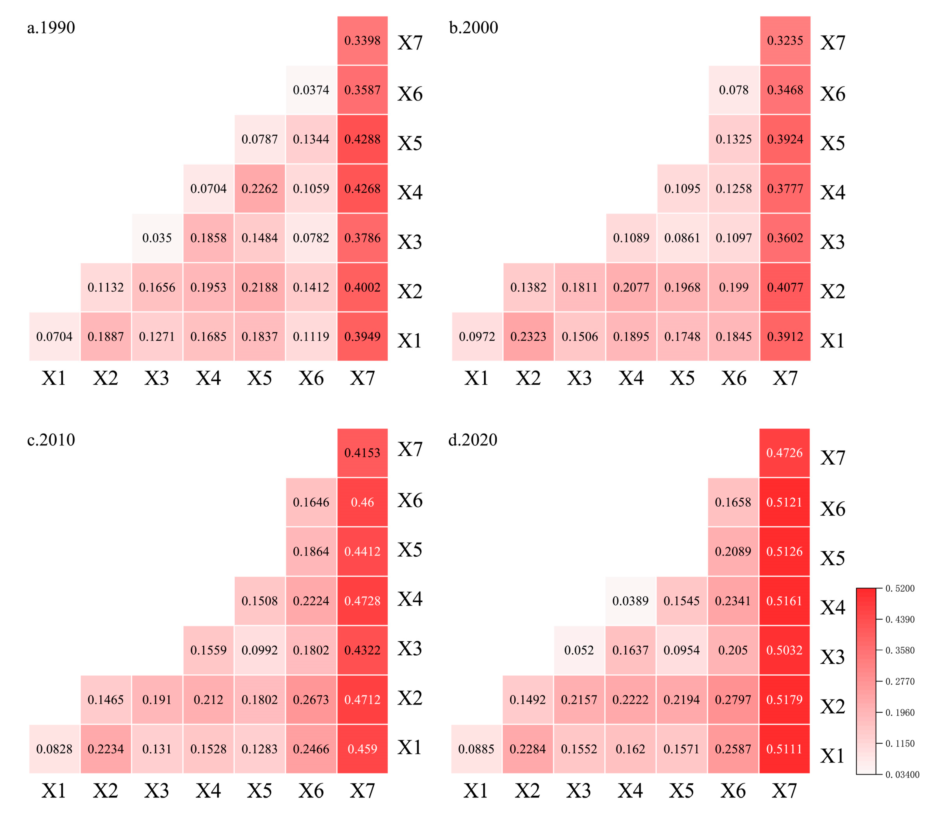
3.5. Contributions of the Climate Change and Human Activity Factors to FVC Changes

Figure 11 and Figure 12 display the outcomes of factor detection and interaction detection.
Based on Figure 11, the most noteworthy impact on spatiotemporal changes in the green space vegetation coverage of the CYUA is that of land cover (X7, q = 0.4726, p < 0.001). This factor has a significantly greater influence than others, and displays a positive trend. Additionally, nighttime lighting has a considerable impact (q = 0.1658, p < 0.001), with an explanatory power of over 16%, which is double the impact from 1990. Topographical factors, including aspect and slope, remain stable, with q values of 0.0885 (p < 0.001) and 0.1491 (p < 0.001), respectively. Among these, slope has a more significant influence. In this study, the meteorological factors of mean annual precipitation and mean annual temperature have a less than 10% explanatory power, indicating their limited influence. Overall, the impact of human factors has increased in significance over time. The results of aspect, slope, and elevation show a gradual increasing trend, while the impact of meteorological factors remains relatively stable.
The spatiotemporal difference of FVC in CYUA is the synergistic effect of multiple factors, which is more significant than that of a single factor. The interaction between any two factors is a complex and nonlinear combination of enhancement, and the interaction of land cover with any other factor creates the most synergistic effect. Strong interaction factors from 1990 to 2000 are slope∩mean annual temperature (q = 0.219), mean annual precipitation∩mean annual temperature (q = 0.226), aspect∩slope (q = 0.232), and slope∩mean annual precipitation (q = 0.208). From 2000 to 2020, nighttime lights–slope (q = 0.280) was the strongest factor, followed by nighttime lights∩aspect (q = 0.259), nighttime lights∩elevation (q = 0.205), nighttime lights∩mean annual precipitation (q = 0.234), and nighttime lights∩mean annual temperature (q = 0.209). This further indicates that landcover, nighttime lights, and slope are the key factors influencing FVC.

4. Discussion

4.1. Trends in the Patterns of FVC

This study effectively estimates spatial changes in FVC distribution in the central Yunnan urban agglomeration from 1990 to 2020 using the remote sensing index NDVI and the dimidiate pixel model. The examination of the spatial pattern was conducted through intensity analysis, whereas the investigation of the temporal trend was undertaken utilizing a linear model. The findings indicated that there was a gradual increase in the vegetative cover across the region, which was consistent with findings from previous studies, including global [14,32], national [60], and regional [25,61,62] scales, with a significant concentration of vegetation resources in the mountainous terrain. Urban areas are experiencing vegetation degradation, which has been confirmed multiple times [31,63].
We specifically focus on analyzing the areas with the highest level of urbanization in Yunnan Province over a longer period, which accurately reflects the dynamic characteristics of green space vegetation coverage in rapidly developing areas in which populations are gathering. Therefore, our research has identified that changes occur between middle–high to high vegetation coverage. We have also observed that the transformation of low vegetation cover primarily occurred in the northeastern regions, such as Xuanwei, Huize, and Xundian, from 1990 to 2000.
Over the past decade, the highest level of vegetation coverage has rapidly increased, predominantly in Xuanwei, Huize, and Dongchuan, as well as in Shizong, Fuyuan, and Luxi. In 2000, Zhanyi and Xuanwei established the Pearl River Source Nature Reserve to restore forests, water conservation, and the entire ecosystem. Since 2012, the eastern region has consistently expanded afforestation areas and implemented other ecological management projects such as rocky desertification control and soil erosion detection [64]. As a result, the expansion of forests and the mitigation of rocky desertification may have significantly contributed to improvements in ecological quality and the increase in FVC, as shown in Figure 4d and Figure 5c. Since 1990 to 2020, the vegetation coverage in the urban core area has decreased, indicating the impact of urbanization and human activities.

4.2. Changes in the Intensity of FVC

Intensity analysis is generally used for land use changes and is divided into three levels, further supplementing the original matrix analysis [65]. Some studies have applied this method to changes in vegetation coverage and found that it has good adaptability to vegetation coverage with different categories [29]. However, the intensity analysis needs a more straightforward description of the actual conversion sizes [56]. We introduced the intensity map method to compare the actual and relative intensity of FVC levels and draw intensity maps to analyze the tendency/inhibition further.
Based on the findings, it is evident that the coverage area of middle–high and high vegetation has been consistently expanding, as reflected in Figure 4 and Figure 5. Additionally, the rate of change from 2010 to 2020 has been the highest, as shown in Figure 7. While middle coverage played a significant role in the first time interval, middle–high and high coverage became more prominent in subsequent intervals, as depicted in Figure 8, Figure 9 and Figure 10. The proportion of forests in the CYUA is the highest (more than 50%). At the same time, the study site is also the most artificial afforested area in the province. Qujing has the largest artificial afforestation area at 31%, followed by Honghe Prefecture, at 27%. Yunnan has consistently prioritized the sustainable development of forests and implemented numerous management measures. The rapid increase in middle–high and high coverage is a testament to the effectiveness of forestry development in the past decade, as evidenced by Figure 4d, Figure 5c and Figure 13.

4.3. Differences in the Response of FVC Changes to Impact Factors

The CYUA has a mild climate, but in terms of precipitation, it is one of the most deficient areas in the province. The eastern part is a typical karst landform area, which is accompanied by rocky desertification. Kunming, Qujing, Yuxi, and Chuxiong have large populations, accounting for more than 40% of the entire province. Based on the characteristics of the study area, we selected influencing factors, and the results further proved the synergistic effect of natural and human factors.

4.3.1. Meteorological Factors

Temperature affects the transpiration of vegetation, while precipitation is the primary source of moisture. FVC changes stably responded to mean annual temperature and precipitation (taking 2020 as an example, as shown in Figure 14).
Recent studies have suggested that Yunnan Province is currently experiencing a warm and dry climate [66]. Additionally, research finds a positive correlation between mean annual precipitation and temperature with vegetation coverage in the CYUA, indicating that higher levels of precipitation and temperature can lead to more robust vegetation growth [67,68]. However, our study also notes that meteorological factors have a slightly weaker explanatory power when compared to topographic and human factors, possibly due to the type of vegetation cover and average altitude in the area. Research showed that the vegetation cover pattern of cultivated land at around 2000 m was mainly influenced by the slope of total primary productivity rather than meteorological factors [69,70], similar to the situation in eastern grain-producing regions. In the face of climate warming and the frequent occurrence of local disasters [71,72], moderate artificial intervention can alleviate the vulnerability and sensitivity of the region, making it increasingly dependent on the regulatory role of water conservancy projects.

4.3.2. Topographical Factors

Slope mattered more than aspect or elevation. Although over 90% of the region is mountainous, with elevations ranging from 127 m to over 4281 m, not all slopes are created equal. Plateau lakes and farmland, with slopes between 0° and 3°, account for only 4.56% of the region. In contrast, steeper areas, with slopes ranging from 24° to 81°, make up a significant 34.54% of the region, making vegetation coverage changes more challenging. Research indicated that slopes between 3° and 24° were optimal for vegetation survival and growth. However, as the slope becomes steeper and the terrain more complex, soil erosion becomes a more critical issue [73]. Slope affects the vertical distribution of water and heat conditions for vegetation survival, leading to heterogeneity in the topographic conditions of FVC in CYUA.

4.3.3. Human Factors

In recent years, human activities have had a significant impact on the environment, particularly in relation to economic activities and land use [74]. In 2008, researchers introduced a new perspective by utilizing nighttime light data to study economic development [75,76]. Since then, these data have been employed to investigate the effects of human activities on the environment, urban areas [77], climate change [78], and ecosystems [79]. In our exploration of the impact of human activity on vegetation coverage, we have opted to use nighttime light data as a measure.
Figure 15 illustrates that since 1993, the built-up area of the CYUA has continued to grow, and this is also the area shown in Figure 6, where vegetation coverage has significantly declined. Nighttime light has a strong explanatory influence on the FVC of the CYUA, as observed in Figure 11 and Figure 12 (qmax = 0.1658, sig. < 0.001), which confirms the accuracy of nighttime light data in characterizing human activities.
For this study, we reclassified the land cover into nine types: rainfed cropland (1), herbaceous cover (2), irrigated cropland (3), evergreen broadleaved forest (4), deciduous broadleaved forest (5), evergreen needle-leaved forest (6), shrubland (7), grassland (8) and other types (9). As shown in Figure 16, forest resources (evergreen broadleaved forest, deciduous broadleaved forest, evergreen needle-leaved forest, and shrubland) here are abundant, with a proportion of over 50%. It is a fact that forests have a much larger leaf area compared to other types of vegetation, which also confirms the distribution of high FVC levels in the study area (Figure 4). Forests are essential to the environment as they play a crucial role in regulating climate and providing habitats for countless species. In particular, the sharp increase in evergreen broad-leaved forest corresponded to the most actively transformed middle–high and high FVC levels among the three time intervals (Table 5 and Figure 9). Combined with ecological management measures such as closing hills for afforestation, returning farmland to forests, and artificial afforestation, the Pearl River’s ecological management and the frequency and intensity of mutual transfer of land cover types have increased, which enhances the sizes forests and grassland areas and optimizes the green space’s structure (Figure 4 and Figure 5).

4.3.4. Factors Interaction Effect

We found that the interaction between driving factors is more significant than a single factor, consistent with many studies [80,81,82,83]. Although meteorological and topographic factors have a relatively weak overall influence on vegetation changes (as shown in Figure 11), their explanatory power increased significantly after 2010 due to a non-linear enhancement effect between land cover and each other factor (as depicted in Figure 12). Specifically, the interactions between land cover and other factors surpassed 0.30 (as shown in Figure 12). In order to promote higher-quality development in the CYUA, it is essential to strengthen greening construction. However, due to the general water shortage in these urban agglomerations, the slope factor plays a crucial role in controlling temperature and precipitation gradient distribution. Therefore, it is imperative to focus on land and water conservation under the influence of slope. Nighttime lighting has played a nonlinear enhancement role since 2010. Urban economic activities have increased, and the scope of construction has continued to expand. “Towns moving up the mountain” have revitalized surrounding mountain resources and affected vegetation coverage.

5. Conclusions

Over the past three decades, the spatial distribution of vegetation cover in the CYUA has shown the following trends.
(1)
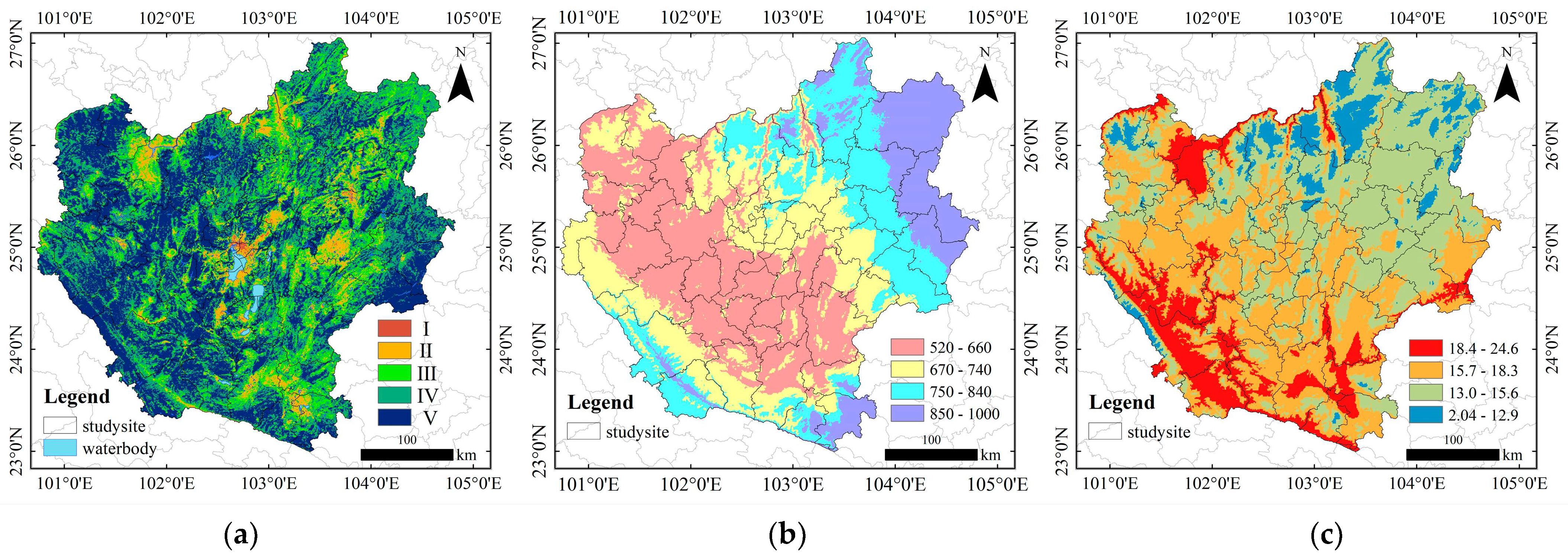
Vegetation cover gradually decreased from south to north and from west to east.
(2)
As of 2020, the proportion of vegetation coverage levels is as follows: high vegetation coverage (Level V) > middle–high vegetation coverage (Level IV) > middle vegetation coverage (Level III) > low vegetation coverage (Level I/Level II).
According to our trend analysis,
(3)
Overall, there is a 26.99% area of improvement and only a 1.71% area of degradation.
(4)
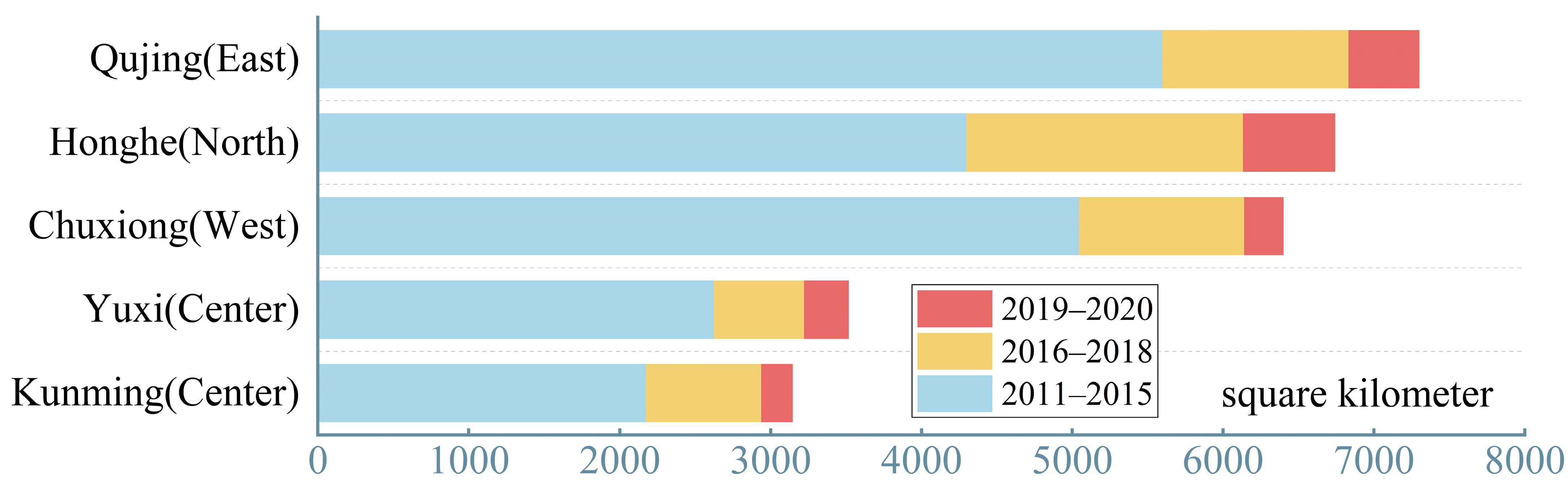
Specifically, the areas with significant improvement in vegetation coverage were the eastern karst landform area and plateau meadow area (22.49%). In comparison, the areas with severe degradation were distributed in the central and eastern core areas of human activity (1.56%).
According to our intensity analysis,
(5)
The intensity of the time intervals increased by 1.19 times. At the category level, the most active gain/loss was in middle and middle–high vegetation coverage. At the transition level, the middle–high vegetation coverage changed significantly, being associated with forest protection and artificial afforestation in the CYUA.
According to our analysis of driving factors,
(6)
The factors that had an influence greater than 10% from 1990 to 2020 were land cover > slope before 2010; after 2010, the factors with the greatest influence were land cover > nighttime light > slope.
(7)
The most significant synergy between land cover and other factors is greater than 0.30. Land cover change is further accelerated due to increased human activities and urbanization.
The rapid growth of the urban center of the CYUA has led to several environmental concerns, particularly with regard to the depletion of natural green spaces and vegetation cover. This phenomenon poses a threat to the aesthetic appeal of the city, and has far-reaching ecological consequences such as increased soil erosion, heightened air pollution levels, and loss of biodiversity. As such, it is imperative to implement strategic measures to curb these negative effects and preserve the surrounding regions’ inherent natural beauty.

Author Contributions

Conceptualization, Y.L. and Y.S.; methodology, Y.L., X.C. and Y.S.; software, Y.L.; validation, Y.L., L.H. and J.Z.; formal analysis, Y.L. and Y.S.; investigation, Y.L., L.H. and J.Z.; resources, Y.L.; writing—original draft preparation, Y.L.; writing—review and editing, Y.L.; visualization, Y.L., L.H. and J.Z.; supervision, Y.S.; project administration, Y.S.; funding acquisition, Y.S. All authors have read and agreed to the published version of the manuscript.

Funding

This research was funded by Yunnan Province High-level Talents Training Support Program, grant number YNWR-CYJS-2020-022; and the Scientific and Yunnan University Minority Gardens, and beautiful countryside Science and Technology Innovation Team.

Institutional Review Board Statement

Not applicable.

Informed Consent Statement

Not applicable.

Data Availability Statement

Data are contained within the article.

Acknowledgments

The authors acknowledge data support from the Loess Plateau SubCenter, the National Earth System Science Data Center, and National Science and Technology Infrastructure of China. (http://loess.geodata.cn) (accessed on 20 November 2023).

Conflicts of Interest

The authors declare no conflicts of interest.

References

  1. World Cities Report 2022: Envisaging the Future of Cities, the United Nations Human Settlements Programme. Available online: https://unhabitat.org/wcr/ (accessed on 20 November 2023).
  2. Najihah, N.A.M.; Corstanje, R.; Harris, J.A.; Brewer, T. Impact of rapid urban expansion on greenspace structure. Ecol. Indic. 2017, 81, 274–284. [Google Scholar] [CrossRef]
  3. Wang, J.; Zhang, Y.; Zhang, X.; Song, M.; Ye, J. The spatio-temporal trends of urban green space and its interactions with urban growth: Evidence from the Yangtze River Delta region, China. Land Use Policy 2023, 128, 106598. [Google Scholar] [CrossRef]
  4. Yin, H.W.; Kong, F.H.; Zong, Y.G. Accessibility and Equity Assessment on Urban Green Space. Acta Ecol. Sin. 2008, 28, 3375–3383. Available online: https://kns.cnki.net/kcms2/article/abstract?v=TzO8JwpG6ugQJ4d6aYgKBriI7-x8Gb5qDx1NP-WXKVYe0Wf3qELif_BlTnPkBbenhAH6bd1LD1dkPQsZAhdT-4TP8Hisvq8M313SxYZQhM5FQAnXY4KUG6nZqb3QpiQ-&uniplatform=NZKPT&language=CHS (accessed on 20 November 2023).
  5. Zheng, L.Y.; Pu, H.X.; Jiang, Z.P. Spatial satisfaction of urban parks based on the visible green index. J. Nanjing For. Univ. (Nat. Sci. Ed.) 2020, 44, 199–204. [Google Scholar] [CrossRef]
  6. Wu, S.; Wang, D.; Yan, Z.; Wang, X.; Han, J. Spatiotemporal dynamics of urban green space in Changchun: Changes, transformations, landscape patterns, and drivers. Ecol. Indic. 2023, 147, 109958. [Google Scholar] [CrossRef]
  7. Matsa, M.; Mupepi, O.; Musasa, T. Spatio-temporal analysis of urban expansion in Gweru city, Zimbabwe between 1990 and 2020. Environ. Chall. 2021, 4, 100141. [Google Scholar] [CrossRef]
  8. Paudel, S.; States, S.L. Urban green spaces and sustainability: Exploring the ecosystem services and disservices of grassy lawns versus floral meadows. Urban For. Urban Green 2023, 84, 127932. [Google Scholar] [CrossRef]
  9. Qin, W.; Zhu, Q.k.; Zhang, X.x.; Li, W.h.; Fang, B. Review of vegetation covering and its measuring and calculating method. J. Northwest Sci-Tech Univ. Agric. For. (Nat. Sci. Ed.) 2006, 34, 163–168. [Google Scholar]
  10. Ren, Y.; Zhang, F.; Zhao, C.; Cheng, Z. Attribution of climate change and human activities to vegetation NDVI in Jilin Province, China during 1998–2020. Ecol. Indic. 2023, 153, 110415. [Google Scholar] [CrossRef]
  11. Jiapaer, G.; Chen, X.; Bao, A. A comparison of methods for estimating fractional vegetation cover in arid regions. Agric. For. Meteorol. 2011, 151, 1698–1710. [Google Scholar] [CrossRef]
  12. Carlson, T.N.; Ripley, D.A. On the relation between NDVI, fractional vegetation cover, and leaf area index. Remote Sens. Environ. 1997, 62, 241–252. [Google Scholar] [CrossRef]
  13. Chu, D.; Chu, D. Fractional vegetation cover. In Remote Sensing of Land Use and Land Cover in Mountain Region; Springer: Berlin/Heidelberg, Germany, 2020; pp. 195–207. [Google Scholar] [CrossRef]
  14. Wu, D.; Wu, H.; Zhao, X.; Zhou, T.; Tang, B.; Zhao, W.; Jia, K. Evaluation of Spatiotemporal Variations of Global Fractional Vegetation Cover Based on GIMMS NDVI Data from 1982 to 2011. Remote Sens. 2014, 6, 4217–4239. [Google Scholar] [CrossRef]
  15. Gutman, G.; Ignatov, A. The derivation of the green vegetation fraction from NOAA/AVHRR data for use in numerical weather prediction models. Int. J. Remote Sens. 1998, 19, 1533–1543. [Google Scholar] [CrossRef]
  16. Amiri, R.; Weng, Q.; Alimohammadi, A.; Alavipanah, S.K. Spatial-temporal dynamics of land surface temperature in relation to fractional vegetation cover and land use/cover in the Tabriz urban area, Iran. Remote Sens. Environ. 2009, 113, 2606–2617. [Google Scholar] [CrossRef]
  17. Song, W.; Mu, X.; Ruan, G.; Gao, Z.; Li, L.; Yan, G.; Yan, G. Estimating fractional vegetation cover and the vegetation index of bare soil and highly dense vegetation with a physically based method. Int. J. Appl. Earth Obs. Geoinf. 2017, 58, 168–176. [Google Scholar] [CrossRef]
  18. Ren, H.; Wen, Z.; Liu, Y.; Lin, Z.; Han, P.; Shi, H.; Wang, Z.; Su, T. Vegetation response to changes in climate across different climate zones in China. Ecol. Indic. 2023, 155, 110932. [Google Scholar] [CrossRef]
  19. Liu, H.Q.; Huete, A. A feedback-based modification of the NDVI to minimize canopy background and atmospheric noise. IEEE Trans. Geosci. Remote Sens. 1995, 33, 457–465. [Google Scholar] [CrossRef]
  20. Sun, H.; Wang, C.; Niu, Z. Analysis of the vegetation cover change and the relationship between NDVI and environmental factors by using NOAA time series data. J. Remote Sens. 1998, 2, 210–216. [Google Scholar] [CrossRef]
  21. Gao, L.; Wang, X.; Johnson, B.A.; Tian, Q.; Wang, Y.; Verrelst, J.; Mu, X.; Gu, X. Remote sensing algorithms for estimation of fractional vegetation cover using pure vegetation index values: A review. ISPRS J. Photogramm. Remote Sens. 2020, 159, 364–377. [Google Scholar] [CrossRef]
  22. Wittich, K.P.; Hansing, O. Area-averaged vegetative cover fraction estimated from satellite data. Int. J. Biometeorol. 1995, 38, 209–215. [Google Scholar] [CrossRef]
  23. Zhang, W.; Randall, M.; Jensen, M.B.; Brandt, M.; Wang, Q.; Fensholt, R. Socio-economic and climatic changes lead to contrasting global urban vegetation trends. Glob. Environ. Chang. 2021, 71, 101883. [Google Scholar] [CrossRef]
  24. Jiang, S.; Zhang, Z.; Wang, W.; Du, W.; Jin, Q. Dynamic variation rules of vegetation cover in Jiangsu Province and its response to climate change. J. Nanjing For. Univ. (Nat. Sci. Ed.) 2016, 40, 74–80. [Google Scholar] [CrossRef]
  25. Liu, C.; Zhang, X.; Wang, T.; Chen, G.; Zhu, K.; Wang, Q.; Wang, J. Detection of vegetation coverage changes in the Yellow River Basin from 2003 to 2020. Ecol. Indic. 2022, 138, 108818. [Google Scholar] [CrossRef]
  26. Bille, R.A.; Jensen, K.E.; Buitenwerf, R. Global patterns in urban green space are strongly linked to human development and population density. Urban For. Urban Green. 2023, 86, 127980. [Google Scholar] [CrossRef]
  27. Zheng, B.; Myint, S.W.; Fan, C. Spatial configuration of anthropogenic land cover impacts on urban warming. Landsc. Urban Plan. 2014, 130, 104–111. [Google Scholar] [CrossRef]
  28. Ma, B.; Wang, S.; Mupenzi, C.; Li, H.; Ma, J.; Li, Z. Quantitative Contributions of Climate Change and Human Activities to Vegetation Changes in the Upper White Nile River. Remote Sens. 2021, 13, 3648. [Google Scholar] [CrossRef]
  29. Tong, S.; Zhang, J.; Ha, S.; Lai, Q.; Ma, Q. Dynamics of Fractional Vegetation Coverage and Its Relationship with Climate and Human Activities in Inner Mongolia, China. Remote Sens. 2016, 8, 776. [Google Scholar] [CrossRef]
  30. Wei, X.; Wang, S.; Wang, Y. Spatial and temporal change of fractional vegetation cover in North-western China from 2000 to 2010. Geol. J. 2018, 53, 427–434. [Google Scholar] [CrossRef]
  31. Mao, P.; Zhang, J.; Li, M.; Liu, Y.; Wang, X.; Yan, R.; Shen, B.; Zhang, X.; Shen, J.; Zhu, X.; et al. Spatial and temporal variations in fractional vegetation cover and its driving factors in the Hulun Lake region. Ecol. Indic. 2022, 135, 108490. [Google Scholar] [CrossRef]
  32. Jiang, L.; Jiapaer, G.; Bao, A.; Guo, H.; Ndayisaba, F. Vegetation dynamics and responses to climate change and human activities in Central Asia. Sci. Total Environ. 2017, 599–600, 967–980. [Google Scholar] [CrossRef]
  33. de Beurs, K.M.; Henebry, G.M.; Owsley, B.C.; Sokolik, I. Using multiple remote sensing perspectives to identify and attribute land surface dynamics in Central Asia 2001–2013. Remote Sens. Environ. 2015, 170, 48–61. [Google Scholar] [CrossRef]
  34. Li, Y.; Zheng, Z.; Qin, Y.; Rong, P. Relative contributions of natural and man-made factors to vegetation cover change of environmentally sensitive and vulnerable areas of China. J. Clean. Prod. 2021, 321, 128917. [Google Scholar] [CrossRef]
  35. Zhang, Y.; Ye, A. Quantitatively distinguishing the impact of climate change and human activities on vegetation in mainland China with the improved residual method. GISci. Remote Sens. 2021, 58, 235–260. [Google Scholar] [CrossRef]
  36. Wang, J.F.; Zhang, T.L.; Fu, B.J. A measure of spatial stratified heterogeneity. Ecol. Indic. 2016, 67, 250–256. [Google Scholar] [CrossRef]
  37. Fang, C. Progress and the future direction of research into urban agglomeration in China. Acta Geogr. Sin. 2014, 69, 1130–1144. [Google Scholar] [CrossRef]
  38. The Government Work Report of Yunnan Province. 2023. Available online: https://www.yn.gov.cn/zwgk/zfxxgk/zfgzbg/202302/t20230207_254669.html (accessed on 20 November 2023).
  39. Wang, Y.; Lu, H. Driving force of vegetation cover change in Yunnan province of China from 2001 to 2018. Mt. Res. 2022, 40, 531–541. [Google Scholar] [CrossRef]
  40. Wang, J.F.; Li, X.H.; Christakos, G.; Liao, Y.L.; Zhang, T.; Gu, X.; Zheng, X.Y. Geographical detectors-based health risk assessment and its application in the neural tube defects study of the Heshun region, China. Int. J. Geogr. Inf. Sci. 2010, 24, 107–127. [Google Scholar] [CrossRef]
  41. “Development Plan for Urban Agglomeration in Central Yunnan”, Yunnan Provincial People’s Government. Available online: https://www.yn.gov.cn/zwgk/zfxxgkpt/fdzdgknr/zcwj/zdgkwjyzf/202008/t20200826_209715.html (accessed on 20 November 2023).
  42. Liu, H.; Zhou, T.; Gou, P. NDVI Dataset of China and Average in 361 Cities (250 m, 1990–2020). Digit. J. Glob. Chang. Data Repos. 2023, 10. Available online: https://www.geodoi.ac.cn/edoi.aspx?DOI=10.3974/geodb.2023.04.06.V1 (accessed on 20 November 2023).
  43. Zhou, T.; Liu, H.; Gou, P.; Xu, N. Conflict or Coordination? Measuring the Relationships Between Urbanization and Vegetation Cover in China. Ecol. Indic. 2023, 147, 106941. [Google Scholar] [CrossRef]
  44. Peng, S.; Ding, Y.; Liu, W.; Li, Z. 1 km monthly temperature and precipitation dataset for China from 1901 to 2017. Earth Syst. Sci. Data 2019, 11, 1931–1946. [Google Scholar] [CrossRef]
  45. Loess Plateau SubCenter, National Earth System Science Data Center, National Science & Technology Infrastructure of China. Available online: http://loess.geodata.cn (accessed on 20 November 2023).
  46. Li, X.; Zhou, Y.; Zhao, M.; Zhao, X. Harmonization of DMSP and VIIRS nighttime light data from 1992–2018 at the global scale. 2020. Available online: https://figshare.com/articles/dataset/Harmonization_of_DMSP_and_VIIRS_nighttime_light_data_from_1992-2018_at_the_global_scale/9828827 (accessed on 20 November 2023). [CrossRef]
  47. Zhao, M.; Cheng, C.; Zhou, Y.; Li, X.; Shen, S.; Song, C. A global dataset of annual urban extents (1992–2020) from harmonized nighttime lights. Earth Syst. Sci. Data 2021, 14, 517–534. [Google Scholar] [CrossRef]
  48. Zhang, X.; Liu, L.; Chen, X.; Gao, Y.; Xie, S.; Mi, J. GLC_FCS30: Global land-cover product with fine classification system at 30 m using time-series Landsat imagery. Earth Syst. Sci. Data Discuss. 2021, 13, 2753–2776. [Google Scholar] [CrossRef]
  49. Zhang, X.; Liu, L.; Wu, C.; Chen, X.; Gao, Y.; Xie, S.; Zhang, B. Development of a global 30 m impervious surface map using multisource and multitemporal remote sensing datasets with the Google Earth Engine platform. Earth Syst. Sci. Data 2020, 12, 1625–1648. [Google Scholar] [CrossRef]
  50. Ministry of Ecology and Environment of the People’s Republic of China. Available online: https://www.mee.gov.cn/ (accessed on 20 November 2023).
  51. Tudor, C. Ozone pollution in London and Edinburgh: Spatiotemporal characteristics, trends, transport and the impact of COVID-19 control measures. Heliyon 2022, 8, e11384. [Google Scholar] [CrossRef]
  52. Bu, H.; Wulan, T.Y.; Siqin, C.K.T.; Han, S.M.; Gao, S.R.G.; Wu, X.Q. Response of vegetation fraction cover change to meteorological drought in Inner Mongolia from 1982 to 2099. J. Northwest For. Univ. 2023, 5, 1–9. [Google Scholar] [CrossRef]
  53. Wang, L.; Li, W.; Zheng, Y.; Zhang, X.; Yuan, F.; Wu, X. Water Deficit Caused by Land Use Changes and Its Implications on the Ecological Protection of the Endorheic Dalinor Lake Watershed in Inner Mongolia, China. Water 2023, 15, 2882. [Google Scholar] [CrossRef]
  54. Xu, T.; Wu, H. Spatiotemporal Analysis of Vegetation Cover in Relation to Its Driving Forces in Qinghai–Tibet Plateau. Forests 2023, 14, 1835. [Google Scholar] [CrossRef]
  55. Aldwaik, S.Z.; Pontius, R.G., Jr. Intensity analysis to unify measurements of size and stationarity of land changes by interval, category, and transition. Landsc. Urban Plan. 2012, 106, 103–114. [Google Scholar] [CrossRef]
  56. Li, S.C.; Gong, J.; Yang, J.X.; Chen, G.; Zhang, Z.; Zhang, M.Q. Characteristics of LUCC patterns of the Lanzhou-Xining urban agglomeration: Based on an intensity analysis framework. Resour. Sci. 2023, 45, 480–493. [Google Scholar] [CrossRef]
  57. Mu, B.; Zhao, X.; Zhao, J.; Liu, N.; Si, L.; Wang, Q.; Sun, N.; Sun, M.; Guo, Y.; Zhao, S. Quantitatively Assessing the Impact of Driving Factors on Vegetation Cover Change in China’s 32 Major Cities. Remote Sens. 2022, 14, 839. [Google Scholar] [CrossRef]
  58. Zheng, Y.; He, Y.; Zhou, Q.; Wang, H. Quantitative Evaluation of Urban Expansion using NPP-VIIRS Nighttime Light and Landsat Spectral Data. Sustain. Cities Soc. 2021, 76, 338. [Google Scholar] [CrossRef]
  59. Zhou, X.; Wen, H.; Zhang, Y.; Xu, J.; Zhang, W. Landslide susceptibility mapping using hybrid random forest with GeoDetector and RFE for factor optimization. Geosci. Front. 2021, 12, 101211. [Google Scholar] [CrossRef]
  60. Kong, Z.; Ling, H.; Deng, M.; Han, F.; Yan, J.; Deng, X.; Wang, Z.; Ma, Y.; Wang, W. Past and projected future patterns of fractional vegetation coverage in China. Sci. Total Environ. 2023, 902, 166133. [Google Scholar] [CrossRef] [PubMed]
  61. Yang, S.; Song, S.; Li, F.; Yu, M.; Yu, G.; Zhang, Q.; Cui, H.; Wang, R.; Wu, Y. Vegetation coverage changes driven by a combination of climate change and human activities in Ethiopia, 2003–2018. Ecol. Inform. 2022, 71, 101776. [Google Scholar] [CrossRef]
  62. Wang, Z.; Wang, Y.; Liu, Y.; Wang, F.; Deng, W.; Rao, P. Spatiotemporal characteristics and natural forces of grassland NDVI changes in Qilian Mountains from a sub-basin perspective. Ecol. Indic. 2023, 157, 111186. [Google Scholar] [CrossRef]
  63. Wang, Y.; Li, M. Annually Urban Fractional Vegetation Cover Dynamic Mapping in Hefei, China (1999–2018). Remote Sens. 2021, 13, 2126. [Google Scholar] [CrossRef]
  64. Li, W.; Wang, W.; Chen, J.; Zhang, Z. Assessing effects of the Returning Farmland to Forest Program on vegetation cover changes at multiple spatial scales: The case of northwest Yunnan, China. J. Environ. Manag. 2022, 304, 114303. [Google Scholar] [CrossRef] [PubMed]
  65. Mallinis, G.; Koutsias, N.; Arianoutsou, M. Monitoring land use/land cover transformations from 1945 to 2007 in two peri-urban mountainous areas of Athens metropolitan area, Greece. Sci. Total Environ. 2014, 490, 262–278. [Google Scholar] [CrossRef]
  66. Sun, H.; Wang, J.; Xiong, J.; Bian, J.; Jin, H.; Cheng, W.; Li, A. Vegetation change and its response to climate change in Yunnan Province, China. Adv. Meteorol. 2021, 2021, 8857589. [Google Scholar] [CrossRef]
  67. Shi, H.; Chen, J. Characteristics of climate change and its relationship with land use/cover change in Yunnan Province, China. Int. J. Climatol. 2018, 38, 2520–2537. [Google Scholar] [CrossRef]
  68. Hillman, A.L.; Yu, J.; Abbott, M.B.; Cooke, C.A.; Bain, D.J.; Steinman, B.A. Rapid environmental change during dynastic transitions in Yunnan Province, China. Quat. Sci. Rev. 2014, 98, 24–32. [Google Scholar] [CrossRef]
  69. Zhang, C.; He, H.; Mokhtar, A. The impact of climate change and human activity on spatiotemporal patterns of multiple cropping index in South West China. Sustainability 2019, 11, 5308. [Google Scholar] [CrossRef]
  70. Tao, J.; Zhu, J.; Zhang, Y.; Dong, J.; Zhang, X. Divergent effects of climate change on cropland ecosystem water use efficiency at different elevations in southwestern China. J. Geogr. Sci. 2022, 32, 1601–1614. [Google Scholar] [CrossRef]
  71. He, Y.; Zhou, C.; Ahmed, T. Vulnerability assessment of rural social-ecological system to climate change: A case study of Yunnan Province, China. Int. J. Clim. Chang. Strateg. Manag. 2021, 13, 162–180. [Google Scholar] [CrossRef]
  72. Sun, L.; Jaramillo, F.; Cai, Y.; Zhou, Y.; Shi, S.; Zhao, Y.; Gunnarson, B. Exploring the influence of reservoir impoundment on surrounding tree growth. Adv. Water Resour. 2021, 153, 103946. [Google Scholar] [CrossRef]
  73. Gu, Z.; Bai, Z.; Duan, X.; Ding, J.; Feng, D.; Shi, X.; Han, X. Quantitative effects of environmental factors on climatic yield in the mountainous area: A case study in Yunnan Province. Chin. J. Agrometeorol. 2015, 36, 497. Available online: https://zgnyqx.ieda.org.cn//EN/Y2015/V36/I04/497 (accessed on 20 November 2023).
  74. Fan, F.; Xiao, C.; Feng, Z.; Yang, Y. Impact of human and climate factors on vegetation changes in mainland Southeast Asia and Yunnan Province of China. J. Clean. Prod. 2023, 415, 137690. [Google Scholar] [CrossRef]
  75. Gibson, J.; Olivia, S.; Boe-Gibson, G. Night lights in economics: Sources and uses 1. J. Econ. Surv. 2020, 34, 955–980. [Google Scholar] [CrossRef]
  76. Levin, N.; Kyba, C.C.; Zhang, Q.; de Miguel, A.S.; Román, M.O.; Li, X.; Elvidge, C.D. Remote sensing of night lights: A review and an outlook for the future. Remote Sens. Environ. 2020, 237, 111443. [Google Scholar] [CrossRef]
  77. Dong, B.; Yang, Y.; You, S.; Zheng, Q.; Huang, L.; Zhu, C.; Tong, C.; Li, S.; Li, Y. Identifying and Classifying Shrinking Cities Using Long-Term Continuous Night-Time Light Time Series. Remote Sens. 2021, 13, 3142. [Google Scholar] [CrossRef]
  78. Cai, D.; Fraedrich, K.; Guan, Y.; Guo, S.; Zhang, C. Urbanization and climate change: Insights from eco-hydrological diagnostics. Sci. Total Environ. 2019, 647, 29–36. [Google Scholar] [CrossRef]
  79. Bennie, J.; Davies, T.W.; Cruse, D.; Bell, F. Artificial light at night alters grassland vegetation species composition and phenology. J. Appl. Ecol. 2017, 55, 442–450. [Google Scholar] [CrossRef]
  80. Liu, C.; Li, W.; Wang, W.; Zhou, H.; Liang, T.; Hou, F.; Xu, J.; Xue, P. Quantitative spatial analysis of vegetation dynamics and potential driving factors in a typical alpine region on the northeastern Tibetan Plateau using the Google Earth Engine. CATENA 2021, 206, 105500. [Google Scholar] [CrossRef]
  81. Zuo, Y.; Li, Y.; He, K.; Wen, Y. Temporal and spatial variation characteristics of vegetation coverage and quantitative analysis of its potential driving forces in the Qilian Mountains, China, 2000–2020. Ecol. Indic. 2022, 143, 109429. [Google Scholar] [CrossRef]
  82. Xu, X.; Jiang, H.; Guan, M.; Wang, L.; Huang, Y.; Jiang, Y.; Wang, A. Vegetation responses to extreme climatic indices in coastal China from 1986 to 2015. Sci. Total Environ. 2020, 744, 140784. [Google Scholar] [CrossRef]
  83. Zhang, S.; Zhou, Y.; Yu, Y.; Li, F.; Zhang, R.; Li, W. Using the Geodetector Method to Characterize the Spatiotemporal Dynamics of Vegetation and Its Interaction with Environmental Factors in the Qinba Mountains, China. Remote Sens. 2022, 14, 5794. [Google Scholar] [CrossRef]
Figure 1. Workflow of this study.
Sustainability 16 00661 g001
Figure 2. The location of the study site.
Sustainability 16 00661 g002
Figure 3. Intensity map unit from i level to j level. (a) absoute tendency; (b) relative tendency; (c) system tendency; (d) system inhibitory.
Sustainability 16 00661 g003
Figure 4. Spatial distribution of FVC level in each interval in CYUA (a) 1990; (b) 2000; (c) 2010; (d) 2020.
Sustainability 16 00661 g004
Figure 5. Spatial transfer distribution patterns of FVC from 1990 to 2020 in CYUA: (a) patterns from 1990 to 2000; (b) patterns from 2000 to 2010; (c) patterns from 2010 to 2020; (d) levels of distribution of FVC from 1990 to 2020.
Sustainability 16 00661 g005
Figure 6. Trends in FVC from 1990 to 2020 in the CYUA ((ac) are three areas of severe degradation, (d,e) are two areas of significant improvement).
Sustainability 16 00661 g006
Figure 7. Time intensity analysis for three intervals, 1990–2000, 2000–2010, and 2010–2020, in the CYUA.
Sustainability 16 00661 g007
Figure 8. Category intensity analysis for three time intervals in the CYUA: (a) from 1990 to 2000, (b) from 2000 to 2010, and (c) from 2010 to 2020.
Sustainability 16 00661 g008
Figure 9. Annual intensity of the Level IV transformation from other categories in the CYUA. (a) 1990–2000; (b) 2000–2010; (c) 2010–2020.
Sustainability 16 00661 g009
Figure 10. Intensity map results of FVC in CYUA. (a) map of 1990–2000; (b) map of 2000–2010; (c) map of 2010–2020.
Sustainability 16 00661 g010
Figure 11. Q statistic for single-factor detection results of FVC change from 1990 to 2020 in the CYUA.
Sustainability 16 00661 g011
Figure 12. Interaction detection results of factors influencing FVC change from 1990 to 2020 in the CYUA.(a) results of 1990; (b) results of 2000; (c) results of 2010; (d) results of 2020.
Sustainability 16 00661 g012
Figure 13. Total area of afforestation from 2011 to 2020 in the CYUA.
Sustainability 16 00661 g013
Figure 14. Spatial distribution of (a) vegetation coverage, (b) mean annual precipitation, and (c) mean annual temperature for 2020.
Sustainability 16 00661 g014
Figure 15. The relationship between urban built-up area squares and nightlight data from 1993 to 2020.
Sustainability 16 00661 g015
Figure 16. Land cover map from 1990–2020 in the CYUA.
Sustainability 16 00661 g016
Table 1. Study data and sources.
DataData AccuracyData SourcesData URL
Normalized difference vegetation index (NDVI) data [42,43]250 mGlobal Change Research Data Publishing and Repositoryhttps://www.geodoi.ac.cn/ (accessed on 20 November 2023)
DEM data30 mGeospatial data cloudhttps://www.gscloud.cn/ (accessed on 20 November 2023)
Annual average precipitation
data [44]
1000 mNational Earth System Science Data Center, National Science and Technology Infrastructure of Chinahttp://loess.geodata.cn (accessed on 20 November 2023)
Annual average temperature data [45]1000 mNational Earth System Science Data Center, National Science and Technology Infra-structure of Chinahttp://loess.geodata.cn (accessed on 20 November 2023)
Nighttime light data [46,47]1000 mA global dataset of annual urban extents (1992–2020) from harmonized nighttime lights. figshare.https://doi.org/10.6084/m9.figshare.9828827.v2 (accessed on 20 November 2023)
Land cover/use data [48,49]30 mBig Earth Data Science Engineering Programhttps://data.casearth.cn/ (accessed on 20 November 2023)
Afforestation data/Yearbook of Yunnan Provincial Bureau of Statisticshttp://stats.yn.gov.cn/ (accessed on 20 November 2023)
Table 2. The FVC classification.
CategoriesCategories NameLandscape Features
I LevelExtremely low coverage0 ≤ FVC ≤ 35%
No vegetation, water bodies, bare land, rock, residential areas, high rocky desertification
II LevelLow coverage35% < FVC ≤ 55%
Sparse vegetation, sparse grassland, built-up area, middle-level rocky desertification
III LevelMiddle coverage55% < FVC ≤ 65%
Middle-yield grassland, arable land, and green land in built-up areas
IV LevelMiddle–high coverage65% < FVC ≤ 75%
Higher-yield grassland, arable land, shrubland
V LevelHigh coverage75% < FVC ≤ 100%
Flourishing vegetation, high-yield grassland, arable land, dense (irrigated) woodland
Table 3. Factor reclassification table.
VariablesFactorsReclassifyCategories
X1Aspect (°)91 = Gentle slope (−1°), 2 = North slope (0–22.5°, 337.5–360°), 3 = Northeast slope (22.5–67.5°), 4 = East slope (67.5–112.5°), 5 = Southeast slope (112.5–157.5°), 6 = South slope (157.5–202.5°), 7 = Southwest slope (202.5–247.5°), 8 = West slope (247.5–292.5°), 9 = Northwest slope (292.5–337.5°)
X2Slope (°)15<3°, >42°, Divide every 3°
X3Elevation (m)51 = 129–1200 m, 2 = 1200–1600 m, 3 = 1600–2000 m, 4 = 2000–2400 m, 5 = 2400-highest
X4Mean annual precipitation (mm)9Natural breakpoint method
X5Mean annual temperature (°C)9Natural breakpoint method
X6nighttime lights (DN)9Natural breakpoint method
X7landcover91 = Rainfed cropland, 2 = Herbaceous cover, 3 = Irrigated cropland, 4 = evergreen broadleaved forest, 5 = deciduous broadleaved forest, 6 = evergreen needle-leaved forest, 7 = Shrubland, 8 = Grassland
Table 4. Statistics of FVC trends in the CYUA.
βZTrendCoverage
β > 02.58 < ZSignificant improvement22.49%
1.96 < Z ≤ 2.58Improvement4.5%
β = 00 ≤ Z ≤ 1.96Stable71.3%
β < 01.96 < Z ≤ 2.58Slight degradation0.15%
2.58 < ZSevere degradation1.56%
Table 5. Conversion of dominant vegetation coverage during three time intervals in the CYUA.
CategoryThe 1990–2000 IntervalThe 2000–2010 IntervalThe 2010–2020 Interval
Transfer fromTransfer toTransfer fromTransfer toTransfer fromTransfer to
IIIIIIIIIIIIII
III, IIII, IIII, IIII, IIII, IIII, II
IIIIIII, IVII, IVII, IVIIII, IV
IVIIIVVIII, VIIIV
VIVIVIVIVIVIV
Disclaimer/Publisher’s Note: The statements, opinions and data contained in all publications are solely those of the individual author(s) and contributor(s) and not of MDPI and/or the editor(s). MDPI and/or the editor(s) disclaim responsibility for any injury to people or property resulting from any ideas, methods, instructions or products referred to in the content.

