Article

Impact of Autonomous Vehicles on Traffic Flow in Rural and Urban Areas Using a Traffic Flow Simulator

1
Faculty of Transdisciplinary Sciences for Innovation, Institute of Transdisciplinary Sciences for Innovation, Kanazawa University, Kanazawa 920-1192, Japan
2
Graduate School of Sustainable Systems Science, Komatsu University, Komatsu 923-8511, Japan
*
Author to whom correspondence should be addressed.
Sustainability 2024, 16(2), 658; https://doi.org/10.3390/su16020658
Submission received: 17 June 2023 / Revised: 9 January 2024 / Accepted: 10 January 2024 / Published: 11 January 2024
(This article belongs to the Special Issue Autonomous Vehicles and Sustainable Transportation)

Abstract

:
Autonomous vehicles have the potential to significantly improve modes of transportation, and many businesses and research facilities are developing such systems. Although there are studies on the social implementation of autonomous vehicles, these studies are based on limited conditions such as predetermined driving environments. Therefore, in this study, we target urban areas and rural areas, and we simulate a behavioral algorithm for autonomous vehicles being developed and owned by Kanazawa University. In this study, a traffic flow simulation system (Aimsun) was constructed to reproduce the current situation of traffic flow in the city during normal times, using data from a person-trip survey conducted by the local government. In addition, we varied the mixing rate of automated vehicles and evaluated its effect on the delay time between ODs. We assume the gradual replacement of existing vehicles by autonomous vehicles on actual road networks and for realistic traffic volumes, and we investigate their impact on traffic flow. We vary the mixing rate of autonomous vehicles into actual traffic environments, and we measure the delay in the origin-destination (OD) interval to evaluate the impact of autonomous vehicles on traffic flow. The results obtained show that as the mixing rate of autonomous vehicles increases, the delay between OD intervals increases. Then, once the mixing rate exceeds a certain value, the delay between OD intervals gradually decreased. The delay time for all vehicles slightly increases as the mixing rate of autonomous vehicles increased from 10 to 45%. When the mixing rate increased from 45 to 50%, the delay time for all vehicles decreased notably, and when the mixing rate was 50 to 100%, it remained constant. Analytical results showed that when socially implementing autonomous vehicles, their mixing rate impacts the traffic flow; thus, there is a need to determine appropriate distribution scenarios and areas for implementation.

1. Introduction

In recent years, autonomous vehicles have attracted attention as a transportation mode that will significantly affect vehicular traffic [1]. From a mechanical engineering perspective, autonomous vehicles are being actively developed [1,2,3,4,5]. However, the social implementation of autonomous vehicles is significant as it is a transportation system that has the potential to have a major impact on existing traffic systems [6,7]. The research into and the development of autonomous vehicles is summarized based on details [8,9]. While the social implementation of autonomous vehicles has many advantages, for many people, the following two factors are important. The first is its impact on road safety. For example, autonomous driving is achieved using sensors and cameras, which may reduce the number of accidents caused by human errors [10]. As such, the driving techniques required by drivers will be less demanding and may result in driving by children with little experience as well as the elderly individuals with decreased dynamic vision, although additional restrictions may be enforced compared to general drivers. With respect to increased speed and efficiency of driving, autonomous vehicles depend on the accuracy of their sensors. As they detect obstacles in 360 degrees and have a detection range beyond what is possible for humans, sufficient safety can be realized at higher speed. In addition, compared to human driving, the gaps between vehicles can be reduced, increasing efficiency, which in turn reduces congestion and environmental loads [11,12,13,14,15]. As such, the introduction of autonomous vehicles in a society may solve traffic problems and could potentially change the concept of transportation. There have been many studies on autonomous driving. Case studies on the applicability of autonomous vehicles in traffic environments have focused mainly on system structures aimed at understanding driver behavior when actually driving autonomous vehicles. Examples of such studies include the study of an autonomous vehicle driving environment designed indoors, a study that recreated the behavior of autonomous vehicles in real time, and one that recreates autonomous driving scenes [16,17,18,19]. On the other hand, few studies have recreated autonomous vehicle motion using traffic flow simulations to evaluate their impact on traffic flow, and these studies are limited to cases that modeled autonomous vehicles [20,21,22,23,24,25]. Mixed human vehicle (HV) and automated vehicle (AV) operation is an inevitable phase in future transportation development, and because HV drivers have different levels of trust in AVs, the interaction between these two vehicle types leads to differences in the characteristics of HV driving behavior, which can affect highway traffic flow conditions The authors point out that the interaction between these two vehicle types has an impact on highway traffic flow conditions. To address these issues, the characteristics of changes in confidence levels and their effects on driving behavior are analyzed based on questionnaire data. The results show that the confidence level is not affected by changes in the AV penetration rate. It also reveals that the interaction between these two vehicle types becomes stronger as AV penetration approaches 50% [26,27]. In terms of simulation, we propose a model and an algorithm for estimating the traffic flow generated by the centralized management of automated vehicles under exclusive and mixed traffic conditions. The proposed model and algorithm have been tested on a small network with a single origin-destination pair and a network with various levels of congestion and different proportions of automated vehicles. Results show the effectiveness of the proposed method and the impact of automated vehicles on network performance. The proposed static/equilibrium approach shows that transportation planning, design, or policy interventions that include the presence of automated vehicles in the traffic flow can be used for evaluation. This suggests that analyses based on simulations of automated vehicles are beginning to be used in transportation policy [27]. It also examines the impact of changes in automatic vehicle (AV) sharing ratios at various speeds. The simulation-based analysis is performed using TRANSYT and PTV Vissim simulations. The simulations reveal changes in the AV share due to optimized signal timing. The results indicate that the use of automated vehicles is effective when traveling at speeds between 30 and 50 km/h in urban transit networks [28]. The study also uses sensors such as radar, cameras, lidar, and ultrasonic sensors in traffic flow simulations to measure relative speeds to other vehicles, and simulations are used to evaluate the impact of the mixing of automated vehicles in dense metropolitan traffic environments [29]. Furthermore, the introduction of automated vehicles will require driving control through inter-vehicle communication. With respect to these studies, several automakers offer driver assistance systems that use sensors to automatically brake vehicles to avoid collisions. Before these systems can be implemented on a large scale, it is necessary to determine how they will affect highway capacity. The goal of this paper is to compare highway capacity when sensors alone are used versus when sensors and inter-vehicle communications are used. To achieve this goal, rules for preventing crashes using both technologies are proposed and highway capacity is estimated based on these rules. We show that both technologies can increase highway capacity. The increase in capacity depends on the percentage of vehicles using the technology. If all vehicles use only sensors, highway capacity would increase by about 43%. On the other hand, if all vehicles use both sensors and vehicle-to-vehicle communications, the increase is about 273%. The above results clearly indicate that inter-vehicle communication is essential for the introduction of automated vehicles. However, since inter-vehicle communication cannot be considered in this study, the importance of inter-vehicle communication is discussed here [30]. The goal of this study is to analyze the impact of connected automated vehicles (CAVs) on traffic safety under different penetration rates. The mixed traffic flows of both conventional vehicles and CAVs were simulated and the values of frequency of dangerous situations and time to collision in mixed traffic flows under different CAV penetration rates were calculated. The results were used as an indicator of the impact of CAVs on road safety. The distributions of acceleration and velocity differences for mixed traffic flows were presented to show the evolution of mixed traffic flow dynamics with increasing CAV penetration in the mixed flow. Results show that the road safety situation improved significantly with increasing CAV penetration rates. it was found that the more cautious vehicles following systems of CAVs provide significant road safety benefits, albeit with little increase in carrying capacity. The percentage of smooth running increases with increasing CAV penetration rates. The CAVs are more likely to be used in mixed traffic flows. The percentage of smooth running will increase. Speed differentials between vehicles are reduced and traffic flows are significantly smoother. It also reveals that stop-and-go traffic is greatly mitigated [31,32]. Upon reviewing existing studies on autonomous vehicles, this study developed an algorithm that enables autonomous vehicles to drive in traffic flow simulations (Aimun 8.0) and aimed to evaluate the impact on traffic flow when introduced to an actual traffic environment. Because autonomous vehicles are driven under predetermined constraints, their driving behaviors differ from those of general vehicles. Therefore, their coexistence with general vehicles will have both positive and negative impacts. However, as it is currently complex to introduce autonomous driving in actual traffic flows, we evaluated the impact of introducing autonomous vehicles in actual traffic flows using traffic flow simulation software. The implementation of the behavior algorithm for automated vehicles developed at Kanazawa University into a traffic flow simulation system, the reproduction of traffic flow on the traffic flow simulation system based on a person-trip survey, and the evaluation of the effect of mixing automated vehicles into the traffic flow on road traffic during normal times are innovative points, and the measurement of the delay time between ODs enables the formulation of road traffic policies. In this study, a behavior algorithm for automated vehicles was defined in order to reflect the behavior of automated vehicles in a traffic flow simulation system. Actual road traffic flows in urban and rural areas were reproduced on the simulation system. Automated vehicles were mixed into the simulation system that reproduced actual road traffic flow. By varying the mixing rate, we attempted to clarify the positive and negative effects of the diffusion of automated vehicles. By utilizing the analysis results of this study, it is possible to formulate transportation policies for the introduction and diffusion of automated vehicles in urban and rural areas with different transportation environments. Section 2 provides an overview of the self-driving vehicles covered in this study. Section 3 describes a simulation experiment of the social acceptability of self-driving cars. Algorithms and simulation areas for self-driving cars are also described. In Section 4, the results of the simulation experiments are discussed. Section 5 presents a summary of this research and future issues. The research and development of autonomous vehicles are being conducted all over the world. When autonomous vehicles are implemented in society, our lifestyles will undergo a major transformation. The time required for driving itself will be reduced, and we will be able to spend more time on other activities. The widespread use of autonomous vehicles in society will have various positive effects, such as increasing leisure time in human life and reducing carbon dioxide emissions by optimizing driving behavior, and will greatly contribute to the development of a sustainable society for human life. For this reason, it is extremely important to evaluate the diffusion of autonomous vehicles in society in advance. In particular, this study provides a detailed analysis of the mixing rate of autonomous vehicles and the delay time between ODs. This enables us to quantitatively understand the impact of the development of new machines such as autonomous vehicle on human life and contributes to the solution of global problems and the formulation of sustainable transportation, environmental, and other policies. Furthermore, from the viewpoint of sustainable policy making, this research contributes to the evaluation from various perspectives from the viewpoint of the SDGs, as autonomous vehicle are expected to be introduced not only in developed countries but also in developing countries. In particular, this research is the first attempt in the world to analyze the behavior of automated vehicles, and no analysis has been conducted on the delay time between ODs. In addition, as cutting-edge technologies supporting automated vehicles, research is being conducted on the development of computational algorithms for the cooperative operation of intelligent vehicles [31] and on faster communication for connected vehicles using 6G networks and UAVs [32]. Furthermore, the development of information and communication technology will enable the realization of smart cities, the construction of sensor networks and the acquisition of accurate location information, and the operation of UAVs, which will contribute to a reduction in resources and the improvement of safety [33]. Research and development on the development and social implementation of self-driving vehicles is being conducted around the world. Under these circumstances, there are contributions to be made to traffic congestion, the time required between ODs, the impact on public transportation, and the mobility of the elderly that can be assessed in advance when self-driving vehicles begin to be implemented in society.

2. Autonomous Vehicles

2.1. Outline of Autonomous Vehicles

In this study, we used the behavioral algorithm of an autonomous vehicle being developed at the mechanics laboratories at the authors’ university (Figure 1), and we introduced the algorithm into a traffic flow simulation software. In this section, we discuss details of the autonomous vehicle that was employed. With autonomous vehicles, a series of driving activities normally performed by drivers must be substituted by sensors and computers onboard the vehicles. These include cognition, judgement, and operation. Therefore, advanced information processing and reliability are necessary. The test vehicle in Figure 1 is equipped with many sensors, including an omnidirectional high-resolution range sensor (Velodyne HDL-64E S2, San Hose, CA, USA), six laser range sensors (IBEO LUX fusion system, Seongnam-si, Republic of Korea), nine millimeter-wave radars (Fujitsu Ten, Kobe, Japan), a monocular color camera, and a GNSS/INS compound navigation system (Applanix POS-LV220, Richmond Hill, ON, Canada). With these sensors, the environment around the vehicle and estimates of the position of the autonomous vehicle can be obtained with high accuracy, allowing for actual operation. The autonomous vehicle targeted in this study uses a laser range sensor (IBEO LUX) to recognize drivable space and visualize moving objects, with which it accurately estimates its own position. Multiple signals are simultaneously recognized while driving autonomously, enabling it to drive through intersections. By combining these technologies, it has been confirmed that autonomous vehicles can be driven on roads with lengths exceeding 10 km, including urban areas [34].

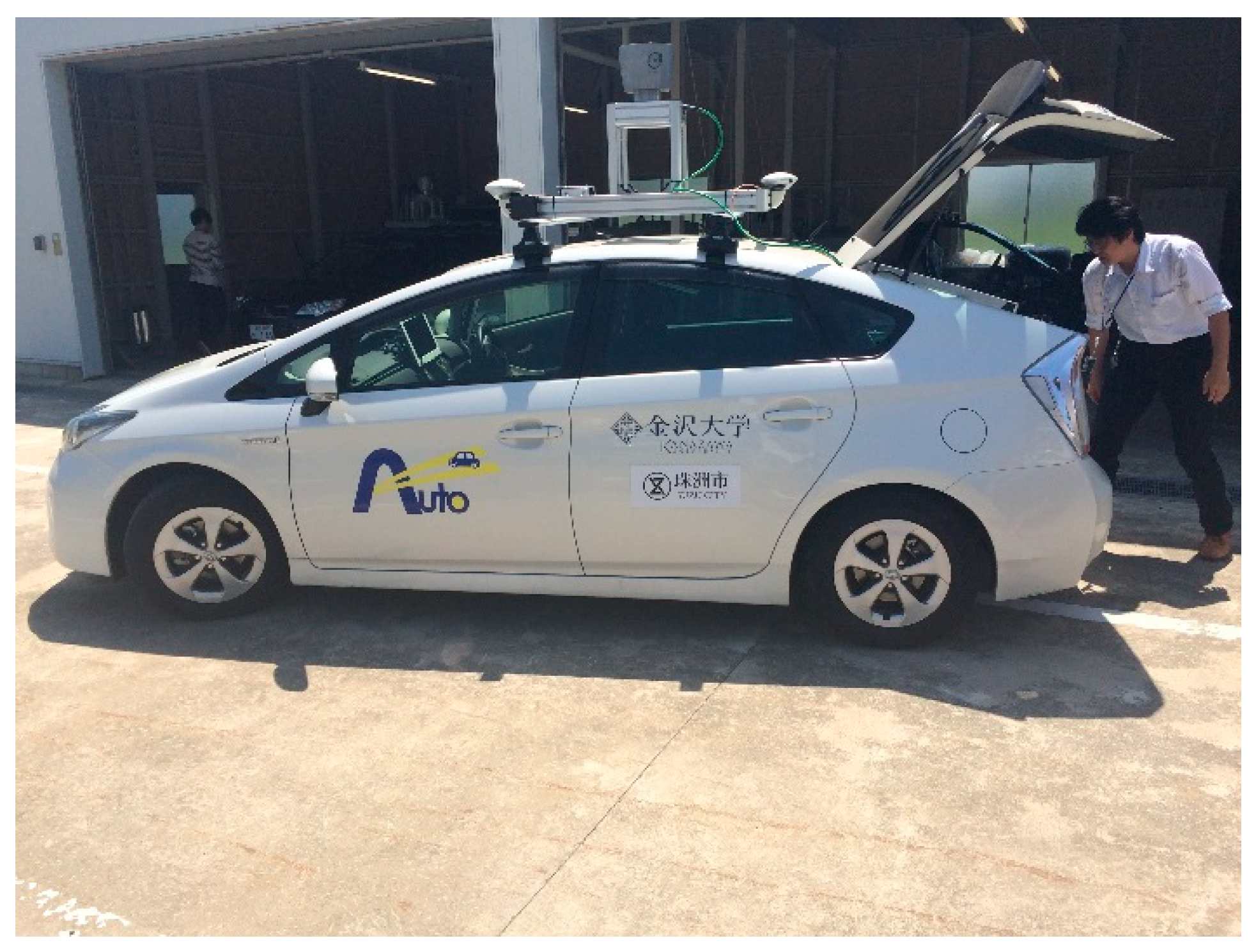
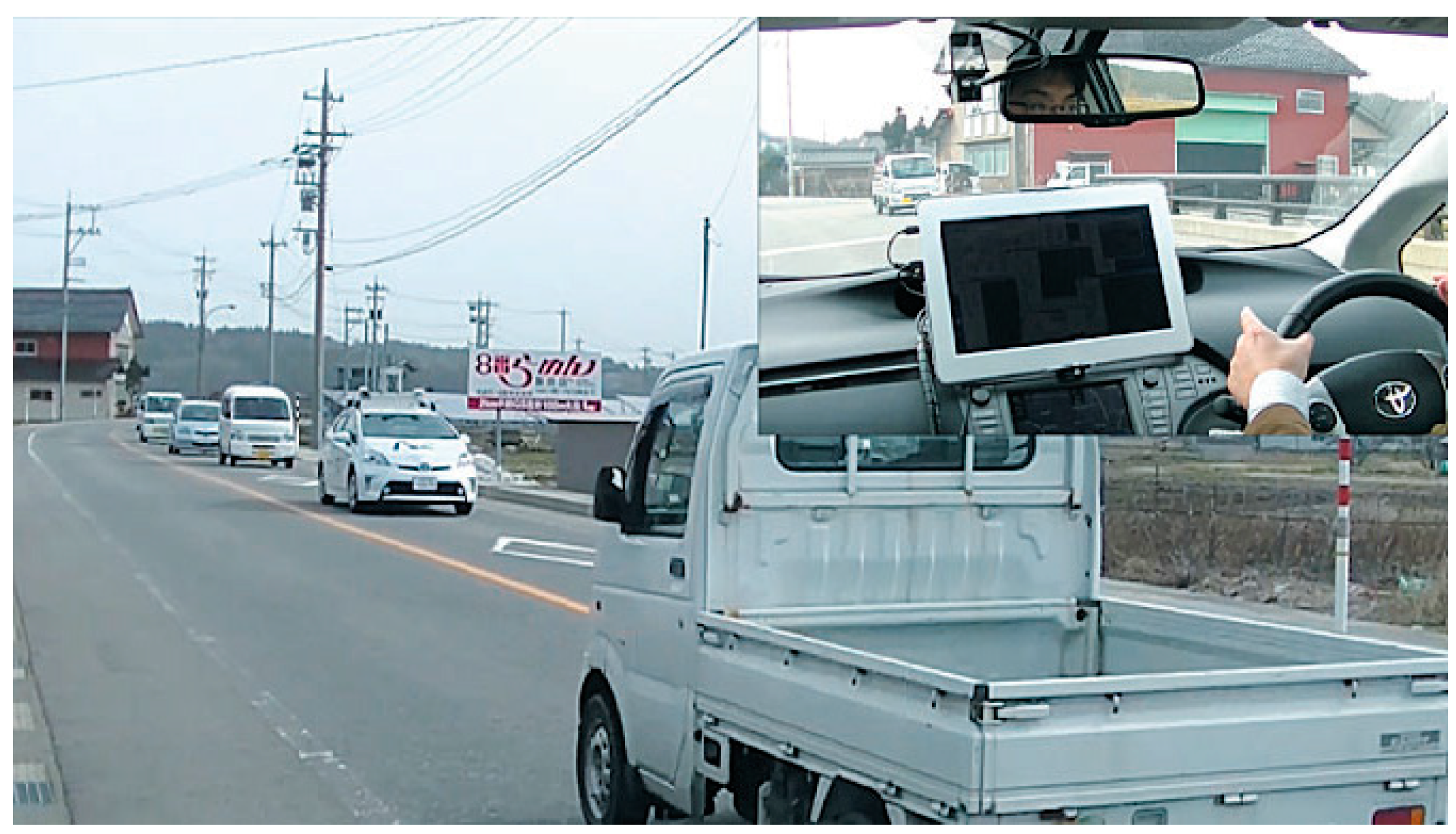
2.2. Demonstration Experiment in Suzu City, Japan

Here, we discuss a driving experiment involving an autonomous vehicle on public roads in Suzu City, Ishikawa Prefecture, which is the first reported attempt by any Japanese university (Figure 2). Suzu City is an aging municipality located at the tip of Noto Peninsula in Ishikawa Prefecture, with 45% of its population (15,000) being elderly. Presently, public transportation in Suzu City is limited to buses and taxis, and depending on the specific area, there may be only one bus service per day. Therefore, the use of autonomous vehicles to service areas without public transportation is urgently required. Driving tests in Suzu City began in February 2015, and it is currently in the initial stage of the experiment. The experiment aims to improve elemental technology of autonomous driving such as recognizing driving environments and pass planning, and this is being carried out primarily by accumulating driving data from urban areas. In the future, we plan to continue our tests towards the utilization of autonomous vehicles in Suzu City as part of its public transportation network. The vehicle used for the experiment is the Toyota Prius shown in Figure 1, and it has been remodeled so that the steering angle, braking, driving, and turning signals can be controlled using commands received from a computer. Upon installing various sensors, experiments were performed on public roads after confirming that no traffic regulations would be breached. At the present time, the section used for the driving experiment is about 6.6 km in various environments such as urban areas and mountainous areas. In April 2015, two months after the beginning of the experiment, a completely autonomous return journey was successfully achieved, with a total distance of 13.2 km. Figure 2 shows some pictures taken during the driving experiment. From the driving experiment, we also discovered various issues related to urban areas. For example, there is a problem with the sensor layout. In the test vehicle that we are currently using for the driving experiment, we installed a laser-range sensor that is able to sense all directions. However, since the sensor was installed in the center of the vehicle, in intersections with poor visibility, the condition of such an intersection cannot be safely assessed unless the vehicle has already entered the intersection. Normally, drivers can confirm the condition of an intersection with limited view by moving their heads; however, this is not possible with the sensor that was fixed to the vehicle. Therefore, an omnidirectional sensor is insufficient, and it is important to place the sensor in a position that allows for the appropriate monitoring of critical regions. By driving on public roads, other problems, both significant and minor, were highlighted. To fully understand these findings, a public road driving test is essential. As such, the autonomous vehicle that is presently being studied continues to go through driving experiments on public roads, while we continue to develop fundamental technologies.

3. Evaluation of Social Acceptability of Autonomous Vehicles

3.1. Execution Environment of the Simulation

In this study, we used Aimsun 8.0 to evaluate the impact of autonomous vehicles on traffic flow. To express the behavior of autonomous vehicles, we used C++ on the Aimsun SDK platform. Aimsun is a high-function traffic simulator that is considered one of the best worldwide, and it was developed by a Spanish company, TSS (Barcelona, Spain). It is a comprehensive traffic-simulation platform that is able to handle microsimulations, mesosimulations, hybrid simulations, and traffic-demand models together in one application. Aimsun allows for the selection of the origin–destination (OD) model or the branching rate model depending on the situation. With the OD model, without assumed conditions such as the branching rate, we can perform a simulation using path selection.

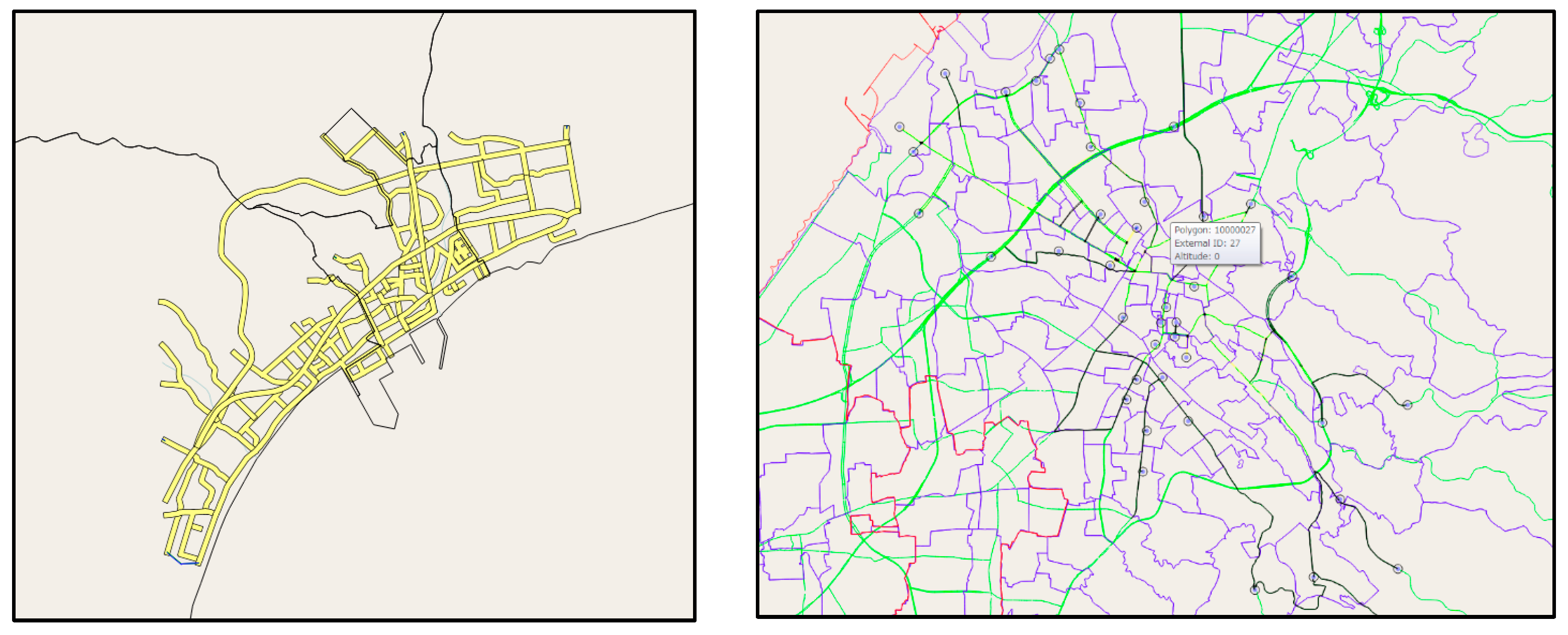
3.2. Simulation Area

Kanazawa City is a major city in Ishikawa Prefecture, with an area of 467.8 km2 and a population of 454,607. The use of cars accounts for 67.2% of the modes of transportation employed, and this is 22.5% higher than the national average of 44.7%. The main mode of public transportation is the bus (4.6%), with higher usage by the elderly in the center of the city. Based on these facts, it is a city with a relatively advanced degree of motorization of urban areas. With respect to aging, in 2013, 23.3% of the total population was at least 65 years of age, and this figure is expected to rise to 28.6% by 2025. On the other hand, Suzu City is a rural city in Ishikawa Prefecture with an area of 247.2 km2 and a population of 14,631. Within the city, there are no forms of public transportation, such as trains and buses, and residents mainly travel by car. In 2015, 46.6% of the total population was at least 65 years of age, and this figure is expected to rise to 51.7% in 2025 (Figure 3).

3.3. Simulation Data

In this section, we present various data used for the simulation. First, we assumed the traffic flow based on the 2005 person-trip (PT) survey. PT surveys examine “when”, “from where”, “to where”, “who”, “for what reason”, and “what transportation method”, and capture the movements of persons throughout a given day. The target city is divided into zones, and the OD traffic volumes in these zones are surveyed. In the present simulation, the authors superimposed zones used for the PT survey on the road data prepared using a digital road map (DRM) using GIS data. We placed a centroid (the point where vehicles gather and begin) and prepared the OD model for each zone. In this study, the current conditions were reproduced according to the traffic flow of the Parson trip survey conducted by the government. The centroid was set so that the centroid would have the highest result from the as-built simulation. The OD settings during the simulation were set using the Parson trip survey. The route selection model used was the model provided by the traffic flow simulation system (Aimsun). Using Aimsun, by preparing an OD table, the vehicle distribution on the OD base can be performed; therefore, we set each centroid to match the zone number of the PT survey and prepared the OD table. Next, we used the 2010 traffic census for Suzu City. A traffic census is a national statistical survey that is conducted to understand the roads and traffic in a region, and it aims to obtain basic information on road plans, construction, and management. The main data survey the cross-sectional traffic volume over a certain section of the road. Because the simulation area of Suzu City is relatively small, and the traffic volume distribution in the PT survey zone was complex, we used the traffic census in this study. For the transportation network, we prepared the roads at the prefectural level (highways and main thoroughfares that connect important areas within the prefecture). It is currently difficult to traverse narrow streets with the present autonomous vehicle technology, but because the simulation is in the OD base and the target vehicle may pass through narrow streets, we omitted such narrow streets for convenience. The simulation was performed for the one-hour period from 8 to 9 a.m., which is when congestion is likely to occur. The time of the simulations in this study was aligned with the time of the Parson trip survey. In this study, the results of the Parson trip survey were used to reproduce the current state of traffic volumes on the simulation and the survey results. As a result, the simulation results were 95% accurate in matching the current traffic volume with the simulated traffic volume. These conditions were evaluated by mixing autonomous vehicles. This is to minimize the impact of passing traffic that cannot be accommodated by the PT survey OD traffic volume, while observing the change in congestion. The number of vehicles was 10,274 in Kanazawa City and 1025 in Suzu City.

3.4. Driving Behavior Algorithm of Autonomous Vehicle

In Aimsun, we used the following Gipps formula for the vehicle behavioral algorithm, which is shown below [35,36,37,38,39,40,41,42]:

3.4.1. Car-Following Theory

V a ( n , t + T ) = V ( n , t ) + 2.5 a ( n ) T ( 1 V ( n , t ) V e ( n ) 0.025 + V ( n , t ) V e ( n ) )
Va: Speed of vehicle a;
V(n, t): Speed of vehicle n at time t;
Ve(n): Expected velocity of vehicle n;
a(n): Maximum acceleration of vehicle n;
T: Reaction speed of the driver.
V b ( n , t + T ) = d ( n ) + d ( n ) 2 T 2 d ( n ) 2 x ( n 1 , t ) s ( s 1 ) x ( n , t ) V ( n , t ) T V ( n , t ) 2 d ( n 1 )
Vb: Speed of vehicle b;
d(n): Maximum deceleration of vehicle n;
x(n, t): Position of vehicle n at time t;
s(n − 1): Length of vehicle n − 1;
d′(n − 1): Expected deceleration of vehicle n − 1.
We compared the values obtained using the above two equations, and we used the smaller one. The velocity of the autonomous vehicle depends on the distance to the vehicle driving in front.

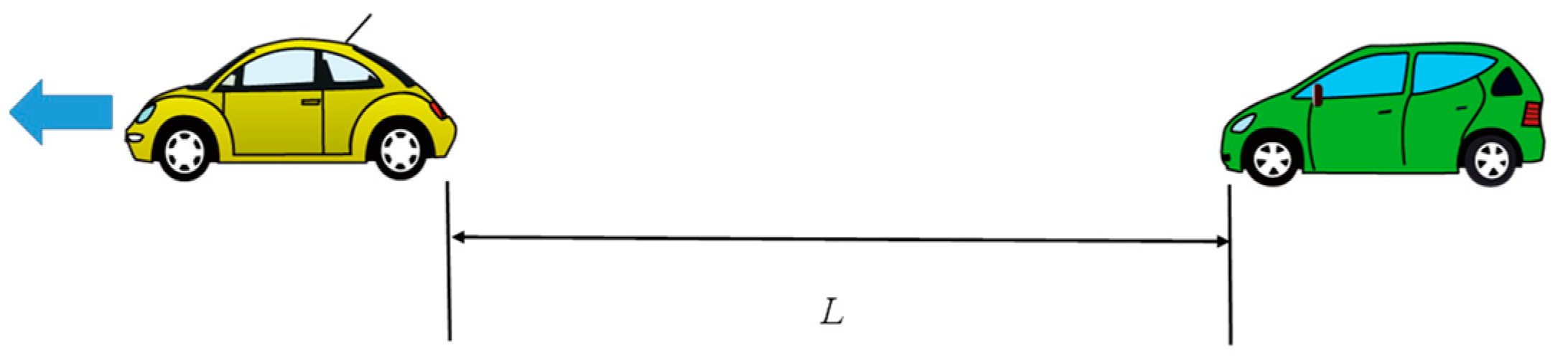
3.4.2. Vehicle Interval

The formula used to determine the vehicle spacing in Aimsun is shown below. Equation (3) shows the interval between vehicles. Thus, V1 represents the speed of the car in front; V2 represents the speed of the car behind.
V e h i c l e I n t e r v a l = V 2 2 2 b V 1 2 2 b + 1.5 V 2 R T L
b: deceleration;
RT: reaction speed;
L: vehicle length + minimum distance from vehicle in front when the car is at rest.
We determined the vehicle interval for autonomous vehicle (Figure 4) in this study is determined with the following equation:
V e h i c l e I n t e r v a l = 5 + V a × T T C
Va: velocity of vehicle driving in front;
TTC (time to collision): distance from the vehicle in front divided by the relative velocity.
For the autonomous vehicle in this study, TTC is assumed to be 2 s.

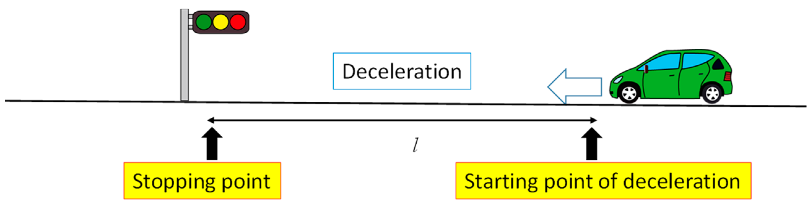
3.4.3. Deceleration Starting Distance

If the distance from the deceleration starting point to the stopping point is l (Figure 5), this is calculated using the following equation, and the vehicle will begin to decelerate so that it can come to a stop within the predetermined deceleration.
l = 1 2 a V 2

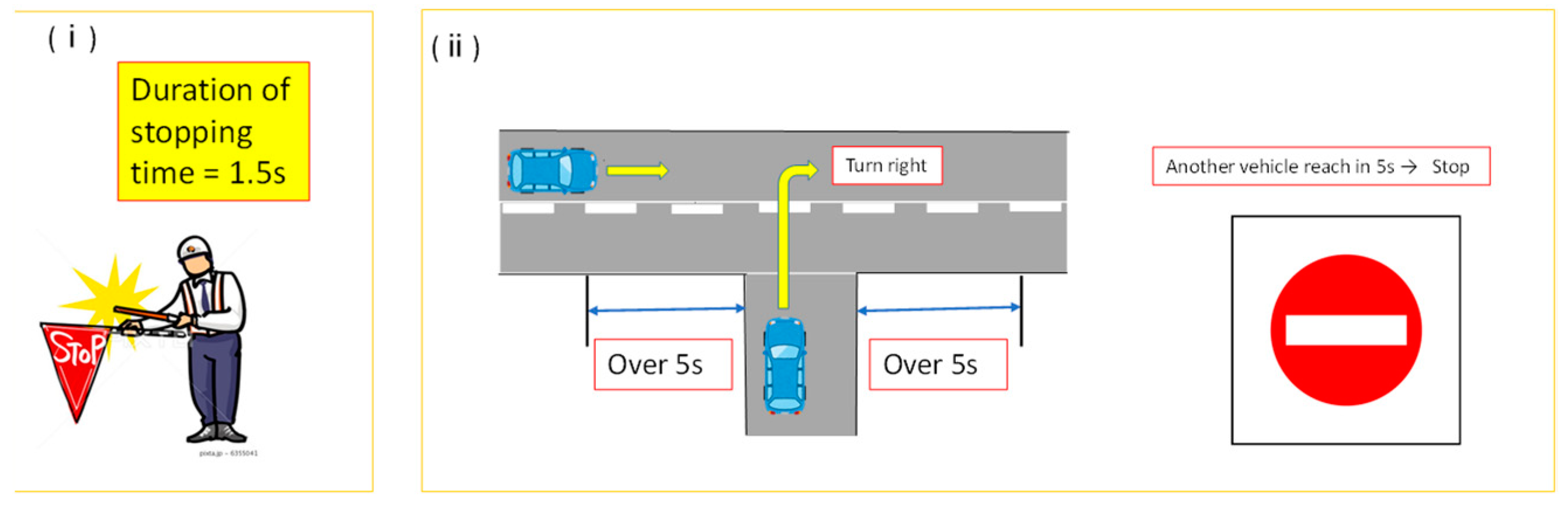
3.4.4. Determining When to Turn Right or Left

The vehicle begins to turn right or left when the following conditions are met. In this study, the setting for determination of left turns and right turns was based on observations of traffic flow (Figure 6).
At least 1.5 s has elapsed since coming to a stop as shown in Figure 6i.
If there is no oncoming vehicle on the driving route within 5 s, the vehicle will start as shown in Figure 6ii.

3.4.5. Reaction Time

In this study, we set the reaction time based on the environment surrounding the driver in the simulation system. General vehicles have a reaction time of 0.8 s during normal operation, 1.2 s when stopping, and 1.6 s to the vehicle in front. However, vehicles driven by the elderly have reaction times of 1.6 s during normal operation, 2.4 s when stopping, and 3.2 s to the vehicle in front (modeling reaction time within a traffic simulation model).

4. Results and Discussion

In this study, Suzu City and Kanazawa City were selected for the following reasons. Presently, the driving experiments of the autonomous vehicle owned by Kanazawa University are being conducted in Suzu City, and social implementation is therefore expected to be relatively fast. We aim to determine whether there is a difference in the impact on traffic flow between a rural area such as Suzu City and an urban area such as Kanazawa City. The present simulation gradually increases the mixing rate of autonomous vehicles. It is assumed that autonomous vehicles have become commercially available to the general public, and an increase in the number of such vehicles is captured over time. As it increases, the changes in the traffic congestion are observed, and we observe whether the impact of the autonomous vehicle is positive or negative, using the delay time as a parameter. This delay time is the difference between the expected time of arrival for the autonomous vehicle and the actual arrival time for each 1 km of roadway. By comparing these value, we determine the degree of congestion. On the graph, the vertical axis shows the delay time, while the horizontal axis shows the mixing rate. We also compared the delay time for the operations of general vehicles and autonomous vehicles to observe the potential trends in changes in delay time owing to vehicle characteristics.

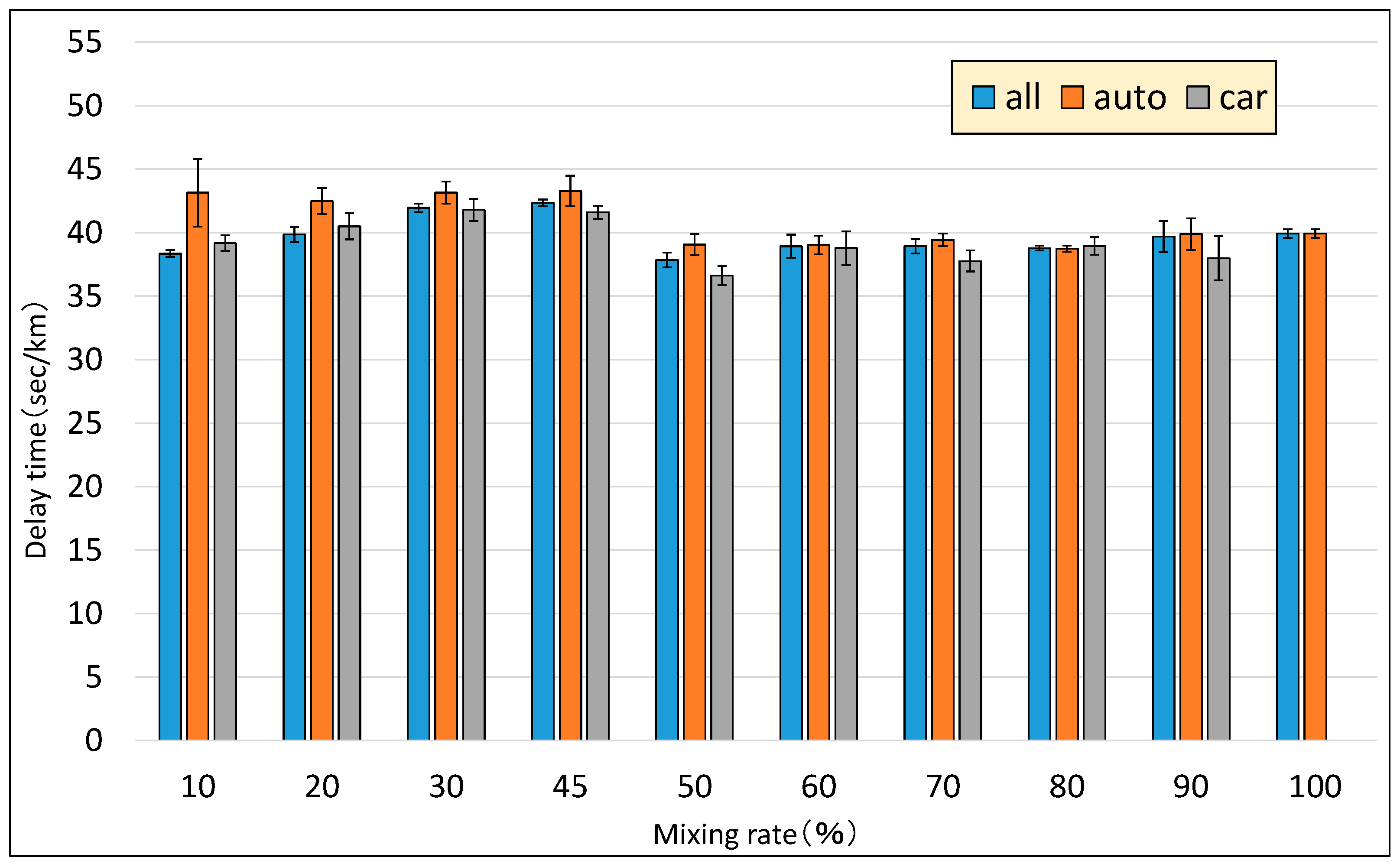
4.1. Simulation Results for Rural Areas

First, we considered the lack of public transportation and high ratio of the elderly population in Suzu City. We prepared a vehicle with a reaction time that is slower than that of a general vehicle and used a mixing rate of 45% based on the actual ratio of seniors in Suzu City. The mixing rates of the autonomous vehicle in the simulation were 10%, 20%, 30%, 45%, 50%, 60%, 70%, 80%, 90%, and 100%. Each mixing rate was verified three times. In this study, we used the mean delay time obtained from each of the three verifications (three patterns of delay for each mixing rate) as the delay time for each mixing rate. Figure 7 shows simulation results obtained for Suzu City. The blue bars in Figure 7 represent the delay time for all vehicles including both autonomous and general vehicles. Red bars represent the delay time for only autonomous vehicles for each mixing rate. Grey bars represent the delay time for only general vehicles for each mixing rate. The standard deviation for each delay time obtained from three delay patterns is also shown in Figure 7. The reason for which there is no 0% mixing rate is because the delay time is calculated with a standard value, and in the present study, the standard is when there are no autonomous vehicles, i.e., a 0% mixing rate. This study used representative values from a person-trip survey conducted by the local government, and although the results are of a general nature, they show the traffic situation in a rural area (Suzu City), especially in a situation where the traffic density is extremely low.
Furthermore, with a mixing rate of 100%, there is no delay time for general vehicles. This is because when the mixing rate of autonomous vehicles is 100%, there are no general vehicles, and thus there would be no delay.
Figure 7 shows that the delay time for all vehicles slightly increases as the mixing rate of autonomous vehicles increased from 10 to 45%. When the mixing rate increased from 45 to 50%, the delay time for all vehicles decreased notably, and when the mixing rate was 50 to 100%, it remained constant. Next, we compare the 10% and 45% mixing rates, between which the delay time increased. The delay time at the mixing rate of 45% was 1.10 times that at the mixing rate of 10%. The delay time dropped by 0.89 from the mixing rate of 45% to 50%. The delay time of the autonomous vehicle for each mixing rate was different from the delay time of all vehicles when the mixing rate increased from 10 to 45% and remained mostly the same. When the mixing rate increased from 45 to 50%, the delay time suddenly dropped and plateaued.
The delay time of general vehicles for each mixing rate increased at a mixing rate of 10 to 45% and then suddenly dropped at 45–50%, then remained constant, which was the same trend observed for the delay time of all vehicles.

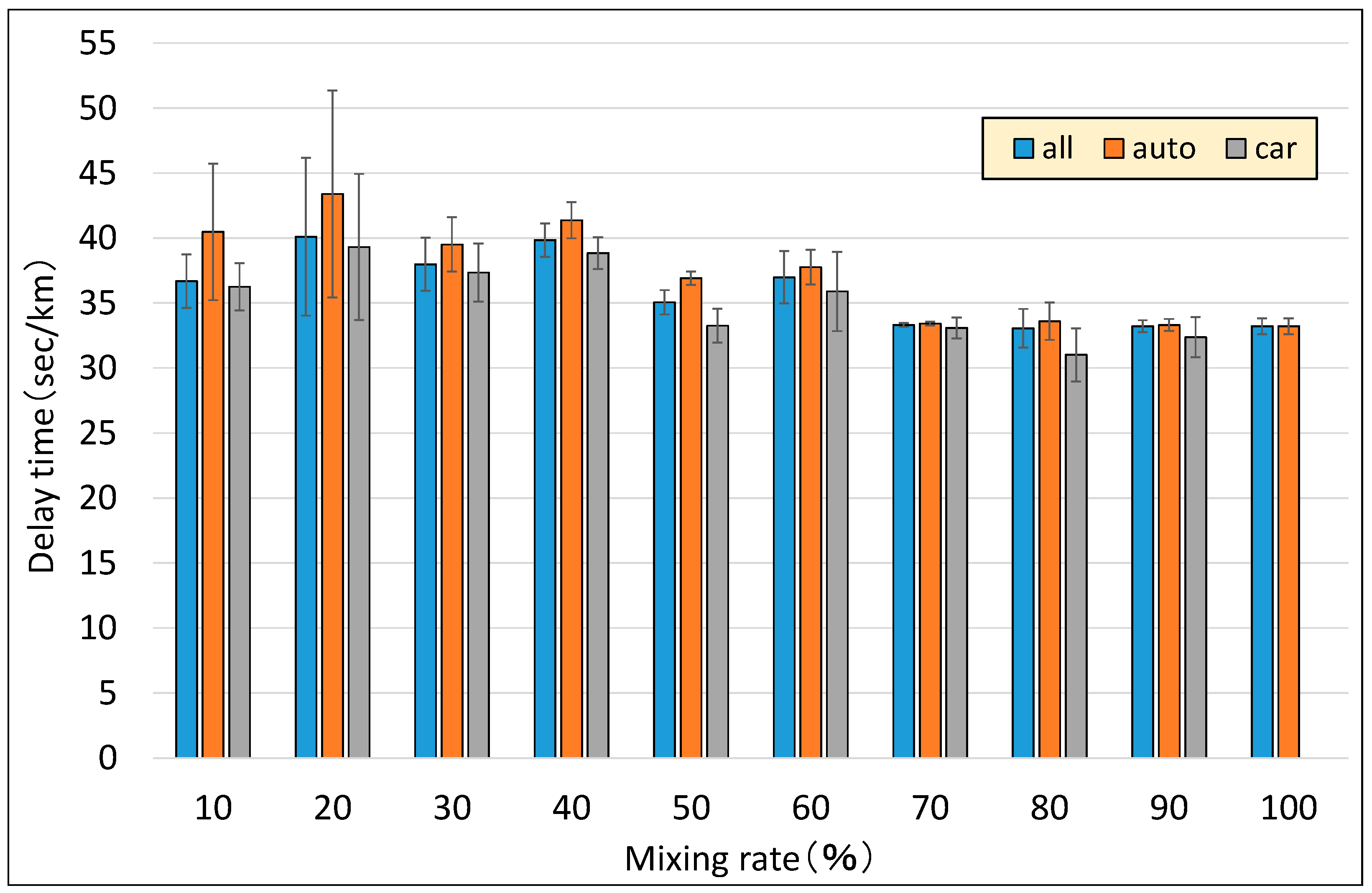
4.2. Simulation Results for Urban Areas

Next, we performed the simulation for Kanazawa City, and verifications were carried out in the same manner as in Suzu City. Figure 8 shows the simulation results for Kanazawa City. The trend details for Figure 8 are the same as those of Figure 7. Figure 8 shows that the delay time for all vehicles fluctuated between mixing rates of 10 to 60%. The standard deviation also showed variations. When the mixing rate increased from 60 to 70%, the delay time for all vehicles decreased, then remained constant without large variation. We focused on the mixing rate of 60 and 70% when the delay time decreased and stabilized and found that the delay time changed by a factor of 0.90 from the mixing rate of 60% to 70%. The delay time for the autonomous vehicle for each mixing rate had the same trend as that of all vehicles. Similar to the delay time for all vehicles, as the mixing rate increased from 60% to 70%, the delay time decreased, and then remained constant. By comparing the mixing rates of 60% and 70%, the delay time decreased by a factor of 0.89. The delay time for general vehicles also fluctuated between the mixing rates of 10% and 60%, and it showed a minor decrease from 60% to 70%, after which it stabilized. Between the mixing rates of 60% and 70% where the delay time decreased and stabilized, compared with the other two patterns, the delay time decreased the least by 0.92. When the mixing rate of automated vehicles is low, the delay time tends to be large because of the negative impact on traffic flow. On the other hand, when the mixing rate of automated vehicles is high, the delay time tends to be smaller than when the mixing rate is low. Based on these results, there is concern that the delay time will be significantly larger than the current situation unless the mixing rate is controlled to be 70% or higher when taking measures to introduce automated vehicles.

5. Conclusions

In this study, we used a traffic flow simulation system, and we evaluated the impact on the traffic flow using the delay time between the OD when an autonomous vehicle is socially implemented. We evaluated the effects on the traffic flow in an urban area that has been motorized and in an aging rural area. For both areas, with the implementation of the autonomous vehicle, decreased congestion, decreased traffic accidents, and the improved reliability of travel time are expected. However, as the population of rural areas is aging and these regions becoming more sparsely populated, its implementation may be able to solve many issues such as mobility for seniors.
We examined an autonomous vehicle that is being developed by our university. The autonomous vehicle that was employed is equipped with various sensors and is able to drive on public roads with complete autonomy. In order to evaluate the impact on the traffic flow, we developed an algorithm to incorporate its driving behavior into a traffic flow simulation system. This algorithm consists of car-following, vehicle intervals, principle start position, right/left turn decision, and reaction time to environmental changes.
We implemented into the traffic flow simulation system the autonomous vehicle algorithm that we developed in this study, and we modeled an environment that allows for simulations with autonomous vehicles. In a traffic flow simulation system, based on the results of PT surveys and transportation census, the OD traffic volume was determined, and a normal traffic environment was modeled. Next, the autonomous vehicle was driven and its impact on traffic flow was evaluated. In this study, to evaluate the impact of the autonomous vehicle on traffic flow, we used the delay time between OD as an indicator. We increased the mixing rate of autonomous vehicles in the traffic environment in increments of 10%, and we obtained the delay time between the OD.
When we compared the results for Kanazawa City and Suzu City, the delay time for all vehicles was found to be smaller in Kanazawa City. The variations in the delay time due to the increasing mixing rate were more notable in Kanazawa City, while it was more stable in Suzu City. This was likely because of differences in the road characteristics of both cities, such as the number of intersections and traffic volume. During the initial stages of the vehicles’ implementation in the society, traffic congestion may increase. However, when the ratio exceeds a certain value, congestion is expected to decrease and the traffic environment will improve.
As such, when autonomous vehicles are mixed with general vehicular traffic, there is some impact on traffic flow. It has been shown that the impact of autonomous vehicles on traffic flow depends greatly on the mixing rate and traffic environment, such as urban or rural areas. Because the mixing rate of autonomous vehicles impacts the traffic flow when socially implementing autonomous vehicles, appropriate distribution scenarios and distribution areas are necessary.
In this study, we recreated the implementation of a specific autonomous vehicle in a traffic flow simulation system, and we evaluated the impact on traffic flow using the delay time between OD, which is an evaluation indicator. To evaluate in more detail the impact of the social implementation of autonomous vehicles on traffic flow, the driving behaviors of all autonomous vehicles being developed worldwide need to be recreated in the traffic flow simulation system to consider the variety of autonomous vehicles. Furthermore, in this study, we recreated the traffic environments of an urban area and a rural area in the traffic flow simulation, but the system only considers vehicles. Therefore, the right- or left-turning behaviors of autonomous vehicles in the traffic flow simulation system were not complex. However, considering non-vehicular traffic, such as pedestrians and cyclists, the autonomous vehicle will need to make many decisions before turning right or left, making such decisions more complex. As a result, the delay time between the OD may increase. In this study, we evaluated the impact of the social implementation of autonomous vehicles on traffic flow using the delay time between OD. However, various other evaluation indicators need to be applied to evaluate the impact of social implementation of autonomous vehicles on traffic flow. Therefore, we have added a note in the future issues section of the manuscript that although this study uses only delay time as an evaluation index, it is necessary to evaluate the impact on traffic flow using evaluation indexes other than delay time in the future. In this study, the analysis was conducted during weekday morning hours. However, it is necessary to target the traffic environment on weekends and holidays, as well as the evening peak hours. In this study, based on the results of a person-trip study conducted by the government, we evaluated the basic impact of the mixing of automated vehicles into the normal traffic flow by using the mixing rate and the delay time of automated vehicles. However, the results of this study were based on limited parameter settings, so future sensitivity analyses should be conducted by varying the various parameters used in this study to evaluate the impact of automated vehicles when they are mixed into various traffic environments from a multifaceted perspective. In the future, it will be necessary to study the method of dispatching automated vehicles, the areas where they will be used, traffic flow management and planning, etc., in order to make them practical. Due to the limitation of the simulation system, the evaluation in this study was based on the delay time. Simulation experiments under various conditions are necessary to generalize the results of this study.

Author Contributions

Conceptualization, M.F. and J.T.; methodology, M.F.; software, M.F. and Y.M.; validation, M.F., Y.M. and J.T.; formal analysis, M.F. and Y.M.; investigation, Y.M.; resources, M.F., Y.M. and J.T.; data curation, M.F., Y.M. and J.T.; writing—original draft preparation, M.F.; writing—review and editing, M.F.; visualization, M.F. and Y.M.; supervision, J.T.; project administration, J.T.; funding acquisition, M.F. All authors have read and agreed to the published version of the manuscript.

Funding

This research received no external funding.

Institutional Review Board Statement

Not applicable.

Informed Consent Statement

Not applicable.

Data Availability Statement

Data are contained within the article.

Conflicts of Interest

The authors declare no conflict of interest.

References

  1. Khodayari, A.; Ghaffari, A.; Ameli, S.; Flahatgar, J. A Historical Review on Lateral and Longitudinal Control of Autonomous Vehicle Motions. In Proceedings of the 2010 2nd International Conference on Mechanical and Electrical Technology (ICMET), Singapore, 10–12 September 2010. [Google Scholar] [CrossRef]
  2. Fagnant, D.J.; Kockelman, K. Forecasting Americans’ Long-term Adoption of Connected and Autonomous Vehicle Technologies. Transp. Res. Part A Policy Pract. 2015, 77, 164–181. [Google Scholar]
  3. Bansal, P.; Kockelman, K.M. Preparing a Nation for Autonomous Vehicles: Opportunities, Barriers and Policy Recommendations. Transp. Res. Part A Policy Pract. 2017, 95, 49–63. [Google Scholar] [CrossRef]
  4. Levin, M.W.; Boyles, S.D. A Multiclass Cell Transmission Model for Shared Human and Autonomous Vehicle Roads. Transp. Res. Part C Emerg. Technol. 2016, 62, 103–116. [Google Scholar] [CrossRef]
  5. Beiker, S.A. Legal Aspects of Autonomous Driving. Santa Clara Law Rev. 2016, 52, 1145. [Google Scholar] [CrossRef]
  6. Levin, M.W.; Boyles, S.D. A Cell Transmission Model for Dynamic Lane Reversal with Autonomous Vehicles. Transp. Res. Part C Emerg. Technol. 2016, 68, 126–143. [Google Scholar] [CrossRef]
  7. Chen, T.D.; Kockelman, K.M. Management of a Shared Autonomous ElectricVehicle Fleet Implications of Pricing Schemes. Transp. Res. Rec. J. Transp. Res. Board 2016, 2572, 37–46. [Google Scholar] [CrossRef]
  8. Bimbraw, K. Autonomous Cars: Past, Present and Future a Review of the Developments in the Last Century, the Present Scenario and the Expected Future of Autonomous Vehicle Technology. In Proceedings of the 12th International Conference on Informatics in Control, Automation and Robotics (ICINCO), Colmar, France, 21–23 July 2015. [Google Scholar]
  9. Bonnefon, J.-F.; Shariff, A.; Rahwan, I. The Social Dilemma of Autonomous Vehicles. Science 2016, 352, 1573–1576. [Google Scholar] [CrossRef] [PubMed]
  10. Kalra, N.; Paddock, S.M. Driving to Safety: How Many Miles of Driving Would it Take to Demonstrate Autonomous Vehicle Reliability? Transp. Res. Part A Policy Pract. 2016, 94, 182–193. [Google Scholar] [CrossRef]
  11. Chen, T.D.; Kockelman, K.M.; Hanna, J.P. Operations of a Shared, Autonomous, Electric Vehicle fleet: Implications of Vehicle and Charging Infrastructure Decisions. Transp. Res. Part A Policy Pract. 2016, 94, 243–254. [Google Scholar] [CrossRef]
  12. Fagnant, D.J.; Kockelman, K.M. The Travel and Environmental Implications of Shared Autonomous Vehicles, Using Agent-based Model Scenarios. Transp. Res. Part C Emerg. Technol. 2014, 40, 1–13. [Google Scholar] [CrossRef]
  13. Gucwa, M. Mobility and Energy Impacts of Automated Cars. In Proceedings of the Automated Vehicles Symposium, Burlingame, CA, USA, 15–17 July 2014. [Google Scholar]
  14. Hoogendoorn, R.; van Arerm, B.; Hoogendoom, S. Automated Driving, Traffic Flow Efficiency, and Human Factors Literature Review. Transp. Res. Rec. J. Transp. Res. Board 2014, 2422, 113–120. [Google Scholar] [CrossRef]
  15. Campbell, M.; Egerstedt, M.; How, J.P.; Murray, R.M. Autonomous Driving in Urban Environments: Approaches, Lessons, and Challenges. Philos. Trans. R. Soc. A Math. Phys. Eng. Sci. 2010, 368, 4649–4672. [Google Scholar] [CrossRef]
  16. How, J.P.; Behihke, B.; Frank, A.; Dale, D.; Vian, J. Real-time Indoor Autonomous Vehicle Test Environment. IEEE Control Syst. 2008, 28, 51–64. [Google Scholar] [CrossRef]
  17. Howard, A. Real-time Stereo Visual Odometry for Autonomous Ground Vehicles. In Proceedings of the IEEE/RSJ International Conference on Intelligent Robots and Systems, IROS 2008, Nice, France, 22–26 September 2008; pp. 3946–3952. [Google Scholar]
  18. Kuwata, Y.; Teo, J.; Fiore, G.; Karaman, S.; Frazzoli, E.; How, J.P. Real-Time Motion Planning with Applications to Autonomous Urban Driving. EEE Trans. Control Syst. Technol. 2009, 17, 1105–1118. [Google Scholar] [CrossRef]
  19. Fernandes, P.; Nunes, U. Platooning of Autonomous Vehicles with Intervehicle Communications in SUMO Traffic Simulator. In Proceedings of the 13th International IEEE Conference on Intelligent Transportation Systems (ITSC), Funchal, Portugal, 19–22 September 2010. [Google Scholar] [CrossRef]
  20. Douglas, A.R.; Shafer, S.A. Computational Model of Driving for Autonomous Vehicles. Transp. Res. Part A Policy Pract. 1993, 27, 23–50. [Google Scholar]
  21. Vine, S.L.; Zolfaghari, A.; Polak, J. Autonomous Cars: The Tension between Occupant Experience and Intersection Capacity. Transp. Res. Part C Emerg. Technol. 2015, 52, 1–14. [Google Scholar] [CrossRef]
  22. Khalaji, A.K.; Moosavian, S.A.A. Dynamic Modeling and Tracking Control of a Car with n trailers. Multibody Syst. Dyn. 2016, 37, 211–225. [Google Scholar] [CrossRef]
  23. Bose, A.; Ioannou, P. Analysis of Traffic Flow with Mixed Manual and Semiautomated Vehicles. IEEE Trans. Intell. Transp. Syst. 2003, 4, 173–188. [Google Scholar] [CrossRef]
  24. Michael, J.B.; Godbole, D.N.; Lygeros, J.; Sengupta, R. Capacity Analysis of Traffic Flow Over a Single-Lane Automated Highway System. ITS J. Intell. Transp. Syst. 1998, 4, 49–80. [Google Scholar] [CrossRef]
  25. Basak, K.; Hetu, S.N.; Li, Z.; Azevedo, C.L.; Loganathan, H.; Toledo, T.; Xu, R.; Xu, Y.; Peh, L.S.; Ben-Akiva, M. Modeling Reaction Time within a Traffic Simulation Model. In Proceedings of the 2013 16th International IEEE Conference on Intelligent Transportation Systems (ITSC), The Hague, The Netherlands, 6–9 October 2013. [Google Scholar]
  26. Sun, L.; Cheng, Z.; Kong, D.; Xu, Y.; Wen, S.; Zhang, K. Modeling and analysis of human-machine mixed traffic flow considering the influence of the trust level toward autonomous vehicles. Simul. Model. Pract. Theory 2023, 125, 102741. [Google Scholar] [CrossRef]
  27. Gallo, M. Models, algorithms, and equilibrium conditions for the simulation of autonomous vehicles in exclusive and mixed traffic. Simul. Model. Pract. Theory 2023, 129, 102838. [Google Scholar] [CrossRef]
  28. Szarata, A.; Ostaszewski, P.; Mirzahossein, H. Simulating the impact of autonomous vehicles (AVs) on intersections traffic conditions using TRANSYT and PTV Vissim. Innov. Infrastruct. Solut. 2023, 8, 164. [Google Scholar] [CrossRef]
  29. Körtgen, C.; Abel, J.; Menzel, P. Simulation of Dense Traffic Situations to Validate Autonomous Driving Functions. ATZelectron. Worldw. 2022, 17, 48–52. [Google Scholar] [CrossRef]
  30. Tientrakool, P.; Ho, Y.-C.; Maxemchuk, N.F. Highway Capacity Benefits from Using Vehicle-to-Vehicle Communication and Sensors for Collision Avoidance. In Proceedings of the 2011 IEEE Vehicular Technology Conference (VTC Fall), San Francisco, CA, USA, 5–8 September 2011; pp. 1–5. [Google Scholar] [CrossRef]
  31. Chen, M.; Yi, M.; Huang, M.; Huang, G.; Ren, Y.; Liu, A. A novel deep policy gradient action quantization for trusted collaborative computation in intelligent vehicle networks. Expert Syst. Appl. Int. J. 2023, 221, 119743. [Google Scholar] [CrossRef]
  32. Liu, R.; Liu, A.; Qu, Z.; Xiong, N.N. An UAV-enabled intelligent connected transportation system with 6G communications for internet of vehicles. IEEE Trans. Intell. Transp. Syst. 2023, 24, 2045–2059. [Google Scholar] [CrossRef]
  33. Teng, H.; Dong, M.; Liu, Y.; Tian, W.; Liu, X. A low-cost physical location discovery scheme for large-scale Internet of Things in smart city through joint use of vehicles and UAVs. Futur. Gener. Comput. Syst. 2021, 118, 310–326. [Google Scholar] [CrossRef]
  34. Suganuma, N.; Yamamoto, D.; Yoneda, K. Localization for Autonomous Vehicle on Urban Roads. J. Adv. Control Autom. Robot. 2015, 1, 47–53. [Google Scholar]
  35. Ye, L.; Yamamoto, T. Evaluating the impact of connected and autonomous vehicles on traffic safety. Phys. A Stat. Mech. Its Appl. 2019, 526, 121009. [Google Scholar] [CrossRef]
  36. Yoneda, K.; Kuramoto, A.; Suganuma, N.; Asaka, T.; Aldibaja, M.; Yanase, R. Robust Traffic Light and Arrow Detection Using Digital Map with Spatial Prior Information for Automated Driving. Sensors 2020, 20, 1181. [Google Scholar] [CrossRef]
  37. Yoneda, K.; Hashimoto, N.; Yanase, R.; Aldibaja, M.; Suganuma, N. Vehicle Localization using 76 GHz Omnidirectional Millimeter-Wave Radar for Winter Automated Driving. In Proceedings of the 2018 IEEE Intelligent Vehicles Symposium, Changshu, China, 26–30 June 2018; pp. 971–977. [Google Scholar]
  38. Yoneda, K.; Suganuma, N.; Aldibaja, M. Simultaneous Sate Recognition for Multiple Traffic Signals on Urban Road. In Proceedings of the MECATRONICS-REM, Compiegne, France, 15–17 June 2016; pp. 135–140. [Google Scholar]
  39. Kuramoto, A.; Kameyama, J.; Yanase, R.; Aldibaja, M.; Kim, T.H.; Yoneda, K.; Suganuma, N. Digital Map Based Signal State Recognition of Far Traffic Lights with Low Brightness. In Proceedings of the 44th Annual Conference of the IEEE Industrial Electronics Society, Washington, DC, USA, 21–23 October 2018; pp. 5445–5450. [Google Scholar]
  40. Yamamoto, D.; Suganuma, N. Localization for Autonomous Driving on Urban Road. In Proceedings of the International Conference on Intelligent Informatics and BioMedical Sciences, Okinawa, Japan, 28–30 November 2015. [Google Scholar]
  41. Yoneda, K.; Yanase, R.; Aldibaja, M.; Suganuma, N.; Sato, K. Mono-Camera based vehicle localization using Lidar Intensity Map for automated driving. Artif. Life Robot. 2018, 24, 147–154. [Google Scholar] [CrossRef]
  42. Yoneda, K.; Suganuma, N.; Yanase, R.; Aldibaja, M. Automated driving recognition technologies for adverse weather conditions. IATSS Res. 2019, 43, 253–262. [Google Scholar] [CrossRef]
Figure 1. Autonomous vehicle owned by Kanazawa University.
Sustainability 16 00658 g001
Figure 2. Driving experiment on a public road.
Sustainability 16 00658 g002
Figure 3. Simulation network ((left): Suzu City; (right): Kanazawa City).
Sustainability 16 00658 g003
Figure 4. Vehicle spacing when going straight.
Sustainability 16 00658 g004
Figure 5. Stop condition when going straight.
Sustainability 16 00658 g005
Figure 6. Condition for turning right/left.
Sustainability 16 00658 g006
Figure 7. Simulation results for Suzu City (rural area in Ishikawa prefecture).
Sustainability 16 00658 g007
Figure 8. Simulation results for Kanazawa City.
Sustainability 16 00658 g008
Disclaimer/Publisher’s Note: The statements, opinions and data contained in all publications are solely those of the individual author(s) and contributor(s) and not of MDPI and/or the editor(s). MDPI and/or the editor(s) disclaim responsibility for any injury to people or property resulting from any ideas, methods, instructions or products referred to in the content.

