Article

Route Planning under Mobility Restrictions in the Palestinian Territories

1
Civil and Geo-Environmental Engineering Laboratory (LGCgE), Lille University, Rue Paul Duez, 59000 Lille, France
2
Department of Mechanical, Energy and Management Engineering, University of Calabria, Via Pietro Bucci, 46/C, 87036 Rende, Italy
3
University of Science and Technology of China, No.96, JinZhai Road Baohe District, Hefei 230026, China
4
Faculdade de Economia, Administração, Contabilidade e Atuária, University of São Paulo, Avenida Professor Luciano Gualberto, 908, Butantã 05508-010, SP, Brazil
*
Author to whom correspondence should be addressed.
Sustainability 2024, 16(2), 660; https://doi.org/10.3390/su16020660
Submission received: 1 December 2023 / Revised: 4 January 2024 / Accepted: 9 January 2024 / Published: 11 January 2024

Abstract

:
This study aims to enhance people’s mobility in the context of mobility restrictions in the Palestinian territories, West Bank. It aims to develop a comprehensive route planning model that prioritises safety and optimises travel time while also considering sustainability issues. Unlike previous research, which has often focused solely on traffic crashes and physical road considerations in safety route planning, this study addresses the gap by developing a comprehensive model that integrates new risk criteria including mobility restrictions and violent events. The methodology involves historical and real-time data collection and processing, machine learning-based travel time prediction, and route optimisation using Dijkstra’s algorithm. The results highlight the significant impact of violent incidents on comprehensive risk scores, offering insights for proactive, sustainable measures. The waiting time prediction model performs strongly, with (R-squared) R2 values ranging from 80% to 92%. The developed route planning model provides three categorised routes under mobility restrictions—safest, fastest, and shortest—offering travellers sustainable and tailored options.

1. Introduction

This paper presents a route planning model that considers, in a sustainable fashion, the mobility restrictions related to the occupation of the Palestinian territories in the West Bank (WB). Such constraints began about 30 years ago with the creation of permanent and temporary checkpoints [1,2], which have generated severe disturbances in the ordinary life of the population, with negative effects such as anxiety, physical risk, time losses, and unemployment [3]. These controls have also led to significant delays and non-sustainable issues due to transport route distance and time, generating high energy consumption and greenhouse gas emissions [4].
The West Bank population also faces mobility restrictions related to the settlers’ violence, ranging from road blockages to physical attacks. The United Nations Office for the Coordination of Humanitarian Affairs’ (OCHA) report indicated an unusual increase in settler violence for the year 2022, with an average of 6.6 injuries occurring daily [5]. Approximately 21% of settler-related incidents were linked to violence against vehicles, drivers, passengers, and road blockages [6]. This settler violence represents a severe risk that jeopardises mobility in Palestine and has the potential to cause physical harm and loss of life [7]. Consequently, safety became a major concern regarding social sustainability in the WB.
Recent studies have introduced safety as a pivotal parameter in route planning. For example, Sarraf and McGuire [8] developed a navigation system that considers the road segment’s safety level based on historical traffic crash data and a real-time monitoring system including the severity of crashes in terms of fatalities, injuries, and property damage. Similarly, Liao et al. [9] extended this approach to encompass driver, vehicle, road, and sustainability/environmental parameters. In contrast, Domínguez and Sanguino [10] developed a mobile app for pedestrian safety, factoring in elements like zebra crossings, pedestrian streets, and walkways.
A study by Noureddine and Ristic [11] in Serbia aimed to optimise routes for hazardous material transportation, taking into account traffic crashes, rail crossings, traffic congestion, and travel distance, as well as a risk profile of each individual involved in the transportation through a multi-criteria decision-making approach with scenario and sensitivity analysis. Likewise, Zandieh and Ghannadpour [12] expanded the scope of risk factors for efficiently managing hazardous material transportation to a more general context, implicitly including sustainability issues. The authors considered population density, vehicle load, link length, and time of the day using a type-2 fuzzy multi-objective evolutionary algorithm based on decomposition. Subotić et al. [13], in Serbia, focused on risks related to speed limit deviations that could be avoided by adopting a vehicle-differentiated speed limit framework—i.e., a more realistic and acceptable framework for road users. In Japan, specifically in the disaster-prone context of Kyoto, Wachtel et al. [14] proposed a framework for planning evacuation routes for tourists by gathering information about the transportation infrastructure and people’s behaviour. This study was based on a set of evacuation scenarios based on their predictability and the categories of information and data needed, the complexity of tourist flow monitoring and forecasting, and the actual data sources available. Additionally, Ikeda and Inoue [15] developed a general evacuation route planning model for post-natural disaster recovery, utilising a safety evaluation method that accounted for average walking speed, pedestrian traffic per hour, and distance between nodes. In detail, it helps with route planning by exploiting participatory sensing to estimate safe routes and to produce evacuation maps through GPS and accelerometer data from pedestrians’ smartphones and by implementing the Multi-Objective Genetic Algorithm (Moga).
Previous research [8,9,10,11,12,13] has focused on route planning safety related to traffic crashes and physical road networks. While violent incidents in the transportation system have attracted scholars’ attention since 2010 [16], existing research has highlighted the lack of studies on violence incidents in road-based route planning models.
Developed countries have reported high rates of violence against taxi drivers, ranging from 19% to 70%. For example, Turkey has a 35.2% rate of physical violence against taxi drivers [17]. Taxi driving in Australia is considered one of the riskiest professions, with at least one taxi driver being killed annually [18]. In 2019, the US reported over 1500 crime events in the transportation sector [19]. Alpkoçak and Cetin [20] addressed this violence by proposing a safe routing system based on historical crime data. However, this system is not well adapted to safety related to mobility restrictions.
Moreover, using the conventional risk indicators for safe route planning under mobility restrictions is inadequate. To cover this gap, this paper presents a comprehensive route planning model under mobility restrictions, including sustainability issues. This model is based on the following: (i) determining the risk score of a road section incorporating mobility restrictions, life-threatening violent events, built environment and sustainability at large, and road physical characteristics; (ii) the use of machine learning for the determination of the travel time under real-time restriction events.
The main contribution of this paper is to propose a solution for route planning that highlights safety issues while optimising travel times in areas suffering from mobility restrictions, violent incidents, bad road physical/lighting conditions, and proximity to built-up areas. It identifies multiple route categories: safest, fastest, and shortest route.
Additionally, the route planning model proposed in this study stands out from other models by offering users multiple route options such as safety, time, and emergency. This will cover the observed gap in the route planning solution that proposed a single optimal route, which may lead to congestion drift from the original route to the newly planned route, thus also impacting sustainability [21].
This paper uses the following definitions for route alternatives. The safest route designates the route that is not subjected to mobility restrictions and violence. The fastest route minimises travel time (and environmental sustainability impacts) while still ensuring users’ safety; thus, the fastest route is intended to be less time-consuming and also a safe route. The emergency route is the shortest route without considering the risk related to the mobility restrictions; thus, it offers the shortest path to reach a specific destination when the traveller is in an emergency situation (not considering other emergencies from authorities like evacuation orders or restriction/safety issues).
The remainder of this paper is structured as follows: Section 2 outlines of the materials and methods used for the route planning model. Section 3 describes the application of the methodology to the territorial context and the primary outcomes, and the limitations of this study and the conclusions that can be draw from it are provided in Section 4.

2. Materials and Methods

The methodology used to develop the route planning model consisted of two main stages. Firstly, it involved identifying the required data and the sources of these data. Secondly, it encompassed processing and analysing the data. This latter phase incorporates several components, including the following: (i) determining the risk score for the road sections, (ii) calculating the travel time (and implicitly sustainability) considering the predicted weighting time at the mobility restrictions, and (iii) creating a graph model that uses Dijkstra’s algorithm to find the safest, shortest, and fastest route. Figure 1 illustrates the research methodology phases.

2.1. Data Sources and Collection

The route planning model relies on the acquisition of both real-time and historical data concerning the road network and mobility restrictions. Real-time data were sourced from the SRMS platform, a web mobile application designed to share and map real-time location-based information about mobility restrictions such as checkpoints, road closures, traffic congestion, and incidents of violence, leveraging the concept of spatial crowdsourcing [22]. The spatial data generated by this platform are stored as a Web Feature Service (WFS), allowing for real-time access and geospatial data analysis via the Internet [23].
Historical data include information obtained from government transportation authorities, encompassing physical environmental data like road network geometry, road conditions, lighting, built-up areas, permanent mobility restrictions, and speed limits. Additionally, this includes open-source data derived from NGO reports documenting incidents of violence and historical waiting times at mobility restrictions. These historical data come in various spatial formats, including the shapefile format, which is a vector data storage format for GIS. Shapefiles store location, shape, and associated attributes [24]. They are also available in tabular and text formats. Table 1 provides a comprehensive overview of the data and sources needed for creating a route planning model.

2.2. Data Processing and Analysis

This phase consists of three steps to process and analyse the collected data to construct the route planning model. It includes (i) creating the risk score, (ii) calculating the travel time, and (iii) creating the route planning model to find multi-categorised routes.

2.2.1. Identifying the Risk Score

The risk score (Ri), in the realm of route planning problems, has been widely used in different studies. It assesses the overall level of risk associated with a particular route (Equation (1)). This score takes into account various factors related to safety, security, and the potential hazards that travellers may encounter along their route. One can determine the risk score by carrying out the following: (i) creating risk indicators and (ii) calculating the weight of each index.
R i = j = 1 m d i j w j
where Ri is the risk score of the ith road section (i = 1, 2, 3, ….n); dij is the actual data of the jth index corresponding to the ith road section; and wj is the weight of the jth index.
  • Creating risk indicators
The risk indicators incorporated in this study include the following: (i) the severity of violent incidents, (ii) mobility restrictions, and (iii) the physical road conditions and the built environment. The literature shows that the causes of violent actions can pertain to different aspects, include the following: a gender perspective, such as abusive practices against women [25]; the perspective of violence in the workplace, which is related to socioeconomic factors [26]; and the geopolitical perspective, which is represented by violent practices against civilians, especially in armed conflict areas [27].
In this study, violence refers to physical threats involving actual physical violence, such as using an object (stones, bottles, sticks, etc.) or a weapon against travellers [28]. This type of violence is prevalent in unstable geopolitical environments where there is a constant threat to people’s lives [27]. For example, Essenberg [29] showed that most road passenger transport sector workers in several conflict-prone countries have reported experiencing violence from armed forces, police officials, and customs agents at roadblocks or border posts.
The severity index was selected based on a literature review and reports discussing the severity of the violent actions directed towards travellers on the road. The index used to evaluate the severity of violent action against travellers on the route includes the number of previous violent acts [28] and the time the violence occurred [18]. The indices used to evaluate the physical road characteristics are the physical road condition and the road segment’s lighting condition [9], as well as the built environment (presented in the category of the adjacent built-up area to the road section) [30]. The number of mobility restrictions on the road section was used as an index for the mobility restriction criteria. Table 2 shows the evaluation criteria and the derived index for the risk on the road section. Notably, positive indexes—such as No_RIST, No_VIO, TOD, DOW, ROAD_CON, and ADJ_BUILTUP—reflect heightened risk levels with higher values. Conversely, LGT_CON assumes the negative, since a lack of adequate lighting might contribute to higher risks on the road due to reduced visibility.
  • Index weight calculation
The pre-identified indices’ contribution determines the comprehensive cost on the road section, based on their related weights. There are various weighting methods for the multi-criteria decision-making (MCDM) model, including subjective, objective, and combined methods [31,32]. Subjective methods like the Step-wise Weight Assessment Ratio Analysis (SWARA) method involve assigning weights based on expert or stakeholder opinions. In SWARA, decision makers compare criteria pairwise to determine their relative importance. Through these comparisons, weights are assigned to each criterion based on ratio-based assessments, relying on subjective judgments [33]. However, this subjective approach in safety assessment introduces bias and inconsistency in expert opinions, affecting the overall evaluation [32,34].
In contrast, combined methods, like the Analytical Hierarchy Process (AHP), break down complex problems into a structured hierarchy, allowing decision makers to compare and prioritise criteria or alternatives systematically based on their relative importance. AHP employs subjective pairwise comparisons and mathematical calculations to derive priority weights for each element in the hierarchy. However, the inconsistency in pairwise comparison matrices stands as a fundamental weakness of AHP, potentially leading to biased results [35].
Other scholars have used objective methods to avoid the interference of human factors; for example, Liao et al. [9] used the entropy weight method (EWM) for traffic safety criteria evaluation, leveraging its capacity to objectively assess criteria weights. Similarly, Xiao et al. [36] used principal component analysis (PCA) for a comprehensive road ranking of road safety conditions, harnessing PCA’s ability in reducing data dimensionality and identifying key factors for driving safety. Sun et al. [37] proposed an urban bus transport safety system using an evaluation framework that combined the AHP and EWM methods to weight the indicators to find the resilience score.
This study adopted an objective weighting method, the entropy weight method (EWM), to calculate the weights of risk indicators. The EWM has been commonly used in multi-criteria decision-making practices [9]. It measures the dispersion value; the greater the degree of dispersion, the greater the degree of differentiation, and thus the more information that can be derived. If the entropy of the index value is smaller, the index value change, the comprehensive evaluation effect, and the weight value are all higher; otherwise, the weight is lower [32].
Wu et al. [38] compared the EWM with another objective method (PCA) to find a better method for establishing the responsive weighted indexing measurement. They showed that despite the PCA being commonly used in the literature, the EWM is most suitable for cases requiring MCDM. In addition, the EWM provided higher accuracy than the PCA method. Liao et al. [9] showed that the EWM has a higher reliability and accuracy than subjective weighting. Consequently, the EWM is more suitable for describing the impact of abnormal values in restrictions, violence, and physical environment indicators on the severity of the risk on the road section.
In this method, m indexes and n samples of road sections are used in the evaluation and the measured value of the jth index if the ith sample is recorded as Xij. See the following steps [9]:
  • Normalise indexes for the homogenisation of heterogeneous indexes:
    Positive index, where higher values indicate more risk on the road.
    x i j p o s = x i j min { x 1 j , . , x n j } max { x 1 j , . , x n j } min { x 1 j , . , x n j } i = 1 , · · · , n ,   j = 1 , . . . , m .
    Negative index, where lower values indicate more risk on the road.
    x i j n e g = max { x 1 j , . , x n j } x i j max { x 1 j , . , x n j } min { x 1 j , . , x n j } i = 1 , · · · , n ,   j = 1 , . . . , m .
  • Calculate the proportion of the ith sample value under the jth index:
    P i j = x i j i = 1 n x i j i = 1 , · · · , n ,   j = 1 , . . . , m .
  • Calculate the entropy of the jth index:
    e j = k i = 1 n P i j ln P i j j = 1 , . . . , m .
    where K = 1/ln(n) > 0, meeting ej ≥ 0. The range of entropy value ei is [0, 1]. The larger the ei is, the greater the dispersion degree of index j and the greater the amount of information that can be derived. Hence, a higher weight should be given to the index.
  • Calculate information entropy redundancy (difference) for each j index, where ej is the entropy of the jth index. This step aims to quantify the amount of redundancy information captured by each index. A higher value of dj indicates less redundancy and more unique information within that particular index.
    d j = 1 e j j = 1 , . . . , m .
  • Calculate the weight of each index:
    W j = d j i = 1 m d j j = 1 , . . . , m .
It should be noted that the entropy value of a zero index cannot be calculated in practical application. So, when an index value was zero, a value of 0.00001 was added to the evaluation index data of this group. Adding a small increment not only enabled the data group to be valid but also ensured a small impact on the difference of each index [39].

2.2.2. Travel Time

A common factor that requires consideration in single-objective route planning models is that determining the fastest route planning model depends on the traditional estimation approach of the travel time [21,40], which depends on the historical trajectories considered by the given distance between two nodes, vehicle speed limit and traffic conditions [41,42]. Hence, the weight (AW) of the road segment in this route planning model was determined using Equation (8) [8].
A W ( n i , n j ) = D i s t ( n i , n j ) × 3600 S ( n i , n j )
where n is the node, Dist is the length of the road section between ni and nj, S is the maximum speed in km/h, and 3600 is the number of seconds in an hour.
Having access to sufficient information regarding travel time is of the utmost importance for enabling informed decision making by road users and traffic authorities before and during their journeys and impacts also on sustainability. The determination of travel time has been carried out through the use of various data-driven models. For example, Wang et al. [42] introduced a method known as the neighbour-based approach, which estimates the travel time between two points by leveraging the historical trajectories of neighbouring trips with similar origins and destinations.
Others have developed travel time prediction models, including parametric methods such as linear regression [43], Bayesian Nets [44], and Time Series models [45]. Additionally, there are non-parametric models like Artificial Neural Network models [46] and machine learning methods like K-Nearest Neighbours [47], Support Vector Regression [48], and Random Forest Regression [49].
One of the most important factors to consider in choosing a method for estimating or predicting the travel time is the availability of data. Most commonly observed travel time prediction models rely on traffic-related variables to construct their predictive models. These models gather real-time traffic data through various data-capturing devices such as probe vehicles, loop detectors, video cameras, etc. However, some models incorporate additional environmental variables. For example, Taghipour et al. [49] used factors like weather conditions, road accidents, roadworks, special events, and sun glare in the travel time estimation process.
Nevertheless, when access to real-time and historical traffic data is limited and mobility restrictions exist, predicting travel time becomes a challenging task. This study proposes a novel approach for travel time estimation in cases involving limited data availability using the waiting times at mobility restrictions (Tw):
A W ( n i , n j ) = D i s t ( n i , n j ) × 3600 S ( n i , n j ) + r = 1 b T w
where n is the node, Dist is the length of the road section between ni and nj, S is the maximum speed in km/hour, and 3600 is the number of seconds in an hour. Tw are the waiting times at mobility restrictions r = 1, …, b.
The problem of predicting waiting times has been widely studied in queueing theory, which considers customers’ waiting times before receiving service in contexts related to banks [50] and health clinic services [51]. However, it has not been observed in route planning or in transportation studies. Various methods have been developed for predicting waiting times, including average waiting time, queueing theory, and machine learning (ML) models.
Sanit-in and Saikaew [52] conducted a comparative study on different waiting time prediction approaches, including queueing theory, average time, and Random Forest, on two datasets related to ear, nose, and throat clinic and the Khon Kaen University post office. The experimental results indicated that compared with the other two approaches, the supervised learning algorithm, Random Forest, achieved the highest accuracy (85.76%) for the ear, nose, and throat clinic dataset and an accuracy of 81.7% for the Khon Kaen University post office dataset.
ML prediction models have proved to be efficient and accurate in dealing with the extreme complexity and randomness of waiting time patterns [51]. ML provides efficient data mining and modelling tools, especially for large and imperfect datasets. In this study, we used a Random Forest (RF) Regression machine learning model to predict the waiting time at a restriction using real-time and historical data.
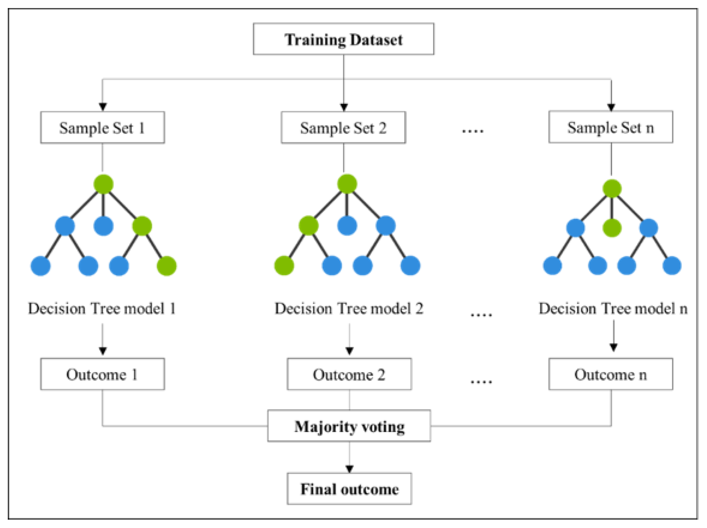
  • Predicting waiting time at mobility restrictions using Random Forest Regression
The Random Forest Regression is a supervised learning algorithm used for regression or classification prediction [53]. The Random Forest algorithm takes a dataset with input features and corresponding labels or outcomes and creates a large number of decision trees, each using a random subset of the data and a random subset of the input features. Each decision tree independently makes a prediction based on its subset of data and features. When a new data point needs to be predicted, it passes through each decision tree and each tree provides its prediction. The final prediction is determined by combining the predictions from all the decision trees, usually through voting or averaging [54]. Figure 2 illustrates the workflow of the Random Forest algorithm.
The RF regression method performs better than other machine learning methods, especially when predicting short-period congestion due to an event that may impact on sustainability [55]. RF Regression is a suitable algorithm for the border crossing time case and for developing a short-term prediction algorithm [56]. Taghipour et al. [49] conducted a short-term travel time prediction algorithm using an Artificial Neural Network, K-Nearest Neighbours, and Random Forest. The results showed that RF presented satisfying results when compared with the other ML models. The randomness in the algorithm helps to prevent overfitting and ensures diversity among the decision trees, leading to more accurate and robust predictions. Also, it has the feature importance technique, using mean decreasing accuracy to evaluate the predictive error and feature significance [52].
Hence, in this study, we incorporated RF regression by using historical records obtained from an extensive field survey to determine the waiting times at different mobility restrictions, which also impact on sustainability. The methodology followed to create the RF waiting time prediction model consisted of the following: (i) data cleaning and preparation; (ii) applying correlation coefficient analysis to identify the input variables (model features)—the vehicle waiting time at the queue, vehicle speed near 750 m of the checkpoint, and day of the week—based on their correlation with the output variable (time to cross the checkpoint); (iii) building the predictive model by splitting the dataset randomly into a training dataset and testing dataset (RF uses the training dataset to build the predictive model, while the testing dataset is used to predict the waiting time); and (iv) evaluating the predicted outcomes and testing the accuracy of the model. Figure 3 illustrates the methodology of creating a waiting time prediction model using RF.

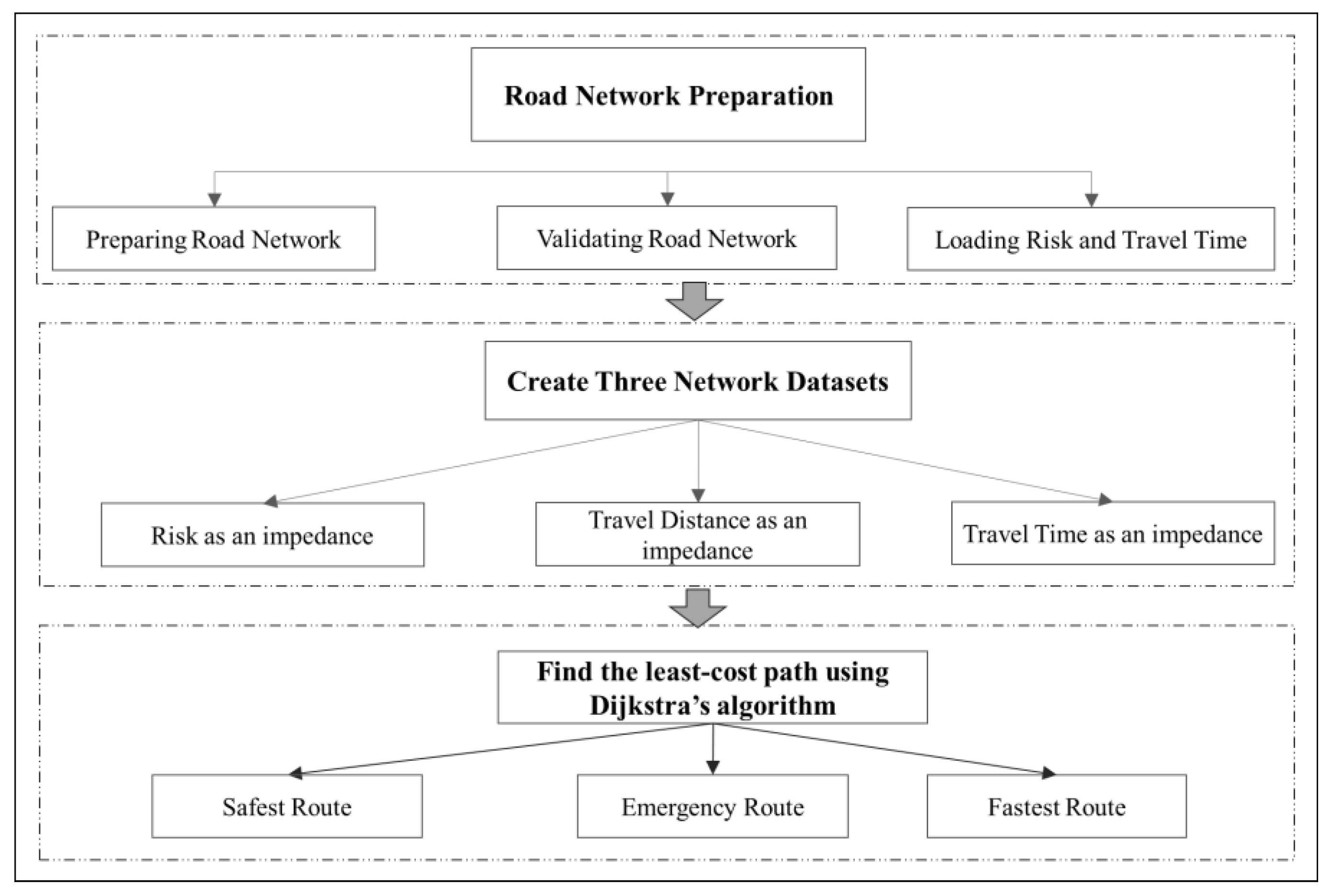
2.2.3. Construction of Route Planning Model

This section describes the methodology of applying the route planning model to find multi-categorised routes (Figure 4).
The first phase includes preparing the road network as a major input in the route planning model. This stage comprises gathering physical and sustainability/environmental data related to the road network, validating its operational and geometric aspects, and integrating cost factors such as risk, time, and distance.
The second phase focuses on network analysis, entailing the creation of three distinct network datasets. Here, three graph models are generated, each associated with a different attribute cost—risk, travel time, and travel distance. This step serves as a preliminary stage for the application of routing analysis algorithms. In the final phase, Dijkstra’s algorithm is employed to determine the least-cost path, generating three alternative categories: safest, shortest, and fastest.
  • Road network preparation
This phase focuses on gathering both historical and real-time data related to the road network. These data encompass details about road segments, road conditions, road classifications, speed limits, permanent mobility restrictions, and prohibited roads. These data can be procured from governmental authorities, non-governmental organisations (NGOs), and crowdsourcing platforms (SRMS).
  • Road network validation
This phase comprises two steps: (i) Identifying the permanently prohibited roads and inaccessibility due to permanent blockades and prohibition policies. These roads will be excluded from the route planning model to enhance the accessibility and usability of the road networks. (ii) Utilising network topology to ensure the connectivity of the network elements, which include nodes and edges essential for the route planning model [57]. Network topology serves as a fundamental quality assurance technique [58] which is used to identify and rectify errors within network connections. These errors may include dangling edges, overlapping edges, and inaccuracies within the road network.
  • Loading cost factors: risk, travel time, and distance
Once the road network has been verified, the road segments are assigned cost factors based on the evaluation parameters used in the route planning model. These parameters include the following: (i) comprehensive risk score (Ri), (ii) weighted travel time (AW), and (iii) length of the road section (Dist). Each of these parameters (Ri, AW, Dist) is treated as an impedance which quantifies the cost associated with traversing a network path or moving from one network element to another [59]. Higher impedance values represent higher costs for movement, and the optimal path in a network is the path with the lowest impedance, often referred to as the least-cost path.
For example, Ri serves as the impedance in determining the safest route, which corresponds to the path with the lowest risk and cost. Dist is the impedance to identifying the shortest route, which corresponds to the path with the shortest travel distance (e.g., an emergency route). AW serves as the impedance for finding the fastest route, representing the path with the lowest travel time cost.
  • Building the graph model and applying route analysis using Dijkstra’s algorithm
The research methodology was applied to the road graph represented by G = (V, E), where V is the set of nodes and E is the set of edges. This step includes assigning the attribute cost (impedance) for each edge of the graph. However, three network datasets will be created to provide the three categories of alternatives (safest, shortest, and fastest); each network has risk, distance, and travel time costs.
The Dijkstra algorithm is an algorithm widely used for finding the shortest path from the origin to all other nodes on a weighted graph, thus impacting on sustainability [60]. Different algorithms have been proposed since Dijkstra’s algorithm was first described, including A* [61], D* [62], D* Lite [63], and ant colony optimisation (ACO) [64]. Dijkstra’s algorithm remains an efficient and effective algorithm for reducing the computational time and power needed to find the shortest path [65]. Our decision to choose Dijkstra’s algorithm is justified by its reputation as the most relevant and widely used algorithm for this purpose and its deterministic method, which can provide reliable results in a fully observed environment [21]. It is also suitable for simple route planning objectives such as safety, travel time, and distance, thus impacting on sustainability.
Dijkstra’s algorithm can be adapted to calculate costs beyond the mere length of each route [66]. In this study, many factors were considered, including not only the cost associated with edge length but also the integrated factors of risk and travel time. Additionally, recent adjustments to the algorithm have been made, enhancing its performance and enabling customisation to adhere to user-defined criteria, including handling one-way restrictions, constraints, and barriers [67], aligning with the objectives of this study.
To find the least-cost path from a starting location, s, to a destination location, t, Dijkstra’s algorithm maintains a set of nodes, V, whose final cost path from s has already been computed. The algorithm repeatedly finds a junction in the set of junctions with the least-cost path estimate, adds it to the set of junctions V, and updates the least-cost path estimates of all neighbours of this junction not in V. The algorithm continues until the destination junction is added to V [68].

3. Results and Discussion
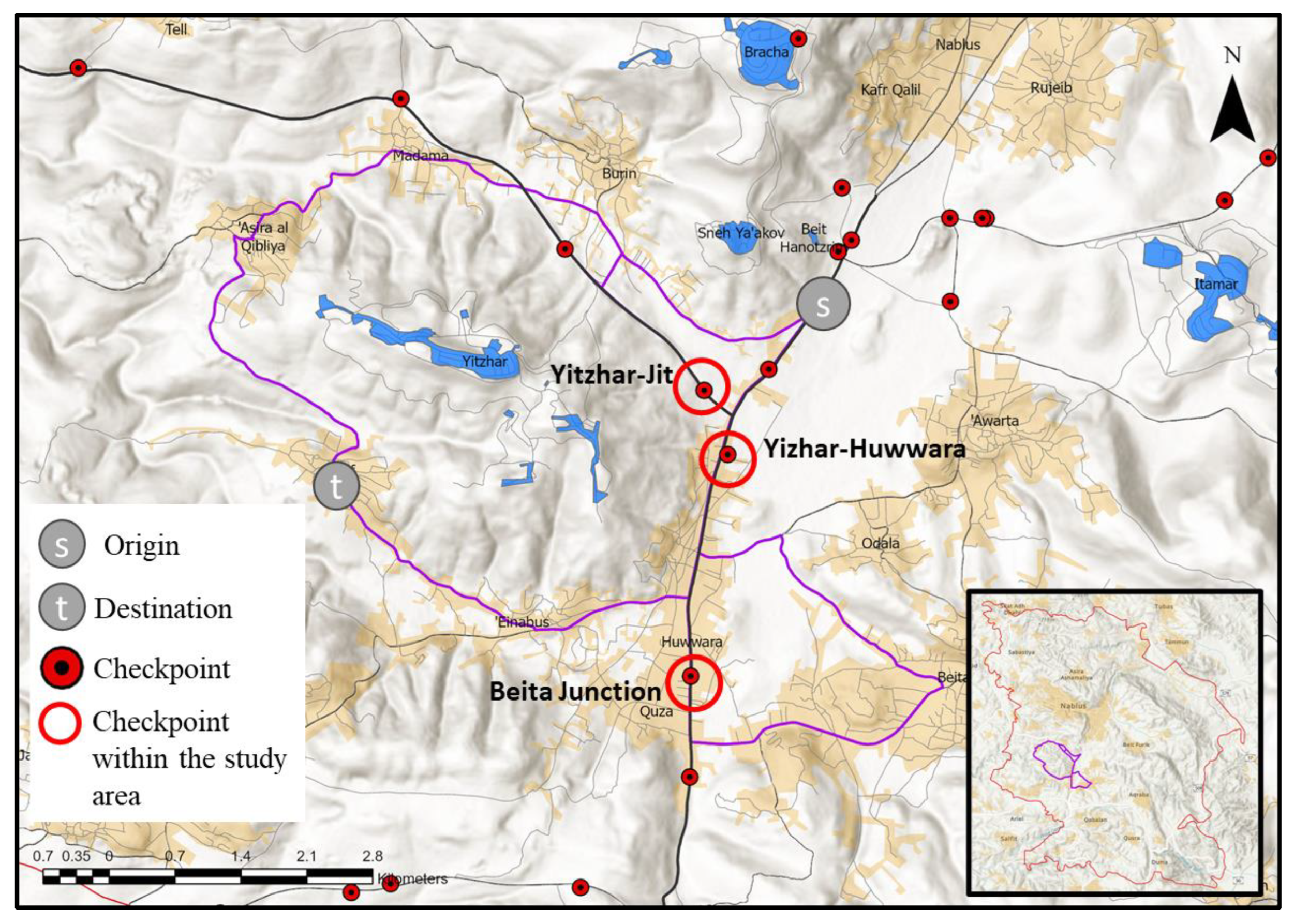
3.1. The Study Area

The research methodology was applied to a road network located in the southwestern part of Nablus Governorate (Figure 5). This part of the road network has a high risk rate, presented in the risk of settler-related violent incidents and mobility restrictions. According to the OCHA report [5], the Nablus Governorate witnessed the highest rate of settler-related violent incidents against Palestinian civilians. From 2021 to early 2023, around 30% of Palestinian fatalities in the Nablus Governorate derived from settler-related incidents. The severity of this risk became more significant with the heavy traffic volume [69], since it includes part of Road 60, a main road connecting the north of the WB with the south (black line in Figure 5).
Besides the risk of settler-related violence, this area is exposed to risk-related mobility restrictions related to three checkpoints (Yitzhar–Huwara, Yitzhar–Jit, and Beita Junction), as illustrated in Figure 5. Also, the study area is exposed to various movement restrictions, such as flying checkpoints, road gates, roadblocks, and earth mounds. So, this part of the road is a good representative sample to study in terms of mobility along the road network in the WB.
The road sample was converted into a graph model G = (V, E), where V is the set of nodes and E is the set of edges. The graph model was created using the capabilities of ArcGIS Pro 3.1. The graph comprises 16 edges (a1, a2, a3, a4…, a16) and 13 nodes (v1, v2, v3, v4…, v13), as illustrated in Figure 6.

3.2. Data Sources and Collection

The road network data were provided by the Palestinian Ministry of Transportation (MOT) in the shapefile format. Mobility restrictions, including permanent checkpoints, road gates, and prohibited road segments, were obtained from the Ministry of Local Government (MOLG) in the shapefile format. Real-time data on mobility restrictions, encompassing checkpoints, road gates, incidents of settler violence, and traffic congestion, were procured from the SRMS platform in the form of web feature layers.
The waiting time data at the mobility restrictions was collected from the Arij Institute (Applied Research Institute–Jerusalem), which tracked 70 vehicles for six months (January–July 2018) on major routes in the West Bank with checkpoints and barriers [70]. More than 18.5 million records were registered and stored in a Microsoft SQL database. Due to the massive amount of data, the institute faced difficulties in retrieving the data from the server for the researchers. However, detailed CSV files for March and June were provided, containing 41,604 GPS records; each row presents the GPS record, and the columns are the captured data, including vehicle location (x,y), average speed within 750 m from the checkpoint, the creation date, the average number of vehicles in the queue, the average waiting time in the queue, and total waiting time (Figure 7).
Information related to historical incidents of settler violence was obtained from the B’tselem Institute (The Israeli Information Center for Human Rights in the Occupied Territories) in the form of text data. Table 3 outlines the essential data required and their respective sources for the application of the route planning service.

3.3. Data Processing and Analysis

This section describes the application of the three-step methodology previously presented in Section 2.2; this methodology was used to construct multi-categorised routes.

3.3.1. Identifying the Comprehensive Risk Score

This phase includes implementing the methodology for determining the comprehensive risk score, as outlined in Section 2.2. Each phase is summarised below:
  • Creating Risk Indicators
The evaluation criteria for calculating Ri includes (i) mobility restrictions, (ii) settler-related violence, (iii) the built environment, and (iv) the physical characteristics of the road edges. These criteria were identified for each road section using the collected data. Table 4 describes the proportion of each index value on the graph model.
Around 37.5% of the edges have mobility restrictions. Violent incidents occurred in an equal ratio in the daytime and nighttime. However, around 67% of the violent incidents occurred during a weekday, and 33.3% occurred during a weekend. The variation in the violent incident rate during the week could be interpreted by the change in the daily average traffic volume, which, according to the data for the year 2020, reached 27.2 thousand on a weekday and 15.2 thousand on a weekend on a section of Road 60 which intersects with the study area [71].
The general physical characteristics of the edges present acceptable conditions; half of the road edges have moderate status, 67% of the edges are lightened, and around 69% of the road edges are located in urban areas and pass near the built-up Palestinian urban areas.
  • Index weight calculation
The pre-identified indices were used to determine the comprehensive risk score Ri. However, these identified risk indices have different weights on the risk level Ri, so EWM was applied using Equations (2)–(7). Table 5 shows that the indicator of NO_VIO (number of previous violence) has the smallest entropy and the largest weight. Therefore, the road edges that witnessed settler-related violent incidents will significantly impact the road risk. In contrast, the indicators of road physical conditions have the lowest weights.
  • Determination of a comprehensive risk score (Ri)
After determining the weight of each index, Equation (1) was applied to calculate the Ri for each road edge, as illustrated in Table 6.

3.3.2. Travel Time

This section pertains to determining the weighted travel time (AW) along the road edges of the study area (n1, n16) using Equation (9). Dist and S data are already known based on the MOT database. However, the predicted waiting time (Tw) is determined by applying the RF prediction model methodology. The waiting time prediction model was applied for each mobility restriction in the study area separately to enhance the accuracy of the prediction results. This included applying the RF prediction model to the Yitzhar–Huwara checkpoint. This methodology could be applied to the other two checkpoints on the road sample under study: Yitzhar–Jit and Beita Junction.
The dataset of the Yizhar–Huwara checkpoint has 2275 records, including the waiting time in the queue in minutes (Time_queue), the average speed within 750 m distance from the Yitzhar–Huwara checkpoint (km per hour), the total waiting time in minutes to cross the Yitzhar–Huwara checkpoint (Time), and the day of the week (DOW). Table 7 provides the descriptive statistics of the numerical variables of the dataset. The total waiting time to cross the checkpoint Tw is the output variable that the machine learning model was trained to predict. The dataset has a mean waiting time value to cross the Yitzhar–Huwara checkpoint of 1.8, a median of 1.6, and a standard deviation of 1 min.
The Random Forest Regression applied the waiting time prediction model using Python 3.9.13 and the Scikit-learn software 1.0.2 library, which contains various classification, clustering, and regression algorithms [56]. The developed code can be found via a GitHub repository [72]. This prediction model incorporates several variables, including waiting time in the queue, vehicle speed, and the day of the week (DOW). Real-time data on traffic flow can significantly influence waiting time predictions [56]. However, due to the unavailability of real-time data regarding traffic flow, the initial step involved constructing the prediction model using historical data.
To avoid overfitting or reduced model performance caused by including numerous variables, a correlation coefficient analysis was performed [73]. Table 8 shows the correlation between the waiting time and other variables. The time the vehicle spends in the queue has a high positive correlation with the waiting time to cross the checkpoint, and the vehicle speed has a strong negative correlation with the waiting time. Such relationships are also linked to sustainability issues. The day of the week variable has a very weak correlation with the waiting time, so it was not used to train the model.
The RF Regression model was created by identifying the time in the queue and vehicle speed as model features. The dataset was split into a training set (80%) and a testing set (20%) to evaluate the model’s performance. The waiting time of the Yitzhar–Huwara checkpoint has a training dataset of 1820 records and a testing dataset of 455 records. The model was created using default Scikit Learn 100 decision trees (estimators) and 42 random states [74]. Scatter plots (Figure 8) were created to compare the tested and predicted values. They presented a linear pattern, indicating convergent values between the predicted and actual data, as illustrated in Figure 8.
The Mean Squared Error (MSE) and R-squared (R2) were used to evaluate the model’s performance. The results show an MSE of 0.25, which indicates that the model’s predictions are quite close to the actual values. The R2 score measures the proportion of the variance in the dependent variable (waiting time) that is predictable from the independent variables (speed and time queue). The results show that R2 is 0.80, which means that about 80% of the variance in the waiting time can be explained by the model. These metrics provide a good indication that the developed prediction model has successfully predicted and explained the waiting time at the checkpoint.
To understand the variables’ contribution towards the model accuracy, the Scikit Learn library provides the features’ relevance. We found that the speed of the vehicles in the queue has a higher relevance in predicting the waiting time, as illustrated in Figure 8. The results of our analysis indicate that if the model was recreated and vehicle speed was the only parameter considered, a higher accuracy could be achieved. This is because vehicle speed is a strong indicator of traffic flow and congestion, and it can be easily captured or measured from various sources like GPS sensors on drivers’ mobile devices.
Figure 8 presents the application of the RF waiting time prediction model on the Yitzhar–Huwara, Beita junction, and Yitzhar–Jit checkpoints, which show good performance, as 92% and 83% of the variance in the waiting time at Beita junction and Yitzhar–Jit can be explained by the model, respectively.

3.3.3. Construction of the Route Planning Model

The route planning model was used to find multi-categorised routes according to the following steps: (i) preparing the road network study area using ArcGIS Pro 3.1; (ii) filtering the road network by removing the prohibited road, which is the road where Palestinian drivers are forbidden to travel, including settlement roads and roads located behind the separation wall [70]; (iii) validating the prepared road network using the network topology technique provided by the ArcGIS Network Analyst (NA) module [21]; (iv) loading Ri, travel time, and distance parameters to the graph edges; and (v) applying Dijkstra’s algorithm to find the route with the lowest level of risk, lowest travel time, and shortest route distance. Figure 9 illustrates the Ri values for each edge of the graph model.
The application of the route planning model was carried out considering a scenario of a vehicle queue near the Yitzhar–Huwara checkpoint with an average speed limit of 10 km/h. Additionally, there was a risk of settler-related violence near the Yitzhar–Huwara checkpoint which was reported in real-time using the SRMS platform, as illustrated in Figure 10.
Considering the proposed scenario, the waiting time at the Yizhar–Huwara checkpoint was forecasted to be 9.5 min. Subsequently, the travel time for each edge was loaded in accordance with Equation (9), as depicted in Figure 11. After loading the risk, travel time, and distance values onto the graph edges, Dijkstra’s algorithm was applied between the starting point s and ending point t to find the three categorised routes. Figure 11 presents the results of the NA analysis.
The observed routes were categorised and are presented in Table 9. It is worth noting that the emergency route exhibits the shortest distances, making it the most efficient in terms of distance. On the other hand, the safest route is characterised by having minimal risk factors, ensuring a secure journey. Meanwhile, the fastest route boasts the lowest travel time, allowing one to quickly arrive at the destination, along with reduced sustainability impacts.

4. Conclusions

This paper has presented a route planning model that emphasises enhancing safety and optimising travel time in areas subjected to mobility restrictions. The research methodology employed a quantitative analysis to calculate a comprehensive risk score; the risk indicators were weighted using the Entropy Weight Method (EWM). These indicators encompassed factors such as the severity of the violent incidents, the number of mobility restrictions, physical road conditions, lighting, and proximity to built-up areas. This study involved calculating travel time by considering the predicted waiting time at the mobility restrictions using Random Forest Regression. To offer travellers a choice of routes that align with their priorities, including sustainability-related ones, the study utilised Dijkstra’s algorithm to find the optimal categorised routes. These routes included the safest route, the fastest route, and the shortest route.
This methodology was applied to a road network located in the southwestern part of Nablus Governorate, which is subjected to high levels of settler-related violence and mobility constraints. The results of the EWM revealed that violent incidents have the highest weight on the comprehensive risk score, while the physical road conditions have the lowest weight. The Random Forest Regression model was applied to three checkpoints distributed along the road network in the study area. The results were promising, with R-squared (R2) values ranging from 80% to 92%.
The route planning model employed Dijkstra’s algorithm to determine categorised routes, providing satisfactory results in terms of analysis complexity and efficiency. However, when dealing with large-scale applications under dynamic changes in mobility restrictions, the use of this algorithm becomes inefficient. It leads to slow and inefficient analysis due to its limited capacity to handle real-time changes. Furthermore, limitations arise from the scarcity of traffic data regarding historical travel times, real-time traffic updates such as accidents, congestion data derived from GPS, weather conditions, and temporal traffic distribution (like day of the week, time of day, etc.). These data sources could significantly enhance the quality of travel time prediction and result analyses. Moreover, further sources of data usable for such applications could be obtained through the installation of totems, cameras, and similar devices, as well as drones flying at peak-hours or on demand (i.e., upon request in case of emergency situations). When possible, such devices could be endowed with automated licence plate recognition features and connected to specific databases that could further enhance the efficiency of safety controls regarding vehicles for each path. These features make the solution proposed in this paper more generally applicable to other contexts, where conflicts, terrorism, sustainability issues, and also other emergency situations (e.g., those related to epidemic restrictions or natural disasters) may exist, considering minor algorithmic adaptations. In this context, many territories could be considered to be among the most adequate examples for applying the principles of this research study (e.g., the conflicts in Ethiopia (Tigray), Mali, Niger, Sudan, and other African areas; the conflicts in Ukraine, Afghanistan, Yemen, and Syria; the recent earthquakes in Turkey and China; and the floods in Libya).
Additionally, a limitation of this study is the absence of a comparative analysis between the regression technique and routing algorithms used in this methodology and earlier state-of-the-art methods. Future studies could consider evaluating the performance of the RF regression model with other sophisticated machine learning methods, such as Artificial Neural Network models, to identify the most effective approach for traffic prediction and disruption analysis. Also, the efficiency of Dijkstra’s algorithm could be compared with alternative heuristic algorithms like A* or real-time awareness algorithms such as Dynamic Programming-based (DP) algorithms. This could enable the handling of real-time changes by continuously updating path costs based on new information. Introducing considerations related to historical travel time and real-time traffic data could further improve the accuracy of travel time predictions.
Furthermore, there is potential in developing integrated systems that not only consider technical aspects but also incorporate user feedback and preferences to create more user-centric and responsive traffic management solutions.

Author Contributions

Conceptualisation, H.A. and I.S.; methodology, H.A. and I.S.; software, H.A.; formal analysis, H.A.; investigation, H.A.; writing—original draft preparation, H.A. and C.G.; writing—review and editing, H.A., I.S. and C.G.; visualisation, H.A.; supervision, I.S.; resources, H.A., I.S. and C.G.; validation, H.A., I.S. and C.G.; data curation, H.A., I.S. and C.G.; funding acquisition, C.G.; project administration, H.A., I.S. and C.G. All authors have read and agreed to the published version of the manuscript.

Funding

This research received no external funding.

Institutional Review Board Statement

Not applicable.

Informed Consent Statement

Not applicable.

Data Availability Statement

The data used in this research are presented in this paper.

Conflicts of Interest

The authors declare no conflicts of interest.

References

  1. Habbas, W.; Berda, Y. Colonial Management as a Social Field: The Palestinian Remaking of Israel’s System of Spatial Control. Curr. Sociol. 2021, 71, 848–865. [Google Scholar] [CrossRef]
  2. Griffiths, M.; Repo, J. Women and Checkpoints in Palestine. Secur. Dialogue 2021, 52, 249–265. [Google Scholar] [CrossRef]
  3. Abrahams, A.S. Hard Traveling: Unemployment and Road Infrastructure in the Shadow of Political Conflict. Political Sci. Res. Methods 2021, 10, 545–566. [Google Scholar] [CrossRef]
  4. Aburas, H.; Shahrour, I. Impact of the Mobility Restrictions in the Palestinian Territory on the Population and the Environment. Sustainability 2021, 13, 13457. [Google Scholar] [CrossRef]
  5. OCHA Data on Casualties. Available online: https://www.ochaopt.org/data/casualties (accessed on 13 February 2023).
  6. B’Tselem Settler Violence in the WB. Available online: https://www.btselem.org/settler_violence_updates_list?f%5B2%5D=nf_district%3A181&f%5B3%5D=nf_type%3A173&f%5B4%5D=date%3A%28min%3A1640995200%2Cmax%3A1672444800%29&page=1 (accessed on 22 January 2023).
  7. UNHRC UN Experts Alarmed by Rise in Settler Violence in Occupied Palestinian Territory. Available online: https://www.ohchr.org/en/press-releases/2021/11/un-experts-alarmed-rise-settler-violence-occupied-palestinian-territory (accessed on 14 March 2023).
  8. Sarraf, R.; McGuire, M.P. Integration and Comparison of Multi-Criteria Decision Making Methods in Safe Route Planner. Expert Syst. Appl. 2020, 154, 113399. [Google Scholar] [CrossRef]
  9. Liao, X.; Zhou, T.; Wang, X.; Dai, R.; Chen, X.; Zhu, X. Driver Route Planning Method Based on Accident Risk Cost Prediction. J. Adv. Transp. 2022, 2022, 5023052. [Google Scholar] [CrossRef]
  10. Lozano Domínguez, J.M.; Mateo Sanguino, T.d.J. Walking Secure: Safe Routing Planning Algorithm and Pedestrian’s Crossing Intention Detector Based on Fuzzy Logic App. Sensors 2021, 21, 529. [Google Scholar] [CrossRef]
  11. Noureddine, M.; Ristic, M. Route Planning for Hazardous Materials Transportation: Multi-Criteria Decision-Making Approach. Decis. Mak. Appl. Manag. Eng. 2019, 2, 66–85. [Google Scholar] [CrossRef]
  12. Zandieh, F.; Ghannadpour, S.F. A Comprehensive Risk Assessment View on Interval Type-2 Fuzzy Controller for a Time-Dependent HazMat Routing Problem. Eur. J. Oper. Res. 2023, 305, 685–707. [Google Scholar] [CrossRef]
  13. Subotić, M.; Stepanović, N.; Tubić, V.; Softić, E.; Bouraima, M.B. Models of Analysis of Credible Deviation from Speed Limits on Two-Lane Roads of Bosnia and Herzegovina. Complexity 2022, 2022, 2832175. [Google Scholar] [CrossRef]
  14. Wachtel, G.; Schmöcker, J.D.; Hadas, Y.; Gao, Y.; Nahum, O.E.; Ben-Moshe, B. Planning for Tourist Urban Evacuation Routes: A Framework for Improving the Data Collection and Evacuation Processes. Environ. Plan B Urban Anal. City Sci. 2021, 48, 1108–1125. [Google Scholar] [CrossRef]
  15. Ikeda, Y.; Inoue, M. An Evacuation Route Planning for Safety Route Guidance System after Natural Disaster Using Multi-Objective Genetic Algorithm. Procedia Comput. Sci. 2016, 96, 1323–1331. [Google Scholar] [CrossRef]
  16. Ceccato, V.; Gaudelet, N.; Graf, G. Crime and Safety in Transit Environments: A Systematic Review of the English and the French Literature, 1970–2020; Springer: Berlin/Heidelberg, Germany, 2022; Volume 14, ISBN 0123456789. [Google Scholar]
  17. Aytac, M. Work-Related Violence and Stress: The Case of Taxi Drivers in Turkey. Financ. Manag. Sci. 2017, 3, 1–9. [Google Scholar]
  18. Mayhew, C.; Graycar, A. Violent Assaults on Taxi Drivers: Incidence Patterns and Risk Factors. Trends Issues Crime Crim. Justice Ser. 2000, 178, 1–6. [Google Scholar]
  19. Statista Number of Crime Events in the Public Transportation Systems in the United States in 2019. Available online: https://www.statista.com/statistics/1295845/number-crime-events-public-transit-us-by-type/ (accessed on 2 February 2023).
  20. Alpkoçak, A.; Cetin, A. Safe Map Routing Using Heuristic Algorithm Based on Regional Crime Rates. Lect. Notes Data Eng. Commun. Technol. 2020, 43, 335–346. [Google Scholar] [CrossRef]
  21. Peng, N.; Xi, Y.; Rao, J.; Ma, X.; Ren, F. Urban Multiple Route Planning Model Using Dynamic Programming in Reinforcement Learning. IEEE Trans. Intell. Transp. Syst. 2022, 23, 8037–8047. [Google Scholar] [CrossRef]
  22. Aburas, H. SRMS Paltform. Available online: https://experience.arcgis.com/experience/6f33d774efb74ed497bb79daac78a1de/page/Page/?fbclid=IwAR2sjH2MO0jRDQQOyY-p0zv7LQ-HZThQ1_9yOXrS18cej-tRzfTSwz75hW8 (accessed on 6 October 2023).
  23. Agrawal, S.; Gupta, R.D. Web GIS and Its Architecture: A Review. Arab. J. Geosci. 2017. [Google Scholar] [CrossRef]
  24. Esri Shapefile. Available online: https://doc.arcgis.com/en/arcgis-online/reference/shapefiles.htm#:~:text=AshapefileisanEsri,andcontainsonefeatureclass. (accessed on 7 April 2023).
  25. Borker, G. Safety First: Perceived Risk of Street Harassment and Educational Choices of Women; Working Paper; World Bank: Washington, DC, USA, 2021. [Google Scholar]
  26. Richardson, S.; Windau, J. Fatal and Nonfatal Assaults in the Workplace, 1996 to 2000. Clin. Occup. Environ. Med. 2003, 3, 673–689. [Google Scholar] [CrossRef]
  27. Balcells, L.; Stanton, J.A. Violence against Civilians during Armed Conflict: Moving beyond the Macro- and Micro-Level Divide. Annu. Rev. Political Sci. 2021, 24, 45–69. [Google Scholar] [CrossRef]
  28. Couto, M.; Lawoko, S.; Svanström, L. Violence Against Drivers and Conductors in the Road Passenger Transport Sector in Maputo, Mozambique. Afr. Saf. Promot. A J. Inj. Violence Prev. 2011, 7, 17–36. [Google Scholar] [CrossRef]
  29. Essenberg, B. SECTORAL ACTIVITIES PROGRAMME Working Paper Violence and Stress at Work in the Transport Sector. 2003. Available online: https://ideas.repec.org/p/ilo/ilowps/993631343402676.html (accessed on 22 April 2023).
  30. Dunckel Graglia, A. Finding Mobility: Women Negotiating Fear and Violence in Mexico City’s Public Transit System. Gend. Place Cult. 2016, 23, 624–640. [Google Scholar] [CrossRef]
  31. Ding, X.; Chong, X.; Bao, Z.; Xue, Y.; Zhang, S. Fuzzy Comprehensive Assessment Method Based on the Entropy Weight Method and Its Application in the Water Environmental Safety Evaluation of the Heshangshan Drinking Water Source Area, Three Gorges Reservoir Area, China. Water 2017, 9, 329. [Google Scholar] [CrossRef]
  32. Zhu, Y.; Tian, D.; Yan, F. Effectiveness of Entropy Weight Method in Decision-Making. Math. Probl. Eng. 2020, 2020, 3564835. [Google Scholar] [CrossRef]
  33. Stević, Ž.; Subotić, M.; Softić, E.; Božić, B. Multi-Criteria Decision-Making Model for Evaluating Safety of Road Sections. J. Intell. Manag. Decis. 2022, 1, 78–87. [Google Scholar] [CrossRef]
  34. Yannis, G.; Kopsacheili, A.; Dragomanovits, A.; Petraki, V. State-of-the-Art Review on Multi-Criteria Decision-Making in the Transport Sector. J. Traffic Transp. Eng. (Engl. Ed.) 2020, 7, 413–431. [Google Scholar] [CrossRef]
  35. Farooq, D.; Moslem, S.; Jamal, A.; Butt, F.M.; Almarhabi, Y.; Tufail, R.F.; Almoshaogeh, M. Assessment of Significant Factors Affecting Frequent Lane-Changing Related to Road Safety: An Integrated Approach of the Ahp–Bwm Model. Int. J. Environ. Res. Public Health 2021, 18, 628. [Google Scholar] [CrossRef]
  36. Xiao, M.; Luo, R.; Yu, X.; Chen, Y. Comprehensive Ranking of Road Safety Condition by Using the Functional and Material Performance Index. Constr. Build. Mater 2022, 324, 126644. [Google Scholar] [CrossRef]
  37. Sun, J.; Liu, S.; Wang, L.; He, Z. Safety Resilience Evaluation of Urban Public Bus Based on Comprehensive Weighting Method and Fuzzy Comprehensive Evaluation Method. In Proceedings of the 2020 International Conference on Urban Engineering and Management Science, Zhuhai, China, 24–26 April 2020; pp. 370–379. [Google Scholar] [CrossRef]
  38. Wu, R.M.X.; Zhang, Z.; Yan, W.; Fan, J.; Gou, J.; Liu, B.; Gide, E.; Soar, J.; Shen, B.; Fazal-E-Hasan, S.; et al. A Comparative Analysis of the Principal Component Analysis and Entropy Weight Methods to Establish the Indexing Measurement. PLoS ONE 2022, 17, e0262261. [Google Scholar] [CrossRef]
  39. Cai, X.; Lei, C.; Peng, B.; Tang, X.; Gao, Z. Road Traffic Safety Risk Estimation Method Based on Vehicle Onboard Diagnostic Data. J. Adv. Transp. 2020, 2020, 3024101. [Google Scholar] [CrossRef]
  40. Du, W.; Ding, S. A Survey on Multi-Agent Deep Reinforcement Learning: From the Perspective of Challenges and Applications. Artif. Intell. Rev. 2021, 54, 3215–3238. [Google Scholar] [CrossRef]
  41. Yao, Y.; Peng, Z.; Xiao, B. Parallel Hyper-Heuristic Algorithm for Multi-Objective Route Planning in a Smart City. IEEE Trans. Veh. Technol. 2018, 67, 10307–10318. [Google Scholar] [CrossRef]
  42. Wang, H.; Tang, X.; Kuo, Y.H.; Kifer, D.; Li, Z. A Simple Baseline for Travel Time Estimation Using Large-Scale Trip Data. ACM Trans. Intell. Syst. Technol. 2019, 10, 1–22. [Google Scholar] [CrossRef]
  43. Laoide-Kemp, D.; O’Mahony, M. Dealing with Latency Effects in Travel Time Prediction on Motorways. Transp. Eng. 2020, 2, 100009. [Google Scholar] [CrossRef]
  44. Prokhorchuk, A.; Dauwels, J.; Jaillet, P. Estimating Travel Time Distributions by Bayesian Network Inference. IEEE Trans. Intell. Transp. Syst. 2020, 21, 1867–1876. [Google Scholar] [CrossRef]
  45. Serin, F.; Alisan, Y.; Kece, A. Hybrid Time Series Forecasting Methods for Travel Time Prediction. Phys. A Stat. Mech. Its Appl. 2021, 579, 126134. [Google Scholar] [CrossRef]
  46. Mokhtarimousavi, S.; Anderson, J.C.; Azizinamini, A.; Hadi, M. Factors Affecting Injury Severity in Vehicle-Pedestrian Crashes: A Day-of-Week Analysis Using Random Parameter Ordered Response Models and Artificial Neural Networks. Int. J. Transp. Sci. Technol. 2020, 9, 100–115. [Google Scholar] [CrossRef]
  47. Zhao, J.; Gao, Y.; Tang, J.; Zhu, L.; Ma, J. Highway Travel Time Prediction Using Sparse Tensor Completion Tactics and K -Nearest Neighbor Pattern Matching Method. J. Adv. Transp. 2018, 2018, 5721058. [Google Scholar] [CrossRef]
  48. Bachu, A.K.; Reddy, K.K.; Vanajakshi, L. Bus Travel Time Prediction Using Support Vector Machines for High Variance Conditions. Transport 2021, 36, 221–234. [Google Scholar] [CrossRef]
  49. Taghipour, H.; Parsa, A.B.; Mohammadian, A. A Dynamic Approach to Predict Travel Time in Real Time Using Data Driven Techniques and Comprehensive Data Sources. Transp. Eng. 2020, 2, 100025. [Google Scholar] [CrossRef]
  50. Kyritsis, A.I.; Deriaz, M. A Machine Learning Approach to Waiting Time Prediction in Queueing Scenarios. In Proceedings of the 2019 Second International Conference on Artificial Intelligence for Industries (AI4I), Laguna Hills, CA, USA, 25–27 September 2019; pp. 17–21. [Google Scholar] [CrossRef]
  51. Curtis, C.; Liu, C.; Bollerman, T.J.; Pianykh, O.S. Machine Learning for Predicting Patient Wait Times and Appointment Delays. J. Am. Coll. Radiol. 2017, 15, 1310–1316. [Google Scholar] [CrossRef]
  52. Sanit-in, Y.; Saikaew, K.R. Prediction of Waiting Time in One-Stop Service. Int. J. Mach. Learn. Comput. 2019, 9, 322–327. [Google Scholar] [CrossRef]
  53. Anand, A.; Patel, R.; Rajeswari, D. A Comprehensive Synchronization by Deriving Fluent Pipeline and Web Scraping through Social Media for Emergency Services. In Proceedings of the 2022 International Conference on Advances in Computing, Communication and Applied Informatics (ACCAI), Chennai, India, 28–29 January 2022. [Google Scholar] [CrossRef]
  54. Sipper, M.; Moore, J.H. Conservation Machine Learning: A Case Study of Random Forests. Sci. Rep. 2021, 11, 3629. [Google Scholar] [CrossRef]
  55. Lin, Y.; Li, R. Real-Time Traffic Accidents Post-Impact Prediction: Based on Crowdsourcing Data. Accid. Anal. Prev. 2020, 145, 105696. [Google Scholar] [CrossRef]
  56. Sharma, S.; Kang, D.H.; Montes de Oca, J.R.; Mudgal, A. Machine Learning Methods for Commercial Vehicle Wait Time Prediction at a Border Crossing. Res. Transp. Econ. 2021, 89, 101034. [Google Scholar] [CrossRef]
  57. Ahmed, S.; Ibrahim, R.F.; Hefny, H.A. GIS-Based Network Analysis for the Roads Network of the Greater Cairo Area. In Proceedings of the International Conference on Applied Research in Computer Science and Engineering ICAR’17, Beirut, Lebanon, 22–23 June 2017; Volume 2144, pp. 1–9. [Google Scholar]
  58. Esri Network Topology. Available online: https://pro.arcgis.com/en/pro-app/latest/help/data/utility-network/about-network-topology.htm (accessed on 22 March 2023).
  59. Esri GIS Dictionalry. Available online: https://support.esri.com/en-us/gis-dictionary/impedance (accessed on 28 January 2023).
  60. Dijkstra, E.W. A Note on Two Problems in Connexion with Graphs. Numer. Mathmatik 1959, 1, 269–271. [Google Scholar] [CrossRef]
  61. Hart, P.E.; Nils, J.; Nilsson, B.R. A Formal Basis for the Heuristic Determination of Minimum Cost Paths. IEEE Trans. Syst. Sci. Cybern. 1968, 4, 100–107. [Google Scholar] [CrossRef]
  62. Stentz, A. Optimal and Efficient Path Planning for Unknown and Dynamic Environments. Int. J. Robot. Autom. 1995, 10, 89–100. [Google Scholar]
  63. Koenig, S.; Likhachev, M. ID* Lite: Improved D* Lite algorithm. AAAI-02 Proc. 2002, 15, 476–483. [Google Scholar] [CrossRef]
  64. Dorigo, M.; Gianni, D.C. Ant Colony Optimization: A New Meta-Heuristic. In Proceedings of the 1999 Congress on Evolutionary Computation-CEC99 (Cat. No. 99TH8406), Washington, DC, USA, 6–9 July 1999; pp. 1470–1477. [Google Scholar]
  65. Karadimas, N.V.; Kolokathi, M.; Defteraiou, G.; Loumos, V. Ant Colony System vs ArcGIS Network Analyst: The Case of Municipal Solid Waste Collection. In Proceedings of the 5th WSEAS International Conference on Environment, Ecosystems and Development, Tenerife, Spain, 14–16 December 2007; pp. 128–134. [Google Scholar] [CrossRef]
  66. Mirahadi, F.; McCabe, B.Y. EvacuSafe: A Real-Time Model for Building Evacuation Based on Dijkstra’s Algorithm. J. Build. Eng. 2021, 34, 101687. [Google Scholar] [CrossRef]
  67. Esri Algorithms Used by Network Analyst. Available online: https://pro.arcgis.com/en/pro-app/latest/help/analysis/networks/algorithms-used-by-network-analyst.htm (accessed on 10 January 2023).
  68. Rachmawati, D.; Gustin, L. Analysis of Dijkstra’s Algorithm and A∗ Algorithm in Shortest Path Problem. J. Phys. Conf. Ser. 2020, 1566, 012061. [Google Scholar] [CrossRef]
  69. Al-Sahili, K.; Dwaikat, M. Modeling Geometric Design Consistency and Road Safety for Two-Lane Rural Highways in the West Bank, Palestine. Arab. J. Sci. Eng. 2019, 44, 4895–4909. [Google Scholar] [CrossRef]
  70. Arij Assessing the Impacts of Israeli Movement Restrictions on the Mobility of People and Goods. 2019. Available online: https://www.arij.org/publications/special-reports/special-reports-2019/assessing-the-impacts-of-israeli-movement-restrictions-on-the-mobility-of-people-and-goods-in-the-west-bank-2019/ (accessed on 7 March 2022).
  71. Statistics, C.B. of Traffic Volume on Judea and Samaria. Available online: https://www.cbs.gov.il/en/Statistics/Pages/Tools-and-Databases.aspx (accessed on 12 April 2022).
  72. Aburas, H. Waiting-Time-Prediction-Using-RF-Model. Available online: https://github.com/hala-aburas/waiting-time-prediction-using-RF-model.git (accessed on 19 June 2023).
  73. Mour, R.; Carvalho, R.; Carvalho, R.; Ramos, G. Predicting Waiting Time Overflow on Bank Teller Queues. In Proceedings of the 2017 16th IEEE International Conference on Machine Learning and Applications (ICMLA), Cancun, Mexico, 18–21 December 2017; pp. 842–847. [Google Scholar] [CrossRef]
  74. Pedregosa, F.; Varoquaux, G.; Gramfort, A.; Michel, V.; Thirion, B. Scikit-Learn: Machine Learning in Python Fabian. J. Ofmachine Learn. Res. 2011, 12, 2825–2830. [Google Scholar] [CrossRef]
Figure 1. Research methodology.
Sustainability 16 00660 g001
Figure 2. The workflow of Random Forest models.
Sustainability 16 00660 g002
Figure 3. Methodology of creating a waiting time prediction model using RF.
Sustainability 16 00660 g003
Figure 4. Methodology of building the route planning model.
Sustainability 16 00660 g004
Figure 5. Route planning application area.
Sustainability 16 00660 g005
Figure 6. Graph model of road sample study.
Sustainability 16 00660 g006
Figure 7. Arij field survey for checkpoint waiting time [70].
Sustainability 16 00660 g007
Figure 8. The RF waiting times at the checkpoints in the study area predicted by the model and the related feature importance ranking.
Sustainability 16 00660 g008
Figure 9. Ri values for each edge of the graph.
Sustainability 16 00660 g009
Figure 10. Illustration of the proposed scenario.
Sustainability 16 00660 g010
Figure 11. Loading travel time values for each edge and the results of applying Dijkstra’s algorithm.
Sustainability 16 00660 g011
Table 1. Descriptions of the data and sources needed to build a route planning model.
DatasetDescriptionSourcesSource TypeData TypeData Format
road networkroad network geometry, attributes, speed limits, andgovernmental authoritiesauthoritative dataspatial datashapefile
physical restrictionspermanent checkpoints, road gates, physical barriersgovernmental authoritiesauthoritative dataspatial datashapefile
real-time restriction types, locations,
waiting times at restrictions
SRMS platform
NGOs
crowdsourcing data
open source
spatial data
tabular data
WFS 1
Excel sheet
violent incident restrictionsthe incident’s location, time of day, and day of the weekNGOsopen-source datatext datatext
the incident’s location and timeSRMS platformcrowdsourcing dataspatial dataWFS
1 Web Feature Service.
Table 2. The evaluation criteria and the derived indexes for evaluating the risk on the road section.
No.IndexDefinitionDescription
1NO_RISTno. of permanent mobility restrictions no. of permanent restrictions = 1, 2, 3, no mobility restriction = 0
2NO_VIOno. of historical violence actions against vehicles no. of violent actions against the drivers = 1, 2, 3, no record = 0
3TODtime of daydaytime = 1, night time = 2
4DOWday of weekweekday = 1, weekend = 2
5LGT_CONlight conditionavailable = 1, not available = 0
6ROAD_CONroadway surface conditionquality of road surface: good = 1, moderate = 2, bad = 3
7ADJ_BUILTUPtype of the adjacent built-up arearural = 1, urban = 2
Table 3. Data required for the application of the route planning service and their sources.
DatasetDescriptionSourcesData Format
road networkroad network geometry, attributes, and speed limits.MOTshapefile
mobility restrictionspermanent checkpoints, road gates, prohibited roads.MOLGshapefile
real-time restriction type and location.SRMS PlatformWFS
waiting time at restrictions.ArijExcel sheet
violence incidents restrictionsincident’s location, time of day, and day of the week.B’Teselemtext
incident’s location and time.SRMS PlatformWFS
Table 4. Descriptive statistics for the evaluation criteria.
No.IndexStatistical Value (Proportion)
1NO_RIST1 = 37.5%, 0 = 62.5%
2NO_VIO1 = 18.6%, 3 = 6.3%, 4 = 6.3%, 5 = 6.3%, 0 = 62.5%
3TOD1 = 50%, 2 = 50%
4DOW1 = 66.7%, 2 = 33.3%
5LGT_CON1 = 56.2%, 0 = 43.8%
6ROAD_CON1 = 3%, 2 = 56.2%, 3 = 18.8%
7ADJ_BUILTUP1 = 31.2%, 2 = 68.8%
Table 5. Weights of the cost risk index.
No.IndexejWj
1NO_RIST0.6460.148
2NO_VIO0.5700.180
3TOD0.6250.157
4DOW0.6250.158
5LGT_CON0.7010.125
6ROAD_CON0.8760.051
7ADJ_BUILTUP0.5800.176
Table 6. Risk values of the graph edges.
Road EdgeNO_RISTNO_VIOTODDOWLGT_CONROAD_CONADJ_BUILTUPRi
a10.000010.000010.000010.000010.00001110.229
a211121111.158
a313211121.696
a410.000010.000010.000011310.607
.
.
.
.
.
.
.
.
.
.
.
.
.
.
.
.
.
.
.
.
.
.
.
.
.
.
.
a140.000010.000010.000010.000011220.583
a150.000010.000010.000010.000011210.406
a1615111211.776
Table 7. Descriptive statistics for the dataset.
TimeSpeedTime_Queue
mean1.851.80.1
std1.014.40.5
min0.30.00.0
50%1.653.00.0
max15.3101.08.2
Table 8. Correlation between waiting time at the checkpoint and the other variables used to develop predictive models.
Correlation CoefficientTime in the QueueVehicle SpeedDOW
Waiting Time at checkpoint0.85−0.74−0.13
Table 9. Costs of categorised observed routes.
Time Cost
(min)
Risk CostLength Cost
(m)
Emergency 10.63.586689
Safest13.51.749412
Fastest13.13.959782
Disclaimer/Publisher’s Note: The statements, opinions and data contained in all publications are solely those of the individual author(s) and contributor(s) and not of MDPI and/or the editor(s). MDPI and/or the editor(s) disclaim responsibility for any injury to people or property resulting from any ideas, methods, instructions or products referred to in the content.

