The Optimization of Bus Departure Time Based on Uncertainty Theory—Taking No. 207 Bus Line of Nanchang City, China, as an Example

Abstract

In order to optimize the bus departure time considering uncertain factors, this paper constructed an uncertain bi-level programming model for departure frequency and scheduling of a bus line. The uncertainty of passenger arrival and bus operation time were taken into account, combined with actual operation conditions. Nanchang 207 bus line was taken as an example to optimize the departure frequency and scheduling in the morning peak hour. The optimal departure frequency in the morning peak hour is 12 times. The overall index value of the route’s non-uniform scheduling during peak hours increased by 0.06 and 9.23% compared with uniform scheduling. The analysis results show that the effect of the non-uniform scheduling is obvious. The issue of bus line departure frequency and scheduling has a positive effect on improving the efficiency of public transportation, reducing operating costs and promoting the sustainable development of the public transportation system. This paper provides a theoretical support for bus operators to optimize route operations.

1. Introduction

With the characteristics of safety, high efficiency, convenience, and environmental protection, public transportation has become an effective transportation mode to alleviate urban transportation problems [1]. It has become a general consensus to prioritize the development of public transportation [2]. The development of regular bus routes and bus vehicle configuration issues are not only related to the costs and benefits of the bus company but also have an essential relationship with the service level of buses and passenger satisfaction [3,4]. The core of bus allocation is the optimization of departure intervals to meet passenger flow demand. Therefore, the optimization of bus departure intervals is of positive significance for the sustainable development of the public transport system. Bus vehicle configuration and bus departure intervals are closely related. Bus vehicle configuration refers to the number and type of vehicles configured on the bus route. The minimum bus departure interval is subject to the number of vehicles configured on the bus route and the bus operation time. How to determine an optimal departure frequency and optimize the social benefits of bus services while ensuring the basic benefits of bus operators is a question worthy of discussion. The bus vehicle configuration of bus lines should meet the departure frequency of the peak period. Therefore, the problem of bus line vehicle allocation is able to be transformed into the problem of optimizing the departure frequency of bus lines during peak hours.

Many scholars have conducted in-depth research on the optimization of bus vehicle configuration and departure intervals. The two-level programming model that considers the benefits of bus operators and passengers has been commonly used. Di Zhen [5] considered the revenue of bus companies as the upper-level objective; the minimum weighted total cost of travel time and cost of passengers was the lower-level objective, and government behavior was used as a constraint to establish a two-level programming model for the bus line vehicle allocation problem. Zhao Shuzhi [6] established a multi-model bus route allocation optimization model based on the weighted sum of bus operator costs and bus service levels. Liu Tao [3] researched public transport timetables and vehicle scheduling problems and developed a bi-objective, bi-level programming model. The upper objective is to minimize the total operating cost and the total travel time of passengers from the perspective of the bus operator. The lower model is for a traffic distribution issue based on the departure time and vehicle capacity constraints. Filipe Monnerat [7] researched fleet management problems and established a vehicle and driver assignment model with an objective function of minimizing the total cost. Liujiang Kang [8] developed three integer linear programming models (ILPM) to describe bus and driver scheduling problems with meantime windows for a single bus line. M.A. Goberna [9] dealt with solutions problems for uncertain multi-objective convex programs, which allowed the data of the objective function and the constraints to be uncertain.

However, uncertainty realizations play an important role in real-world applications [10]. There are many uncertain factors in the operation of public transportation: the service time windows and passenger demand of different stops cannot be accurately estimated. During the development of bus lines and bus vehicle allocations, these variables are typically estimated on the basis of historical data or experience, so that a relatively reliable result is obtained; this will result in large errors. In order to decrease the error, the methods for optimization under uncertain factors have been widely studied over past decades [10]. Real decisions are generally made under the state of indeterminacy [11]. Randomness, grayness, and fuzziness are three inseparable uncertain factors that affect real decisions [12]. There are two mathematical systems for modeling the indeterminacy: one is probability theory [13], and the other is uncertainty theory [11]. Probability is interpreted as frequency, while uncertainty is interpreted as personal belief degree [11]. Frequency is the empirical basis of probability theory, while belief degree is the empirical basis of uncertainty theory. Savage [14] said a rational man behaved as if he used subjective probabilities. In other words, a rational person is expected to hold belief degrees that follow the laws of uncertainty theory rather than probability theory. In order to minimize the error of indeterminacy and unify the descriptions of grayness, randomness, and fuzziness as three inseparable uncertain factors, Liu Baoding [15] put forward the uncertainty theory in 2007 and continuously improved it to form a standardized axiomatic mathematical system. Liu [16] introduced uncertain variables when considering programming problems in 2009 and proposed uncertain programming. Stochastic uncertainty is caused by parameter variations but also from an epistemic uncertainty caused by a lack of knowledge about the system.

The uncertainty theory represented by uncertain programming has been widely and successfully applied in the fields of transportation, logistics, and finance [10,16,17]. The applications of uncertainty theory in transportation problems mainly include vehicle scheduling problems, critical road problems, etc. Jiao Dengya [18] built an uncertain programming model based on Liu Baoding’s research to solve the logistics of the vehicle scheduling problem with uncertain factors, which took into account the uncertainty of the demand for goods and the travel time among the delivery points. A genetic algorithm that can effectively solve the uncertain programming model of vehicle scheduling is designed. Liu Wusheng [19] used the bus IC card data to analyze the passenger flow uncertainty of bus stops and proposed a probabilistic derivation model and algorithm, without applying it to bus vehicle allocation, operation scheduling, and other issues. Wei Ming [20] constructed a bi-level programming model for solving uncertain bus scheduling problems. The constraints such as depot capacities, fueling, and emissions of polluting gases are considered in the bi-level programming model. The genetic algorithm for solving the upper and lower models is designed, the concept of satisfactory solutions is introduced, and a set of satisfactory solutions produced by the lower programming are compared and selected by the upper programming, and then the best bus dispatching plan as well as the corresponding vehicle purchase plan are generated. Lin Chen [21] established uncertain goal programming models for bicriteria solid transportation problems: the transportation cost and time, conveyance capacities, supplies, and demands were regarded as uncertain variables in the model. By applying some properties of uncertainty theory, the chance-constrained goal programming model and the expected value goal programming model can be, respectively, transformed into the corresponding deterministic equivalents [21]. Based on uncertainty theory, Jun Guo [22] proposed a vehicle scheduling method considering the dynamic departure interval and vehicle configuration of electric buses (EBs). An uncertain bi-level programming model (UBPM) was established, which took the total cost of passenger travel (CP) as the upper objective function and the total cost of EBs (CB) as the lower. Bing Zhang [23] established a two-level planning model that takes the maximum total revenue of the bus company as the upper-level goal and the minimum total travel cost of passengers as the lower-level goal and used uncertainty theory to study and design customized bus routes with uncertain factors. Bin Zhan [24] established a bi-level programming model to determine the frequency of the bus vehicles and non-uniform interval optimization considering the uncertainty of passenger demand, without considering the uncertainty of bus travel time.

The vehicle scheduling problem is well known as an NP-hard problem; in order to solve the problem, Lu Sun [25] considered the vehicle scheduling problem with an uncertain processing time and proposed a hybrid cooperative co-evolution algorithm (hccEA). The results prove the efficiency and effectiveness of hccEA, and future research will apply the algorithm on multiple objectives of the uVSP (uncertain vehicle scheduling problem). Hannah Bakker [10] reviewed multi-stage optimization under uncertainty; problems requiring a sequence of decisions considering uncertainty in reality are of crucial relevance in real-world applications, e.g., vehicle scheduling, supply chain planning, or finance. While models for multi-stage optimization under uncertainty have often been addressed from a specific application-driven point of view (pre-determining the style of uncertainty representation and solution methodology), the classification possibilities and insights shown in this review can form the basis of an undistorted and consistent model for the analysis of multi-stage uncertainty problems considering potentials of a variety of uncertainty models, solution methods, and evaluation techniques [10]. Federica Ciccullo [26] developed a method to link supply uncertainty and sustainable supply chain strategies, which has a positive effect on logistics and transportation. However, when sustainability is a desirable attribute or an order winner, companies might implement sustainable practices aiming at reducing supply uncertainty rather than for sustainability goals.

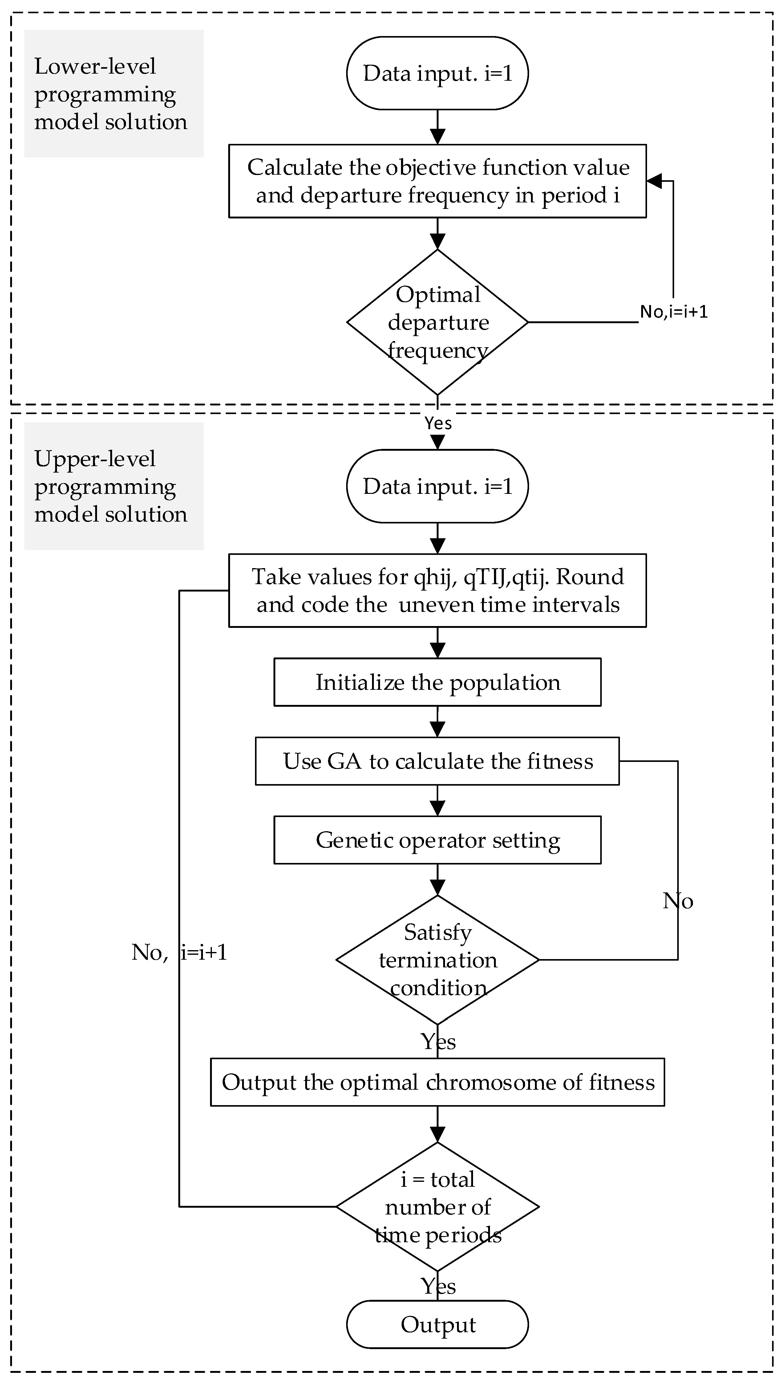
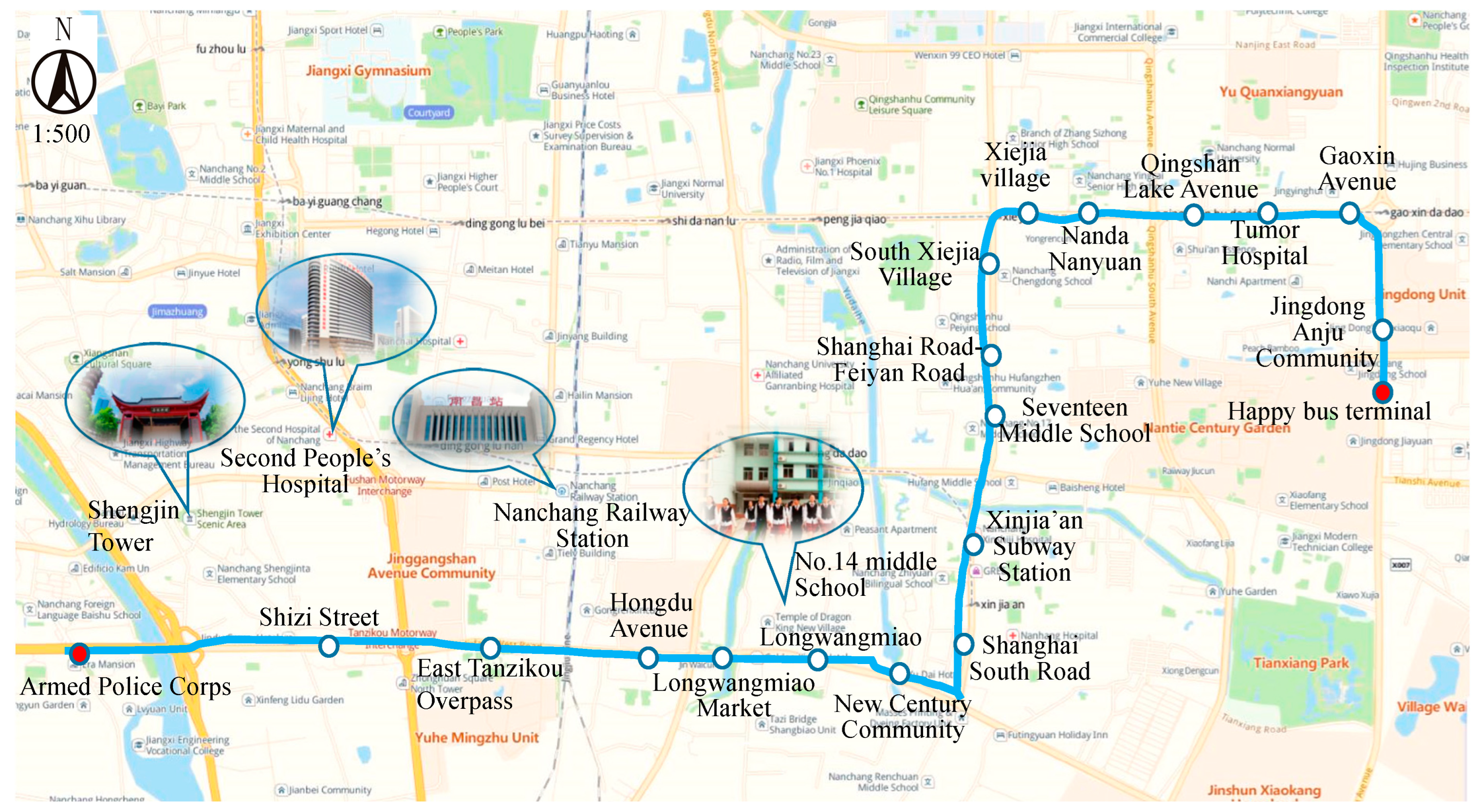
To sum up, although many scholars have conducted in-depth research on the optimization of bus vehicle configuration, and the uncertain theory has been widely and successfully applied in the fields of transportation and logistics, few results have been obtained using the uncertainty theory to study bus vehicle configuration problems. This paper considers the uncertainty of the number of passengers at the bus station and the bus operation time, as well as the cost and benefits of bus operators and bus passengers. An uncertain bi-level programming model is established with a view to providing theoretical support for bus departure time problems. The structure of the thesis is to briefly introduce the uncertainty theory, then build an uncertain bi-level programming model for the bus departure time problem, and design a solution algorithm. No. 207 bus line of Nanchang city, China, is taken as an example for case analysis, and the last section is the research conclusion.

2. Uncertainty Theory

The number of passengers arriving at each bus station over a period of time (such as a departure interval) and the operating time between bus stops are uncertain. The number of travelers arriving at each station fluctuates within a range, which is an uncertain variable. Since the number of passengers at bus stops and the running time between bus stops are uncertain variables, their uncertain distributions are the key to the research problem. The concepts of uncertain variable and uncertain distribution are supposed to be given in the description of the methodology. Objectively speaking, uncertainty measure and uncertainty space are the basis of uncertainty variables and uncertainty distribution. Therefore, the descriptions of the above concepts are necessary, and the related concepts of uncertainty theory are given in Section 2.1 and Section 2.2 based on [15]. The index of symbols used in this section is listed in

Table 1. The index of symbols used in Section 2.

Symbol	Description
L	a $\sigma -$ algebra on a non-empty set $\mathsf{\Gamma }$
$\mathsf{\Gamma }$	a non-empty set
$\mathsf{{\rm M}}:L\to [0,1]$	set function from L to interval [0.1]
$\mathsf{\Lambda }$	an event
${\mathsf{\Lambda }}^C$	the complement of $\mathsf{\Lambda }$;
$(\mathsf{\Gamma },L,\mathsf{{\rm M}})$	uncertainty space, composed of $\mathsf{\Gamma }$, L and the uncertainty measure M
$\Re$	the real number set
$\xi$	an uncertain variable, it is a measurable function from the uncertain space $(\mathsf{\Gamma },L,\mathsf{{\rm M}})$ to the real number set $\Re$
$B$	any Borel set
$\mathsf{\Phi }(x)$	uncertain distribution
$L(a,b)$	linear uncertainty distribution with a, b as upper and lower bounds
$N(e,\sigma )$	normal uncertainty distribution with parameters $e\in \Re ,\sigma \in {\Re }^{+}$

.

2.1. Uncertain Measure and Uncertain Space

Uncertain measures and uncertain spaces are the most fundamental concepts of uncertainty theory, and they are also the foundation of uncertain variables and uncertain distributions. The concepts of uncertain measures and uncertain spaces are given as follows based on [15].

Definition 1.

Let L be a $\sigma -$ algebra on a non-empty set $\mathsf{\Gamma }$, then the set function $\mathsf{{\rm M}}:L\to [0,1]$ is called an uncertainty measure, if $\mathsf{{\rm M}}:L\to [0,1]$ meets the following three axioms:

Axiom 1 

(normality): For the universal set $\mathsf{\Gamma }$, ${\rm M}\left\{\mathsf{\Gamma }\right\}=1$

Axiom 2 

(self-duality): $\mathsf{{\rm M}}\left\{\mathsf{\Lambda }\right\}+\mathsf{{\rm M}}\left\{{\mathsf{\Lambda }}^C\right\}=1$ for any event $\mathsf{\Lambda }$. ${\mathsf{\Lambda }}^C$ is the complement of $\mathsf{\Lambda }$;

Axiom 3 

(sub-additivity): For every countable sequence of events ${\mathsf{\Lambda }}_1,{\mathsf{\Lambda }}_2,\cdots ,$ we have $\mathsf{{\rm M}}\left\{{\displaystyle \underset{i=1}{\overset{\infty }{\cup }}\mathsf{\Lambda }}\right\}\le {\displaystyle \sum _{i=1}^{\infty }\mathsf{{\rm M}}\left\{{\mathsf{\Lambda }}_i\right\}}$.

Definition 2.

The triplet $(\mathsf{\Gamma },L,\mathsf{{\rm M}})$ composed of the above non-empty set $\mathsf{\Gamma }$, the $\sigma -$ algebra on $\mathsf{\Gamma }$, and the uncertainty measure M is called uncertainty space.

2.2. Uncertain Variable and Uncertain Distribution

Uncertain variables are variables that describe uncertain phenomena, and uncertain distributions describe the distribution patterns and trends of the values of uncertain variables. The concepts of uncertain variable and uncertain distribution are given as follows based on [15].

Definition 3.

$\xi$ is called an uncertain variable if it is a measurable function from the uncertain space $(\mathsf{\Gamma },L,\mathsf{{\rm M}})$ to the real number set $\Re$. In other words, for any Borel set $B$ in the real number set $\Re$, the set $\left\{\xi \in B\right\}=\left\{\gamma \in \mathsf{\Gamma }\left|\xi (\gamma )\in B\right.\right\}$ is an event.

Definition 4.

The uncertain variable $\xi$ is linear; if it follows the following linear uncertain distribution $\mathsf{\Phi }(x)$ , the distribution is recorded as $L(a,b),a,b\in \Re$.

$$\mathsf{\Phi }(x)=\left\{\begin{array}{c}0,x\le a\\ (x-a)/\left(b-a\right),a\le x\le b\\ 1,x\ge b\end{array}\right.$$

(1)

Definition 5.

The uncertain variable $\xi$ is normal; if it follows the following normal uncertain distribution $\mathsf{\Phi }(x)$, the distribution is recorded as $N(e,\sigma ),e\in \Re ,\sigma \in {\Re }^{+}$.

$$\mathsf{\Phi }(x)={\left(1+e^{\left(\frac{\pi (e-x)}{\sqrt{3\sigma }}\right)}\right)}^{-1},x\in \Re$$

(2)

Definition 4 gives the structure of linear uncertain distribution, and Definition 5 gives the structure of normal uncertain distribution. Whether it is consistent with the distribution of the number of passengers at the bus station needs to be verified with real data. The bus running time is affected by multiple factors, such as basic road conditions, the signal control method at the intersection, whether the bus priority control is adopted, etc. The bus running time is an uncertain variable, and its distribution cannot be expressed by an accurate deterministic model. The data fitting is carried out when investigating the bus running time during peak hours, and the bus running time roughly conforms to a normal uncertain distribution. After determining the uncertain distribution of the number of passengers at the bus station, the uncertainty programming model can be introduced to optimize vehicle allocations of bus lines. Take No. 207 bus route of Nanchang city, China, as an example for investigation and analysis, and obtain the morning peak (7–8 o’clock) IC card data and ticket data for the bus route on 25–31 March 2019 (

Table 2. The cards volume and number of vehicles in 7:00–8:00 am from 25–31 March 2019 for bus line 207.

Date	March 25	March 26	March 27	March 28	March 29	March 30	March 31
Swipe mount	1085	1215	1100	1180	1128	956	588
Departures	13	13	12	11	12	12	13

and

Table 3. Number of passengers getting on and off bus stop during 7:00–8:00 am on 29 March 2019 for bus 207.

Stop	Boarding	Getting Off	Stop	Boarding	Getting Off	Stop	Boarding	Getting Off
1	79	0	8	138	64	15	13	87
2	47	0	9	119	167	16	26	157
3	40	0	10	79	81	17	36	85
4	93	11	11	13	63	18	13	60
5	106	14	12	27	80	19	32	80
6	119	35	13	79	47
7	158	50	14	40	114

). According to the proportion of the number of IC card-swiping passengers and coin-operating passengers at each station and time period, the number of swiping IC cards in the morning peak can be approximated expanded to the number of bus passengers in the morning peak. According to one week’s survey data, it is known that the number of travelers arriving at each bus stop and bus running time are uncertain variables, and the variables’ values fluctuate within a range. By fitting the number of arrivals at each bus stop for one week and performing a chi-squared test, the uncertain variable of passenger arrivals at the stations conforms to a linear uncertainty distribution. The running time of the bus line at peak hours follows a normal uncertain distribution (see chi-squared test at

Table 4. Chi-squared test statistics for passenger numbers satisfying linear uncertainty distributions.

Date	$f_i$	$P_i$	$F_i$	$f_i-F_i$	${(f_i-F_i)}^2$	${(f_i-F_i)}^2/F_i$
1	1085	0.15	1090	−5.24	27.41	0.03
2	1215	0.17	1234	−19.12	365.72	0.30
3	1100	0.15	1107	−6.84	46.75	0.04
4	1180	0.16	1195	−15.38	236.69	0.20
5	1128	0.16	1138	−9.83	96.61	0.08
6	956	0.13	947	8.55	73.05	0.08
7	588	0.07	540	47.86	2290.89	4.24
sum	7252	1.00	7252	—	—	${\chi }^2=$ 4.97

Note: $f_i$ is real swipe amount of bus passengers; $P_i$ is probability in theory; $F_i$ is the theoretical swipe amount of bus passengers based on uncertain linear distribution.

and

Table 5. Chi-squared test of normal uncertainty distribution for running time at peak hours (25–31 March 2019).

Running Time, Minute	$\overline{f_i}$	$\overline{P_i}$	$\overline{F_i}$	$\overline{f_i}-\overline{F_i}$	${(\overline{f_i}-\overline{F_i})}^2$	${(\overline{f_i}-\overline{F_i})}^2/\overline{F_i}$
[20, 22]	5	0.05	8	−2.78	7.74	0.99
[22, 24]	10	0.07	11	−0.79	0.62	0.06
[24, 26]	16	0.10	15	1.41	1.99	0.14
[26, 28]	23	0.13	19	3.87	14.98	0.78
[28, 30]	32	0.16	24	7.79	60.69	2.51
[30, 32]	22	0.16	24	−2.21	4.88	0.20
[32, 34]	17	0.13	19	−2.13	4.54	0.24
[34, 36]	12	0.10	15	−2.59	6.70	0.46
[36, 38]	10	0.07	11	−0.79	0.62	0.06
[38, 40]	6	0.05	8	−1.78	3.18	0.41
Sum	153	1	153	—	—	${\chi }^2=$ 5.84

Note: $\overline{f_i}$ is actual number of vehicles in the running time period; $\overline{P_i}$ is probability in theory; $\overline{F_i}$ is the theoretical number of vehicles in the running time period based on uncertain normal distribution.

in Section 4.1). In the following sections, modeling and analysis are carried out based on the linear uncertain distribution of the numbers of passengers at bus stations, as well as the normal uncertain distribution of bus running time.

3. Uncertainty Bi-level Programming Model for Departure Frequency of a Bus Line

3.1. Model Construction

Consideration from the perspectives of the interests of bus companies and passengers, two objective functions are established under relevant constraints. The passengers’ revenue is the upper-level objective function and the bus operator’s revenue is considered the lower-level objective function.

The model construction is based on the following model assumptions:

(i).

The bus vehicle configuration is performed after the bus line is determined;

(ii).

The bus travel speed is obtained by averaging the historical data;

(iii).

The boarding rule is first-come-first-service;

(iv).

Considering single-type bus vehicles, the bus departs according to the timetable specification, without considering emergencies;

(v).

Failure to board a bus is counted as a retained guest, which affects the satisfaction of bus services. Additionally, the passenger’s arrival follows a linear uncertain distribution (the chi-squared test process to verify the distribution is given in the case analysis).

3.1.1. Upper-Level Objective Function Considering Minimization of Passengers’ Waiting Time Cost

The upper objective function is to minimize the waiting time of all passengers on the bus route. The function is as follows:

$$min C_{wait}=\frac{1}{2}f\times {\displaystyle \sum }_{j=1}^J{\displaystyle \sum }_{i=1}^I{P}_{ij}\times \frac{F_i}{f_i}$$

(3)

where I is the set of the operating time period of the bus line in one day, the time period can be divided into peak period and off-peak period, and the departure frequency varies from different periods; J is the set of bus stops; f is the waiting time cost per passenger, CNY/(person*hour); the cost of waiting time for passengers’ travel is calculated based on the income level of local residents and converted into the time value per hour. The calculation method is similar to references [27,28]. $P_{ij}$ is the passenger flow that arrives at stop j at time period i, and means the number of persons, and the unit is a person; $F_i$ is the total duration of the period i, hour; $f_i$ is the number of departure shifts in the period i, it is dimensionless; $\frac{F_i}{f_i}$ is the average length of the bus departure interval in the period i (hour), the average waiting time approximately equals $\frac{F_i}{2f_i}$.

3.1.2. Lower-Level Objective Function

The minimum operating cost of the bus line per day is the lower-level objective function. The values of various operating costs are based on the financial statement data of Nanchang Public Transport Company (Nanchang, China).

$$\min C_s=\mathrm{m}pS+m\frac{C}{d}+{\displaystyle \sum }_{i=1}^I{f}_i\times w$$

(4)

where m is the number of the bus vehicles of the bus line; p is the bus parking cost, CNY/(d·m²); S is the parking area of bus vehicles, m²; C is the average purchase cost of present vehicle, CNY; d is the average operating life of the bus vehicle, day; Cs is the operating cost of the bus line per day; $f_i$ has the same meaning as formula (3); w is the operation maintenance and fuel cost per bus per shift, which can be expressed as follows:

$$w=V_i{T}_i\left(C_r+C_f\right)$$

(5)

where $V_i$ is the average speed of the bus in period i, km/h; $T_i$ is the running time of a bus shift in period i, hour; Cr is the maintenance cost per kilometer of bus operation, CNY/km;$C_f$ is the fuel cost per kilometer of the bus, CNY/km; The overall objective function of the above model is:

$$\min C_{wait}=\alpha \times \frac{1}{2}f\times {{\displaystyle \sum }}_{j=1}^J{{\displaystyle \sum }}_{i=1}^I{P}_{ij}\times \frac{F_i}{f_i} +\mathsf{\beta }\times \left[\mathrm{m}pS+m\frac{C}{d}+{{\displaystyle \sum }}_{i=1}^I{f}_i\times V_i{T}_i\left(C_r+C_f\right)\right]$$

(6)

where α and β are proportional coefficients, α + β = 1, and the values of α and β are determined by the expert scoring method.

Considering the uncertainty of passenger arrival and the uncertainty of bus running time is beneficial to improve the accuracy and reality of the model. Now, set all the event sets of passenger arrivals as ${\mathrm{p}}_a\in \mathrm{PA}$ and all sets of bus running time as $\mathrm{t}\in \mathrm{TR}$; the passenger flow of passengers arriving at j stations in the period i is $P_{ij}^U$, and the bus running time in the period i is $T_i^U$; therefore, considering the uncertain factors of passenger waiting time cost and bus operation cost, the objective function can be expressed as:

$$\mathrm{minC}=\alpha \frac{1}{2}f\times {\displaystyle \sum }_{j=1}^J{\displaystyle \sum }_{i=1}^I{P}_{ij}^U\times \frac{F_i}{f_i}+\mathsf{\beta }\times \left[\mathrm{m}pS+m\frac{C}{d}+{\displaystyle \sum }_{i=1}^I{f}_i\times {\mathrm{V}}_i^U{T}_i^U\left(C_r+C_f\right)\right]$$

(7)

Therefore, the expected value of all possible events can be expressed as follows:

$$\mathrm{E}\left(\mathrm{C}\right)=\alpha \frac{1}{2}{{\displaystyle \int }}_{{\mathrm{p}}_a\in \mathrm{PA}}^{}{\displaystyle \sum }_{j=1}^J{\displaystyle \sum }_{i=1}^I{P}_{ij}^U\times \frac{F_i}{f_i}f\left(p\right)dp+\mathsf{\beta }{{\displaystyle \int }}_{t\in TR}^{}\left[\mathrm{m}pS+m\frac{C}{d}+{\displaystyle \sum }_{i=1}^I{f}_i\times {\mathrm{V}}_i^U{T}_i^U\left(C_r+C_f\right)\right]dt$$

(8)

3.1.3. Constraints

From the perspective of the government, the one-time ridership rate should not be less than a certain value; that is, there should not be too many passengers who have to wait for the next bus due to no space left in the present bus; for peak hours, a maximum departure interval should be set as a limit; in addition, the departure interval should not be too small, and the time interval should meet the following relationships:

$$t_{min}\le \frac{F_i}{f_i}\le t_{max}$$

(9)

The parameters have the same meanings as above.

3.2. Optimization Model of Non-Uniform Departure Interval

The upper and lower models are connected by the frequency of departure. According to the lower model, the optimal departure frequency within the time period is obtained, and after the departure frequency is determined, the operating cost of public transport vehicles is calculated. The upper model takes the passenger waiting time as the objective function (Function (10)) and the departure interval time as the constraint, which relies on the calculation results of the lower model to obtain the optimal departure interval time using a genetic algorithm. (Taking the passenger waiting time as the objective function (Function (10)) and the departure interval time as the constraint condition, the upper model relies on the calculation results of the lower model and applies the genetic algorithm to obtain the optimal departure interval.)

$$\min C_{in}^{\prime }=\frac{1}{2}{\displaystyle \sum }_{h=2}^{f_i}{\displaystyle \sum }_{j=1}^J\left(q_{hij}{t}_{hij}+q_{TIJ}{T}_{IJ}+q_{tij}{t}_{ij}\right)$$

(10)

where $C_{in}^{\prime }$ is the waiting time of passengers under the possible event n (n ∈ NS, n means the number of passengers, NS represents the set of possible amount of passengers) in the period i, the unit is person–hour; the waiting time of passengers at each bus stop consists of three parts, namely, the waiting time of passengers at the initial departure interval, the final departure interval, and the intermediate departure interval, where the waiting time is equal to half of the departure interval; the objective is to minimize the total waiting time of bus passengers on all bus stops for all departure shifts; $q_{hij}$ is the passenger flow of the bus stop j within the h-1 and h departure interval in the time period i, person; $t_{hij}$ is the interval between the h-1 and h departure shifts at bus stop j in period i, hour; $T_{IJ}$ is the last departure interval of the current period excluding the time segment (T₁ = 0 ), hour; $t_{ij}$ is the time area not covered by the starting time of the departure interval of the current period (T₁ = 0), hour; $q_{TIJ}$ is the number of passengers arriving at the bus stop j during the last departure interval TI of period i, person; $q_{tij}$ is the passenger flow at the bus stop j during the starting departure interval ti in the period i, person.

Taking into account the uncertainty of the arrival of passengers, f (n) is the probability function of the arrival of passengers, and the expected value of the waiting cost of passengers and the time interval of bus departure must adhere to the following constraints:

$$\mathrm{E}\left(C_{in}^{\prime }\right)={{\displaystyle \int }}_{n\in NS}^{}\frac{1}{2}{{\displaystyle \sum }}_{h=2}^{f_i}{{\displaystyle \sum }}_{j=1}^J\left(q_{hij}{t}_{hij}+q_{TIJ}{T}_{IJ}+q_{tij}{t}_{ij}\right)\times f\left(n\right)dn$$

(11)

$$t_{min}\le t_{hij}\le t_{max}$$

(12)

$$t_{min}\le T_{IJ}+t_{\left(i+1\right)j}\le t_{max}$$

(13)

$$t_{ij}+{\displaystyle \sum }_{h=2}^{f_i}{t}_{hij}+T_{IJ}=T{M}_i$$

(14)

$$T_{IJ}\ge 0$$

(15)

$$t_{ij}\ge 0$$

(16)

where $t_{hij}$ is the time interval between the hth and h-1 buses at the bus stop j in the i period; Equation (12) is the maximum and minimum departure interval constraints; Equation (13) is the time interval $T_{IJ}+t_{\left(i+1\right)j}$ between one departure at the end of the current period i at the bus stop j and the first departure in the next period i + 1, which should also satisfy the departure interval constraint; Equation (14) is the sum of the departure interval length of a time period at the bus stop j plus the time section not included at the beginning and end of the time period, and the sum is the numerical constraint of the time length TMi of the time period i; Equation (15) is the numerical constraint of the last departure interval in the current period that does not include the time region; Equation (16) is the numerical constraint of the time area not covered by the starting time of the departure interval of the current period.

3.3. Model Solution

3.3.1. Lower-Level Programming Model Solution

The solution of the lower-level programming model is divided into three steps, as shown in Figure 1.

Step (1): Input the original data.

In step 1, the original data are inputted, including the probability density function of passenger arrival and bus running time, the values of proportional coefficients α and β, the minimum departure interval, the longest departure interval, and the passenger waiting cost per unit time.

Step (2): Calculate the objective function value and departure frequency.

Excel can be used to calculate the optimal passenger waiting cost and public transport operating cost under the integer departure frequency in period i. At the same time, the optimal departure frequency in the period can be obtained by meeting the constraints of the lower-level model.

Step (3): Judge whether it is the optimal departure frequency.

Check whether it is the optimal solution by checking the value of the objective function. When it is the optimal solution, select the output result; if not, take i = i + 1 and return to step (2) to continue solving.

3.3.2. Upper-Level Programming Model Solution

The optimal departure frequency in a period has been solved in the lower model. The upper model uses a genetic algorithm to determine the optimal uneven departure interval within a period of time and then uses the upper model’s constraints on departure interval and $T_i$ to select the value of each time interval and solve the optimal time interval of the second time period in the same way until the solution is completed (Figure 1).

Step (1): Initial i = 1, input the basic data, take values for $q_{hij},q_{TIJ},q_{tij}$.

Step (2): In each period, according to the length of the period and the optimal number of departures, the uneven time intervals in the period are rounded and coded, which are ($t_{ij},t_{1ij},t_{2ij},\dots \dots ,t_{f_{i}ij},T_{IJ}$), respectively, and satisfy $t_{ij}+{\displaystyle \sum }_{h=2}^{f_i}{t}_{hij}+T_{IJ}=T{M}_i$, and TMi is the numerical constraint of the time length of the period i.

Step (3): Use the random assignment method to initialize the population, and use the constraints in the upper model and $T_{i-1}$ to check all values of $t_{hij},h\in \left[2,f_i\right],i\in I,j\in J; f_i\mathrm{is}\mathrm{the}\mathrm{number}\mathrm{of}\mathrm{departure}\mathrm{shifts}\mathrm{in}\mathrm{the}\mathrm{period} i.$ Step (4): Genetic algorithm is used to calculate the fitness of each chromosome. The fitness function is shown as formula (17):

$$fitness={{\displaystyle \int }}_{\mathrm{n}\in \mathrm{NS}}^{}\frac{1}{2}{\displaystyle \sum }_{h=2}^{f_i}{\displaystyle \sum }_{j=1}^J\left(q_{hij}{t}_{hij}+q_{TIJ}{T}_{IJ}+q_{tij}{t}_{ij}\right)\times f\left(n\right)d$$

(17)

Step (5): Genetic operator setting: single point crossing method is adopted for the chromosome of the population, and two pairs are matched randomly. Then, the number of populations is set by using fundamental mutation, and the mutation probability and crossing probability are selected.

Step (6): Set the termination condition, such as 500 iterations. Judge whether it is satisfied. If it is satisfied, output the optimal chromosome of fitness. If not, turn back to operation (4) to calculate the fitness.

Step (7): Judge whether i is equal to the total number of time periods. When it is satisfied, select the output result, and end the operation. If not, let i = i + 1, and return to step (2) to continue solving.

4. Case Analysis

4.1. Case Introduction

This paper takes Nanchang 207 bus line as an example to optimize bus vehicle configuration. The Nanchang 207 bus line has a total length of 10 km and has 19 stops (Figure 2). The fare of bus No. 207 is CNY 2. The time of the first and last bus at the starting and terminal station is 06:10–20:30, and the average departure interval is 10 min. There is peak passenger flow in the morning and evening, usually 7:00–8:00 a.m. and 5:30–6:30 p.m. Line 210 is equipped with a 12 m air-conditioned bus with a body size of 1150 mm/2400 mm/3130 mm. Bus line 207 covers Nanchang Railway Station and Xufang Passenger Station. There are many schools around the line, such as Nanchang No. 14 Middle School, College of Engineering of Nanchang University, and the old campus of Nanchang Aviation University. The 207 bus line is widely used by students. At the same time, a part of medical resources, such as the Second People’s Hospital and the Ninth Nanchang Hospital, are gathered around the line. Medical institutions will increase the demand for citizens to use public transport and attract more passengers and vehicles along the line; there are many large-scale public commercial facilities and cultural tourism sites around the line, such as Shengjin Tower, Tanzikou, Wangfujing Shopping Center, etc. These large-scale public gathering and distributing sites bring a certain degree of traffic pressure to the roads along the line.

Due to the influence of the epidemic situation of COVID-19, the historical data of Nanchang Public Transport Group in 2019 are used for the bus operation data. Because of the large epidemic situation in the past three years, the passenger flow is not universally representative. During peak hours (7:00–8:00 a.m.), the number of IC card-trips is around 1000, and there are 11–13 vehicle departures (Table 2). The survey is conducted by following the bus during peak hours. The number of passengers getting on and off the bus at each station is shown in Table 3. Nanchang Railway Station, as well as many schools and universities, gather around the bus line. At the same time, some of the best medical resources in Jiangxi Province are distributed around the line. These institutions tend to attract a lot of passengers and traffic flows; in addition, there are many large public commercial facilities and well-known squares and museums around the line; these facilities will bring many uncertain factors to the passenger flow demand along the bus line and at the same time increase the complexity of passenger flow types and further increase the difficulty of the bus line’s operation. Based on the uncertain passenger flow demand of stations along the route, this study constructs an uncertain bi-level programming model to find the optimal number of vehicles of the 207 bus line and the corresponding departure time. Due to the influence of the epidemic situation of COVID-19, the bus passenger flow has decreased sharply in the past three years. With the improvement of the global epidemic situation, the bus passenger flow will gradually recover to the level of 2019. Therefore, this study uses the normal passenger flow data of 2019.

By fitting the chi-squared test to the number of passengers arriving at each bus stop for one week, it can be seen that the uncertain variables of passenger arrivals at the stops conform to a linear uncertainty distribution. The chi-squared test indicates the degree of deviation between the actual observation value of the statistical sample and the theoretical value of the model. The degree of deviation between the actual observation value and the theoretical inferred value determines the size of the chi-squared value. The larger the chi-squared value, the more inconsistent it is. The smaller the deviation, the smaller the chi-squared value and the more it tends to conform. If the magnitudes are completely equal, the chi-squared value is 0, indicating that the theoretical value is in full compliance with the observed value. Table 4 takes the number of weekly card swipes as an uncertain variable to verify that the number of passengers as an uncertain variable obeys a linear uncertain distribution (the parameter fitting value is taken $a=100,b=1500$ to satisfy the chi-squared test). f_i presents the actual observation value, F_i means the model theoretical value, and the sum of the values in the last column of Table 4 is the chi-squared value, which indicates the degree of deviation between the actual observation values and the model theoretical values. Since the number of sample groups $g=7$, there are two parameters $a,b$ in the linear uncertain distribution, the number of parameters $l=2$, so the degree of freedom of the chi-squared statistic is $DF=g-1-l=7-1-2=4$. In checking the chi-squared distribution quantile table, we receive ${\chi }_{0.05}^2=9.488>4.97$, so there is a 95% probability that the number of passengers obeys a linear uncertain distribution. The chi-squared test for the number of bus passengers at each station obeying a linear uncertain distribution is similar.

Similarly, the running time of the bus line at peak hours (25–31 March 2019) follows a normal uncertain distribution (the parameter fitting value is taken $e=30,\sigma =10$ to satisfy the chi-squared test). One shift has two operation times, which are the two-way operation times from the main station to the sub-station. Since the number of sample groups $g=10$, there are two parameters $e,\sigma$ in the linear uncertain distribution, the number of parameters $l=2$, so the degree of freedom of the chi-squared statistic is $DF=g-1-l=10-1-2=7$. In checking the chi-squared distribution quantile table, we receive ${\chi }_{0.05}^2=14.067>5.84$, so there is a 95% probability that the running time of the bus line at peak hours (25–31 March 2019) obeys a normal uncertain distribution (Table 5).

4.2. Model Solution and Analysis

4.2.1. Initial Values

The values of relevant parameters in the model are taken as follows: the length of 207 bus line is 10 km, and the time is the morning peak (7:00~8:00 a.m.); the morning peak hour of 207 bus line was determined by consulting Nanchang Bus Group and according to historical operational data. Passenger arrival rates at each platform are independent of each other and obey the uncertain distribution with the parameters $a=100,b=1500$; the running time follows the uncertain normal distribution with the parameters $e=30,\sigma =10$; the proportional coefficient of passenger travel cost and bus operation cost are $\alpha =0.3, \mathsf{\beta }=0.7$. The ticket price is CNY 2. The minimum departure interval is 5 min, the maximum departure interval is 15 min, and the passenger waiting cost is 2.5 (CNY/min). Bus operation cost is CNY 80 per shift, and vehicle allocation cost is CNY 100 per vehicle. In the genetic algorithm, the number of populations is set as 50, the mutation probability is 0.005, and the crossover probability is 0.5. The number of terminated iterations is 500.

4.2.2. Model Solution

Genetic algorithm is used to solve the lower-level programming model. We ensured that the target function value of the lower layer is the minimum, and the departure frequency in the morning peak hour is 12.

Table 6. The relationship between departure frequency and operation cost.

Index	Values
Departure Frequency	6	7	8	9	10	11	12	13
Operation cost, CNY	4546	3877	3375	2984	2671	2416	2203	2322
Difference from the minimum value	2343	1674	1172	781	468	213	0	119
Percentage of difference to minimum	106.4%	76.0%	53.2%	35.5%	21.2%	9.7%	0.0%	5.4%

and Figure 3 show the relationship between the departure frequencies and object function values. When the departure frequency is 12 during peak hours, the operating cost is the lowest. The operating cost at this time is 9.7% and 5.4% lower than that at the departure frequency of 11 and 13, respectively.

The lower-level model has solved the optimal departure frequency in morning peak hours, and the upper-level model determines the optimal uneven departure interval. According to Section 3.2 solution methods, it can be seen that the uneven bus departure interval (minute) in peak hours is 6, 5, 5, 5, 4, 4, 5, 4, 4, 4, so the departure time is 7:06, 7:11, 7:16, 7:21, 7:25, 7:29, 7:34, 7:38, 7:42, 7:46, 7:50, 7:54. The time range of non-uniform departure interval excluding peak time is 6 min.

4.2.3. Analysis of Model Results

In order to analyze the optimization effect, this paper establishes public transport operation indicators. The quantitative comparative analysis of uneven departure interval and uniform departure is carried out. The greater the value is, the better the service.

(1)

Passenger information acquisition index [24]

With the continuous updating and development of information processing technology, public transport service information is mainly obtained through the information release system. The degree of passenger information acquisition is mainly divided into excellent, good, average, poor, and extremely poor. The relevant quantitative values are shown in

Table 7. Index of passenger related information acquisition.

Index	Degree of Passenger Information Acquisition
Evaluation Criterion	Excellent	Good	Average	Poor	Extremely Poor
value	1	0.75	0.5	0.25	0

.

(2)

Passenger waiting time index [24]

The passenger waiting time index is mainly related to the bus departure interval, and the calculation formula is as follows:

$${\mathrm{B}}_1=\frac{\mathrm{Maximum}\mathrm{departure}\mathrm{interval}\mathrm{waiting}\mathrm{time}-\mathrm{Total}\mathrm{waiting}\mathrm{time}}{\mathrm{Maximum}\mathrm{departure}\mathrm{interval}\mathrm{waiting}\mathrm{time}}=\frac{f_i\times \frac{t_{max}}{2}-T_{iwait}}{f_i\times \frac{t_{max}}{2}}$$

(18)

where fi is the departure frequency in period i; $t_{max}$ is the maximum departure interval; $T_{iwait}$ is the total waiting time of passengers in period i. The smaller the total waiting time is, the larger the value of index B1.

(3)

Time index of unsatisfied demand [24]

$$B_2=\frac{\mathrm{Maximum}\mathrm{departure}\mathrm{interval}-\mathrm{Length}\mathrm{of}\mathrm{time}\mathrm{not}\mathrm{meeting}\mathrm{travel}\mathrm{demand}\mathrm{in}\mathrm{the}\mathrm{period} i}{\mathrm{Maximum}\mathrm{departure}\mathrm{interval}}=\frac{t_{max}-T_{iI}}{t_{max}}$$

(19)

where $t_{max}$ is the maximum departure interval; $T_{iI}$ is the length of time when there is no bus service in time period i, which refers to the time interval from the last departure time to the end of the time period. The smaller the length of time is in not meeting travel demand, the larger the value of index B2.

For the uniform departure interval, the optimal peak hour departure frequency is 12 times, and if the uniform departure interval is 4 min, a total of 12 min cannot be covered during the peak hours. The departure time is 7:04, 7:08, 7:12, 7:16, 7:20, 7:24, 7:28, 7:32, 7:36, 7:40, 7:44, and 7:48. The index value of passenger related information acquisition degree is set as 0.2, passenger waiting time as 0.4, and time not meeting demand as 0.3. The index values of different schemes are calculated in

Table 8. Comparison of indicators before and after vehicle allocation optimization for the bus line.

Index	Non-Uniform Scheduling	Uniform Scheduling	Index Weight
Passenger-related information acquisition	0.75	1	0.2
Passenger waiting time, B1	0.8	0.8	0.4
Unsatisfied demand time, B2	0.6	0.33	0.4
Overall index value	0.71	0.65

.

From the above indicators, it can be concluded that there are advantages in terms of uneven departure intervals in terms of overall index value and unsatisfied demand time B2, which has greatly improved the convenience of public transport operation, passenger satisfaction. Among them, the overall index value of non-uniform scheduling is 9.23% higher than that of uniform scheduling. However, uniform scheduling is more advantageous for passenger information acquisition. The uniform departure time is fixed, which is conducive to passenger information acquisition. According to reference [24], the value of passenger related information acquisition under uniform scheduling takes 1, and it is 0.75 for non-uniform scheduling. In this case, the waiting time of passengers is approximate under uniform and non-uniform scheduling. In the actual bus operation stage, bus departures should follow a flexible and close-to-demand departure scheduling, so that public transport operation and passenger satisfaction can reach the best level.

5. Discussions and Conclusions

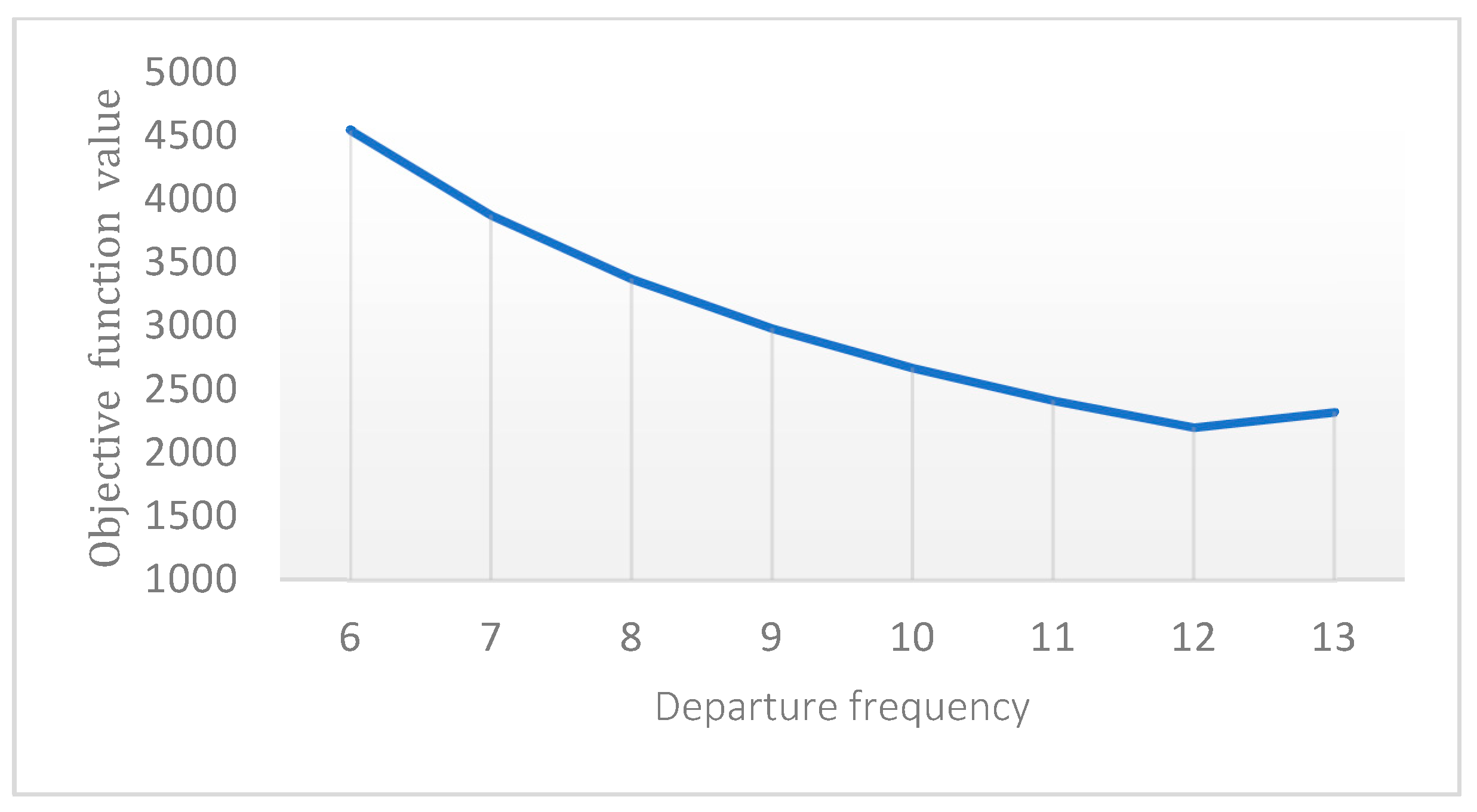
This paper investigated the basic data of bus route 207 of Nanchang city, China, and optimized the departure frequency and departure interval of the bus route in the morning peak hour based on uncertainty theory and a bi-level programming model. The uncertainty of passenger arrival and bus operation time was taken into account, combined with actual operation conditions. After determining the optimal departure frequency, the differences between uniform and non-uniform scheduling are studied and analyzed. Nanchang 207 bus line was taken as an example to optimize the departure frequency and scheduling in the morning peak hour. The optimal departure frequency in the morning peak hour is 12 times. The overall index value of the route non-uniform scheduling during peak hours increased by 0.06 and 9.23% compared with uniform scheduling. The analysis results show that the effect of the non-uniform scheduling is obvious.

Moreover, taking integers of model variables is conducive to the solution of the model and improves the practicability of the model. At the same time, the upper-level programming model can intuitively reflect the mutual influence and mutual restriction between the bus companies and passengers in the public transportation system. The problem of bus line departure frequency and scheduling has a positive effect on improving the efficiency of public transportation, reducing operating costs, and promoting the sustainable development of the public transportation system. This paper considers the uncertainty of the number of passengers at the bus station and the bus operation time and also considers the cost and benefits of bus operators as well as bus passengers. The uncertainty bi-level programming model for departure frequency of a bus line is more consistent with reality. Although the uncertain theory has been widely and successfully applied in the fields of transportation [16,17,18,19,20,21,22,23,24], the results of using the uncertainty theory to study the bus vehicle configuration problems are few. Therefore, this article provides a theoretical support for bus operators to optimize route operations.

However, the model assumptions are relatively ideal, and some influencing factors are not reflected in the model and need to be further discussed in future research. Nanchang Public Transport Group only provided the number of card swipes but unfortunately did not provide passenger attribute information. If relevant data can be obtained in the future, in-depth analysis of the impact of passenger attributes and economic and social background on public transportation travel can be conducted. The social (in) equity and housing along the bus line are not considered in the research. The captive riders of public transport are often middle-to-low-income residents, with high-income residents (the choice riders) often choosing to drive to reach various destinations. Housing price/cost is often a good indicator for the income level of residents living there and the probability of residents’ transit utility. Moreover, the optimization of transit location should consider the very people living along the transit lines, which can be relatively accurately reflected by housing costs/prices. In [29,30,31], housing and transit costs have been examined. Transit optimization is often a social equity issue that should be discussed in the future along with housing since they are often intertwined with each other in affecting (in) equity. The coupling factors of passenger travel demand and vehicle scheduling, the location, environment, platform capacity, passenger waiting time, and other attributes of the bus stop should also be fully considered. Zhichao Cao [32] considered the constraints of the vehicle with regard to capacity in shuttle bus service timetabling and vehicle scheduling. Man Li [33] considered the function of rail transit line capacity and load distribution strategy, the passenger flow congestion in a train delay scenario. When considering passengers choosing a bus, the model assumes that as long as the number of passengers in the bus does not reach the maximum capacity, then passengers could get on the bus, without considering the impact of the crowded situations in vehicles on passenger choice, which also affects the reliability of model calculation results. This study only analyzes departure frequency and scheduling and considers the uncertain variables of the number of passengers at the bus stop as well as running time; the optimization problem under multiple uncertain factors, such as the number of passengers at the bus stop, bus line assignments, and driving timetables, which constitute the optimization problem of driving operation plans, needs further research. The size of the test population and the flow frequency are not fully considered in the present manuscript; deeper work will be carried out in the future. In addition, the optimization of public transportation networks and regional dispatching considering uncertain factors are also worthy of discussion. Additionally, the situation especially in COVID-19 times, when the utilization of public transport is being re-defined to address the new safety standards, is not considered in the manuscript, which can be discussed in further research.

To summarize the research, this paper considers the uncertainty of the number of passengers at the bus stop and the bus operation time and also considers the cost and benefits of bus operators as well as bus passengers. An uncertain bi-level programming model was established with a view to providing theoretical support for bus departure time problems. The case study of bus route 207 of Nanchang city, China, shows the proposed uncertain bi-level programming model is effective for addressing the departure frequency problem of bus lines. As mentioned in the previous paragraph, this study has some limitations. Model assumptions and more influencing factors need to be further considered and improved.

References

1. Guo, L.J.; Ma, R.; Hu, Z. Urban Transit Network Properties Evaluation and Optimization Based on Complex Network Theory. Sustainability 2019, 11, 2007. [Google Scholar]
2. Damidavičius, J.; Burinskienė, M.; Antuchevičienė, J. Assessing Sustainable Mobility Measures Applying Multicriteria Decision Making Methods. Sustainability 2020, 12, 6067. [Google Scholar] [CrossRef]
3. Liu, T.; Ceder, A. Integrated public transport timetable synchronization and vehicle scheduling with demand assignment: A bi-objective bi-level model using deficit function approach. Transp. Res. Part B Methodol. 2018, 117, 935–955. [Google Scholar] [CrossRef]
4. Huang, Z.; Li, Q.; Li, F.; Xia, J. A Novel Bus-Dispatching Model Based on Passenger Flow and Arrival Time Prediction. IEEE Access 2019, 7, 106453–106465. [Google Scholar] [CrossRef]
5. Zhen, D. A Bi-Level Programming Model for Vehicle Allocation of Bus Lines; East China Jiaotong University: Nanchang, China, 2010. [Google Scholar]
6. Zhao, S.; Wang, D.; Liu, H.; Sun, J. Multi-vehicle-type Configuration Model of Regular Bus Lines. J. Beijing Univ. Technol. 2017, 43, 1529–1534. [Google Scholar]
7. Monnerat, F.; Dias, J.; Alves, M.J. Fleet management: A vehicle and driver assignment model. Eur. J. Oper. Res. 2019, 278, 64–75. [Google Scholar] [CrossRef]
8. Kang, L.; Chen, S.; Meng, Q. Bus and driver scheduling with mealtime windows for a single public bus route. Transp. Res. Part C Emerg. Technol. 2019, 101, 145–160. [Google Scholar] [CrossRef]
9. Goberna, M.; Jeyakumar, V.; Li, G.; Vicente-Pérez, J. Guaranteeing highly robust weakly efficient solutions for uncertain multi-objective convex programs. Eur. J. Oper. Res. 2018, 270, 40–50. [Google Scholar] [CrossRef]
10. Bakker, H.; Dunke, F.; Nickel, S. A structuring review on multi-stage optimization under uncertainty: Aligning concepts from theory and practice. Omega 2019, 96, 102080. [Google Scholar] [CrossRef]
11. Liu, B. Uncertainty Theory, 4th ed.; Springer: Berlin/Heidelberg, Germany, 2015. [Google Scholar]
12. Chen, W.; Wang, X.; Liu, M.; Zhu, Y.; Deng, S. Probablilistic Risk Assessment of RCC Dam Considering Grey-Stochastic-Fuzzy Uncercainty. KSCE J. Civ. Eng. 2018, 22, 4399–4413. [Google Scholar] [CrossRef]
13. Kolmogorov, A.N. Grundbegriffe der Wahrscheinlichkeitsrechnung; Julius Springer: Berlin, Germany, 1933. (In German) [Google Scholar]
14. Savage, L.J. The Foundations of Statistical Inference; Methuen: London, UK, 1962. [Google Scholar]
15. Liu, B. Uncertainty Theory, 2nd ed.; Springer: Berlin/Heidelberg, Germany, 2007. [Google Scholar]
16. Liu, B. Theory and Practice of Uncertain Programming, 2nd ed.; Springer: Berlin/Heidelberg, Germany, 2009. [Google Scholar]
17. Li, B.; Sun, Y.; Aw, G.; Teo, K.L. Uncertain portfolio optimization problem under a minimax risk measure. Appl. Math. Model. 2019, 76, 274–281. [Google Scholar] [CrossRef]
18. Jiao, D. Uncertain Programming Model for Vehicle Routing Problem; Tsing Hua University: Beijing, China, 2015. [Google Scholar]
19. Liu, W.; Liu, X.; Tan, Q. Uncertainty Analysis to Passenger Flow of Bus Stations Based on Multivariate Date Fusion. J. Transp. Syst. Eng. Inf. Technol. 2018, 18, 149–156. [Google Scholar]
20. Wei, M.; Sun, B.; Jin, W. A Bi-level Programming Model for Uncertain Regional Bus Scheduling Problems. J. Transp. Syst. Eng. Inf. Technol. 2013, 13, 106–112. [Google Scholar] [CrossRef]
21. Chen, L.; Peng, J.; Zhang, B. Uncertain goal programming models for bicriteria solid transportation problem. Appl. Soft Comput. 2017, 51, 49–59. [Google Scholar] [CrossRef]
22. Guo, J.; Xue, Y.; Guan, H. Research on the combinatorial optimization of EBs departure interval and vehicle configuration based on uncertain bi-level programming. Transp. Lett. 2022, 1–11. [Google Scholar] [CrossRef]
23. Zhang, B.; Zhong, Z.; Sang, Z.; Zhang, M.; Xue, Y. Two-Level Planning of Customized Bus Routes Based on Uncertainty Theory. Sustainability 2021, 13, 11418. [Google Scholar] [CrossRef]
24. Zhan, B.; Lu, H.; Yang, Y.; Li, R. Optimization of Departure Intervals Considering Uncertainty of Bus Passenger Flow Demand. J. Wuhan Univ. Technol. 2017, 41, 978–983. [Google Scholar]
25. Sun, L.; Lin, L.; Li, H.; Gen, M. Hybrid Cooperative Co-Evolution Algorithm for Uncertain Vehicle Scheduling. IEEE Access 2018, 6, 71732–71742. [Google Scholar] [CrossRef]
26. Ciccullo, F.; Pero, M.; Gosling, J.; Caridi, M.; Purvis, L. When Sustainability Becomes an Order Winner: Linking Supply Uncertainty and Sustainable Supply Chain Strategies. Sustainability 2020, 12, 6009. [Google Scholar] [CrossRef]
27. El-Geneidy, A.; Levinson, D.; Diab, E.; Boisjoly, G.; Verbich, D.; Loong, C. The cost of equity: Assessing transit accessibility and social disparity using total travel cost. Transp. Res. Part A Policy Pr. 2016, 91, 302–316. [Google Scholar] [CrossRef]
28. Liu, D.; Kwan, M. Measuring Job Accessibility Through Integrating Travel Time, Transit Fare And Income: A Study Of The Chicago Metropolitan Area. Tijdschr. Econ. Soc. Geogr. 2020, 111, 671–685. [Google Scholar] [CrossRef]
29. Kramer, A. The unaffordable city: Housing and transit in North American cities. Cities 2018, 83, 1–10. [Google Scholar] [CrossRef]
30. Liu, D.; Kwan, M.; Kan, Z.; Song, Y. An integrated analysis of housing and transit affordability in the Chicago metropolitan area. Geogr. J. 2021, 187, 110–126. [Google Scholar] [CrossRef]
31. Renne, J.L.; Tolford, T.; Hamidi, S.; Ewing, R. The Cost and Affordability Paradox of Transit-Oriented Development: A Comparison of Housing and Transportation Costs Across Transit-Oriented Development, Hybrid and Transit-Adjacent Development Station Typologies. Hous. Policy Debate 2016, 26, 819–834. [Google Scholar] [CrossRef]
32. Cao, Z.; Ceder, A. Autonomous shuttle bus service timetabling and vehicle scheduling using skip-stop tactic. Transp. Res. Part C: Emerg. Technol. 2019, 102, 370–395. [Google Scholar] [CrossRef]
33. Li, M.; Zhou, X.; Wang, Y.; Jia, L.; An, M. Modelling cascade dynamics of passenger flow congestion in urban rail transit network induced by train delay. Alex. Eng. J. 2022, 61, 8797–8807. [Google Scholar] [CrossRef]
Figure 1. The process of solution algorithm.
Sustainability 15 07005 g001
Figure 2. The stops and route distribution of bus line 207 in Nanchang city, China.
Sustainability 15 07005 g002
Figure 3. Relationship between departure frequency and objective function value in lower-level function.
Sustainability 15 07005 g003