Performance of Statistical and Intelligent Methods in Estimating Rock Compressive Strength

Abstract

This research was conducted to forecast the uniaxial compressive strength (UCS) of rocks via the random forest, artificial neural network, Gaussian process regression, support vector machine, K-nearest neighbor, adaptive neuro-fuzzy inference system, simple regression, and multiple linear regression approaches. For this purpose, geo-mechanical and petrographic characteristics of sedimentary rocks in southern Iran were measured. The effect of petrography on geo-mechanical characteristics was assessed. The carbonate and sandstone samples were classified as mudstone to grainstone and calc-litharenite, respectively. Due to the shallow depth of the studied mines and the low amount of quartz minerals in the samples, the rock bursting phenomenon does not occur in these mines. To develop UCS predictor models, porosity, point load index, water absorption, P-wave velocity, and density were considered as inputs. Using variance accounted for, mean absolute percentage error, root-mean-square-error, determination coefficient (R²), and performance index (PI), the efficiency of the methods was evaluated. Analysis of model criteria using multiple linear regression allowed for the development of a user-friendly equation, which proved to have adequate accuracy. All intelligent methods (with R² > 90%) had excellent accuracy for estimating UCS. The percentage difference of the average of all six intelligent methods with the measured value was equal to +0.28%. By comparing the methods, the accuracy of the support vector machine with radial basis function in predicting UCS was (R² = 0.99 and PI = 1.92) and outperformed all the other methods investigated.

1. Introduction

Stability of slopes, prediction of drilling rate, classification of rock masses, and modeling of foundations require knowledge of the uniaxial compressive strength (UCS) of the rocks for designing projects [1,2,3]. Indirect determination of the UCS in places where the preparation of standard samples is difficult requires lots of time and is expensive. Hence, various researchers have predicted the UCS of the limestones and sandstones using statistical and intelligent methods [4,5,6,7]. Aladejare et al. [8] collected empirical relationships and models between UCS and other rock characteristics from previous studies. Several models were developed to estimate the rock UCS using Gaussian process regression (GPR) [9,10,11,12,13], feedforward multilayer perceptron artificial neural network (FMP-ANN) [14,15,16,17,18,19], random forest algorithm (RFA) [20,21,22,23], adaptive neuro-fuzzy inference system (ANFIS) [24,25,26,27,28], and multiple linear regression (MPLR) [3,4,7,8,25,29,30,31]. The results of Lawal et al.’s [9] study showed that the GPR method, with a correlation coefficient of almost 100%, is able to estimate the static and dynamic properties of sedimentary rocks. Moreover, a comparison of the RFA, MPLR, FMP-ANN methods in compressive strength estimation showed that FMP-ANN with the Levenberg–Marquardt algorithm has a higher accuracy than other methods [20]. The results of Matin et al.’s [22] study to select the effective variables using the random forest method showed that compression wave velocity is the most effective variable as an input for estimating compressive strength and the modulus of elasticity using predictive models. Hudaverdi [25] stated that the ANFIS method has a high efficiency in flyrock estimation with an average error of less than 8%. The results of the MPLR, ANFIS, and FMP-ANN methods in the UCS estimation showed that all three methods have a determination coefficient higher than 90%, while the ANFIS method has a better performance [26]. The comparison of the ANFIS, FMP-ANN and multiple regression methods by Yesiloglu-Gultekin and Gokceoglu [26] showed that the ANFIS method has higher accuracy for estimating compressive strength and the modulus of elasticity.

Mahmoodzadeh et al. [32] compared the K-nearest neighbor algorithm (KNNA), Gaussian process regression based on squared exponential kernel (GPR-SEK), support vector machine with radial basis function (SVR-RBF), and decision tree (DT) methods to forecast rock quality designation in a tunnel project and stated that the GPR-SEK method is more accurate than other methods. Xu et al. [33] forecasted the UCS of rock using intelligent technics. The SVM-RBF was used to predict UCS [34]. Rastegarnia et al. [19] used FMP-ANN and MPLR to predict the UCS of carbonates. They stated that FMP-ANN estimates the UCS more than the measured value. Trott et al. [35] used RFA to classify rock types. Barzegar et al. [36] predicted the UCS of travertine rocks using the SVM-RBF, FMP-ANN, and ANFIS methods and stated that the SVM-RBF showed higher accuracy than the other methods. Mohamad et al. [37] estimated the UCS of soft rocks using FMP-ANN and particle swarm optimization (PSO)-based ANN. Madhubabu et al. [6] used MPLR and FMP-ANN to estimate the UCS of the carbonate samples. Umrao et al. [24] used the ANFIS approach for estimating UCS based on density, porosity, and PWV. Moreover, using inteligent methods, Gül et al. [17] predicted the UCS of different rock types. Singh et al. [38] estimated the UCS of basalt samples via MPLR and ANFIS. Kaloop et al. [39] used GPR and multivariate adaptive regression splines (MARSs) to estimate rock UCS. They stated that the MARS showed higher acuracy than the GPR method. Some engineers and researchers are interested in simple empirical relationships using simple models such as simple and MPLR to estimate UCS. Therefore, simple empirical relationships are widely used to estimate rock UCS using statistical methods.

Table 1. Relationships for estimating UCS by previous researchers.

Equation	Reference	Lithology
UCS = 12.29PLI1.233	Teymen and Mengüç [40]	Various Rocks
UCS = −37.82 + (0.017PWV)	Salehin [41]	Sedimentary Rocks
UCS = 0.043PWV − 136.8	Aldeeky and Al Hattamleh [42]	Basalt Rocks
UCS = 17.6PLI + 13.5	Aliyu et al. [30]	Sedimentary Rocks
UCS = 14.3PLI	Aladejare [8]	Sedimentary Rocks
UCS = 9.95PWV(1.21)	Kahraman [43]	Sedimentary rocks
$\mathrm{UCS}=0.034\mathrm{PWV}-86.36$	Wen et al. [7]	Limestone
UCS = −5.10$\varphi$ + 110.79	Edet [3]	Sandstone
UCS = 0.025PWV − 8.619	Azimian [29]	Limestone
UCS = 6.6PWV1.6	Uyanık et al. [44]	Sedimentary rocks
UCS = 22.18PWV − 30.32	Selcuk and Nar [31]	Various Rocks
UCS = 0.041PWV − 15.40	Abdi and Khanlari [4]	Sandstones
UCS = 2.304(PWV)2.43	Kılıç and Teyman [45]	Various Rocks
UCS = 10 − 5D16.7	Aladejare [8]	Sedimentary rocks

shows some of the relationships for estimating UCS by previous researchers.

This study was conducted to predict the UCS of sedimentary rocks based on porosity, point load index (PLI), density (D), water absorption by weight (WW), and P-wave velocity (PWV) using the FMP-ANN, GPR-SEK, KNNA, RFA, ANFIS, SVM, SR, and MPLR methods. Moreover, the types of kernel functions were investigated using the SVM method and the most accurate type of kernel function was introduced to estimate the UCS.

Sampling points, from 12 mines in the Bushehr province, south of Iran, are located between 50 and 52 degrees longitudes and 28 and 30 degrees latitudes. The mines are mainly travertine, limestone, and sandstone of the Aghajari and the Mishan formations.

2. Methodology

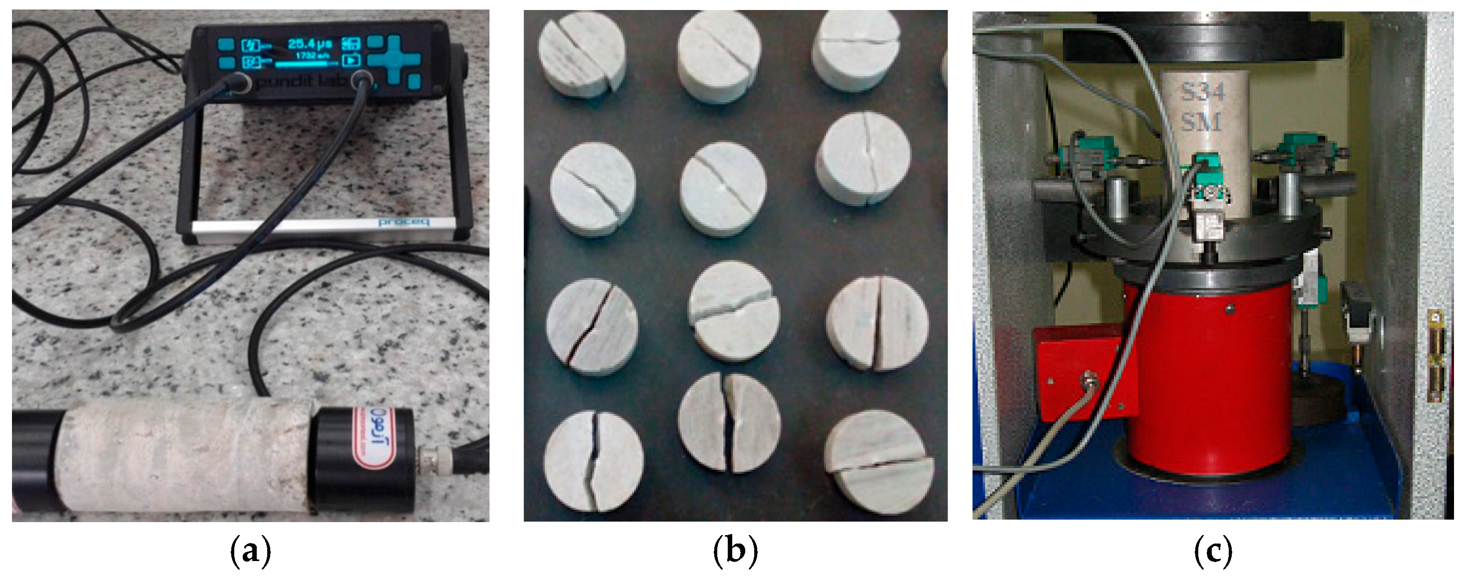
2.1. Laboratory Tests

Specimens with a diameter of 54 mm and a height to diameter ratio of 2 were prepared [46]. A wear device was used to parallel surfaces of specimens.

Table 2. Methods used for performing tests.

Test	Standards and References	Descriptions
UCS	ISRM [47]	A constant loading rate of 0.7 MPa per second was applied to the samples. The amount of deformation was recorded using the corresponding gauge in the UCS test.
Point load index (PLI)	ASTM D5731 [48]	This test was done on irregular and cylindrical samples. Then the PLI was calculated.
Compressional wave velocity test	ASTM D2845 [49]	With a ½ MHz frequency
Porosity ($\varphi$), density(D) and water absorption by weight (WW)	ISRM [47]	The total porosity ($\varphi$) of specimens was measured using the method of saturation and immersion way. Density was computed from the ratio of mass to sample volume.
Petrography	Folk [50], Dunham [51]	For classifying the samples using thin section images.

shows the methods used to measure geo-mechanical properties. Figure 1 displays some of the samples in laboratory tests.

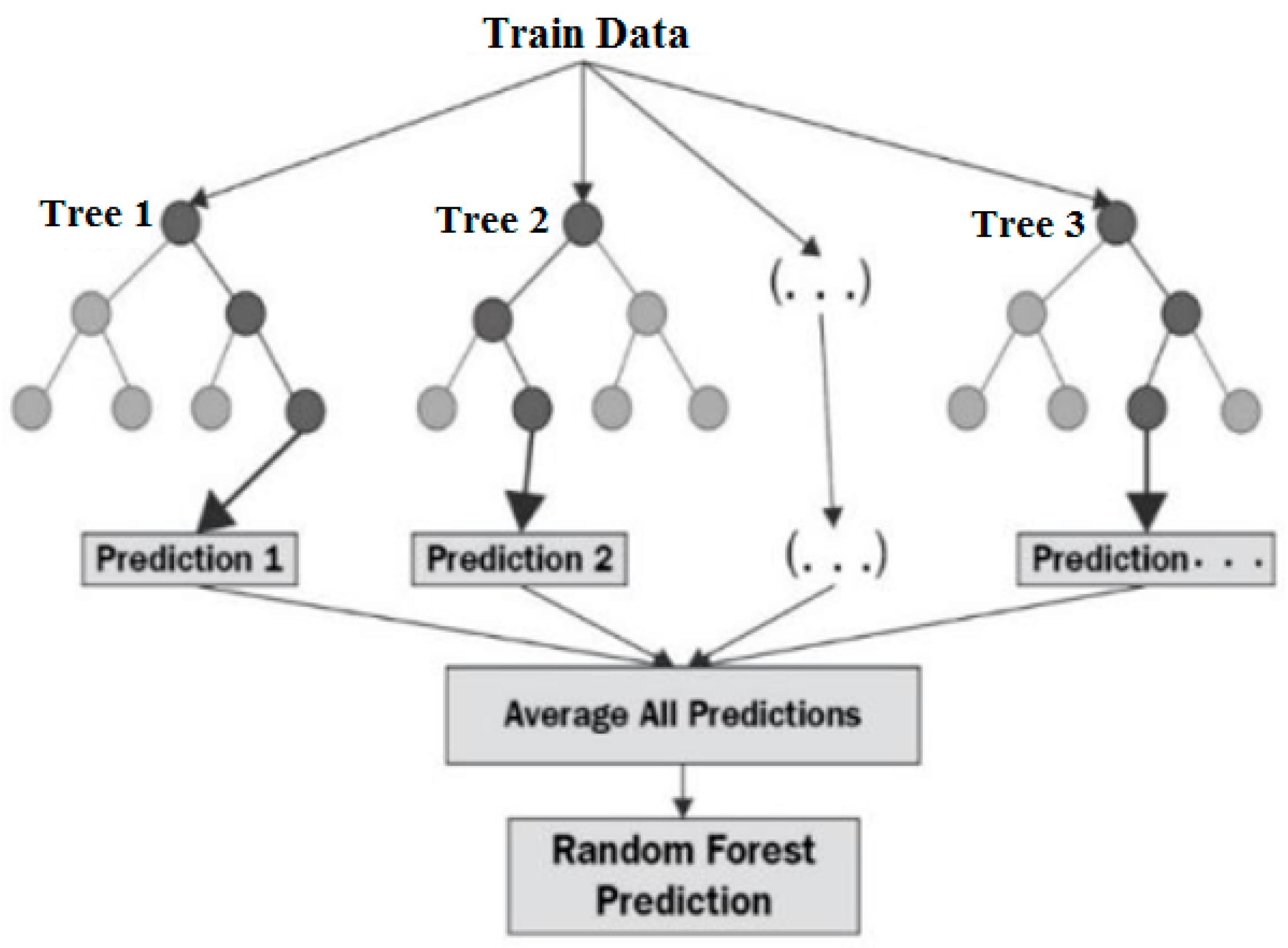
2.2. Random Forest Algorithm (RFA)

The random forest method is one of the ensemble methods. In these methods, the model chosen for classification or regression is a combination of several models. Figure 2 shows the idea of the random forest algorithm. In this approach, each model issues its vote and the final result about the value is issued based on these votes [22,23,52]. The general principles of group training techniques are based on the assumption that their accuracy is higher than other training algorithms [53]. On the other hand, the accuracy of combined methods is higher than the accuracy of its components [53]. The RFA method has also been used in rock mechanics in recent years [20]. In the RFA method, the models used in the combined method, which are all of the decision tree type, form a forest. Each of the decision trees is made using a random selection of special attributes in each node to determine the branching. In other words, each tree is built based on the values of a random vector. These values have the identical scattering for all trees in the forest and are sampled independently. For classification, each tree issues its vote, and the final result is determined by the majority vote [54]. The number of trees and the number of chosen variables in each node are important parameters in the RFA [55]. In this method, by replacing the information every sampling time, some information is never sampled, and other data may be sampled several times. In other words, some input data for some trees will be out of the bag, that is, they will not participate in the creation of some trees. These data have the function of an internal validator for each tree, which is performed by estimating the out-of-bag error. If the out-of-bag data itself is predicted through trees, there will be an error for these predictions, and the average of these errors is called the out-of-bag error. This error indicates the influence of the unselected samples on the error rate of the final result of the random forest [56].

2.3. Gaussian Process Regression Based on Squared Exponential Kernel (GPR-SEK)

Consider a d data set with n measurements: $d=\{(x_i,{ y}_i)|i=1,\dots ,n\}$, where x_i is the input vector with D dimension and y_i is the target output. This set, consisting of two components, input and output, will be denoted as measured points. To simplify the problem, the inputs of the collection are aggregated at $X=\{x_i,{ x}_2,\dots , x_n\}$ matrix and the outputs are also combined at $Y=\{y_i,{ y}_2,\dots , y_n\}$ matrix. Regression based on the data set d creates a new input x* to arrive at the predicted distribution for the corresponding values of the measured y* data. The Gaussian process (GP) is a group of accidental parameters, a restricted number of which are combined with Gaussian distributions (GDs) [57]. The GP is a generalization of GD. The GD is actually scattered between accidental parameters, while GP represents scattering between functions. The f(x) GP is described using the m(x) average and covariance functions according to Equations (1) and (2).

$$m\left(x\right)=E\left(f\left(x\right)\right)$$

(1)

$$c\left(x,x^{\prime }\right)=E\left(f\left(x\right)-m\left(x\right)\right)\left(f\left(x^{\prime }\right)-m\left(x^{\prime }\right)\right))$$

(2)

In relationships 1 and 2, $c\left(x,x^{\prime }\right)$ is the covariance or kernel function, which is computed at the x and $x^{\prime }$ points. The GP can be described as Equation (3).

$$f\left(x\right)\sim GP\left(m\right(x), \mathrm{c}(\mathrm{x},{\mathrm{x}}^{\prime }\left)\right)$$

(3)

Usually, for simplification, the value of the average function is considered equal to zero [58]. In the GP, the correlation between the target and the input vector is based on Equation (4).

$$y_i=f\left(x_i\right)+\epsilon$$

(4)

where $f\left(x_i\right)$ represents the arbitrary regression function and $\epsilon$ is the noise of the Gaussian function with zero mean and ${\sigma }^2$ variance (i.e., $\epsilon \sim N\left(0, {\sigma }^2\right)$). Furthermore, it is supposed that $f={\left[f\left(x_1\right), \mathrm{f}\left(x_2\right), \dots , \mathrm{f}\left(x_n\right)\right]}^T$ has a performance according to the GP (i.e., $p(f|X)=N\left(0, \mathrm{C}\right)$). Here, C is the covariance matrix with the $c_{i,j}=c\left(x_i,{ \mathrm{x}}_j\right)$ domains.

$$C\left(X,X\right)=\left(\begin{array}{c}c\left(x_1,x_1\right) c\left(x_1,x_2\right) \dots c\left(x_1,x_n\right)\\ c\left(x_2,x_1\right) c\left(x_2,x_2\right) \dots c\left(x_2,x_n\right)\\ \hspace{1em}⋮\hspace{1em}\hspace{1em}⋮\hspace{1em}\hspace{1em}⋮\hspace{1em}\hspace{1em}⋮\hspace{1em}\hspace{1em}\hspace{1em}\hspace{1em}\\ c\left(x_n,x_1\right) c\left(x_n,x_2\right)\dots c\left(x_n,x_n\right)\end{array}\right)$$

(5)

The $c_{i,j}$ is the covariance between the latent function values of $f\left(x_i\right)$ and $f\left(x_j\right)$. GP regression is used to calculate the predicted scattering for the f* function values in the test points of $X^{*}=\left[x_1^{*},x_2^{*} \dots x_m^{*}\right]$. The distribution of y depends on the values of f, which is represented by an isotropic Gaussian as follows.

$$p\left(y|f,x)=N(F,{\sigma }_n^{2}I\right)$$

(6)

In relation (6), I is the identity matrix. According to the characteristics of the Gaussian function, the marginal distribution of y is determined as follows.

$$p(y|X)={{\displaystyle \int }}^{ } p\left(y|f,X)p(f|X)df=N(0,C+{\sigma }_n^{2}I\right)$$

(7)

The integrated distribution of the observation data values, that is, the desired output, and the function values at the test points are written as follows [32].

$$\left[\begin{array}{c}y\\ f^{*}\end{array}\right]\sim N\left(0,\left[\begin{array}{l}C\left(X,X\right)+{\sigma }^{2}I C\left({X,X}_{*}\right)\\ C\left(X_{*},X\right) C\left(X_{*}{,X}_{*}\right)\end{array}\right]\right)$$

(8)

According to relation (3), and using standard rules to limit Gaussian, the following conditional distribution can be obtained.

$$p\left(f_{*}{|X,y,X}_{*}\right)\sim N\left(\overline{f_{*}},c(f_{*}\right))$$

(9)

$$\stackrel{-}{{\displaystyle f_{*}}}=C(X_{*},X){\left[C(C,C)+{\sigma }^{2}I\right]}^{-1}y$$

(10)

2.4. The SVM-RBF

To achieve the least error related to the test set, the SVM-RBF approach fits a linear line with epsilon ($\epsilon$) thickness on the data [59]. In this method, a function such as f(x) = m.x + b is used for forecasting, where m is weight vector and x and b are weights.

For minimizing weight vector and test error, this technique utilizes error functions for ignoring errors that are at a determined range from the real errors [60]. Hence, some deviation (derived from Equation (11)) from $\epsilon$ must be overlooked by including Equation (11) in Equation (12), which considers the ${\xi }_i^{-}$ and ${\xi }_i^{+}$ deficiency parameters. Finally, the error values are optimized via Equation (12) using structural error minimization

$${\left|\xi \right|}_{\epsilon }=\left[\begin{array}{c}0 if \left|\xi \right|\le \epsilon \\ \left|\xi \right|-\epsilon otherwise \end{array}\right]$$

(11)

$$\begin{gathered} \mathrm{Minimize}: \{(\Vert m{\Vert }^2)\ast 1/2\}+\{({\displaystyle \sum }_{i=1}^N({\xi }_i^{+}+{\xi }_i^{-}))\ast C\} \\ {\epsilon }_{\mathrm{Constrains}}: \left[\begin{array}{c}m.x_i+b+{\xi }_i^{+}-y_i\le \epsilon i=1, 2,.\dots , N\\ y_i-\left(b+m.x_i\right)\le {\xi }_i^{-}+\epsilon i=1, 2,.\dots , N\\ {\xi }_i^{+}\ge 0 , {\xi }_i^{-}\ge 0 i=1, 2,.\dots , N \end{array}\right] \end{gathered}$$

(12)

In Equation (12), $\{(\Vert m{\Vert }^2)\ast 1/2\}$ is the supervisory part, N is number of samples, $\epsilon$ is the allowable error, C is the complexity balance coefficient, and the ε values are the acceptable error range. As with the GPR method, various kernel functions are used in the SVM method [61]. Radial basis function (RBF), which is the most important kernel function, was used in the current research [62].

2.5. K Nearest Neighbor Algorithm (KNNA)

The KNNA is based on sample and performs classification based on K nearest neighbors. This method performs classification based on the similarity of the data. In fact, for each new test data, it calculates the K nearest neighbor distances and determines a label similar to the dominant label of this k neighbor for the desired point [63]. This method was introduced as a nonparametric method and does not make any assumption on the distribution of inputs. Therefore, it is extensively used in various fields [64].

In the KNNA classifier, an unknown value, is recognized by the similarity between known trained or labeled values based on the calculation of the distance between un-known values and labeled values. Then, K of the nearest values are selected as the basis for classification, and the unknown value (x test) is assigned to the class that has the most values among the closest values. For this purpose, three factors affect the KNNA classification: (1) the number of K of the neighbor and the changing of the value of K, which may amendment the classification results; (2) labeled dataset; therefore, adding or eliminating any value to the training samples affects the final results of the KNNA classifier; (3) the distance criterion. In KNNA, Euclidean distance is usually used as a distance criterion to measure the distance between two values [64,65]. This algorithm, as with the other algorithms used in this research, after examining the data in the program environment, divides the data into two parts, training data and test data, and builds the K nearest neighbor model and enters the training data into the model to train the model. Next, to determine the precision of the method, the test data is entered into the model for prediction and to evaluate the prediction accuracy in comparison with the labels of the test data [65,66].

2.6. ANFIS and FMP-ANN

The ANFIS and FMP-ANN methods have been widely introduced and described by previous researchers [18,25,67,68,69,70]. The transfer functions of neurons, membership functions, type of fuzzy inference system, and data training methods in these two methods are mentioned in the results section.

In the SVM-RBF, ANFIS, KNNA, GPR-SEK, and RFA methods, 30% and 70% of the whole data were used for the testing and training the models, respectively.

2.7. Performance Evaluation of Results

To appraise the methods, the correlation coefficient, the MAPE %, the RMSE, VAF, and the PI are defined in the form of Equations (13)–(16).

$$\mathrm{MAPE}=\frac{1}{n}{\displaystyle \sum }_{i=1}^n\left|\frac{y-y^{\prime }}{y}\right|\ast 100$$

(13)

$$RMSE=\frac{1}{s^{2}n}{{\displaystyle \sum }}_{i=1}^n{(y-y^{\prime })}^2$$

(14)

$$VAF=100\left[1-\frac{\mathit{var}(y-y^{\prime })}{\mathit{var}(y)}\right]$$

(15)

PI = R² + (VAF/100) − RMSE

(16)

In relationships 13 to 16, y is the value of the variable measured, $y^{\prime }$ is the predicted UCS, and n is the total data and $s^2$ is the sample variance. Equation (17) was used to normalize the data between −1 and 1.

$$X_i=2\left(\frac{X-X_{min}}{X_{max}-X_{min}}\right)-1$$

(17)

In Equation (17), x is the measured variable, X_min is the minimum of the data, and X_max is the maximum of the data.

3. Results and Discussion

3.1. Geomechanical Properties of Samples

The maximum, minimum, and average engineering properties of 65 samples (37 samples of limestone, 11 samples of argillaceous limestone, and 17 samples of sandstone) are presented in

Table 3. Laboratory results on sample.

	Properties	Density (g/cm3)	PLI (MPa)	Water Absorption (%)	Porosity (%)	UCS (MPa)	Es (GPa)	PWV (km/s)
Statistics
Average		2.43	3.75	6.81	9.44	37.54	14.95	4.38
Std. Dev.		0.11	1.66	1.87	3.35	16.49	5.30	1.03
Kurtosis		0.13	(0.58)	(0.50)	(0.41)	(0.58)	(0.51)	(0.38)
Skewness		(0.42)	0.09	0.70	0.79	(0.71)	(0.62)	(0.78)
Min.		2.10	0.31	4.08	4.36	4.12	3.00	2.06
Max.		2.63	8.00	11.00	16.72	59.72	22.90	5.79
Specimens		65	65	65	65	65	65	65

. The average Es and UCS are 14.95 GPa and 37.54 MPa, respectively. Physical, mineralogical, and petrographic characteristics cause changes in the compressive strength of rocks [5,18,71]. Moreover, lithological properties such as the type of rock, the amount and type of minerals, the type of cement between the particles that comprise the rock and physical properties such as the amount of moisture, porosity, and water absorption have a significant effect on the compressive strength and, consequently, on the stability of mines [72,73]. As the amount of clay minerals increases, the resistance of the samples decreases [4,74]. Water absorption causes the swelling and instability of the mine wall in samples with a high percentage of clay minerals [75,76,77]. The number of joints changes the geomechanical properties and instability of the rocky slopes [78,79,80]. The engineering properties and stability of structures are affected by the amount of moisture [81].

In the sandstone samples of the present research, clay and gypsum were found. The cement of the samples is gypsum and calcite. The grains of these sandstones are semi-rounded to angular and have a moderate to poor grading. The study of the thin sections of the samples showed that the samples with higher clay content show lower resistance characteristics. Swelling clay minerals (such as montmorillonite) were not observed in the investigated samples. Generally, rock bursting occurs in deep mines and in quartz-rich rocks [12]. Because the depth of the studied mines is less than 50 m and the overburden stress is negligible, the risks of rock bursting have not been reported in them so far.

3.2. Petrographic Features

Texture has a special effect on the engineering properties of sedimentary rocks [82]. In carbonates, the rock texture is very different, but their mineralogy is not much different [83,84]. According to microscopic studies, the most basic mineral of limestone rocks was calcite. Mishan formation limestone rocks, with an early Miocene age, based on the Dunham [51] classification, were classified in the range of mudstone to grainstone. Moreover, argillaceous limestone samples of this formation were classified in the mudstone to packstone categories. Sandstone samples of the Aghajari formation with an upper miocene age were classified as calc-litharenite according to the Folk [50] classification. These rocks consist of carbonaceous rock fragments (26 to 75), volcanic gravel (2 to 35%), meta-morphic fragments (2 to 18%), feldspar (1 to 10%), dark minerals (1 to 8%), quartz (0 to 22%), and chert (2 to 11%).

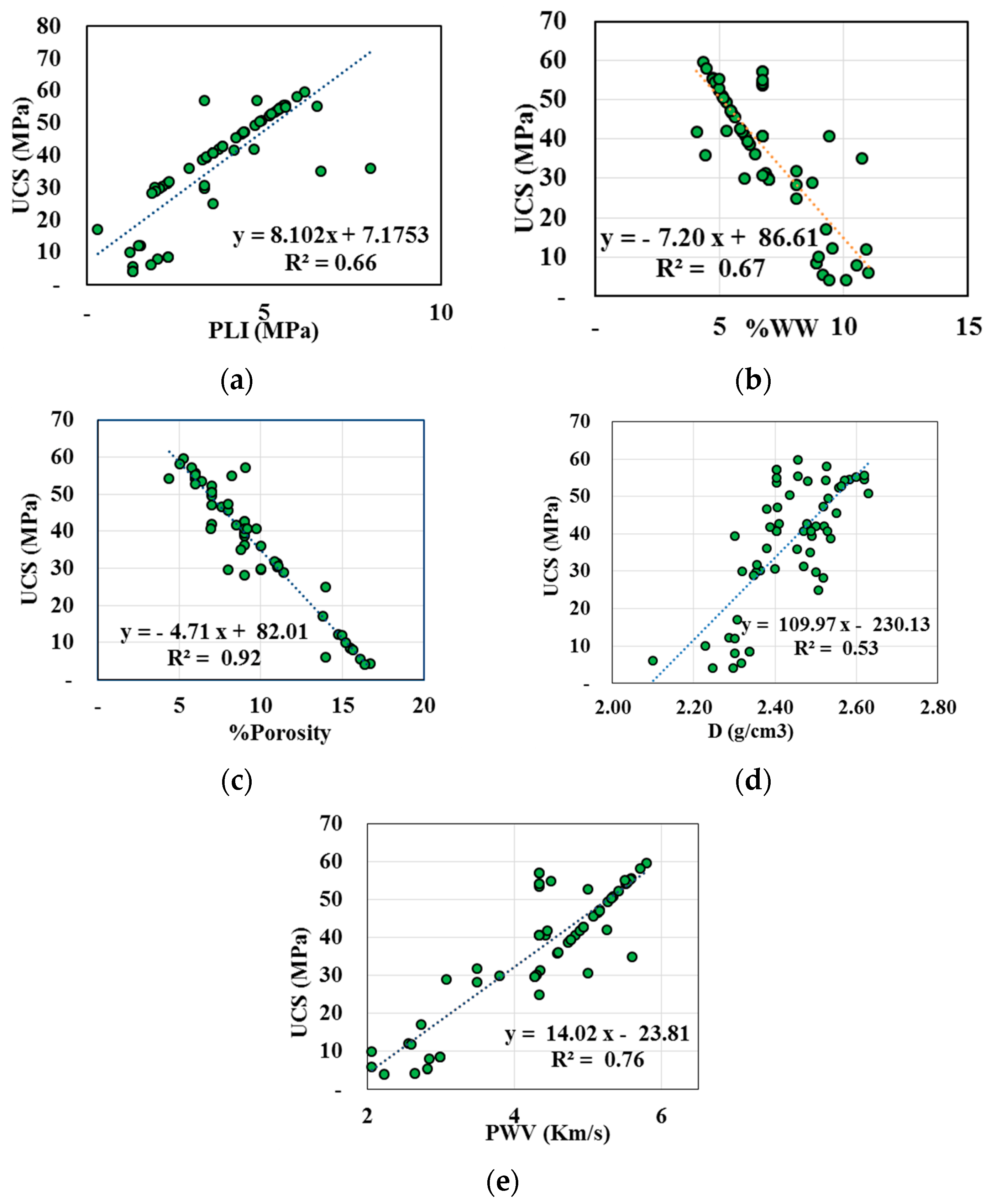
3.3. Influence of Independent Variables on the UCS

Figure 3 shows the effect of variables on the UCS. There is a reasonable tendency among these characteristics. The UCS decreases with increasing WW and porosity. This Figure shows that porosity has the highest effect on the UCS. Numerous studies have reported linear relationships with high accuracy between the point load index (PLI) and UCS [8,30]. The results of the relationship between PVW and UCS show that PWV displays a high accuracy to estimate UCS (Figure 3).

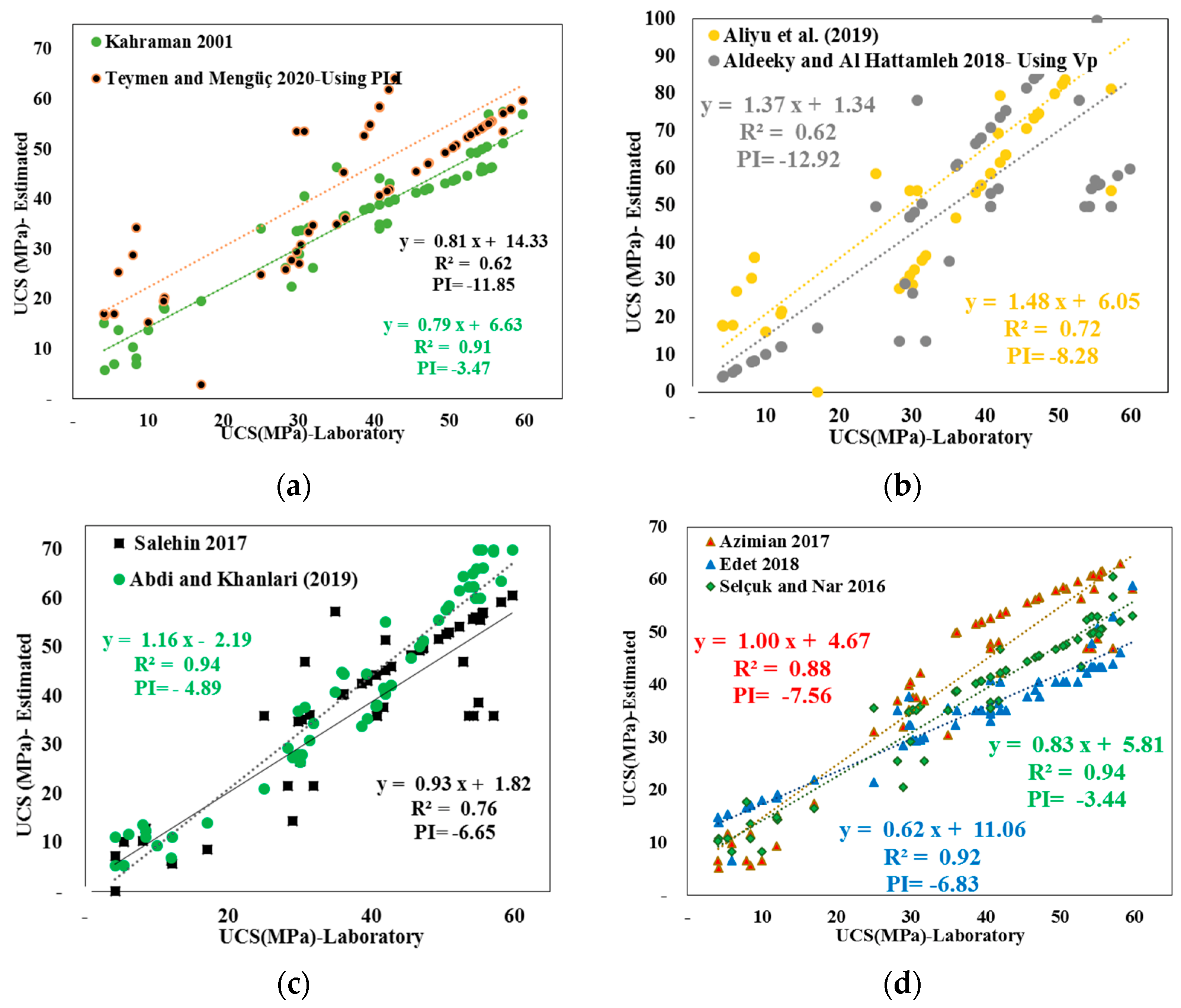
3.4. Evaluation of Previous Emperical Relationships

For predicting the UCS of the rocks, some empirical relationships have been proposed (Table 1). In the current research, for each of the 65 samples of the present study, based on each of the empirical relationships in Table 1, UCS was predicted. Finally, the accuracy of the forecasted and actual UCS relationships were assessed.

Figure 4 displays the data scattering and the precision of correlation using PI and R². The results revealed that there is good compatibility between actual UCS and the estimated one using previous studies (Figure 4). A performance index (PI) was introduced by Yagiz et al. [85] for evaluating empirical equations and models. The value of this index is equal to two in the best case, and the lower it is, the lower the relationship performance. As can be seen, although the correlation coefficient is high, the performance index is negative, which indicates the poor performance of the previous researchers’ relationships in estimating the UCS of the studied rocks (Figure 4). For this reason, various researchers have emphasized that empirical relationships should be determined for each region [85].

The type of rock, strength amount, method of conducting experiments, the test conditions (such as loading rate), and the petrography of the specimens of a specific study reveal the applicability of the proposed relationships for forecasting the UCS of rocks in other regions. For example, the average UCS of the samples of Edet [3] study was 32.22 MPa, and the average UCS of the present study is 37.54 MPa, which shows that the resistance of the Edet [3] study samples is lower than the resistance of the current research samples. As a result, the UCS values estimated from this researcher’s relationship are mostly below the diagonal line (Figure 4d). The sample breaks faster and shows more resistance when the loading rate is increased.

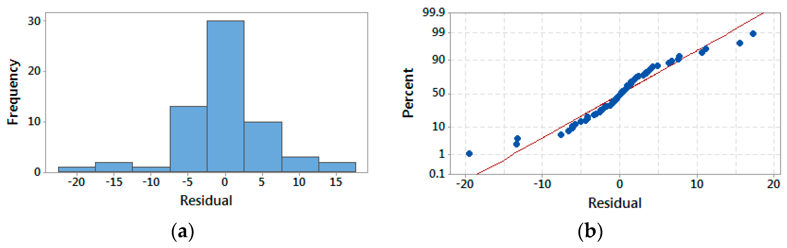
3.5. Multiple Linear Regression (MPLR)

In the current work, MPLR analysis was performed using Minitab software (version 18). Equation (18) was developed to predict the UCS using this method. Various criteria to evaluate this relationship are presented below.

Various statistics (

Table 4. Multiple linear regression results to estimate UCS and Es.

Equation	R2	RMSE (MPa)	MAPE%	VAF %	PI	DWS	ANOVA Results	Eq. No.
UCS = 5.03PWV − 1.735$\varphi$ + 2.667PLI	0.88	1.10	1.08	87.85	0.66	1.93	F-value = 79.37 p-value = 0.00	(18)

and

Table 5. Evaluation criteria of coefficients for relationship 18.

Term	Coefficients	T-Value	Significant Level (Sig.)	VIF (Variance Inflation Factor)
Constant	−32.1	−1.34	0.187	-
PWV	5.03	2.44	0.018	7.58
D	21.4	1.82	0.074	3.02
WW	0.281	0.35	0.728	3.81
$\varphi$	−1.735	−3.97	0.000	3.64
PLI	2.667	3.05	0.003	3.77

) were used to evaluate relationship 18. The Durbin–Watson statistic DWS) and variance inflation factor (VIF) are used to evaluate the independence of errors and the correlation of independent variables, respectively [86]. The results showed that there is no problem in using relationships in terms of these two criteria because the DW is in the range of 1.5 to 2 and the VIF value is less than 10 (Table 5). Analysis of variance (ANOVA) results (Sig. < 0.00) show that the model has been well developed using MPLR. Sig. values (related to T-test) in Table 5 indicate the presence of variables in the multivariate regression output relationship. The constant value, density, and water absorption were removed from Equation (18) because the sig. value is more than 0.05.

The normality of the error distribution is also one of the other criteria for evaluating empirical relationships. The normal distribution of errors related to the model provided by MPLR method shows that the proposed model can be used to estimate UCS (Figure 5).

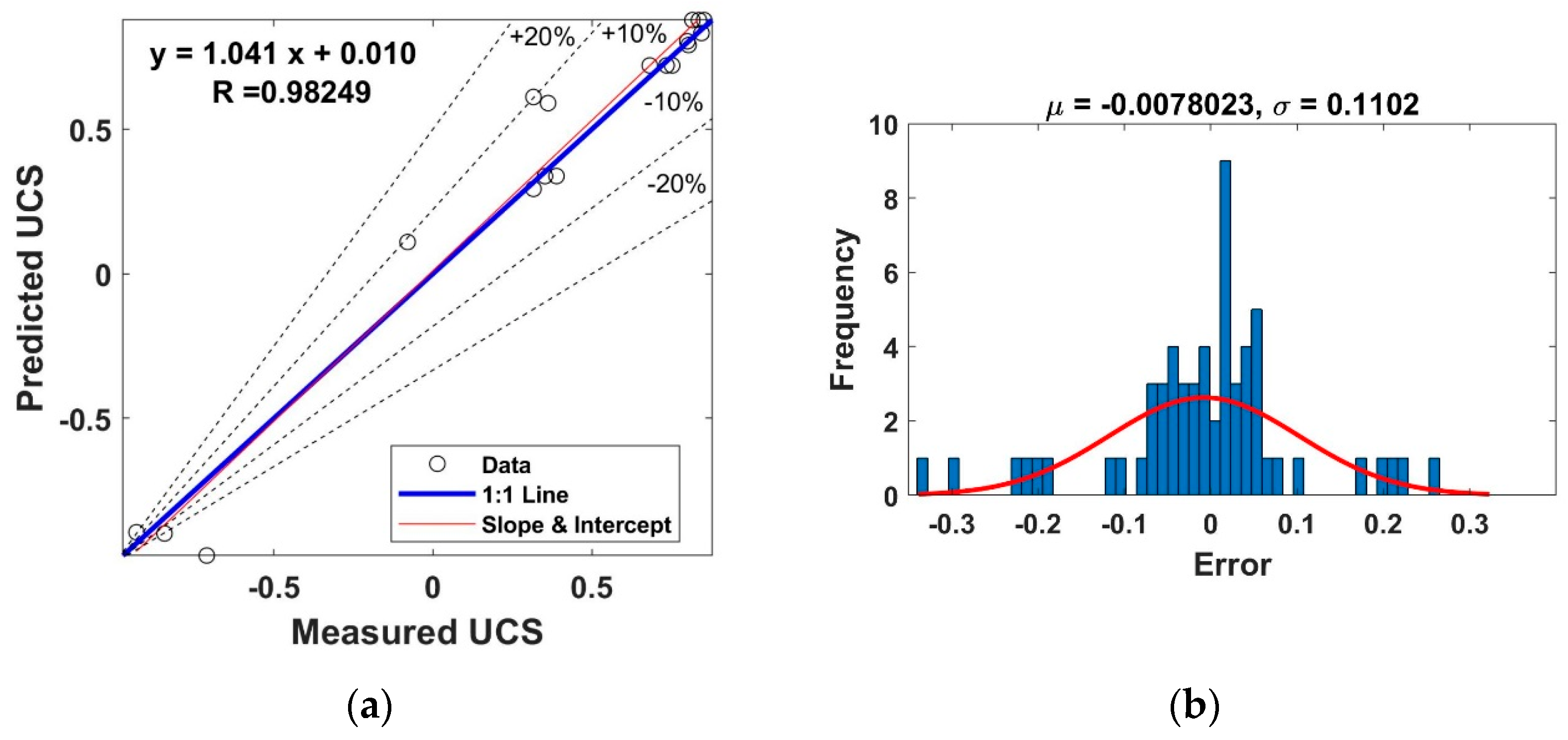
3.6. The Results of Modeling Using RFA and GPR-SEK Methods

The RFA modeling was conducted using the R (version R4.2.1) software [54]. The GPR-SEK model was conducted using MATLAB software (MATLAB 2016b). In the RF method, the 10-fold cross-validation method was used to control the number of chosen parameters in each node of tree (m-try) and the number of trees (n-tree). According to this method, the number of 500 trees and five variables in each node has delivered the most satisfactory conditions for modeling. Therefore, these values were used for modeling purposes.

The random forest method works well for large amounts of data and has high accuracy. In the random forest method, because the amount of error decreases with the increase of trees, 500 trees were used to develop the model. Upon model execution, the results were evaluated using an out-of-bag (OOB) error estimation. The model was appraised by the test data, the results of which are presented in Figure 6. One of the advantages of the random forest algorithm is that it can determine the importance of variables in a problem. In this research, the significance of the inputs was achieved using the Gini significance index [54]. The results showed that porosity has higher importance than other parameters. In Figure 6, the error histogram, the graph of the measured, the forecasted UCS using the RFA method, and the GPR-SEK model are drawn. The GPR-SEK model was implemented based on the squared exponential kernel function. As can be seen in the figure, the results are close to the bisector line, and it can be said that the values have been predicted with good accuracy. Theoretically, if R² equals 100%, all the observed values will be similar to the fitted values and all the data points will be on the fitted line [87].

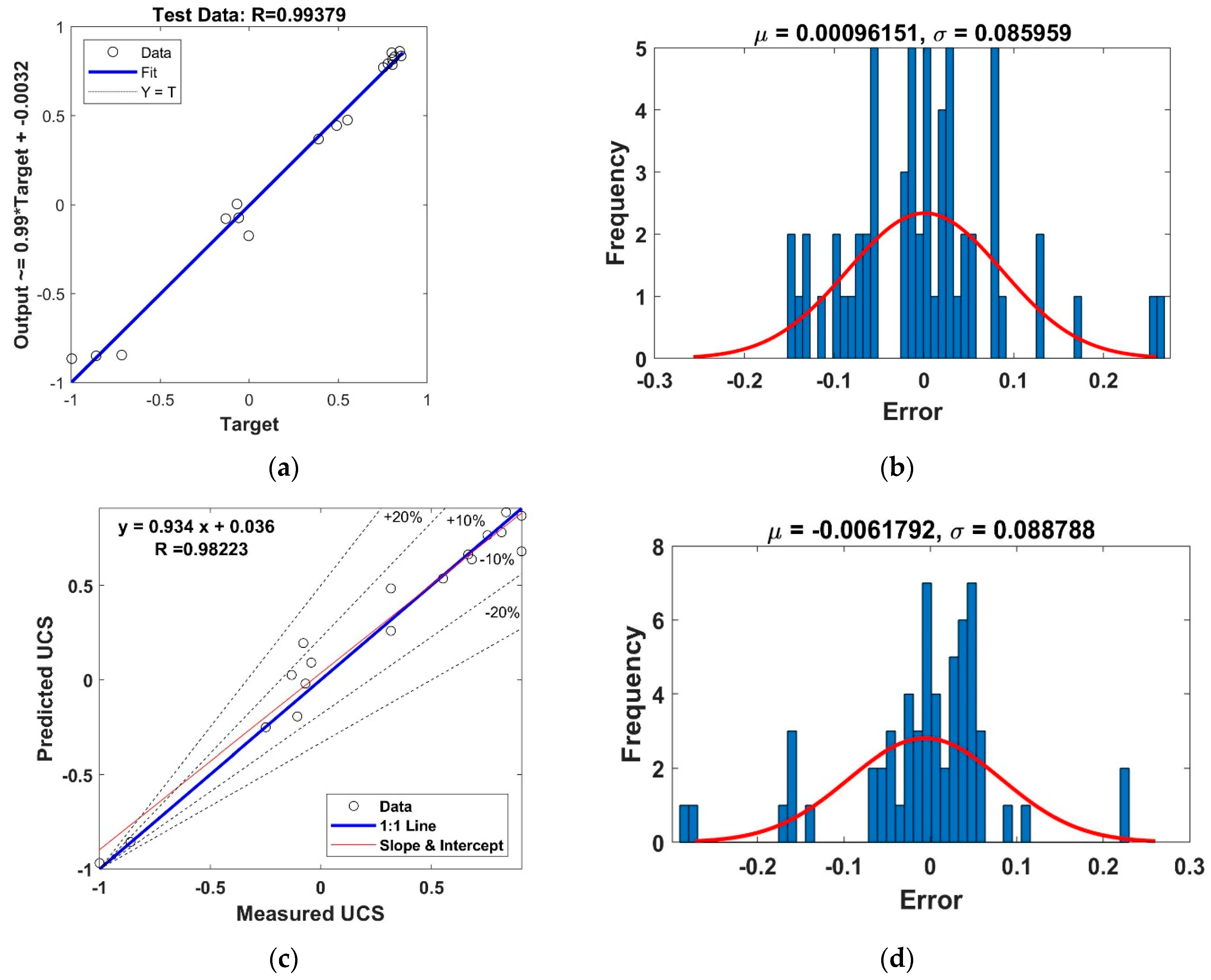
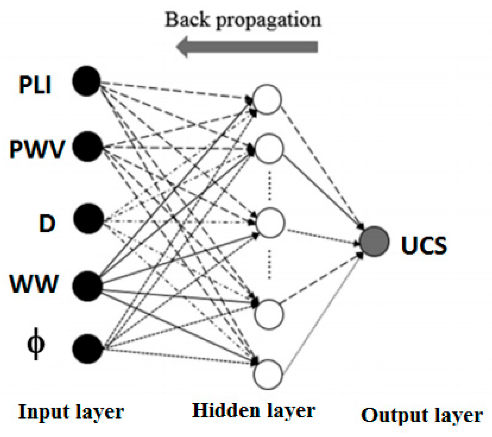
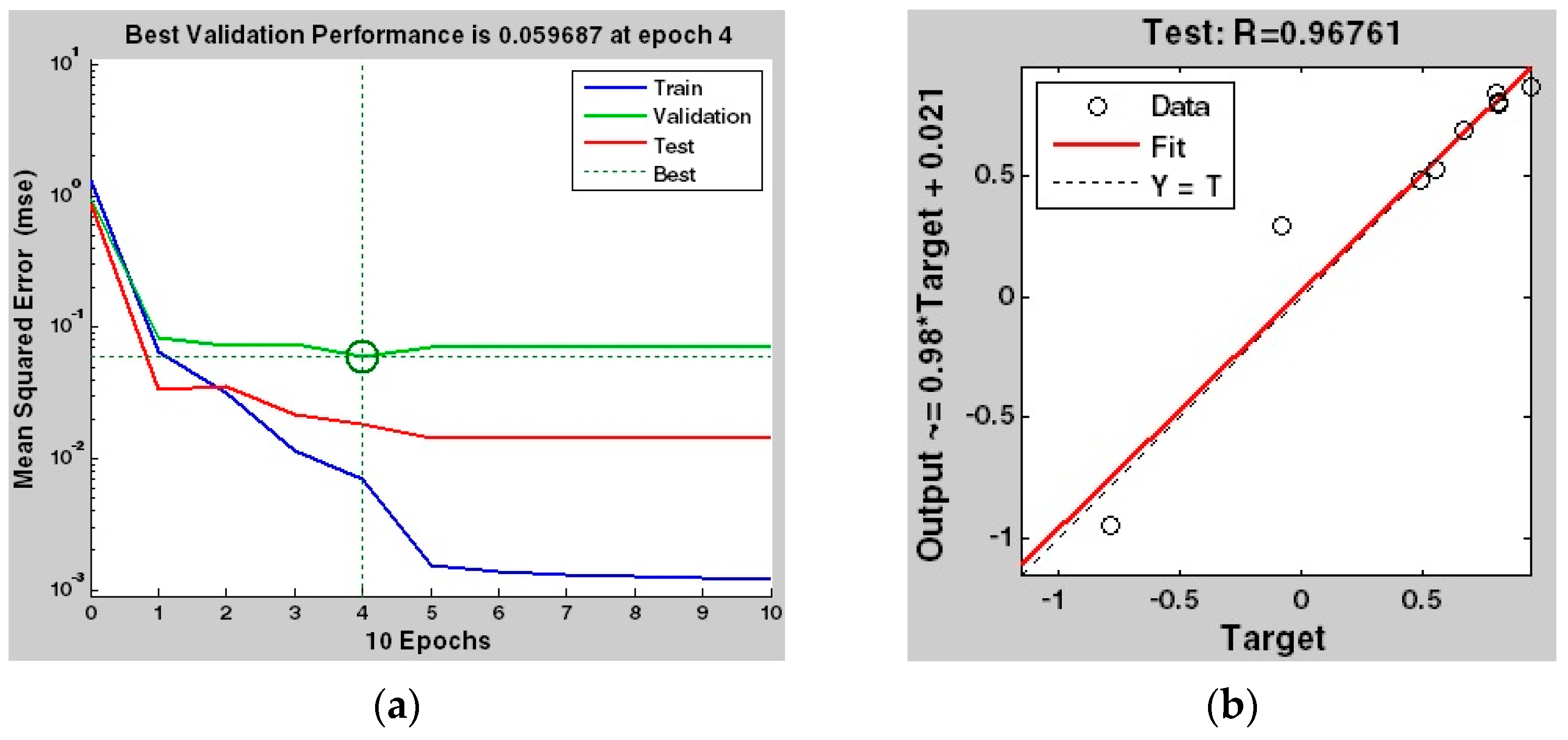
3.7. The FMP-ANN Results

The FMP-ANN is widely used in engineering [88,89]. In the current study, for predicting UCS, various neurons in a hidden layer were investigated to develop optimal models. Based on equations proposed by previous researchers, the number of hidden layer neurons changes were determined (

Table 6. Proposed equations by previous researchers to estimate the number of hidden layer neurons.

References	Neuron Numbers Calculated for This Study	Equations
Hecht-Nielsen [90]	$\le$3	≤$2\ast N_i+1$
Hush [91]	3	$3N_i$
Ripley [92]	3	$(N_i+N_0)/2$
Paola [93]	11	$\frac{2 + N_i \ast N_0 + 0.5N_0 \ast \left(N_0^2 + N_i\right) - 3}{(N_i + N_0)}$
Wang [94]	1	$2N_i$/3
Kaastra and Boyd [95]	2	$\sqrt{N_0\ast N_i}$
Kanellopoulos and Wilkinson [96]	1	$2N_i$

N₀ and N_i are the numbers of input and output neurons, respectively.

). The calculated number of hidden layer neurons changed from one to eleven according to Table 6. In this study, by checking this range using the FMP-ANN, this range was evaluated to achieve the ideal model architecture for forecasting UCS.

The used FMP-ANN method has a hidden layer with five inputs (PWV, point load index (PLI), porosity, density, and water absorption) and one output (UCS). Using MATLAB software, the Levenberg Marquardt (LM) training algorithm was used to train the network. The neuron transfer functions were the selected Sigmoid between the input layers and hidden layers and the Purelin between the hidden layers and output layers. In FMP-ANN modeling, the percentages of the validation, test, and training data in the present study were randomly selected as 15%, 15%, and 70% of the total data, respectively. The validation set is used to prevent overfitting, the training group is used to determine weights, and the test group is used to evaluate the FMP-ANN results [97,98,99,100]. The results showed that the third neuron is the most accurate neuron for estimating UCS. Figure 7 displays the optimal FMP-ANN chart achieved in the current research.

Figure 8 shows the error variations in optimum results. The lowest error in epoch 4 was obtained for predicting the UCS (Figure 8). Moreover, in this research, the results of the FMP-ANN to estimate UCS have been compared with several methods. It was found that the accuracy of all methods was very high (the coefficient of determination is more than 97%).

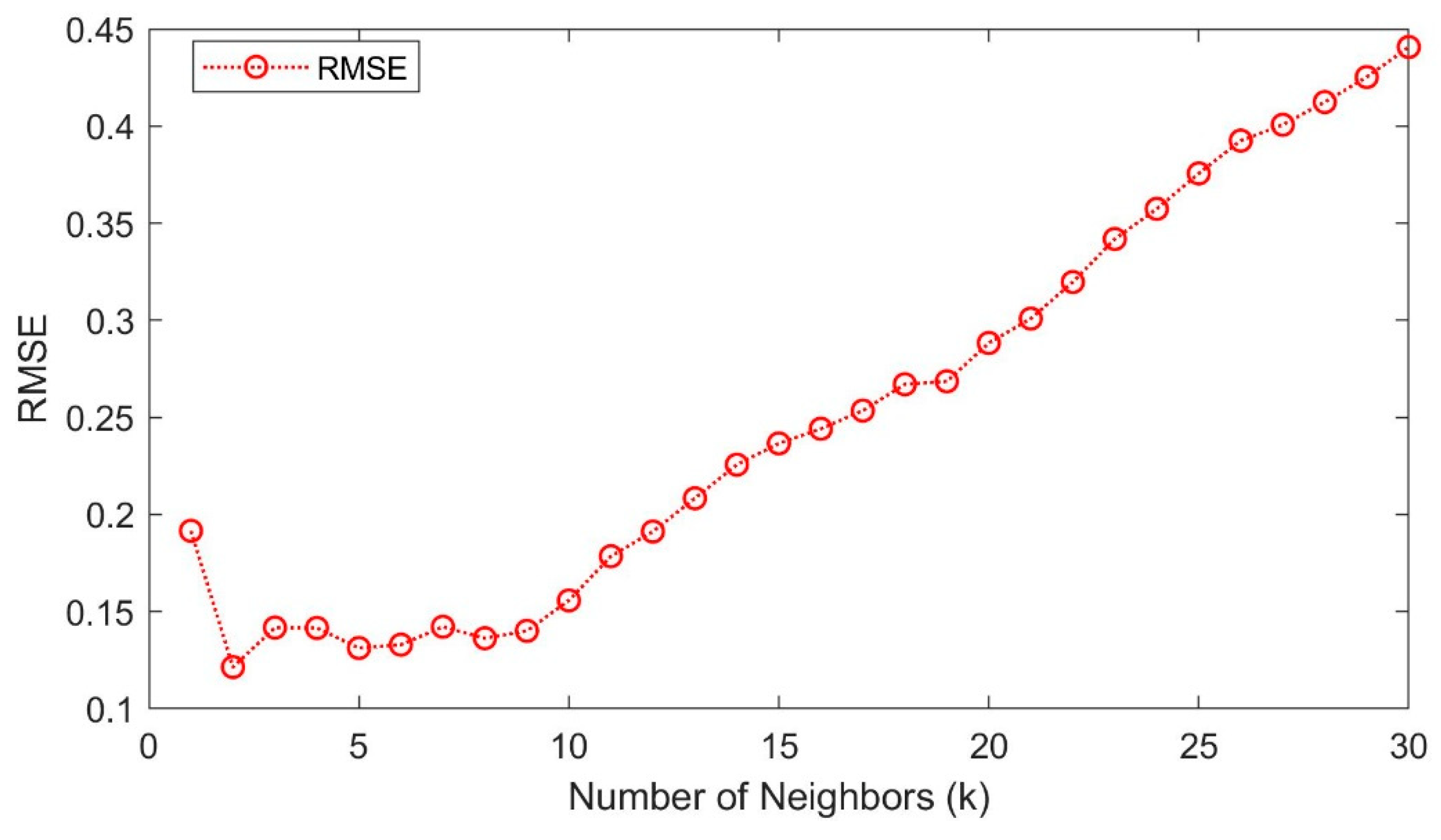
3.8. The KNNA Results

To apply the KNNA method to the data and determine the best K value, the KNNA was written in the form of a program in MATLAB software, which was run 310 times for K values from 1 to 30 programs; moreover, the amount of error was measured (Figure 9). Of the total data, 70% and 30% were used to train and test the model. The results showed that the lowest estimation error of the UCS was obtained at K = 2 (Figure 9). The error of this network for estimating the UCS with respect to the K values is equal to 0.11 (Figure 10). Figure 10 shows the KNNA results for estimating the UCS.

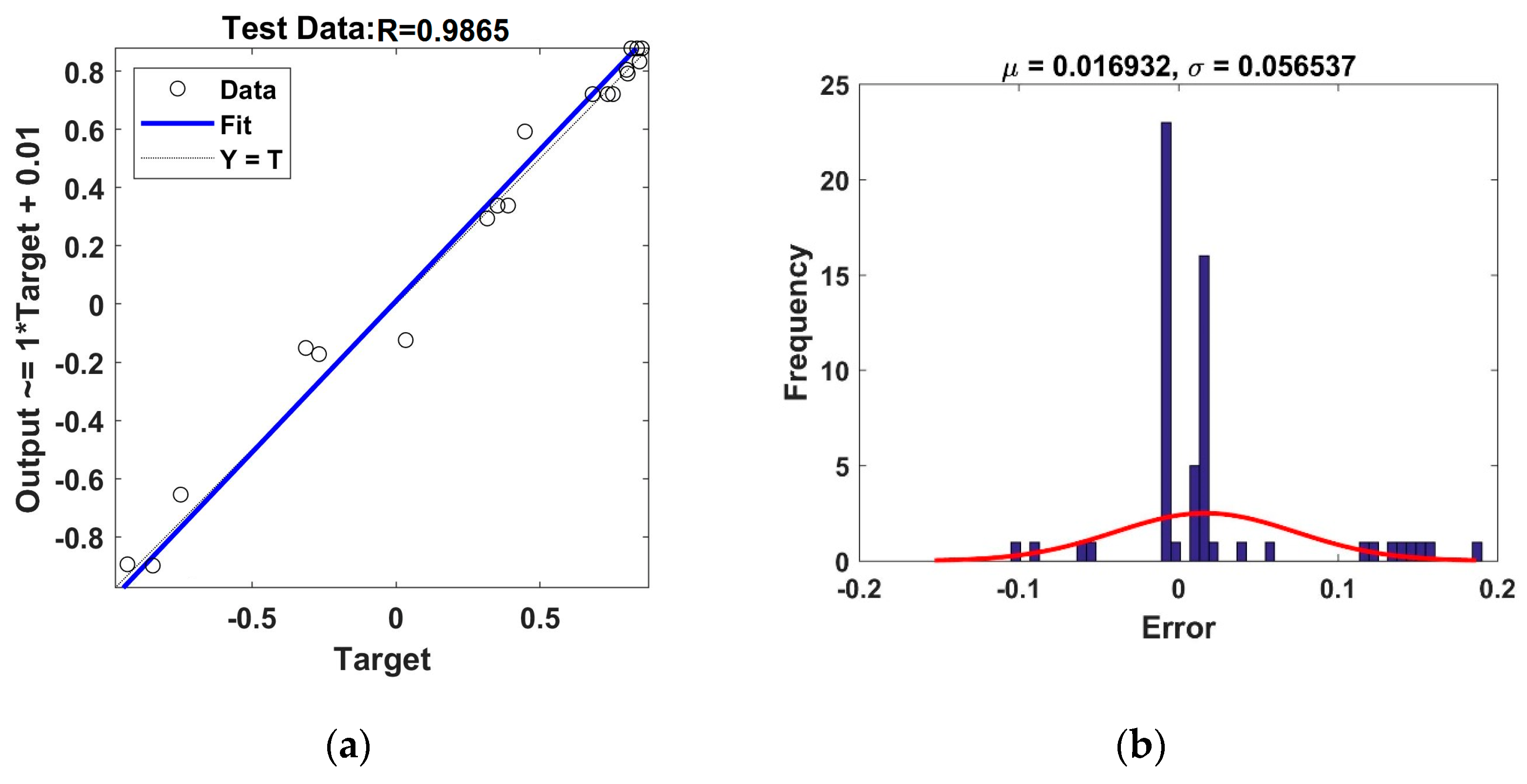
3.9. Results of SVM Method for Estimating UCS

The SVM algorithm uses a set of mathematical functions that are named kernels [101]. The most important kernel functions for solving engineering problems are listed in

Table 7. The most important kernel functions for solving engineering problems [102].

Function	Description	Kernel Function Type
$k\left(x_i,x_j\right)={(x_i.x_j+1)}^d$	This kernel is widely used in image processing, where d is the degree of the polynomial.	Polynomial kernel (PK)
$k\left(x_i,x_j\right)=\mathit{exp}(-\gamma \Vert x_i-x_j{\Vert }^2)$	This kernel is used for general purposes. It is used when there is no prior knowledge about the data. In $\gamma >0$ condition, $\gamma =1/2{\sigma }^2$ parameter is used.	Radial basis function (RBF)
$k\left(x_i,x_j\right)=x_i.x_j$	-	Linear kernel (LK)

. Normally, three radial basis kernel functions (RBFs), polynomial of degree, d, and linear, are used in the support vector machine, and the use of each of these functions with different parameters in the estimation of rock strength may lead to different results [60,101]. Therefore, it is necessary to evaluate the efficiency and accuracy of each of these functions and to choose the appropriate kernel function in predicting resistance. These three kernel functions were also used in this research. It should be mentioned that the calculation process of SVM was performed based on coding in a MATLAB environment and that the parameters of the kernel functions were optimized using a trial and error process. The results of these investigations are presented in

Table 8. Evaluation of SVM model performance in UCS estimation using various kernel functions.

Kernel Function	Optimal Values of Parameters					Test Period				Train Period
	$\mathit{\epsilon }$	t	d	$\mathit{\sigma }$	c	RMSE	R2	PI	MAPE	RMSE	R2	PI	MAPE
PK	1.72	280.01	4	-	12.12	0.08	0.97	1.87	2.86	0.07	0.98	1.84	2.81
RBF	0.02	-	-	1.10	27	0.06	0.99	1.90	2.82	0.06	0.99	1.90	2.80
LK	0.45	-	-	-	0.90	0.09	0.96	1.83	2.84	0.09	0.97	1.81

. It can be observed that, based on the statistical criteria, the accuracy of the kernel functions is as RBF> PK > LK. In this regard, Nguyen [102] investigated the performance of various kernel functions using the support vector machine method in estimating blast-induced ground vibration and stated that the radial basis function has the highest performance.

The error histogram and predicted and estimated UCS relationship with the optimal function (RBF function) are presented in Figure 11.

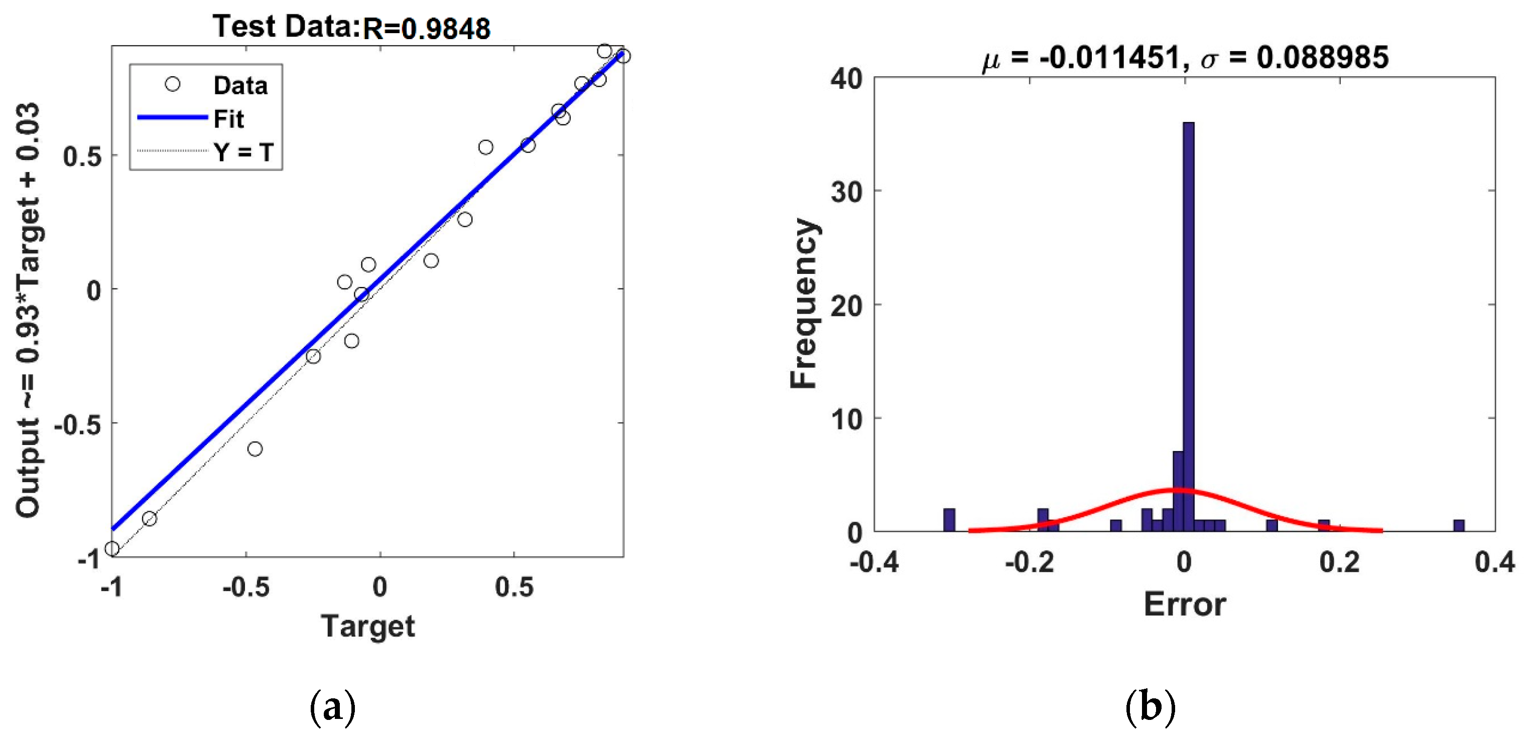
3.10. Results of ANFIS Method for Estimating UCS

As with other intelligent methods, to test and train models using ANFIS, 30% and 70% of the whole data were used, respectively. The method of combining regression error propagation with least squares was used to train the model using the ANFIS.

Table 9. Modeling features using ANFIS.

FIS Generation Method	GENFIS4
Influence radius	0.60
Number of epochs	500
Error goal	0.00
Type	Sugeno
Rules	4
Number of membership functions (MFs)	6
Input MF type	Gauss MF
Output MF type	Linear

shows the modeling features using the ANFIS method. A comparison of the performance of the methods for forecasting UCS based on different criteria has been reported in the next section.

Figure 12 shows the error histogram and correlation coefficient of the ANFIS model in the test stage. This method, as with other used intelligent methods, has high accuracy in UCS estimation. The results of the intelligent models for estimating UCS from the test data performed better than the training data; therefore, it can be argued that overfitting did not occur.

3.11. Evaluation of the Used Methods

Table 10. Accuracy of approaches for predicting UCS.

APPROACHES	MAPE%	R2	RMSE	VAF%	PI
RFA	9.27	0.98	0.09	97.63	1.87
SVM-RBF	2.83	0.99	0.06	98.96	1.92
ANFIS	2.98	0.98	0.09	97.86	1.87
KNNA	8.44	0.97	0.11	97.25	1.83
GPR-SEK	6.63	0.98	0.09	97.45	1.86
FMP-ANN	4.66	0.99	0.24	98.36	1.73

and Figure 13 show the accuracy of the used methods for forecasting the UCS. According to the statistical criteria (i.e., R², MAPE%, RMSE, VAF, and PI), the SVM-RBF model displays greater precision than other models because the SVM uses the minimizing structural risk theorem and adapts the ability of the model to existing training data [103]. The number of input variables, number of samples, and training algorithm type also affect the accuracy of the methods [16,104,105]. Based on the correlation coefficient, all methods (R² > 90%) have excellent accuracy for estimating UCS.

Considering that all six intelligent methods showed very high accuracy in UCS estimation, the percentage difference of the average of all six intelligent methods with the measured value in the laboratory is equal to +0.28%. This amount of difference is less than 1% and indicates the high capability of intelligent methods for forecasting the UCS.

4. Conclusions

The UCS of rocks is a basic parameter necessary for assessing the construction of civil and mining structures, such as the stability of the mines and the bearing capacity of foundations. UCS estimation using core specimens is costly, difficult, and, in some cases, impossible. After assessing the geo-mechanical features of 55 samples of sandstone, limestone, and argillaceous limestone specimens, predictive models for estimating UCS were developed via intelligent and statistical approaches. The results showed that the carbonate and sandstone samples were classified as mudstone to grainstone and calc-litharenite, respectively. The PWV, WW, porosity, density, and PLI were considered as model inputs for predicting UCS. Statistical analysis allowed the development of equations with high accuracy to estimate UCS. Among the assessed linear, polynomial, and radial basis kernel functions, the accuracy of the other models was lower than that of SVM-RBF in forecasting UCS. The SVM-RBF model revealed that the R² and PI values were 0.99 and 1.92, respectively. The R² values of 98%, 98%, 97%, 98%, and 99% for forecasting the UCS were achieved using ANFIS, RFA, KNNA, GPR, and FMP-ANN, respectively. The number of samples and input variables had a significant impact on the performance of the methods. When the number of samples was small, the SVM method was more accurate. The percentage difference of the average of all six intelligent methods with the measured value was less than 1%, which indicates the superior capability of the intelligent methods in forecasting UCS.

References

1. Yang, H.Q.; Zeng, Y.Y.; Lan, Y.F.; Zhou, X.P. Analysis of the excavation damaged zone around a tunnel accounting for geo-stress and unloading. Int. J. Rock Mech. Min. Sci. 2014, 69, 59–66. [Google Scholar] [CrossRef]
2. Yang, H.Q.; Xing, S.G.; Wang, Q.; Li, Z. Model test on the entrainment phenomenon and energy conversion mechanism of flow-like landslides. Eng. Geol. 2018, 239, 119–125. [Google Scholar] [CrossRef]
3. Edet, A. Correlation between Physico-mechanical Parameters and Geotechnical Evaluations of Some Sandstones along the Calabar/Odukpani–Ikom–Ogoja Highway Transect, Southeastern Nigeria. Geotech. Geol. Eng. 2018, 36, 135–149. [Google Scholar] [CrossRef]
4. Abdi, Y.; Khanlari, G.R. Estimation of mechanical properties of sandstones using P-wave velocity and Schmidt hardness. New Find. Appl. Geol. 2019, 13, 33–47. [Google Scholar]
5. Ajalloeian, R.; Mansouri, H.; Baradaran, E. Some carbonate rock texture effects on mechanical behavior, based on Koohrang tunnel data, Iran. Bull. Eng. Geol. Environ. 2017, 76, 295–307. [Google Scholar] [CrossRef]
6. Madhubabu, N.; Singh, P.K.; Kainthola, A.; Mahanta, B.; Tripathy, A.; Singh, T.N. Prediction of compressive strength and elastic modulus of carbonate rocks. Measurement 2016, 88, 202–213. [Google Scholar] [CrossRef]
7. Wen, L.; Luo, Z.Q.; Yang, S.J.; Guang, Y.Q.; Wang, W. Correlation of Geo-Mechanics Parameters with Uniaxial Compressive Strength and P-Wave Velocity on Dolomitic Limestone Using a Statistical Method. Geotech. Geol. Eng. 2018, 37, 1079–1094. [Google Scholar] [CrossRef]
8. Aladejare, A.E. Evaluation of empirical estimation of uniaxial compressive strength of rock using measurements from index and physical tests. J. Rock Mech. Geotech. Eng. 2020, 12, 256–268. [Google Scholar] [CrossRef]
9. Lawal, A.I.; Kwon, S.; Aladejare, A.E.; Oniyide, G.O. Prediction of the static and dynamic mechanical properties of sedimentary rock using soft computing methods. Geomech. Eng. 2022, 28, 313–324. [Google Scholar]
10. Lawal, A.I.; Olajuyi, S.I.; Kwon, S.; Aladejare, A.E.; Edo, T.M. Prediction of blast-induced ground vibration using GPR and blast-design parameters optimization based on novel grey-wolf optimization algorithm. Acta Geophys. 2021, 69, 1313–1324. [Google Scholar] [CrossRef]
11. Momeni, E.; Dowlatshahi, M.B.; Omidinasab, F.; Maizir, H.; Armaghani, D.J. Gaussian processregression technique to estimate the pile bearing capacity. Arab. J. Sci. Eng. 2020, 45, 8255–8267. [Google Scholar] [CrossRef]
12. Gao, W.; Karbasi, M.; Hasanipanah, M.; Zhang, X.; Guo, J. Developing GPR model for forecasting the rock fragmentation in surface mines. Eng. Comput. 2018, 34, 339–345. [Google Scholar] [CrossRef]
13. Dao, D.V.; Adeli, H.; Ly, H.B.; Le, L.M.; Le, V.M.; Le, T.T.; Pham, B.T. A sensitivity and robustness analysis of GPR and ANN for high-performance concrete compressive strength prediction using a Monte Carlo simulation. Sustainability 2020, 12, 830. [Google Scholar] [CrossRef] [Green Version]
14. Barham, W.S.; Rabab’ah Aldeeky, S.R.; Al Hattamleh, O.H. Mechanical and Physical Based Artificial Neural Network Models for the Prediction of the Unconfined Compressive Strength of Rock. Geotech. Geol. Eng. 2020, 38, 4779–4792. [Google Scholar] [CrossRef]
15. Armaghani, D.J.; Mamou, A.; Maraveas, C.; Roussis, P.C.; Siorikis, V.G.; Skentou, A.D.; Asteris, P.G. Predicting the unconfined compressive strength of granite using only two non-destructive test indexes. Geomech. Eng. 2021, 25, 317–330. [Google Scholar]
16. Kwak, N.S.; Ko, T.Y. Machine learning-based regression analysis for estimating Cerchar abrasivity index. Geomech. Eng. 2022, 29, 219–228. [Google Scholar]
17. Gül, E.; Ozdemir, E.; Sarıcı, D.E. Modeling uniaxial compressive strength of some rocks from turkey using soft computing techniques. Measurement 2021, 171, 108781. [Google Scholar] [CrossRef]
18. Alizadeh, S.M.; Iraji, A.; Tabasi, S.; Ahmed, A.A.A.; Motahari, M.R. Estimation of dynamic properties of sandstones based on index properties using artificial neural network and multivariate linear regression methods. Acta Geophys. 2022, 70, 225–242. [Google Scholar] [CrossRef]
19. Rastegarnia, A.; Teshniz, E.S.; Hosseini, S.; Shamsi, H.; Etemadifar, M. Estimation of punch strength index and static properties of sedimentary rocks using neural networks in south west of Iran. Measurement 2018, 128, 464–478. [Google Scholar] [CrossRef]
20. McElroy, P.D.; Bibang, H.; Emadi, H.; Kocoglu, Y.; Hussain, A.; Watson, M.C. Artificial neural network (ANN) approach to predict unconfined compressive strength (UCS) of oil and gas well cement reinforced with nanoparticles. J. Nat. Gas Sci. Eng. 2021, 88, 103816. [Google Scholar] [CrossRef]
21. Wang, M.; Wan, W.; Zhao, Y. Prediction of the uniaxial compressive strength of rocks from simple index tests using a random forest predictive model. C. R. Méc. 2020, 348, 3–32. [Google Scholar] [CrossRef]
22. Matin, S.S.; Farahzadi, L.; Makaremi, S.; Chelgani, S.C.; Sattari, G.H. Variable selection and prediction of uniaxial compressive strength and modulus of elasticity by random forest. Appl. Soft Comput. 2018, 70, 980–987. [Google Scholar] [CrossRef]
23. Gamal, H.; Alsaihati, A.; Elkatatny, S.; Haidary, S.; Abdulraheem, A. Rock strength prediction in real-time while drilling employing random forest and functional network techniques. J. Energy Resour. Technol. 2021, 143, 093004. [Google Scholar] [CrossRef]
24. Umrao, R.K.; Sharma, L.K.; Singh, R.; Singh, T.N. Determination of strength and modulus of elasticity of heterogenous sedimentary rocks: An ANFIS predictive technique. Measurement 2018, 126, 194–201. [Google Scholar] [CrossRef]
25. Hudaverdi, T. Prediction of flyrock throw distance in quarries by variable selection procedures and ANFIS modelling technique. Environ. Earth Sci. 2022, 81, 281. [Google Scholar] [CrossRef]
26. Yesiloglu-Gultekin, N.; Gokceoglu, C.; Sezer, E.A. Prediction of uniaxial compressive strength of granitic rocks by various nonlinear tools and comparison of their performances. Int. J. Rock Mech. Min. Sci. 2013, 62, 113–122. [Google Scholar] [CrossRef]
27. Yesiloglu-Gultekin, N.; Gokceoglu, C.A. Comparison Among Some Non-linear Prediction Tools on Indirect Determination of Uniaxial Compressive Strength and Modulus of Elasticity of Basalt. J. Nondestruct. Eval. 2022, 41, 10. [Google Scholar] [CrossRef]
28. Fathipour-Azar, H. Machine learning-assisted distinct element model calibration: ANFIS, SVM, GPR, and MARS approaches. Acta Geotech. 2022, 17, 1207–1217. [Google Scholar] [CrossRef]
29. Azimian, A. Application of statistical methods for predicting uniaxial compressive strength of limestone rocks using nondestructive tests. Acta Geotech. 2017, 12, 321–333. [Google Scholar] [CrossRef]
30. Aliyu, M.M.; Shang, J.; Murphy, W.; Lawrence, J.A.; Collier, R.; Kong, F.; Zhao, Z. Assessing the uniaxial compressive strength of extremely hard cryptocrystalline flint. Int. J. Rock Mech. Min. Sci. 2019, 113, 310–321. [Google Scholar] [CrossRef]
31. Selçuk, L.; Nar, A. Prediction of uniaxial compressive strength of intact rocks using ultrasonic pulse velocity and rebound-hammer number. Q. J. Eng. Geol. Hydrogeol. 2016, 49, 67–75. [Google Scholar] [CrossRef]
32. Mahmoodzadeh, A.; Mohammadi, M.; Ali, H.F.H.; Abdulhamid, S.N.; Ibrahim, H.H.; Noori, K.M.G. Dynamic prediction models of rock quality designation in tunneling projects. Transp. Geotech. 2021, 27, 100497. [Google Scholar]
33. Xu, C.; Amar, M.N.; Ghriga, M.A.; Ouaer, H.; Zhang, X.; Hasanipanah, M. Evolving support vector regression using Grey Wolf optimization; forecasting the geomechanical properties of rock. Eng. Comput. 2020, 38, 1819–1833. [Google Scholar] [CrossRef]
34. Ceryan, N. Application of support vector machines and relevance vector machines in predicting uniaxial compressive strength of volcanic rocks. J. Afr. Earth Sci. 2014, 100, 634–644. [Google Scholar] [CrossRef]
35. Trott, M.; Matthew, L.; Lindsay, H.; Daniel, L.M. Random forest rock type classification with integration of geochemical and photographic data. Appl. Comput. Geosci. 2022, 15, 100090. [Google Scholar] [CrossRef]
36. Barzegar, R.; Sattarpour, M.; Nikudel, M.R.; Moghaddam, A.A. Comparative evaluation of artificial intelligence models for prediction of uniaxial compressive strength of travertine rocks, case study: Azarshahr area, NW Iran. Model. Earth Syst. Environ. 2016, 2, 76. [Google Scholar] [CrossRef] [Green Version]
37. Mohamad, E.T.; Armaghani, D.J.; Momeni, E.; Abad, S. Prediction of the unconfined compressive strength of soft rocks: A PSO-based ANN approach. Bull. Eng. Geol. Environ. 2015, 74, 745–757. [Google Scholar] [CrossRef]
38. Singh, R.; Umrao, R.K.; Ahmad, M.; Ansari, M.K.; Sharma, L.K.; Singh, T.N. Prediction of geomechanical parameters using soft computing and multiple regression approach. Measurement 2017, 99, 108–119. [Google Scholar] [CrossRef]
39. Kaloop, M.R.; Bardhan, A.; Samui, P.; Hu, J.W.; Zarzoura, F. Computational intelligence approaches for estimating the unconfined compressive strength of rocks. Arab. J. Geosci. 2023, 16, 37. [Google Scholar] [CrossRef]
40. Teymen, A.; Mengüç, E.C. Comparative evaluation of different statistical tools for the prediction of uniaxial compressive strength of rocks. Int. J. Min. Sci. Technol. 2020, 30, 785–797. [Google Scholar] [CrossRef]
41. Salehin, S. Investigation into engineering parameters of marls from Seydoon dam in Iran. J. Rock Mech. Geotech. Eng. 2017, 9, 912–923. [Google Scholar] [CrossRef]
42. Aldeeky, H.; Al Hattamleh, O. Prediction of engineering properties of basalt rock in Jordan using ultrasonic pulse velocity test. Geotech. Geol. Eng. 2018, 36, 3511–3525. [Google Scholar] [CrossRef]
43. Kahraman, S. Evaluation of simple methods for assessing the uniaxial compressive strength of rock. Int. J. Rock Mech. Min. Sci. 2001, 38, 981–994. [Google Scholar] [CrossRef]
44. Uyanık, O.; Sabbağ, N.; Uyanık, N.A.; Öncü, Z. Prediction of mechanical and physical properties of some sedimentary rocks from ultrasonic velocities. Bull. Eng. Geol. Environ. 2019, 78, 6003–6016. [Google Scholar] [CrossRef]
45. Kılıç, A.; Teymen, A. Determination of mechanical properties of rocks using simple methods. Bull. Eng. Geol. Environ. 2008, 67, 237–244. [Google Scholar] [CrossRef]
46. ASTM D2938-95; Standard Test Method for Unconfined Compressive Strength of Intact Rock Core Specimens. ASTM International: West Conshohocken, PA, USA, 2002.
47. ISRM. Rock Characterization Testing and Monitoring; Brown, E.T., Ed.; ISRM Suggested Methods; Pergamon Press: Oxford, UK, 1981; Volume 211. [Google Scholar]
48. ASTM D5731; Standard Test Method for Determination of the Point Load Strength Index of Rock. ASTM International: West Conshohocken, PA, USA, 2002.
49. ASTM D2845; Test Methods for Ultra Violet Velocities Determination. ASTM International: West Conshohocken, PA, USA, 1983.
50. Folk, R.L. Petrology of Sedimentary Rocks; Hemphill: Austin, TX, USA, 1974; 600p. [Google Scholar]
51. Dunham, R.J. Classification of Carbonate Rocks According to Depositional Textures; American Association of Petroleum Geologists: Tulsa, OK, USA, 1962; pp. 108–121. [Google Scholar]
52. Zhou, J.; Huang, S.; Qiu, Y. Optimization of random forest through the use of MVO, GWO and MFO in evaluating the stability of underground entry-type excavations. Tunn. Undergr. Space Technol. 2022, 124, 104494. [Google Scholar] [CrossRef]
53. Mohri, M.; Rostamizadeh, A.; Talwalkar, A. Foundations of Machine Learning. In Adaptive Computation and Machine Learning Series; MIT Press: Cambridge, MA, USA, 2018. [Google Scholar]
54. Liaw, A.; Wiener, M. Classification and Regression by Random Forest. R News 2002, 2, 18–22. [Google Scholar]
55. Harris, J.; Grunsky, E.C. Predictive lithological mapping of Canada’s North using Random Forest classification applied to geophysical and geochemical data. Comput. Geosci. 2015, 80, 9–25. [Google Scholar] [CrossRef]
56. James, G.; Witten, D.; Hastie, T.; Tibshirani, R. An Introduction to Statistical Learning; Springer: Berlin/Heidelberg, Germany, 2013; Volume 112, 607p. [Google Scholar]
57. Zhu, B.; Zhong, Q.; Chen, Y.; Liao, S.; Li, Z.; Shi, K.; Sotelo, M.A. A Novel Reconstruction Method for Temperature Distribution Measurement Based on Ultrasonic Tomography. IEEE Trans. Ultrason. Ferroelectr. Freq. Control 2022, 69, 2352–2370. [Google Scholar] [CrossRef]
58. Raja, M.N.A.; Jaffar, S.T.A.; Bardhan, A.; Shukla, S.K. Predicting and validating the load-settlement behavior of large-scale geosynthetic-reinforced soil abutments using hybrid intelligent modeling. JRMGE 2023, 15, 773–788. [Google Scholar]
59. Vapnik, V.N. Statistical Learning Theory; Wiley: New York, NY, USA, 1998; p. 736. [Google Scholar]
60. Fallah, M.; Pirali Zefrehei, A.R.; Hedayati, S.A.; Bagheri, T. Comparison of temporal and spatial patterns of water quality parameters in Anzali Wetland (southwest of the Caspian Sea) using Support vector machine model. Casp. J. Environ. Sci. 2021, 19, 95–104. [Google Scholar]
61. Kookalani, S.; Cheng, B. Structural Analysis of GFRP Elastic Gridshell Structures by Particle Swarm Optimization and Least Square Support Vector Machine Algorithms. J. Civ. Eng. Mater. Appl. 2021, 5, 12–23. [Google Scholar]
62. Yang, H.; Wang, Z.; Song, K. A new hybrid grey wolf optimizer-feature weighted-multiple kernel-support vector regression technique to predict TBM performance. Eng. Comput. 2020, 38, 2469–2485. [Google Scholar] [CrossRef]
63. Yang, H.; Song, K.; Zhou, J. Automated Recognition Model of Geomechanical Information Based on Operational Data of Tunneling Boring Machines. Rock Mech. Rock Eng. 2022, 55, 1499–1516. [Google Scholar] [CrossRef]
64. Duda, R.O.; Hart, P.E.; Stork, D.G. Pattern Classification; John Wiley & Sons: Hoboken, NJ, USA, 2012; Volume 3, pp. 731–739. [Google Scholar]
65. Tharwat, A.; Ghanem, A.M.; Hassanien, A.E. Three different classifiers for facial age estimation based on k-nearest neighbor. In Proceedings of the 2013 9th International Computer Engineering Conference (ICENCO), Giza, Egypt, 28–29 December 2013; IEEE: Piscataway, NJ, USA, 2013; pp. 55–60. [Google Scholar]
66. Aghighi, F.; Aghighi, H.; Ebadati, O.M. Evaluation of the efficiency of SVM and KNN Classification algorithms to extract urban effects from LiDAR cloud points. In Second International Conference on Knowledge-Based Research in Computer Engineering & Information Technology, Tehran, Iran, 30 September 2016; Majlisi University: Mobarakeh, Iran, 2017. (In Persian) [Google Scholar]
67. Saed, S.A.; Kamboozia, N.; Ziari, H.; Hofko, B. Experimental assessment and modeling of fracture and fatigue resistance of aged stone matrix asphalt (SMA) mixtures containing RAP materials and warm-mix additive using ANFIS method. Mater. Struct. 2021, 54, 225. [Google Scholar] [CrossRef]
68. Sobhani, B.; Safarianzengir, V. Monitoring and prediction of drought using TIBI fuzzy index in Iran. Casp. J. Environ. Sci. 2020, 18, 237–250. [Google Scholar]
69. Jang, J.S.R. ANFIS: Adaptive network based fuzzy inference system. IEEE Trans. Syst. Man Cybern. 1993, 23, 665–685. [Google Scholar] [CrossRef]
70. Moshahedi, A.; Mehranfar, N.A. Comprehensive Design for a Manufacturing System using Predictive Fuzzy Models. J. Res. Sci. Eng. Technol. 2021, 9, 1–23. [Google Scholar] [CrossRef]
71. Mokhberi, M.; Khademi, H. The use of stone columns to reduce the settlement of swelling soil using numerical modeling. J. Civ. Eng. Mater. Appl. 2017, 1, 45–60. [Google Scholar] [CrossRef]
72. Rastegarnia, A.; Lashkaripour, G.R.; Sharifi Teshnizi, E.; Ghafoori, M. Evaluation of engineering characteristics and estimation of dynamic properties of clay-bearing rocks. Environ. Earth Sci. 2021, 80, 621. [Google Scholar] [CrossRef]
73. Mikaeil, R.; Esmaeilzade, A.; Shaffiee Haghshenas, S. Investigation of the Relationship Between Schimazek’s F-Abrasiveness Factor and Current Consumption in Rock Cutting Process. J. Civ. Eng. Mater. Appl. 2021, 5, 47–55. [Google Scholar]
74. Keykhah, H.; Dahan Zadeh, B. Stability Analysis of Upstream Slope of Earthen Dams Using the Finite Element method Against Sudden Change in the Water Surface of the Reservoir, Case Study: Ilam Earthen Dam in Ilam Province. J. Civ. Eng. Mater. Appl. 2018, 2, 24–30. [Google Scholar]
75. Taheri, S.; Ziad, H. Analysis and Comparison of Moisture Sensitivity and Mechanical Strength of Asphalt Mixtures Containing Additives and Carbon Reinforcement. J. Civ. Eng. Mater. Appl. 2021, 5, 1–8. [Google Scholar]
76. Sobhani, J.; Jafarpour, F.; Firozyar, F.; Pourkhorshidi, A.R. Simulated C3A Effects on the Chloride Binding in Portland Cement with NaCl and CaCl2 Cations. J. Civ. Eng. Mater. Appl. 2022, 6, 41–54. [Google Scholar]
77. Liu, B.; Yang, H.; Karekal, S. Effect of water content on argillization of mudstone during the tunneling process. Rock Mech. Rock Eng. 2020, 53, 799–813. [Google Scholar] [CrossRef]
78. Guo, Y.; Luo, L.; Wang, C. Research on Fault Activation and Its Influencing Factors on the Barrier Effect of Rock Mass Movement Induced by Mining. Appl. Sci. 2023, 13, 651. [Google Scholar] [CrossRef]
79. Yang, H.Q.; Li, Z.; Jie, T.Q.; Zhang, Z.Q. Effects of joints on the cutting behavior of disc cutter running on the jointed rock mass. Tunn. Undergr. Space Technol. 2018, 81, 112–120. [Google Scholar] [CrossRef]
80. Peng, J.; Xu, C.; Dai, B.; Sun, L.; Feng, J.; Huang, Q. Numerical Investigation of Brittleness Effect on Strength and Microcracking Behavior of Crystalline Rock. Int. J. Geomech. 2022, 22, 4022178. [Google Scholar] [CrossRef]
81. Ghavami, S.; Rajabi, M. Investigating the Influence of the Combination of Cement Kiln Dust and Fly Ash on Compaction and Strength Characteristics of High-Plasticity Clays. J. Civ. Eng. Mater. Appl. 2021, 5, 9–16. [Google Scholar]
82. Xiao, D.; Hu, Y.; Wang, Y.; Deng, H.; Zhang, J.; Tang, B.; Li, G. Wellbore cooling and heat energy utilization method for deep shale gas horizontal well drilling. Appl. Therm. Eng. 2022, 213, 118684. [Google Scholar] [CrossRef]
83. Rastegarnia, A.; Lashkaripour, G.R.; Ghafoori, M.; Farrokhad, S.S. Assessment of the engineering geological characteristics of the Bazoft dam site, SW Iran. Q. J. Eng. Geol. Hydrogeol. 2019, 52, 360–374. [Google Scholar] [CrossRef]
84. Kurtulus, C.; Bozkurt, A.; Endes, H. Physical and mechanical properties of serpentinized ultrabasic rocks in NW Turkey. Pure Appl. Geophys. 2012, 169, 1205–1215. [Google Scholar] [CrossRef]
85. Yagiz, S.; Sezer, E.A.; Gokceoglu, C. Artificial neural networks and nonlinear regression techniques to assess the influence of slake durability cycles on the prediction of uniaxial compressive strength and modulus of elasticity for carbonate rocks. Int. J. Numer. Anal. Methods Géoméch. 2012, 36, 1636–1650. [Google Scholar] [CrossRef]
86. Shirnezhad, Z.; Azma, A.; Foong, L.K.; Jahangir, A.; Rastegarnia, A. Assessment of water resources quality of a karstic aquifer in the Southwest of Iran. Bull. Eng. Geol. Environ. 2021, 80, 71–92. [Google Scholar] [CrossRef]
87. Shayesteh, A.; Ghasemisalehabadi, E.; Khordehbinan, M.W.; Rostami, T. Finite element method in statistical analysis of flexible pavement. J. Mar. Sci. Technol. 2017, 25, 15. [Google Scholar]
88. Rustamovich Sultanbekov, I.; Yurievna Myshkina, I.; Yurievna Gruditsyna, L. Development of an application for creation and learning of neural networks to utilize in environmental sciences. Casp. J. Environ. Sci. 2020, 18, 595–601. [Google Scholar]
89. Tabatabaei, M.; Salehpour Jam, A. Optimization of sediment rating curve coefficients using evolutionary algorithms and unsupervised artificial neural network. Casp. J. Environ. Sci. 2017, 15, 385–399. [Google Scholar]
90. Hecht-Nielsen, R. Kolmogorov’s mapping neural network existence theorem. In Proceedings of the International Conference on Neural Networks, San Diego, CA, USA, 21–24 June 1987; IEEE Press: New York, NY, USA, 1987; Volume 3, pp. 11–14. [Google Scholar]
91. Hush, D. Classification with neural networks: A performance analysis. In Proceedings of the IEEE International Conference on Systems Engineering, Fairborn, OH, USA, 24–26 August 1989; IEEE: Piscataway, NJ, USA, 1989; pp. 277–280. [Google Scholar]
92. Ripley, B.D. Statistical Aspects of Neural Networks; Barndorff-Nielsen, O.E., Jensen, J.L., Kendall, W.S., Eds.; Networks and Chaos–Statistical and Probabilistic Aspects; Chapman and Hall: London, UK, 1993; pp. 40–123. [Google Scholar]
93. Paola, J.D. Neural Network Classification of Multispectral Imagery; The University of Arizona: Tucson, AZ, USA, 1994. [Google Scholar]
94. Wang, C. A Theory of Generalization in Learning Machines with Neural Application. Ph.D. Thesis, The University of Pennsylvania, Philadelphia, PA, USA, 1994. [Google Scholar]
95. Kaastra, I.; Boyd, M. Designing a neural network for forecasting financial and economic time series. Neurocomputing 1996, 10, 215–236. [Google Scholar] [CrossRef]
96. Kanellopoulos, I.; Wilkinson, G.G. Strategies and best practice for neural network image classification. Int. J. Remote Sens. 1997, 18, 711–725. [Google Scholar] [CrossRef]
97. Kavyanifar, B.; Tavakoli, B.; Torkaman, J.; Mohammad Taheri, A.; Ahmadi Orkomi, A. Coastal solid waste prediction by applying machine learning approaches (Case study: Noor, Mazandaran Province, Iran). Casp. J. Environ. Sci. 2020, 18, 227–236. [Google Scholar]
98. Rashidi Tazhan, O.; Pir Bavaghar, M.; Ghazanfari, H. Detecting pollarded stands in Northern Zagros forests, using artificial neural network classifier on multi-temporal lansat-8 (OLI) imageries (case study: Armarde, Baneh). Casp. J. Environ. Sci. 2019, 17, 83–96. [Google Scholar]
99. Dianati Tilaki, G.A.; Ahmadi Jolandan, M.; Gholami, V. Rangelands production modeling using an artificial neural network (ANN) and geographic information system (GIS) in Baladeh rangelands, North Iran. Casp. J. Environ. Sci. 2020, 18, 277–290. [Google Scholar]
100. Zhan, C.; Dai, Z.; Soltanian, M.R.; De Barros, F.P. Data-Worth Analysis for Heterogeneous Subsurface Structure Identification With a Stochastic Deep Learning Framework. Water Resour. Res. 2022, 58, e2022WR033241. [Google Scholar] [CrossRef]
101. Vapnik, V.; Chervonenkis, A. The necessary and sufficient conditions for consistency in the empirical risk minimization method. Pattern Recognit. Image Anal. 1991, 1, 283–305. [Google Scholar]
102. Nguyen, H. Support vector regression approach with different kernel functions for predicting blast-induced ground vibration: A case study in an open-pit coal mine of Vietnam. SN Appl. Sci. 2019, 1, 283. [Google Scholar] [CrossRef] [Green Version]
103. Al-Anazi, A.F.; Gates, I.D. Support vector regression to predict porosity and permeability: Effect of sample size. Comput. Geosci. 2012, 39, 64–76. [Google Scholar] [CrossRef]
104. Khajehzadeh, M.; Taha, M.R.; Eslami, M. Opposition-based firefly algorithm for earth slope stability evaluation. China Ocean Eng. 2014, 28, 713–724. [Google Scholar] [CrossRef]
105. Zhou, J.; Shen, X.; Qiu, Y.; Shi, X.; Khandelwal, M. Cross-correlation stacking-based microseismic source location using three metaheuristic optimization algorithms. Tunn. Undergr. Space Technol. 2022, 126, 104570. [Google Scholar] [CrossRef]
Figure 1. Example samples for PWV, PLI, and UCS tests: (a) device for measuring PWV, (b) example samples after PLI test, and (c) sample under UCS test.
Sustainability 15 05642 g001
Figure 2. Concept of random forest algorithm.
Sustainability 15 05642 g002
Figure 3. Effect of (a) point load index (PLI), (b) water absorption by weight (WW), (c) %porosity, (d) density (D), and (e) P−wave velocity (PWV) on the UCS.
Sustainability 15 05642 g003
Figure 4. Measured UCS versus predicted UCS based on relationships of (a) Kahraman [43] and Teymen and Mengüç [40], (b) Aliyu et al. [30], Aldeeky and Al Hattamleh [42], (c) Salehin [41], Abdi and Khanlari [4], (d) Azimian [29], Edet [3], and Selcuk and Nar [31].
Sustainability 15 05642 g004
Figure 5. Normal state of the residues of model 18 (a) histogram of residuals, and (b) normal probability plot.
Sustainability 15 05642 g005
Figure 6. Results of (a) RFA for test data, (b) RFA for all data, (c) GPR-SEK for test data, and (d) GPR-SEK for all data.
Sustainability 15 05642 g006
Figure 7. Used FMP-ANN structure.
Sustainability 15 05642 g007
Figure 8. The FMP−ANN results for the optimum model (a) error reduction trend and (b) corelation cofficient between measured and predicted UCS.
Sustainability 15 05642 g008
Figure 9. Obtained RMSE for forecasting UCS based on the KNNA for different values of K.
Sustainability 15 05642 g009
Figure 10. Accuracy of predicted UCS using KNNA: (a) correlation coefficient for test data and (b) error histogram for all data.
Sustainability 15 05642 g010
Figure 11. Accuracy of predicted UCS using SVM-RBF: (a) correlation coefficient and (b) error histogram for all data.
Sustainability 15 05642 g011
Figure 12. Accuracy of predicted UCS using ANFIS: (a) correlation coefficient and (b) error histogram for all data.
Sustainability 15 05642 g012
Figure 13. Measured values versus predicted UCS using (a) SVR−RBF, ANFIS, and RFA methods, and (b) FMP−ANN, KNN, and GPR−SEK methods.
Sustainability 15 05642 g013