Developing Two Hybrid Algorithms for Predicting the Elastic Modulus of Intact Rocks

Abstract

In the primary and final designs of projects related to rock mechanics and engineering geology, one of the key parameters that needs to be taken into account is the intact rock elastic modulus (E). To measure this parameter in a laboratory setting, core samples with high-quality and costly tools are required, which also makes for a time-consuming process. The aim of this study is to assess the effectiveness of two meta-heuristic-driven approaches to predicting E. The models proposed in this paper, which are based on integrated expert systems, hybridize the adaptive neuro-fuzzy inference system (ANFIS) with two optimization algorithms, i.e., the differential evolution (DE) and the firefly algorithm (FA). The performance quality of both ANFIS-DE and ANFIS-FA models was then evaluated by comparing them with ANFIS and neural network (NN) models. The ANFIS-DE and ANFIS-FA models were formed on the basis of the data collected from the Azad and Bakhtiari dam sites in Iran. After applying several statistical criteria, such as root mean square error (RMSE), the ANFIS-FA model was found superior to the ANFIS-DE, ANFIS, and NN models in terms of predicting the E value. Additionally, the sensitivity analysis results showed that the P-wave velocity further influenced E compared with the other independent variables.

1. Introduction

When planning most projects pertinent to geotechnical issues and rock engineering, it is of high importance to properly analyze how the intact rock behaves and carefully estimate its associated mechanical properties. The intact rock elastic modulus (E) has substantial effects on both the initial and final steps of designing geoscience-related projects, which include planning tunnels; designing blasting operations in rock materials; analyzing the constancy of rock slopes; and designing rock pillars, roads, dams, bridges, etc. Moreover, E is the most significant parameter applied to analyzing the stress-strain chart of rock specimens in a laboratory. E also plays an important role in analyzing the deformations and breakage of rocks surrounding underground excavation projects. As a result, inaccurate predictions of E can result in serious damages, leading to economic issues and severe safety problems due to the breakage probability during construction processes [1,2]. Thus, it is necessary to determine the E value quickly and accurately in order to correctly plan geo-engineering structures, accurately design mining- and civil engineering-related projects, and enhance the general safety level and effectiveness of operations at hand.

In general, the E value can be obtained using direct or indirect methods. The former are typically carried out within rock mechanics laboratories, where rock core specimens are subjected to experiments in a variety of conditions [1,2,3]. In contrast, indirect methods make use of predictive equations or models to estimate E. The direct methods have accuracy, but at the same time, they suffer from some drawbacks. First, it is not easy to provide the required specimens during the coring process with a high level of accuracy, especially in jointed, layered, and weakened rock structures. Second, it is both difficult and time consuming to prepare the core specimens with the appropriate geometry for the purpose of carrying out laboratory E tests. Such issues hinder the use of direct methods unless there is a high necessity [3,4,5].

Due to the above-mentioned challenges, various indirect methods have been introduced in the literature on the basis of predictive models/algorithms and equations to determine the E value of intact rocks. These methods have been normally configured based on arithmetical and smart intelligent models. Statistical models generally make use of simple or multiple regression models aiming to develop a number of empirical equations between the E value and effective mechanical and physical rock properties. The literature consists of numerous empirical equations formed based on analyzing petrology and mineralogy in addition to values estimated using the rock physical and mechanical properties, such as Schmidt hammer numbers [6], porosity of rock [7], slake durability of rock [8], and compressional/primary wave velocity [9].

In recent years, scholars have made several efforts to develop artificial intelligence (AI) models applicable to mining and rock engineering problems. Such efforts have resulted in a number of novel models proposed to estimate E and some other rock mechanical properties. These are mostly based on probable and intelligent methods, such as particle swarm optimization (PSO), fuzzy inference systems (FISs), genetic algorithms (GAs), Bayesian methods, adaptive neuro-fuzzy inference systems (ANFIS), tree models, extreme gradient-boosting (XGB), and artificial neural networks (ANNs), as well as their hybridized forms [10,11,12,13,14,15,16]. Sarkhani Benemaran et al. [17] employed an XGB model in combination with several optimization algorithms to predict the resilient modulus of flexible pavement foundations. They concluded the effectiveness of PSO-XGB models in this field. In another study, conducted by Shahani et al. [18], different AI models such as XGB, gradient-boosted tree regressors (GBTRs), Catboost, and light gradient-boosting machines were used to predict E. According to their results, the performance of GBTR was better than that of the other developed models. Recently, Tsang et al. [19] predicted the E values through some other models, i.e., extreme gradient-boosting trees, ANNs, random forests, and classification and regression trees. The results showed that the extreme gradient-boosting trees predicted the E value with the highest accuracy.

Such applications show that intelligent algorithms typically outperform the traditionally used statistical methods regarding E value prediction.

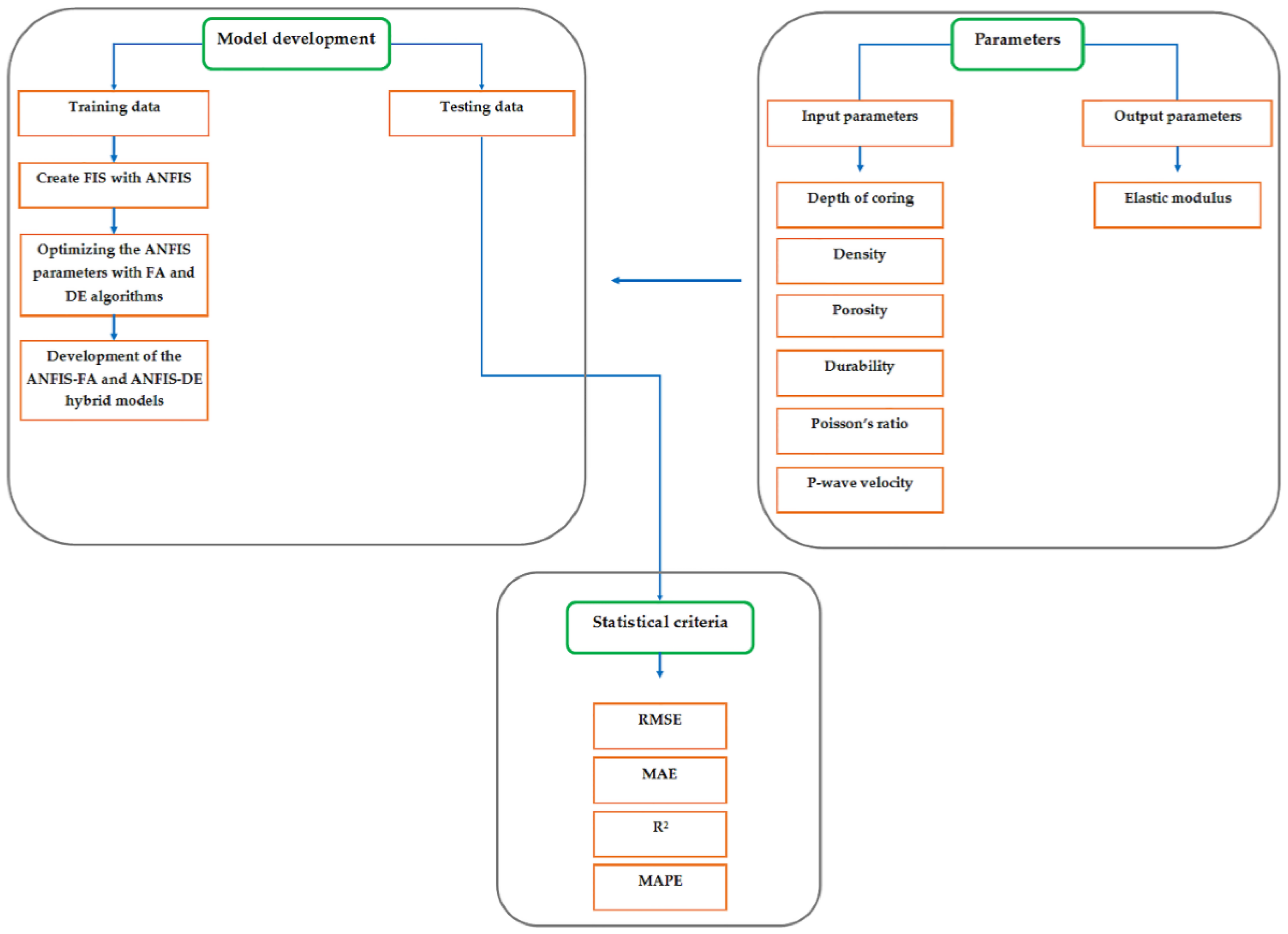
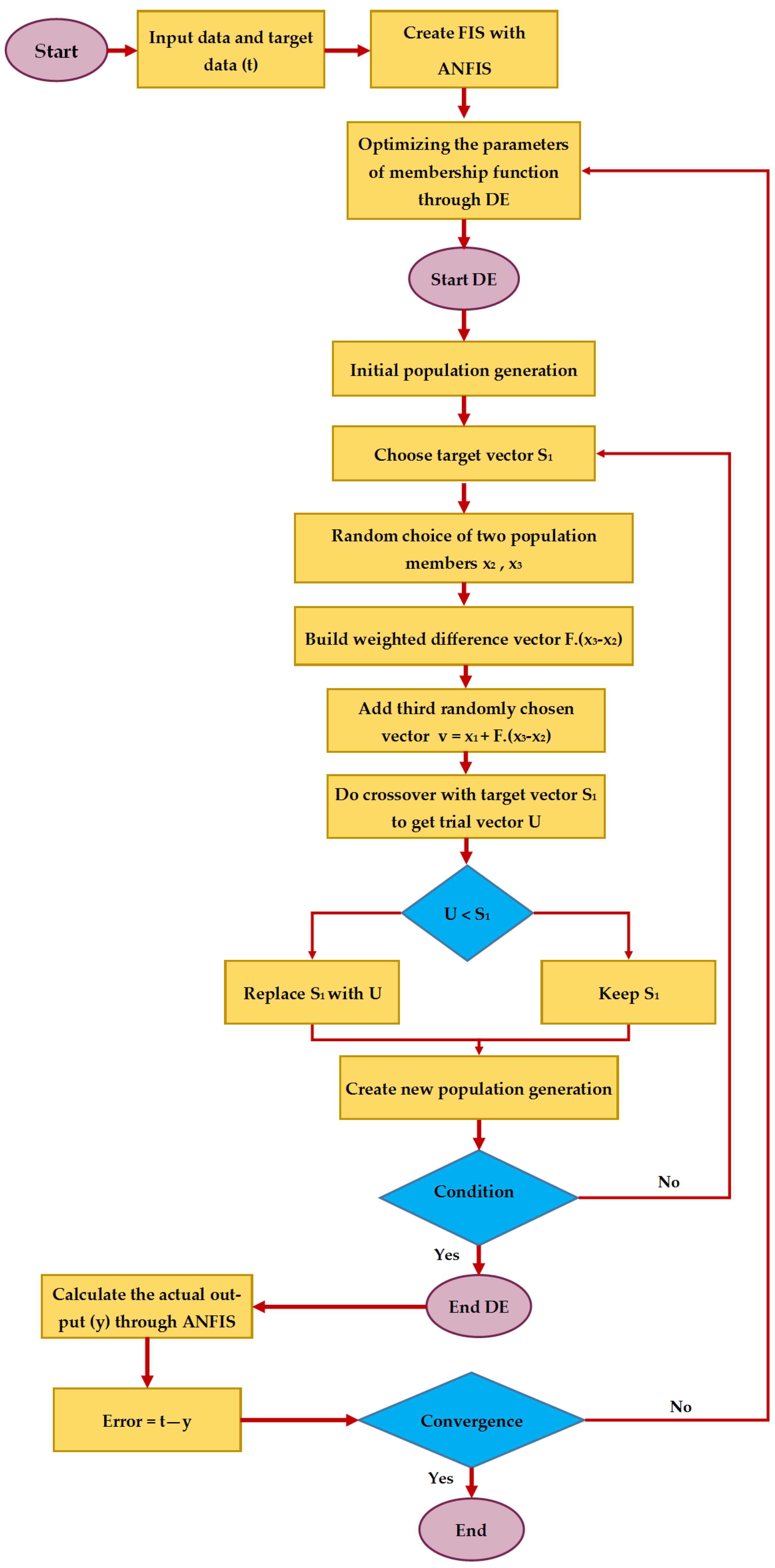
The present study is carried out to assess the potential of applying two hybrid evolutionary models to predict E. The proposed models are based on the integrated expert systems comprising ANFIS with two optimization algorithms, i.e., the firefly algorithm (FA) and differential evolution (DE). To check the effectiveness of FA and DE, the results of ANFIS-FA and ANFIS-DE are then compared with the ANFIS and NN results. The rest of this study is organized as follows. In Section 2, the source of the database is described. Then, the methodologies used in this paper and their implementations are explained in detail in Section 3. Finally, Section 4 and Section 5 present the results/discussions and conclusions of this study, respectively.

2. Source of Database

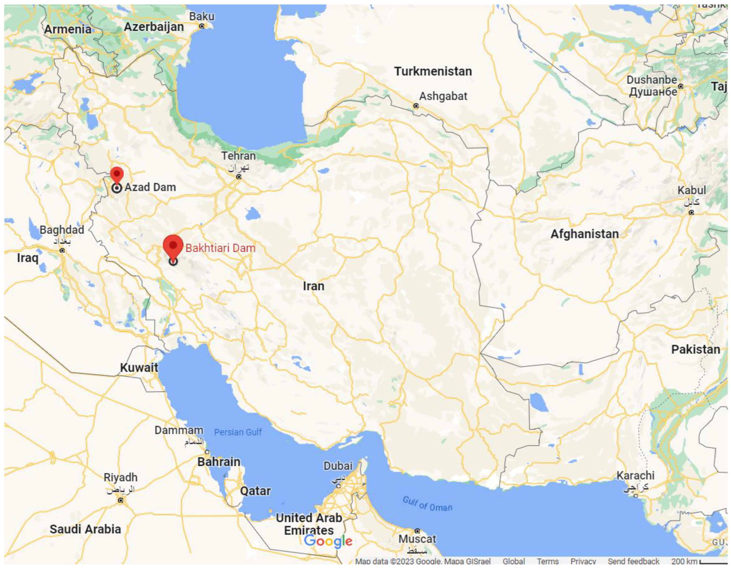
An inclusive database is needed to be formed for E modeling by means of indirect intelligent methods. Such data were obtained through performing laboratory experiments on the core specimens provided from the excavation drilling processes carried out in two under-construction dam sites, namely the Bakhtiari and Azad dams located in Iran. The precise location of the Azad dam site is in the west of Iran, 40 km away from the western city of Sanandaj in the Kurdistan state. It is situated on the Sanandaj–Marivan cities road inside Kurdistan, with the 46°32′57″ to 35°19′59″ geographical coordinates of eastern and northern latitudes, respectively. The construction of this dam is currently in progress. It is mainly aimed at supplying electrical energy and producing power plant storage. The dimensions (length, height, and width) and water storage capacity of this dam are 595 m, 115 m, 11 m, and 260,000,000 m³, respectively.

The Bakhtiari dam is located in the Zagros Highlands, 65 km southwest of the town of Dorud in the Lorestan state, and 70 km northeast of the town of Andimeshk in Khuzestan, Iran. The position of the dam site is at the 48°45′34.87″ to 32°57′23.58″ geographical coordinates of eastern and northern latitudes, respectively (Figure 1). The dam was built upon the Bakhtiari River, aiming to provide adequate water for many purposes, such as drinking, electrical power generation, flood control, and agricultural activities. The dam’s body is at an elevation of 840 m. In addition, in the case of this dam, the peak elevation, crown width, crown length, and foundation width are 325 m, 10 m, 434 m, and 30 m, respectively [20]. The situations of both case studies (the Azad and Bakhtiari dams) on the Iran map are illustrated in Figure 1.

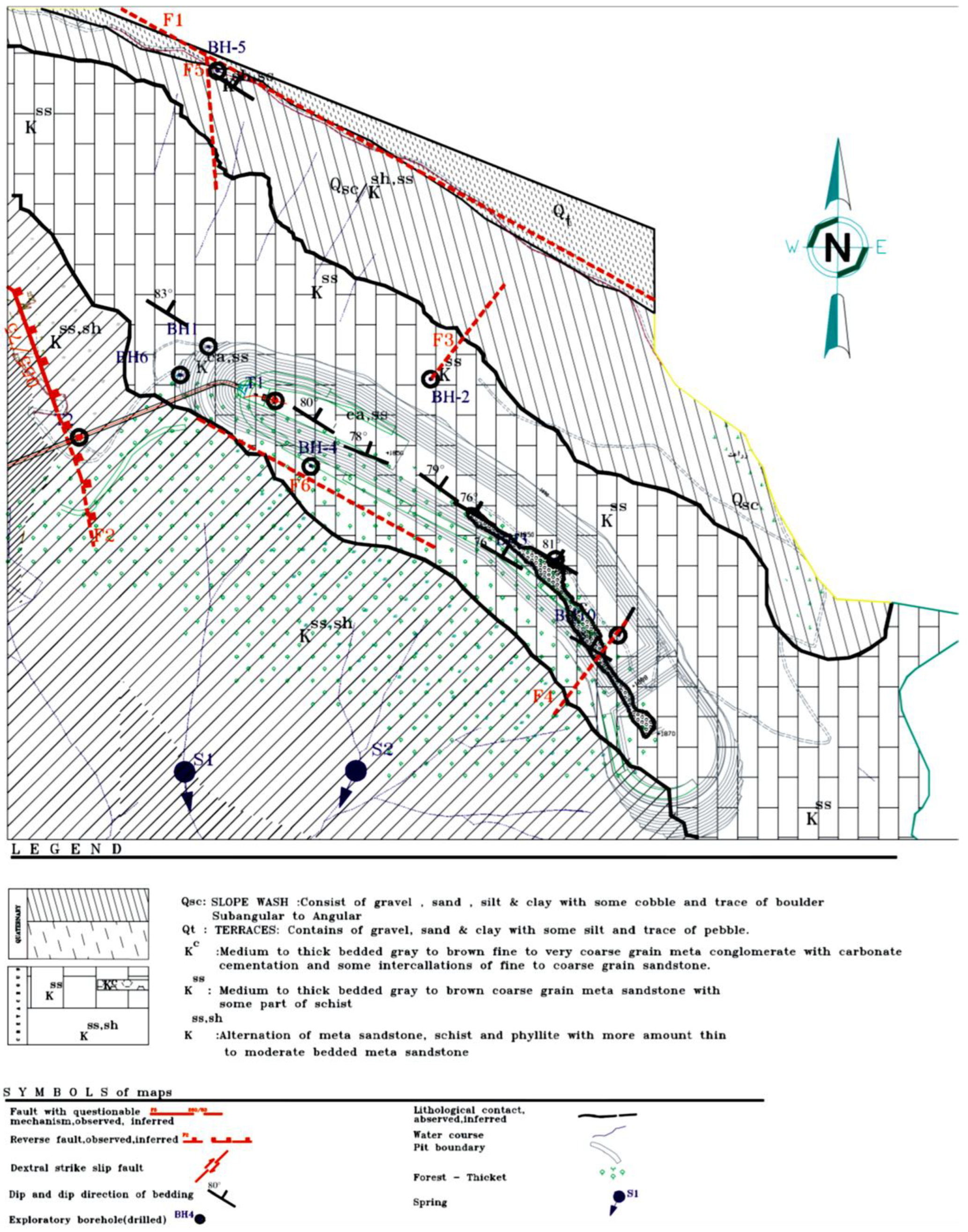
The Azad dam comprises a series of common structures, such as tailraces, higher deposits, different caverns, gurgitation storages, and access tunnels. Geologically, this dam is situated in Iran’s famous formation, Sanandaj–Sirjan, with an alternation of schist, sandstone, limestone, and phylite rocks. The bedrock of the dam mainly comprises sandstone with a low degree of metamorphic, phyllite, and schist. Additionally, within the highland areas, lenses of limestone are also observable. From the stratigraphy point of view, rock outliers from the higher Cretaceous period to the present can be observed within the investigated region. Such rocks consist of four types from the past to the current session: (1) metamorphic rock related to the Cretaceous period that includes a combination of clay and shale; (2) phyllite formation rocks related to the participation of the Cretaceous Paleocene periods, containing limestone and shale with sand; (3) rocks related to the participation of the Paleocene and Eocene periods, comprising sandstone, shale, limestone lenses, and volcanic rocks; and (4) formations related to the Quaternary period, consisting of shallow terraces and debris. From a tectonic viewpoint, the Sarvabad, Kargineh, and Satileh faults are situated 23, 4.5, and 32 km to the south, east, and northeast of the Azad dam, respectively [21]. The geological conditions and faults of the Azad dam site are shown in Figure 2.

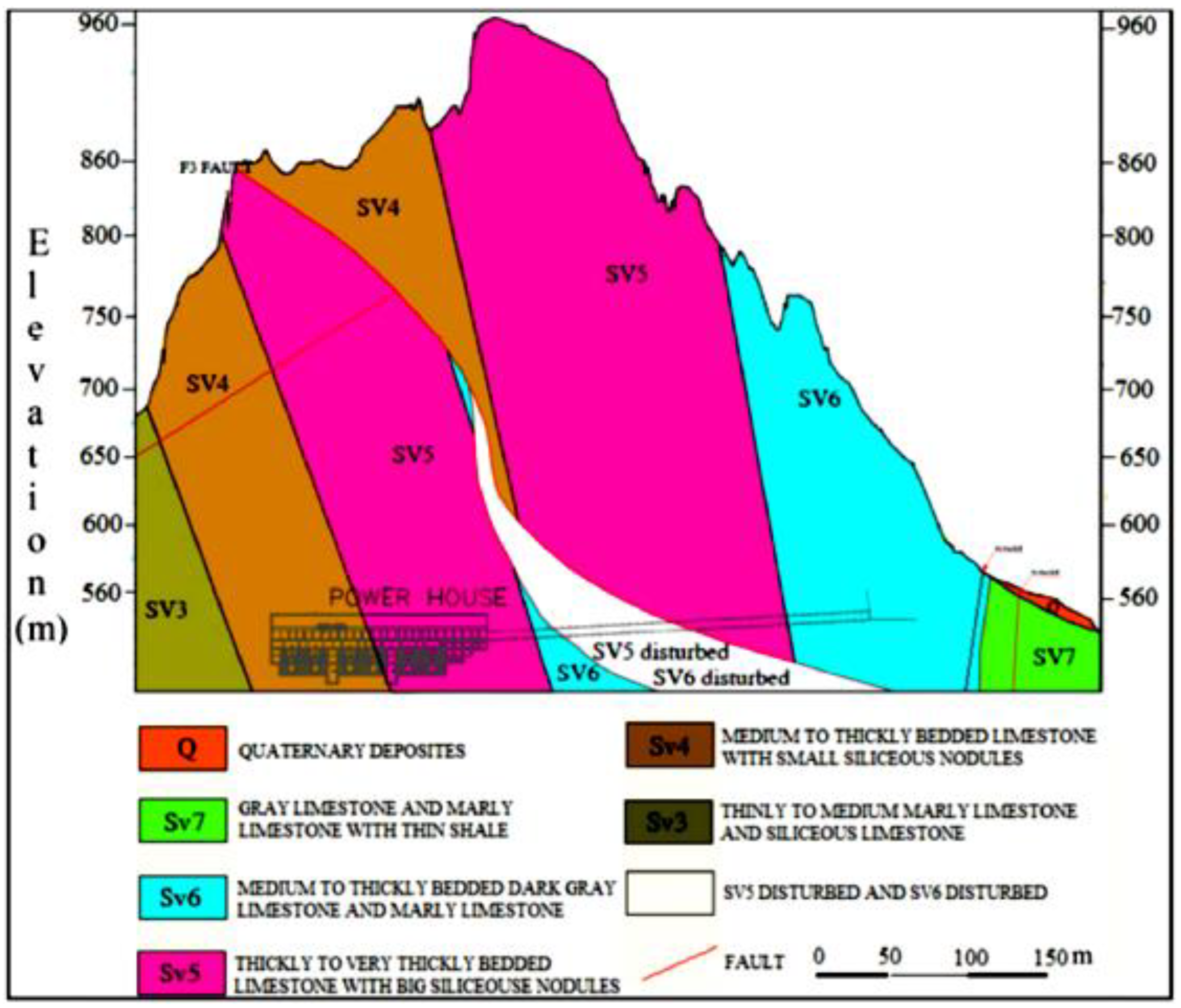
The Bakhtiari dam’s bedrock is made of separate limestone and limestone combined with marl, which incorporates chert nodes. The limestone sections might be synthesized by a combined dolomite substance. From the perspective of geological structure, the dam area is positioned within the pleated Zagros, a portion of the tectono-sediment region of the Zagros. In the lowest northern portion, the area is restricted by pushed Zagros, while in the southwest, it is confined by the Khuzestan plain. With regard to the age of the compressed reservoirs of the area, they date back to between the Triassic and Pliocene eras, and then would have been wrinkled from the Plio-Pleistocene via the latest Alpine organic phase. A number of syncline and anticline sets have been created through such tectonism procedures. Primarily, the above arrangements have been identified by perpendicular axial levels related to the lots of pushed faults in the Zagros area. Additionally, key bed-rocks of the investigated area are made of limestone siliceous related to the current famous formation, Sarvak. This formation (Sarvak) belongs to the Bangestan collection of the middle period of the Cretaceous [20]. For a better review, the geological cross-section of the Bakhtiary dam and plant site is shown in Figure 3.

Database Description

To create inclusive datasets, adequate core samples with NX sizes, i.e., 54 mm in diameter, perpendicular cylindrical shapes, and ratios of height to diameter in the middle of 2:1 to 2.5:1 were used based on the process recommended by the ISRM [22,23]. The samples were arranged from the two dam sites introduced before. When the core specimens were prepared, their various characteristics, such as E value, porosity, density, and durability index, were measured in a laboratory. Furthermore, in the course of the coring operation, each sample’s coring depth was recorded for the purpose of evaluating its impact on the rocks’ geomechanical properties. The laboratory experiments in this study were carried out totally based on the ISRM and ASTM standard methods [22,23]. In this regard, a total of 50 test series were done successfully, and the outputs were documented in the cases of all variables noted above. As a result, 50 datasets were provided, aiming to construct the ANFIS-FA, ANFIS-DE, ANFIS, and NN models. Then, a sorting approach was adopted to divide the available database into training (constructing) and testing datasets. Roughly 20% of the database was determined as the testing dataset in order to be used later in the process of evaluating the models built in this paper.

Note that the ratio of 80 to 20 for training and testing groups has been widely suggested by many scholars, such as Ye et al. [24], Fang et al. [25], Nguyen et al. [26], and Zhou et al. [27]. Aside from that, we also tested the ratio of 70:30. Nevertheless, the 80:20 ratio had better performance; thus, this ratio was used in this study.

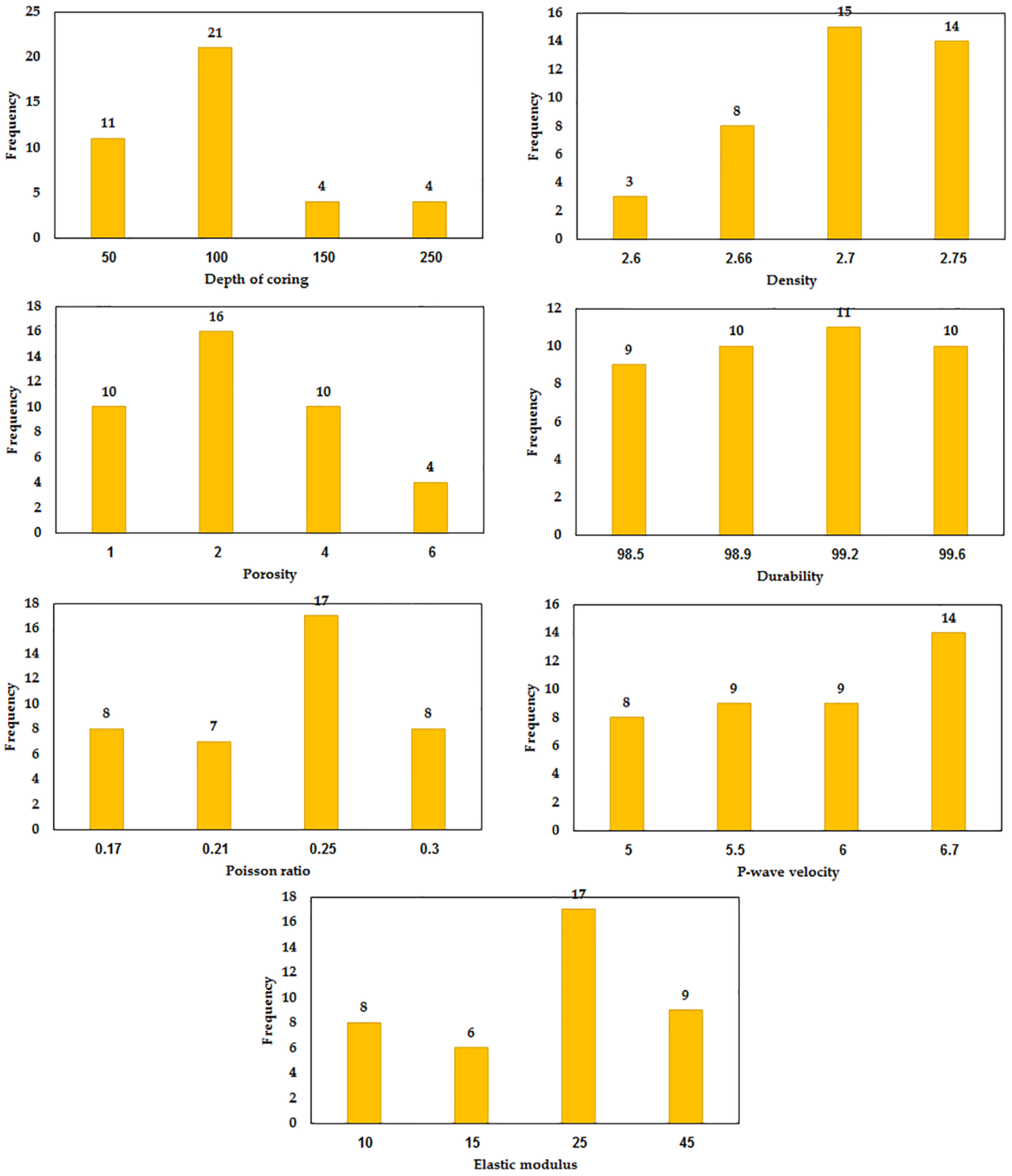
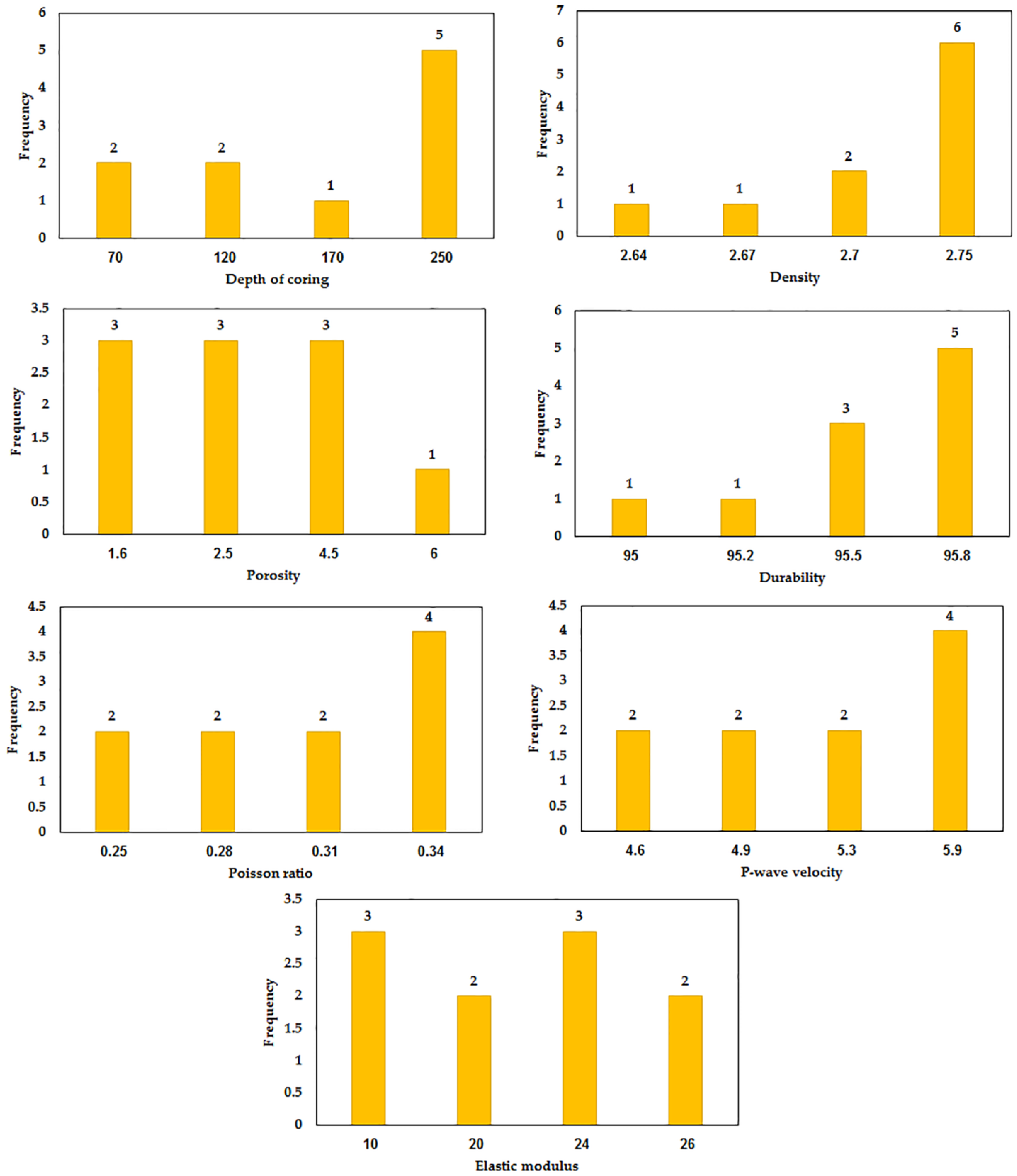
The statistical characteristics of all variables used in this study are shown in

Table 1. Modelling variables and the statistical characteristics datasets.

Statistical Characteristics	Variables
	DC (m)		$\mathit{\rho }$ (g/cm3)		n (%)		DI (%)		ν		Vp (m/s)		E (GPa)
	Train	Test	Train	Test	Train	Test	Train	Test	Train	Test	Train	Test	Train	Test
Mean	79.243	149.455	2.679	2.703	1.992	2.528	98.92	95.45	0.221	0.292	5.564	5.013	18.526	17.586
Standard Error	7.215	21.803	0.007	0.013	0.206	0.429	0.062	0.098	0.007	0.014	0.119	0.145	1.294	2.028
Standard Deviation	45.633	68.948	0.049	0.043	1.305	1.357	0.394	0.310	0.045	0.04	0.756	0.458	8.185	6.413
Sample Variance	2082.38	4753.87	0.002	0.002	1.704	1.842	0.156	0.096	0.002	0.002	0.572	0.210	67.009	41.134
Skewness	1.361	0.051	−1.127	−1.003	1.291	1.795	−0.403	−1.118	0.121	−0.677	−1.258	0.225	0.487	−0.484
Minimum	14	55.85	2.52	2.616	0.37	1.39	98.1	94.8	0.14	0.21	2.985	4.316	3	7.98
Maximum	213.4	248.5	2.74	2.75	5.81	5.81	99.6	95.8	0.3	0.34	6.652	5.82	42.8	25.17

DC: depth of coring, ρ: density, n: porosity, DI: durability, ν: Poisson ratio, Vp: P-wave velocity, E: elastic modulus.

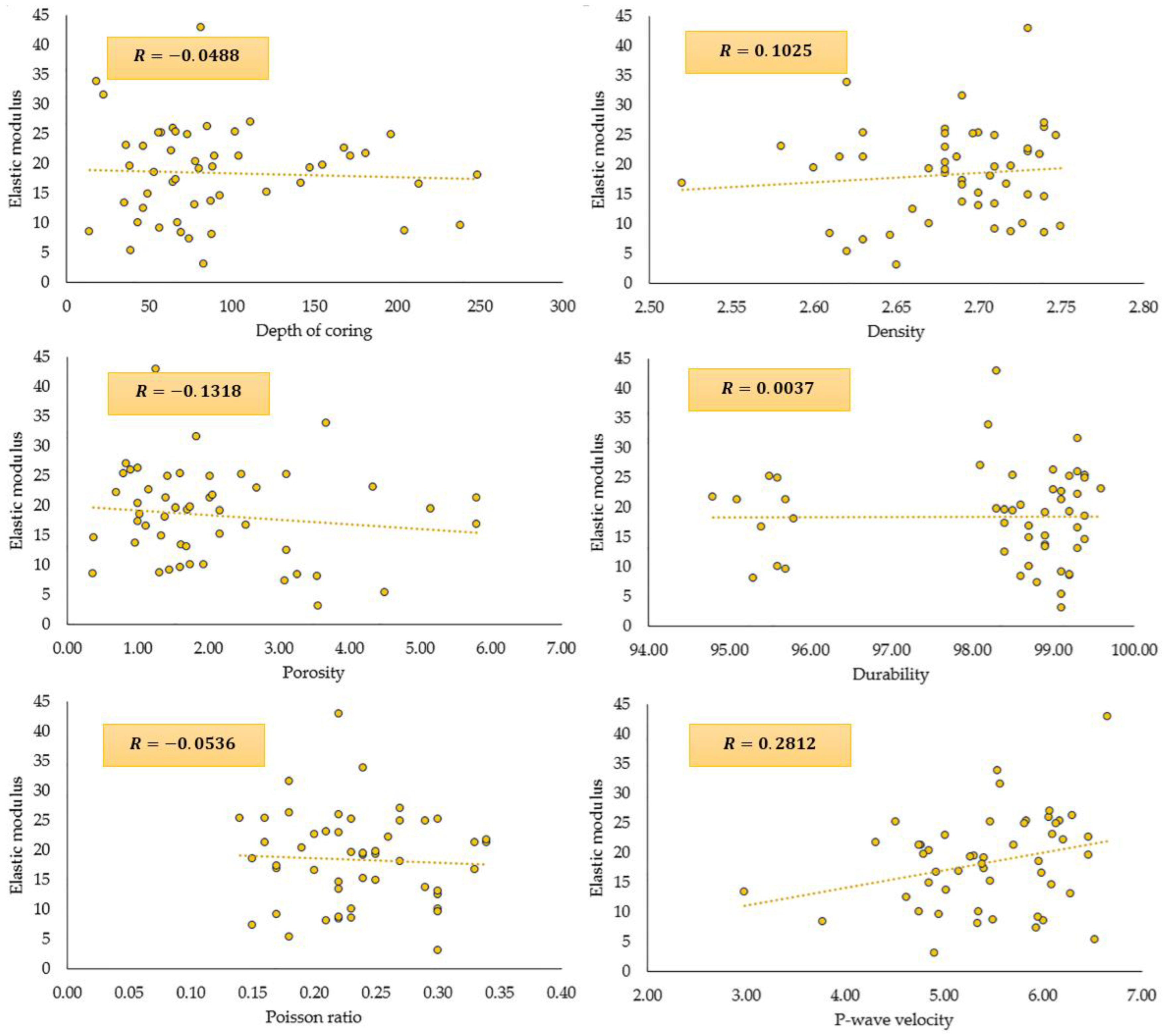
. For a better view, the frequency histogram of all input and output variables are depicted in Figure 4 and Figure 5. For example, in Figure 4, regarding the depth of coring variables, 11, 21, 4, and 4 data were varied in the range of 0–50 m, 50–100 m, 100–150 m, and 150–250 m, respectively. In addition, Figure 6 illustrates the Pearson correlation plots for all variables.

3. Methodology

This section explains how ANFIS combined with the FA and DE algorithms is implemented. Additionally, the modeling process of the NN model is explained in this section. In the aforementioned models, of the total 50 datasets, 40 were used for the training phase and 10 were used for the testing phase. For a better overview, a schematic flowchart of the ANFIS-FA and ANFIS-DE proposed in this study is shown in Figure 7. It is worth mentioning that MATLAB@2018 was used to encode the proposed hybrid models.

3.1. ANFIS Combined with DE

Differential evolution (DE), which was originally proposed by Storn and Price [28], is an effective evolutionary algorithm that works on the basis of a global optimization approach. In general, DE offers three benefits: (1) a simple structure, (2) high-quality solutions achieved, and (3) easy implementation [29]. As a result, it is applied to a variety of conditions. In the present study, DE is used for the aim of minimizing the function of fitness using the amounts of optimized variable. By definition, the function of fitness refers to the root mean square error (RMSE) between the estimated and target datasets. DE, as an innovative algorithm, was implemented in order to adjust the functions of membership amounts of the ANFIS model and, consequently, enhance its overall prediction capability. Figure 4 illustrates the schematic presentation of the hybrid ANFIS-based DE algorithm.

To model ANFIS-DE, four parameters must be specified, namely the number of the iteration, crossover probability, mutation probability, and population size. For the selection of the optimal mutation probability, various values were examined, which can be seen in

Table 2. Selection of the most optimum mutation rate value in implementing the ANFIS-DE model.

Mutation Rate	Performance Criteria		Rank
	R2
	Train	Test
0.05	0.931	0.917	2
0.10	0.942	0.929	5
0.15	0.947	0.923	4
0.20	0.951	0.948	9
0.25	0.946	0.945	8
0.30	0.958	0.952	10
0.35	0.955	0.941	7
0.40	0.948	0.940	6
0.45	0.930	0.925	3
0.50	0.919	0.902	1

. The table also shows that by setting the mutation probability to 0.3, the optimum performance with the highest rank related to the testing phase (i.e., the maximum R² values) was attained. To obtain the best crossover probability, different values were examined (see

Table 3. Selection of the most optimum crossover value in implementing the ANFIS-DE model.

Crossover Rate	Performance Criteria		Rank
	R2
	Train	Test
0.60	0.947	0.932	2
0.65	0.944	0.938	3
0.70	0.953	0.946	5
0.75	0.964	0.961	7
0.80	0.960	0.952	6
0.85	0.943	0.940	4
0.90	0.932	0.927	1

). The table shows that the maximum R² values were attained when the crossover probability was fixed at 0.75. Different population sizes were also tested, as can be observed in

Table 4. Selection of the most optimum population size value in implementing the ANFIS-DE model.

Population Size	Performance Criteria		Rank
	R2
	Train	Test
50	0.929	0.926	1
100	0.935	0.934	2
150	0.948	0.935	3
200	0.964	0.961	9
250	0.976	0.970	10
300	0.975	0.960	8
350	0.969	0.949	6
400	0.955	0.942	5
450	0.957	0.938	4
500	0.951	0.950	7

. The table clearly demonstrates that when the population size was set to 250, the best result (the maximum R² values) was achieved. In these tests, the smallest amount of error was fixed at $1\times {10}^{-5}$, and the peak repetition was set to 500. Accordingly, the crossover probability, mutation probability, and scope of population were fixed to 0.75, 0.3, and 250, respectively. It is worth mentioning that the bolded amounts in Table 2, Table 3 and Table 4 are related to the best results (highest rank) obtained from the developed models.

Figure 8 also shows the ANFIS-DE flowchart used in this study.

3.2. ANFIS Combined with FA

This section introduces a hybridized model combining ANFIS and FA, called ANFIS-FA, with the objective of optimizing the premise parameters of ANFIS. To initiate the modeling process, there is a need to first determine the input-target variables/parameters. When the assembly of the input-target variables/parameters of the model is determined, it is time to determine the training samples. The reason for this is that a model should be capable of predicting the target parameter for those samples that have no effect on the model training process. As a result, the entire dataset was divided into two categories: training/construction and testing/examination samples. As previously mentioned, from among a total of 50 datasets, 20% (n = 10) were chosen in a random way and assigned to the testing group, while the remaining 80% (n = 40) were assigned to the training samples. In addition, it was required to initialize the ANFIS and FA parameters prior to ANFIS modeling in order to predict the target variables. With the use of a trial-and-error-based approach, the optimal amount of membership functions (MFs) was archived as 6. According to the literature [30,31,32], the $\alpha , {\beta }_0, \gamma$, number of variables, and the population are the FA parameters. To improve the ANFIS performance, it was necessary to select the most appropriate values for the aforementioned FA parameters. Table 2 clearly shows that the number of variables is equal to six. As stated in the literature [31,32], in some cases, the value of 1 is suitable for the ${\beta }_0$ parameters. Therefore, in the modelling of ANFIS-FA, the value of ${\beta }_0$ was set to 1.

To select the most appropriate values for the $\alpha \mathrm{and} \gamma$ parameters, various amounts of these parameters were examined, as given in

Table 5. Selection of the optimum $\alpha$ value in implementing the ANFIS-FA.

$\mathit{\alpha }$	Performance Criteria		Rank
	R2
	Train	Test
0.10	0.945	0.933	1
0.20	0.947	0.941	4
0.30	0.954	0.943	5
0.40	0.951	0.948	6
0.50	0.958	0.955	8
0.60	0.962	0.956	9
0.70	0.951	0.949	7
0.80	0.944	0.938	2
0.90	0.941	0.940	3

and

Table 6. Selection of the optimum $\gamma$ value in implementing the ANFIS-FA.

$\mathit{\gamma }$	Performance Criteria		Rank
	R2
	Train	Test
0.5	0.951	0.947	1
1	0.959	0.955	3
1.5	0.973	0.968	6
2	0.971	0.960	5
2.5	0.965	0.958	4
3	0.952	0.951	2

. Considering these tables, the most appropriate values (the highest R²) for the $\alpha \mathrm{and} \gamma$ parameters were obtained with $\alpha =0.6$ and $\gamma =1.5$. As a result, the values of 0.6 and 1.5 were used for the $\alpha \mathrm{and} \gamma$ parameters in ANFIS-FA modelling. By setting the number of iterations to 1000, different values were also tested to select the most appropriate value for the population size, as shown in

Table 7. Selection of the optimum population value in implementing the ANFIS-FA.

Population	Performance Criteria		Rank
	R2
	Train	Test
50	0.965	0.961	4
100	0.972	0.966	6
150	0.973	0.971	7
200	0.979	0.975	8
250	0.971	0.965	5
300	0.963	0.960	3
350	0.958	0.957	2
400	0.955	0.948	1

. The table shows that the best performance was attained with population = 200. Based on the above descriptions, the values of 6, 1, 0.6, 1.5 and 200 were set as the number of variables, ${\beta }_0$, $\alpha , \gamma$, and population size, respectively. It is worth mentioning that the bolded amounts in Table 5, Table 6 and Table 7 are related to the best results (highest rank) obtained from the developed models. In this step, the most appropriate value of the number of iterations needed to be determined. According to the results, after the 15th iteration, no significant change was observed in the ANFIS-FA performance. In other words, after 15 iterations, the performance for different populations was constant. Accordingly, the number of iterations in ANFIS-FA modelling used in this study was set to 15. When the user-based defined parameters in the investigated models (FA and ANFIS) were determined, then the ANFIS training process was begun with the use of the training samples. To this end, the FA algorithm was used to optimize the primary part of the fuzzy If-Then rules, and the least-square method was applied to the optimization of the linear consequent fuzzy rules.

Additionally, the preliminary light strength corresponding to the primary generation was computed, and then each firefly’s attractiveness level was measured. With the use of the movement equation, those fireflies that had a lower level of attraction were pushed toward the brighter firefly. Afterward, the light strength and individual firefly’s position were updated, and the function of fitness was computed again. All steps involved in ANFIS-FA are displayed in Figure 9.

3.3. Neural Network (NN)

Neural Networks (NNs), especially the Multi-Layer Perceptron (MLP), are widely used in prediction models applied to different engineering problems [31,32]. MLP, which is employed in the present study, contains three layers: input, hidden, and output layers. Therefore, as can be seen in Figure 6, the nodes that exist within the input layer correspond to DC, $\rho$, n, DI, ν, and Vp, while those in the output layer correspond to E. Based on the trial-and-error approach, we considered the number of nodes within the hidden layer. The evaluation results showed that the existence of seven nodes within the hidden layer can result in a higher reliability. As can be observed in Figure 10, the hidden layer with seven nodes resulted in the optimal performance of NN (with the maximum R²). It is worth mentioning that, to select the suitable number of nodes inside the hidden layer, different numbers were tested. As a result, the NN structure in the present research was built on the basis of six nodes within the first/input layer, seven nodes within the second/hidden layer, and one node within the last/output layer.

4. Results and Discussion

The present study was aimed at examining the effectiveness of the FA and DE algorithms in optimizing ANFIS for the prediction of E. The results obtained from the proposed ANFIS-FA and ANFIS-DE models were compared to those of ANFIS and NN models. Here, the models’ prediction capabilities were assessed regarding RMSE, mean of average percentage error (MAPE), mean of absolute error (MAE), variance account for (VAF), A10-index, and performance index (PI) [33,34,35,36,37], as presented in the following equations:

$$\mathrm{MAE}=\frac{1}{n}{{\displaystyle \sum }}_{i=1}^n\left|A_i-P_i\right|$$

(1)

$$\mathrm{RMSE}=\sqrt{\frac{{{\displaystyle \sum }}_{i=1}^n{(A_i-P_i)}^2}{n}}$$

(2)

$$\mathrm{MAPE}=\left[\frac{1}{n}{{\displaystyle \sum }}_{i=1}^n\frac{\left|A_i-P_i\right|}{A_m}\right]\times 100$$

(3)

$$\mathrm{VAF}=\left[1-\frac{var \left(A_i-P_i\right)}{var \left(A_i\right)}\right]\times 100$$

(4)

$$A10-index=\frac{m10}{n}$$

(5)

$$PI=\frac{1}{\overline{A_i}}\frac{RMSE}{R+1}$$

(6)

where n stands for the number of data (n = 50), and $A_i$, $P_i$, and $\overline{A_i}$ signify the actual, estimated, and average of actual E values, respectively. Additionally, m10 is the number of data with values of rate actual/predicted values (ranging from 0.9 to 1.1), and R in Equation (6) is the correlation coefficient.

Table 8. Performance of the models to predict E by using six statistical criteria.

Model	Statistical Criteria												Total Rank
	RMSE		MAE		MAPE (%)		VAF (%)		A10-Index		PI
	Train; Rank	Test; Rank	Train; Rank	Test; Rank	Train; Rank	Test; Rank	Train; Rank	Test; Rank	Train; Rank	Test; Rank	Train; Rank	Test; Rank	Train	Test
ANFIS	2.337; 2	2.557; 2	2.258; 2	2.456; 2	10.173; 2	13.965; 2	93.274; 2	92.514; 2	0.35; 2	0.4; 2	0.064; 2	0.070; 2	12	12
NN	2.491; 1	2.781; 1	2.409; 1	2.639; 1	10.849; 1	15.006; 1	92.341; 1	90.985; 1	0.3; 1	0.4; 2	0.068; 1	0.076; 1	6	7
ANFIS-DE	1.447; 3	1.827; 3	1.384; 3	1.662; 3	6.236; 3	9.451; 3	97.436; 3	96.957; 3	0.75; 3	0.6; 3	0.039; 3	0.049; 3	18	18
ANFIS-FA	0.909; 4	1.152; 4	0.865; 4	1.100; 4	3.899; 4	6.254; 4	98.962; 4	98.778; 4	0.925; 4	0.9; 4	0.024; 4	0.031; 4	24	24

presents the MAPE (%), MAE, RMSE, VAF(%), and A10-Index values attained by the developed models.

As can be observed in Table 8, the lowest MAPE (%), MAE, RMSE, and PI values were determined for the ANFIS-FA model as 6.254%, 1.1, 1.152, and 0.031, respectively. In addition, the highest VAF (%) and A10-index values were determined for the ANFIS-FA model as 98.778% and 0.9, respectively. These values were calculated for the ANFIS-DE model as 1.827, 1.662, 9.452%, 0.049, 96.957%, and 0.6, respectively; for the ANFIS model as 2.557, 2.456, 13.965%, 0.070, 92.514%, and 0.4, respectively; and for the NN model as 2.781, 2.639, 15.006%, 0.076, 90.985%, and 0.4, respectively. According to Table 8, the highest total rank values for both the training and testing groups were obtained by the ANFIS-FA model. 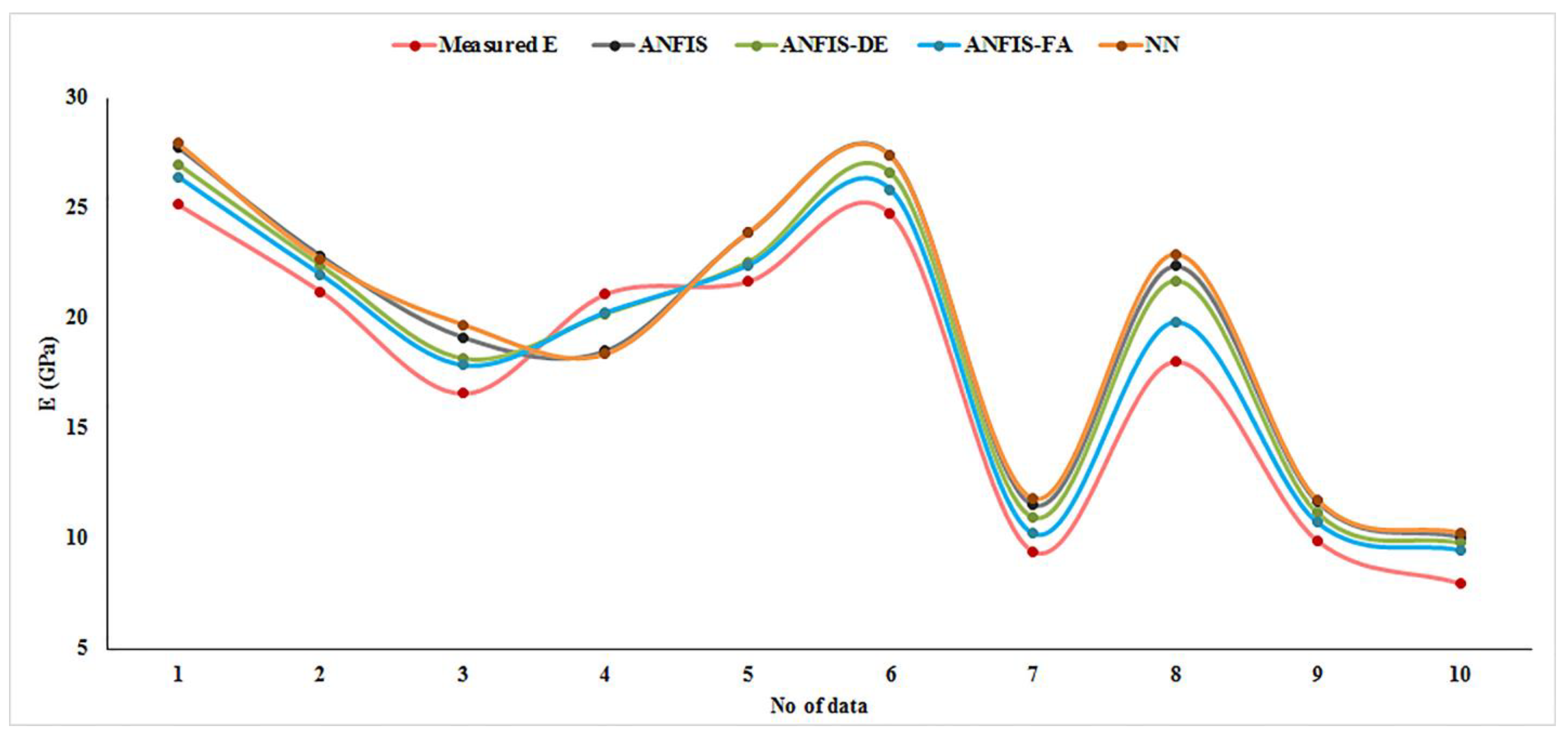It is worth mentioning that the bolded amounts in Table 8 are related to the best results (highest rank) obtained from the ANFIS-FA model. 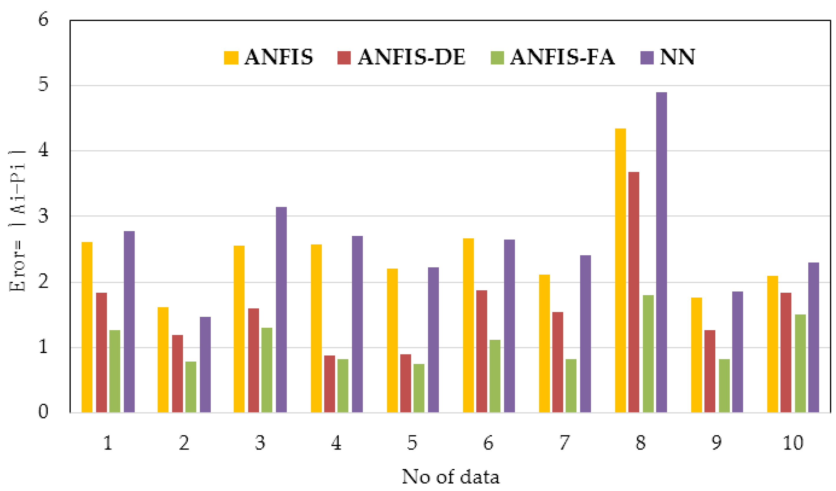For a better overview, the predicted E values provided by all models in the testing phase are depicted in Figure 11. Additionally, Figure 12 shows the amount of error for each model related to the testing phase. According to these two figures, the prediction of E by the ANFIS-FA model is very accurate and closer to measured E values. 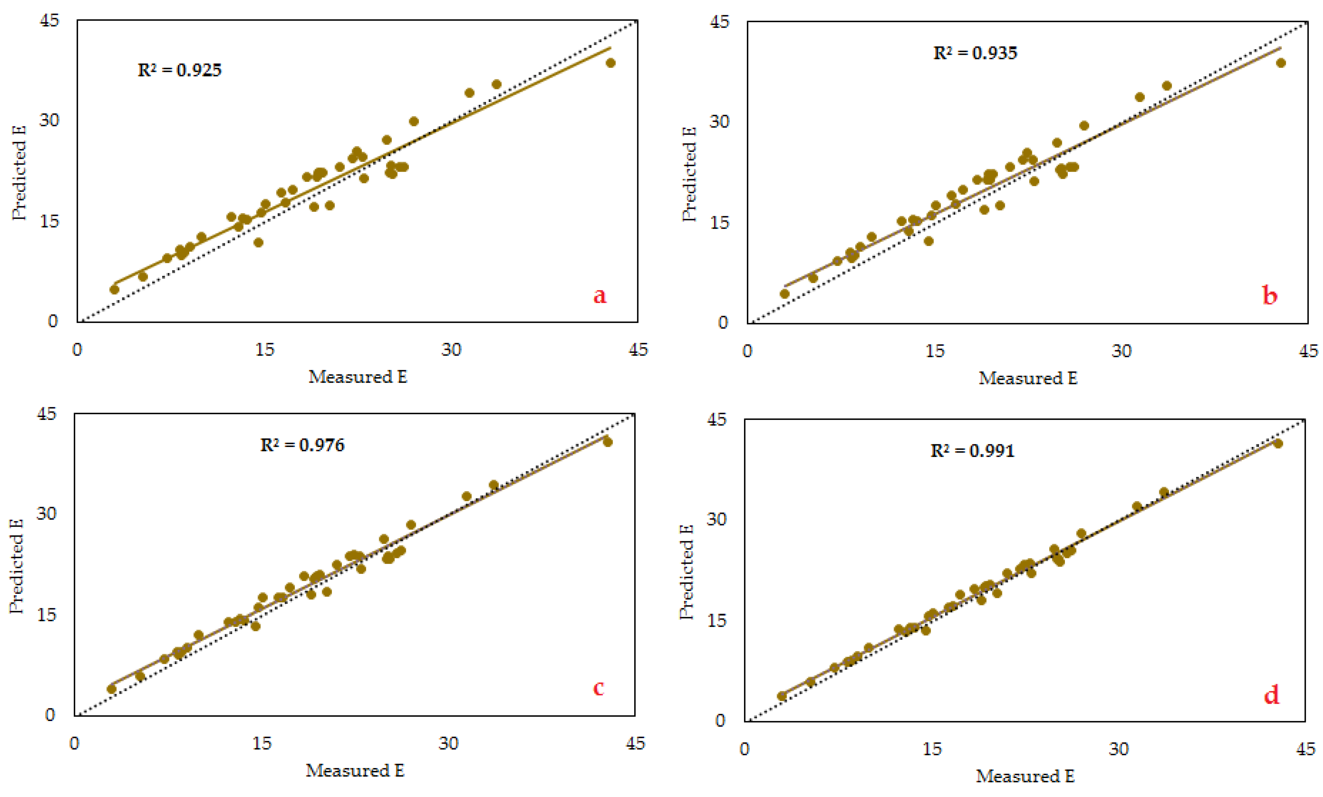In addition, Figure 13 and Figure 14 demonstrate the scatter plots of actual versus estimated E values with the use of all predictive models. The figures show that the ANFIS-FA model obtained a greater value for the coefficients of determination (R²). The R² values of 0.988, 0.970, 0.928, and 0.913 were obtained by the ANFIS-FA, ANFIS-DE, ANFIS, and NN models, respectively. Accordingly, FA was more effective in comparison with DE in regard to the ANFIS improvement. 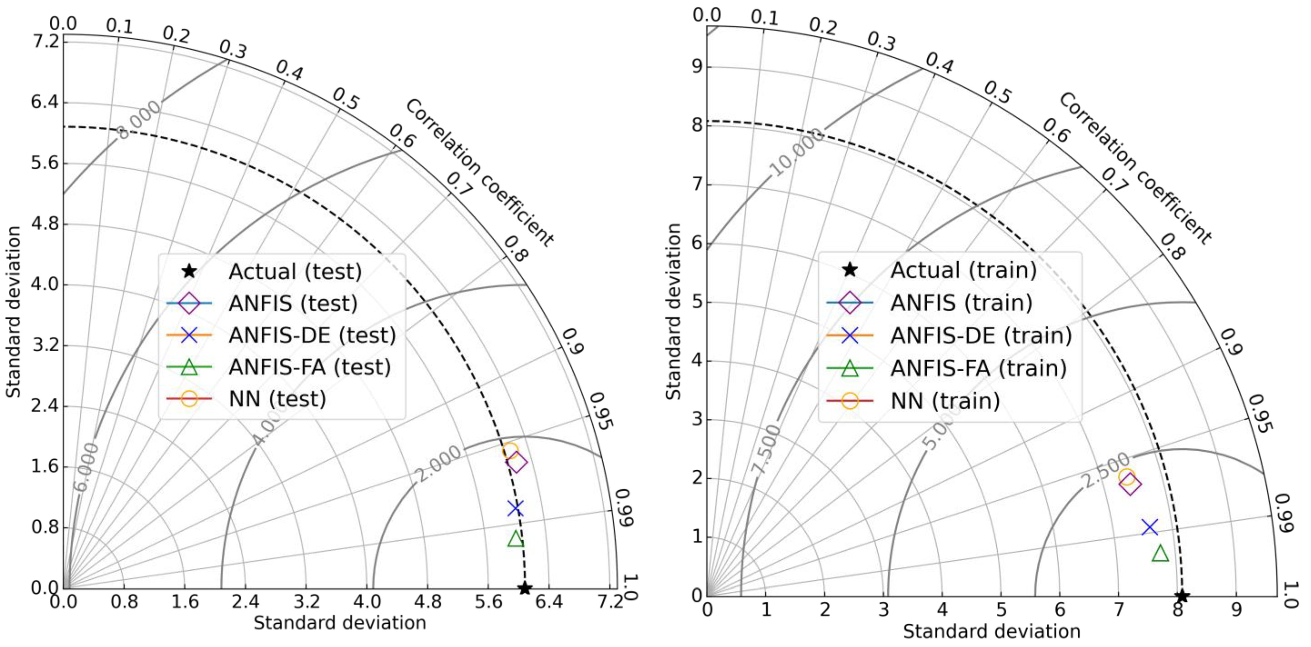Furthermore, the absolute error of ANFIS-FA, ANFIS-DE, ANFIS, and NN models in predicting E for testing datasets (ten datasets) is depicted in Figure 15. According to this Figure, the orange-coloured line, which was obtained by the ANFIS-FA model, yields the lowest absolute error for all ten datasets. 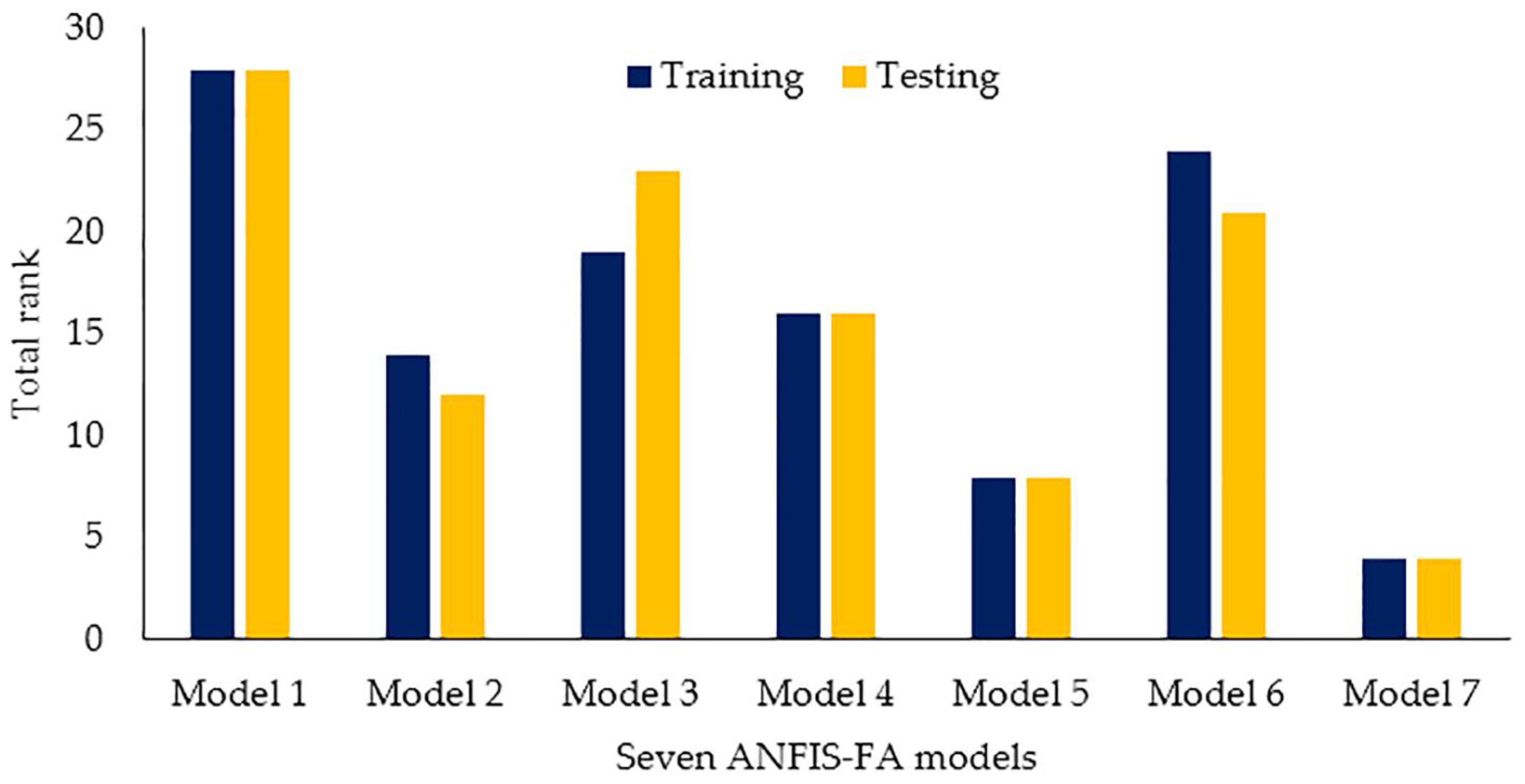Moreover, the Taylor diagrams for both training and testing groups are shown in Figure 16. The results show that the ANFIS-FA has a stronger potential to predict E than the others. In this study, a sensitivity analysis was also performed. For this work, the effect of removing each input variable on E for the ANFIS-FA was calculated. In this regard, six new models based on the combination of input variables were constructed, as follows:

• Model 1: inputs: all variables given in Table 1.
• Model 2: inputs: all variables given in Table 1 except the depth of coring.
• Model 3: inputs: all variables given in Table 1 except density.
• Model 4: inputs: all variables given in Table 1 except porosity.
• Model 5: inputs: all variables given in Table 1 except durability.
• Model 6: inputs: all variables given in Table 1 except Poisson ratio.
• Model 7: inputs: all variables given in Table 1 except P-wave velocity.

Figure 11. Comparing the values of E predicted by the four models.

Figure 11. Comparing the values of E predicted by the four models.

Figure 12. Amount of error for each model, as related to the testing phase.

Figure 12. Amount of error for each model, as related to the testing phase.

Figure 13. Comparison of the actual E value with those predicted, obtained by (a) NN, (b) ANFIS, (c) ANFIS-DE, and (d) ANFIS-FA for the training group.

Figure 13. Comparison of the actual E value with those predicted, obtained by (a) NN, (b) ANFIS, (c) ANFIS-DE, and (d) ANFIS-FA for the training group.

Figure 14. Comparison of the actual E value with those predicted, obtained by (a) NN, (b) ANFIS, (c) ANFIS-DE, and (d) ANFIS-FA for the testing group.

Figure 14. Comparison of the actual E value with those predicted, obtained by (a) NN, (b) ANFIS, (c) ANFIS-DE, and (d) ANFIS-FA for the testing group.

Figure 15. Absolute error values obtained by the models using the testing phase.

Figure 15. Absolute error values obtained by the models using the testing phase.

Figure 16. Taylor diagrams obtained by the predictive models.

Figure 16. Taylor diagrams obtained by the predictive models.

The results of the above models are presented in

Table 9. Performance of all seven ANFIS-FA models.

Model	Statistical Criteria								Total Rank
	RMSE		MAE		MAPE (%)		VAF (%)
	Train; Rank	Test; Rank	Train; Rank	Test; Rank	Train; Rank	Test; Rank	Train; Rank	Test; Rank	Train	Test
Model 1	0.909; 7	1.152; 7	0.865; 7	1.100; 7	3.899; 7	6.254; 7	98.962; 7	98.778; 7	28	28
Model 2	1.776; 3	2.306; 3	1.683; 4	2.204; 3	7.583; 4	12.532; 3	95.979; 3	95.848; 3	14	12
Model 3	1.570; 4	1.523; 6	1.508; 5	1.460; 6	6.790; 5	8.30; 6	96.910; 5	96.50; 5	19	23
Model 4	1.739; 5	2.056; 4	1.695; 3	2.022; 4	7.635; 4	11.497; 4	96.673; 4	96.254; 4	16	16
Model 5	1.856; 2	2.447; 2	1.808; 2	2.386; 2	8.146; 2	13.567; 2	95.899; 2	95.321; 2	8	8
Model 6	1.524; 6	1.917; 5	1.441; 6	1.838; 5	6.493; 6	10.451; 5	97.353; 6	96.808; 6	24	21
Model 7	2.279; 1	3.054; 1	2.167; 1	2.986; 1	9.761; 1	16.979; 1	93.408; 1	92.691; 1	4	4

, which shows that models 1 and 7 had the highest total rank (i.e., the best performance) and lowest total rank (i.e., the worst performance), respectively (Figure 17). Note that, the results of model 1 is bolded in Table 9. The results of presented in Table 9 indicated that once the P-wave velocity was removed from the modeling, the worst performance was obtained; thus, P-wave velocity can be determined as the most effective variable in the modeling.

5. Conclusions

The elastic modulus (E) is considered one of the most significant factors in the primary and ultimate plans of projects related to the geo-engineering field. As a result, it is highly necessary to predict E with a high accuracy level. This paper examined the use of two hybrid evolutionary models, namely ANFIS-FA and ANFIS-DE, to predict E. Additionally, the traditional ANFIS and NN models were developed for comparison aims. In total, 50 datasets were collected during the drilling process in the Azad and Bakhtiari under-construction dams in Iran. Out of the 50 datasets, 40 were used to construct the models, and the remaining datasets were used to test them. The input parameters considered in the construction of the models were porosity, density, depth of coring, Poisson’s ratio, compressional/primary wave velocity, and durability, which were assigned as the input variables, whereas E was the output/target variable. Finally, some statistical indices were designed in order to demonstrate the capacity of the models in the prediction of E. According to the findings, the following results and remarks can be briefly listed:

• The results demonstrated that ANFIS-FA was the most suitable model for the prediction of E in the cases studied. The ANFIS-DE, ANFIS, and NN models were identified as the next cases in this rank.
• The FA and DE algorithms strongly improved the ANFIS performance in terms of predicting the E value. This confirms the effectiveness of FA and DE; accordingly, these two algorithms can be effectively used to address other predicting problems in rock engineering fields.
• The results of sensitivity analysis showed that the P-wave velocity was the most effective parameter on the intensity of E.
• For future studies in this field, other evolutionary algorithms, e.g., the central force optimization, chicken swarm optimization, elephant search algorithm, and flower pollination algorithm, could be implemented to enhance the ANFIS performance.

References

1. Ocak, I.; Evren Seker, S. Estimation of Elastic Modulus of Intact Rocks by Artificial Neural Network. Rock Mech. Rock Eng. 2012, 45, 1047–1054. [Google Scholar] [CrossRef]
2. Jahed Armaghani, D.; Mohamad, E.T.; Momeni, E.; Monjezi, M.; Narayanasamy, M.S. Prediction of the strength and elasticity modulus of granite through an expert artificial neural network. Arab. J. Geosci. 2016, 9, 48. [Google Scholar] [CrossRef]
3. Sachpazis, C.I. Correlating Schmidt hardness with compressive strength and Young’s modulus of carbonate rocks. Int. Assoc. Eng. Geol. Bull. 1990, 42, 75–83. [Google Scholar] [CrossRef]
4. Karakus, M.; Kumral, M.; Kilic, O. Predicting elastic properties of intact rocks from index tests using multiple regression modelling. Int. J. Rock Mech. Min. Sci. 2005, 42, 323–330. [Google Scholar] [CrossRef]
5. Sonmez, H.; Gekceoglu, C.; Nefeslioglu, H.A.; Kayabasi, A. Estimation of rock modulus for intact rocks with an artificial neural network and for rock masses with a new empirical equation. Int. J. Rock Mech. Min. Sci. 2006, 43, 224–235. [Google Scholar] [CrossRef]
6. Katz, O.; Reches, Z.; Roegiers, J.C. Evaluation of mechanical rock properties using Schmidt hammer. Int. J. Rock Mech. Min. Sci. 2000, 37, 723–728. [Google Scholar] [CrossRef]
7. Kilic, A.; Teymen, A. Determination of mechanical properties of rocks using simple methods. Bull. Eng. Geol. Environ. 2008, 67, 237–244. [Google Scholar] [CrossRef]
8. Yagiz, S. Correlation between slake durability and rock properties for some carbonate rocks. Bull. Eng. Geol. Environ. 2011, 70, 377–383. [Google Scholar] [CrossRef]
9. Nefeslioglu, H.A. Evaluation of geo-mechanical properties of very weak and weak rock materials by using non-destructive techniques: Ultrasonic pulse velocity measurements and reflectance spectroscopy. Eng. Geol. 2013, 160, 8–20. [Google Scholar] [CrossRef]
10. Singh, R.; Kainthola, A.; Singh, T.N. Estimation of elastic constant of rocks using an ANFIS approach. Appl. Soft Comput. 2012, 12, 40–45. [Google Scholar] [CrossRef]
11. Beiki, M.; Majdi, A.; Dadi Givshad, A. Application of genetic programming to predict the uniaxial compressive strength and elastic modulus of carbonate rocks. Int. J. Rock Mech. Min. Sci. 2013, 63, 159–169. [Google Scholar] [CrossRef]
12. Feng, X.; Jimenez, R. Bayesian prediction of elastic modulus of intact rocks using their uniaxial compressive strength. Eng. Geol. 2014, 173, 32–40. [Google Scholar] [CrossRef]
13. Ghasemi, E.; Kalhori, H.; Bagherpour, R.; Yagiz, S. Model tree approach for predicting uniaxial compressive strength and Young’s modulus of carbonate rocks. Bull. Eng. Geol. Environ. 2018, 77, 331–343. [Google Scholar] [CrossRef]
14. Jahed Armaghani, D.; Mohamad, E.T.; Momeni, E.; Narayanasamy, M.S.; Amin, M.F.M. An adaptive neuro-fuzzy inference system for predicting unconfined compressive strength and Young’s modulus: A study on Main Range granite. Bull. Eng. Geol. Environ. 2015, 74, 1301–1319. [Google Scholar] [CrossRef]
15. Rezaei, M. Indirect measurement of the elastic modulus of intact rocks using the Mamdani fuzzy inference system. Measurement 2018, 129, 319–331. [Google Scholar] [CrossRef]
16. Rezaei, M. Feasibility of novel techniques to predict the elastic modulus of rocks based on the laboratory data. Int. J. Geotech. Eng. 2020, 14, 25–34. [Google Scholar] [CrossRef]
17. Sarkhani Benemaran, R.; Esmaeili-Falak, M.; Javadi, A. Predicting resilient modulus of flexible pavement foundation using extreme gradient boosting based optimised models. Int. J. Pavement Eng. 2022, 1–20. [Google Scholar] [CrossRef]
18. Shahani, N.M.; Zheng, X.; Guo, X.; Wei, X. Machine Learning-Based Intelligent Prediction of Elastic Modulus of Rocks at Thar Coalfield. Sustainability 2022, 14, 3689. [Google Scholar] [CrossRef]
19. Tsang, L.; He, B.; Rashid, A.S.A.; Jalil, A.T.; Sabri, M.M.S. Predicting the Young’s Modulus of Rock Material Based on Petrographic and Rock Index Tests Using Boosting and Bagging Intelligence Techniques. Appl. Sci. 2022, 12, 10258. [Google Scholar] [CrossRef]
20. Asadizadeh, M.; Hossaini, M.F. Predicting rock mass deformation modulus by artificial intelligence approach based on dilatometer tests. Arab J. Geosci. 2016, 9, 96. [Google Scholar] [CrossRef]
21. Rezaei, M. Forecasting the stress concentration coefficient around the mined panel using soft computing methodology. Eng. Comput. 2019, 35, 451–466. [Google Scholar] [CrossRef]
22. ASTM. Soil and Rock, Annual Book of ASTM Standards; ASTM International: West Conshohocken, PA, USA, 2002; Volume 4.08. [Google Scholar]
23. ISRM. Rock Characterization Testing and Monitoring, ISRM Suggested Methods; Pergamon Press: Oxford, UK, 1981. [Google Scholar]
24. Ye, J.; Koopialipoor, M.; Zhou, J.; Armaghani, D.J.; He, X. A Novel Combination of Tree-Based Modeling and Monte Carlo Simulation for Assessing Risk Levels of Flyrock Induced by Mine Blasting. Nat. Resour. Res. 2021, 30, 225–243. [Google Scholar] [CrossRef]
25. Fang, Q.; Nguyen, H.; Bui, X.N.; Tran, Q.H. Estimation of Blast-Induced Air Overpressure in Quarry Mines Using Cubist-Based Genetic Algorithm. Nat. Resour. Res. 2020, 29, 593–607. [Google Scholar] [CrossRef]
26. Nguyen, H.; Bui, X.N.; Bui, H.B.; Mai, N.L. Correction to: A comparative study of artificial neural networks in predicting blast-induced air-blast overpressure at Deo Nai open-pit coal mine, Vietnam. Neural. Comput. Appl. 2021, 33, 10615. [Google Scholar] [CrossRef]
27. Zhou, J.; Li, C.; Koopialipoor, M.; Jahed Armaghani, D.; Pham, B.T. Development of a new methodology for estimating the amount of PPV in surface mines based on prediction and probabilistic models (GEP-MC). Int. J. Min. Reclam. Environ. 2021, 35, 48–68. [Google Scholar] [CrossRef]
28. Storn, R.; Price, K. Differential evolution–a simple and efficient heuristic for global optimization over continuous spaces. J. Glob. Optim. 1997, 11, 341–359. [Google Scholar] [CrossRef]
29. Bui, D.T.; Pradhan, B.; Nampak, H.; Bui, Q.T.; Tran, Q.A.; Nguyen, Q.P. Hybrid artificial intelligence approach based on neural fuzzy inference model and metaheuristic optimization for flood susceptibilitgy modeling in a high-frequency tropical cyclone area using GIS. J. Hydrol. 2016, 540, 317–330. [Google Scholar] [CrossRef]
30. Shang, Y.; Nguyen, H.; Bui, X.N.; Tran, Q.H.; Moayedi, H. A Novel Artificial Intelligence Approach to Predict Blast-Induced Ground Vibration in Open-Pit Mines Based on the Firefly Algorithm and Artificial Neural Network. Nat. Resour. Res. 2020, 29, 723–737. [Google Scholar] [CrossRef]
31. Cao, J.; Gao, J.; Nikafshan Rad, H.; Mohammed, A.S.; Hasanipanah, M.; Zhou, J. A novel systematic and evolved approach based on XGBoost-firefly algorithm to predict Young’s modulus and unconfined compressive strength of rock. Eng. Comput. 2022, 38, 3829–3845. [Google Scholar] [CrossRef]
32. Zhou, J.; Li, C.; Arslan, C.H.; Hasanipanah, M.; Bakhshandeh Amnieh, H. Performance evaluation of hybrid FFA-ANFIS and GA-ANFIS models to predict particle size distribution of a muck-pile after blasting. Eng. Comput. 2021, 37, 265–274. [Google Scholar] [CrossRef]
33. Hasanipanah, M.; Monjezi, M.; Shahnazar, A.; Jahed Armaghanid, D.; Farazmand, A. Feasibility of indirect determination of blast induced ground vibration based on support vector machine. Measurement 2015, 75, 289–297. [Google Scholar] [CrossRef]
34. He, B.; Armaghani, D.J.; Lai, S.H. Assessment of tunnel blasting-induced overbreak: A novel metaheuristic-based random forest approach. Tunn. Undergr. Space Technol. 2023, 133, 104979. [Google Scholar] [CrossRef]
35. Ghanizadeh, A.R.; Ghanizadeh, A.; Asteris, P.G.; Fakharian, P.; Armaghani, D.J. Developing Bearing Capacity Model for Geogrid-Reinforced Stone Columns Improved Soft Clay utilizing MARS-EBS Hybrid Method. Transp. Geotech. 2022, 38, 100906. [Google Scholar] [CrossRef]
36. Ashrafian, A.; Taheri Amiri, M.J.; Rezaie-Balf, M.; Ozbakkaloglu, T.; Lotfi-Omran, O. Prediction of compressive strength and ultrasonic pulse velocity of fiber reinforced concrete incorporating nano silica using heuristic regression methods. Constr. Build. Mater. 2018, 190, 479–494. [Google Scholar] [CrossRef]
37. Armaghani, D.J.; Asteris, P.G. A comparative study of ANN and ANFIS models for the prediction of cement-based mortar materials compressive strength. Neural Comput. Appl. 2021, 33, 4501–4532. [Google Scholar] [CrossRef]
Figure 1. Situations of both case studies (the Azad and Bakhtiari Dams).
Sustainability 15 04230 g001
Figure 2. Geological conditions of the Azad dam site [15].
Sustainability 15 04230 g002
Figure 3. Geological cross-section of the Bakhtiary dam and plant site [15].
Sustainability 15 04230 g003
Figure 4. Frequency histogram of all variables for the training group.
Sustainability 15 04230 g004
Figure 5. Frequency histogram of all variables for the testing group.
Sustainability 15 04230 g005
Figure 6. Pearson correlation plots for all input variables vs. the output (E).
Sustainability 15 04230 g006
Figure 7. A schematic flowchart of the ANFIS-FA and ANFIS-DE proposed in this study.
Sustainability 15 04230 g007
Figure 8. ANFIS-DE Flowchart.
Sustainability 15 04230 g008
Figure 9. Implementing the ANFIS-FA used in this study.
Sustainability 15 04230 g009
Figure 10. Use of various numbers of nodes in the second/hidden layer with their R2 values.
Sustainability 15 04230 g010
Figure 17. Total ranks of all seven constructed ANFIS-FA models to evaluate the sensitivity analysis.
Sustainability 15 04230 g017