

Analyzing Geotechnical Characteristics of Soils in Erbil via GIS and ANNs

Abstract
:1. Introduction
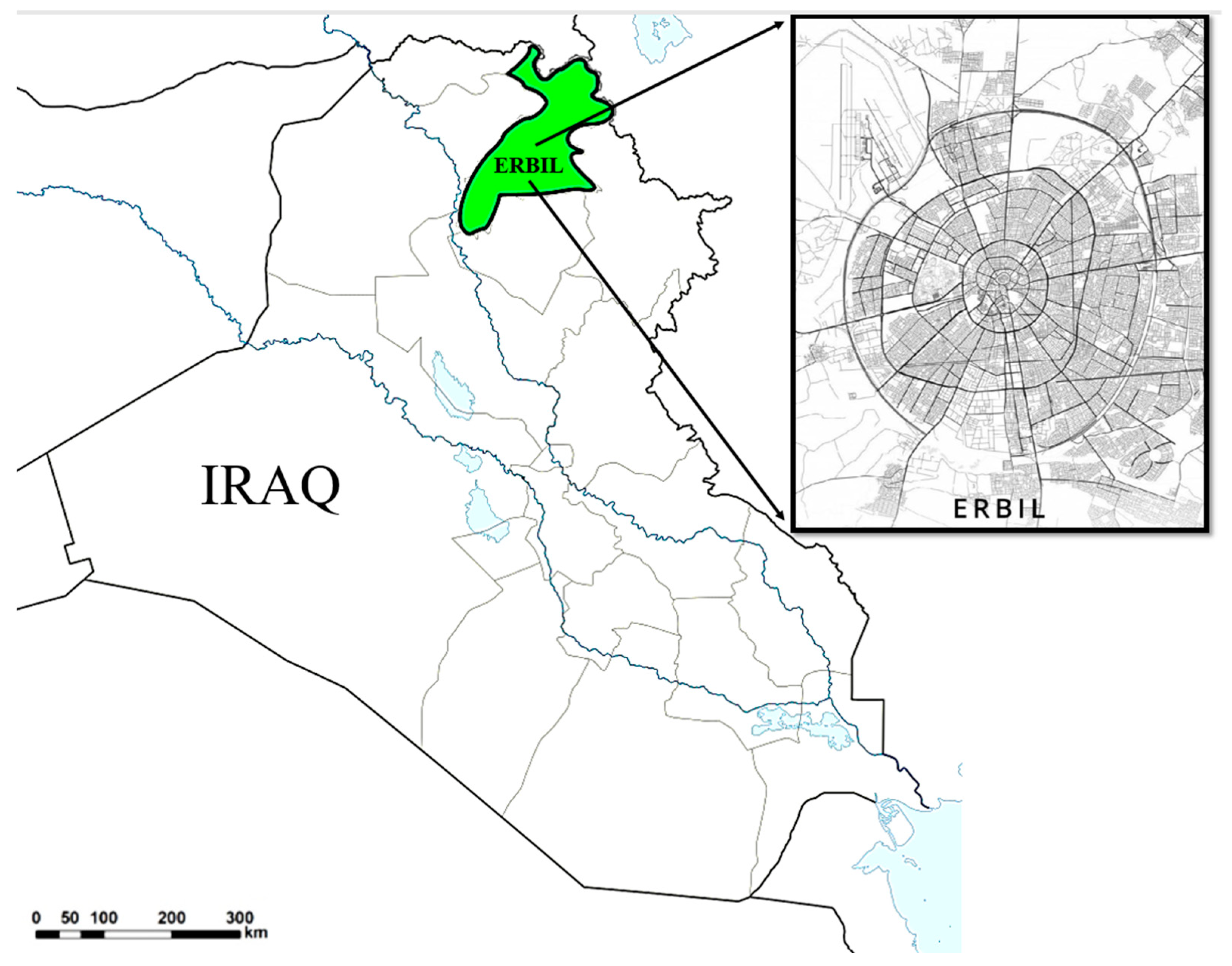
2. Study Area
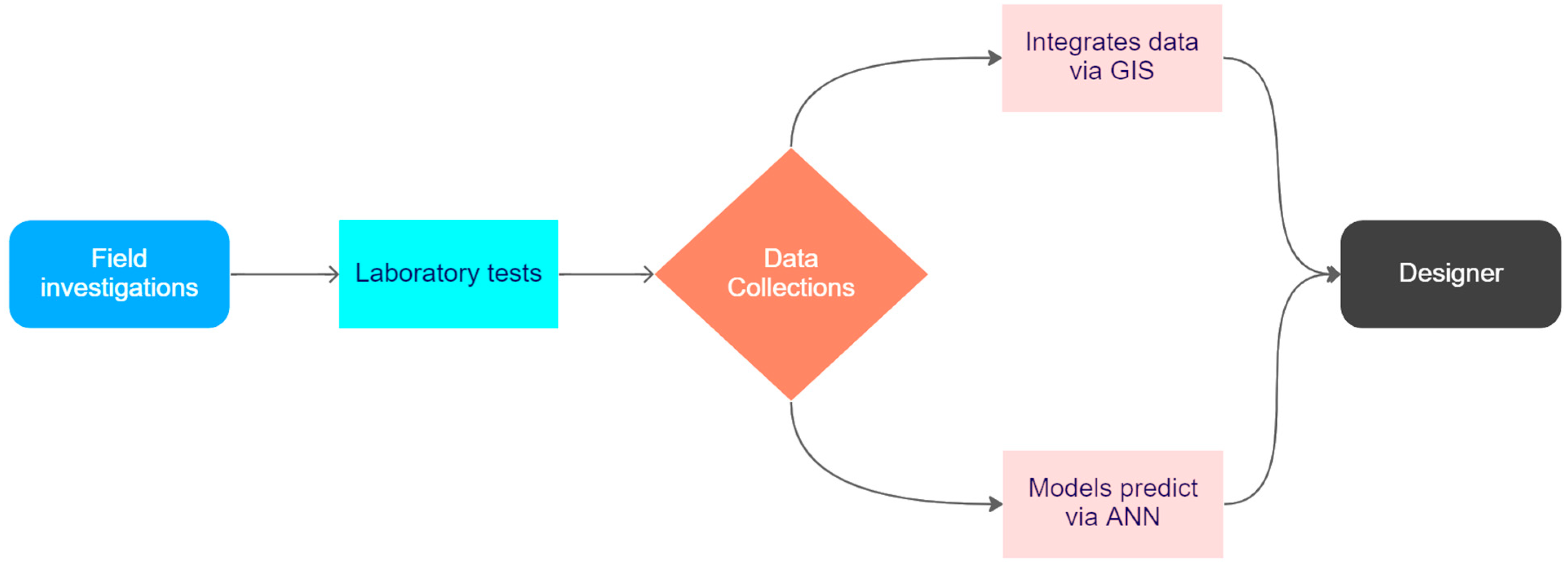
3. Methodology
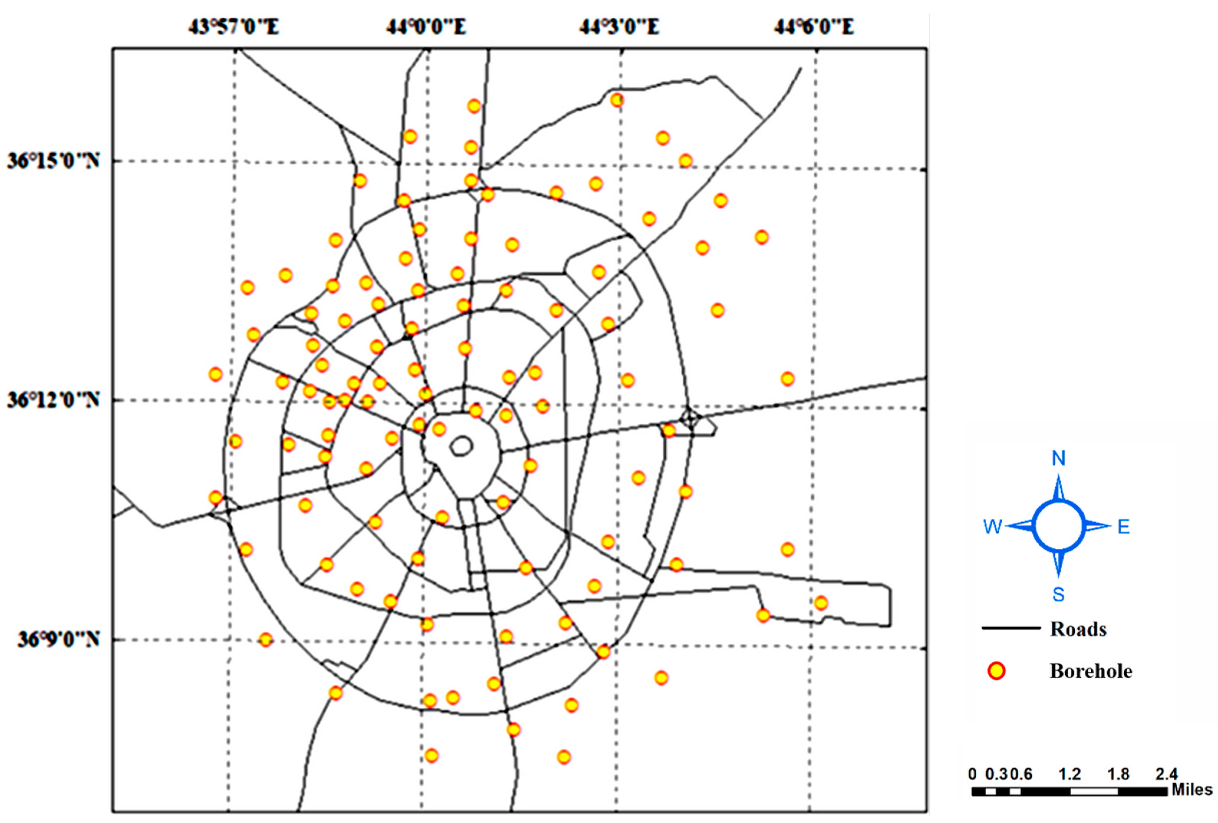
3.1. Data Collection
3.2. Geographical Information Systems (GISs)
- Interpolation: This method is used to predict values at unsampled locations based on observed data. Interpolation methods in ArcGIS include inverse distance weighting, spline, and triangulated irregular network (TIN) interpolation.
- Buffering: This method is used to create a polygon around a feature that represents a specified distance. Buffers are commonly used in spatial analysis to identify areas that are within a certain distance of a feature of interest.
- Overlay: This method is used to combine two or more maps based on a set of rules or conditions. Overlays can be used to create a new map that shows the spatial relationships between features in the input maps.
- Reclassification: This method is used to change the values of a raster or vector layer based on a set of rules or conditions. Reclassification is often used to simplify complex data or to create new data layers based on existing data.
- Extraction: This method is used to select features from a map based on a set of conditions or rules. Extractions can be used to create new data layers that contain only the features that meet specific criteria [11].
3.3. Statistical Analysis
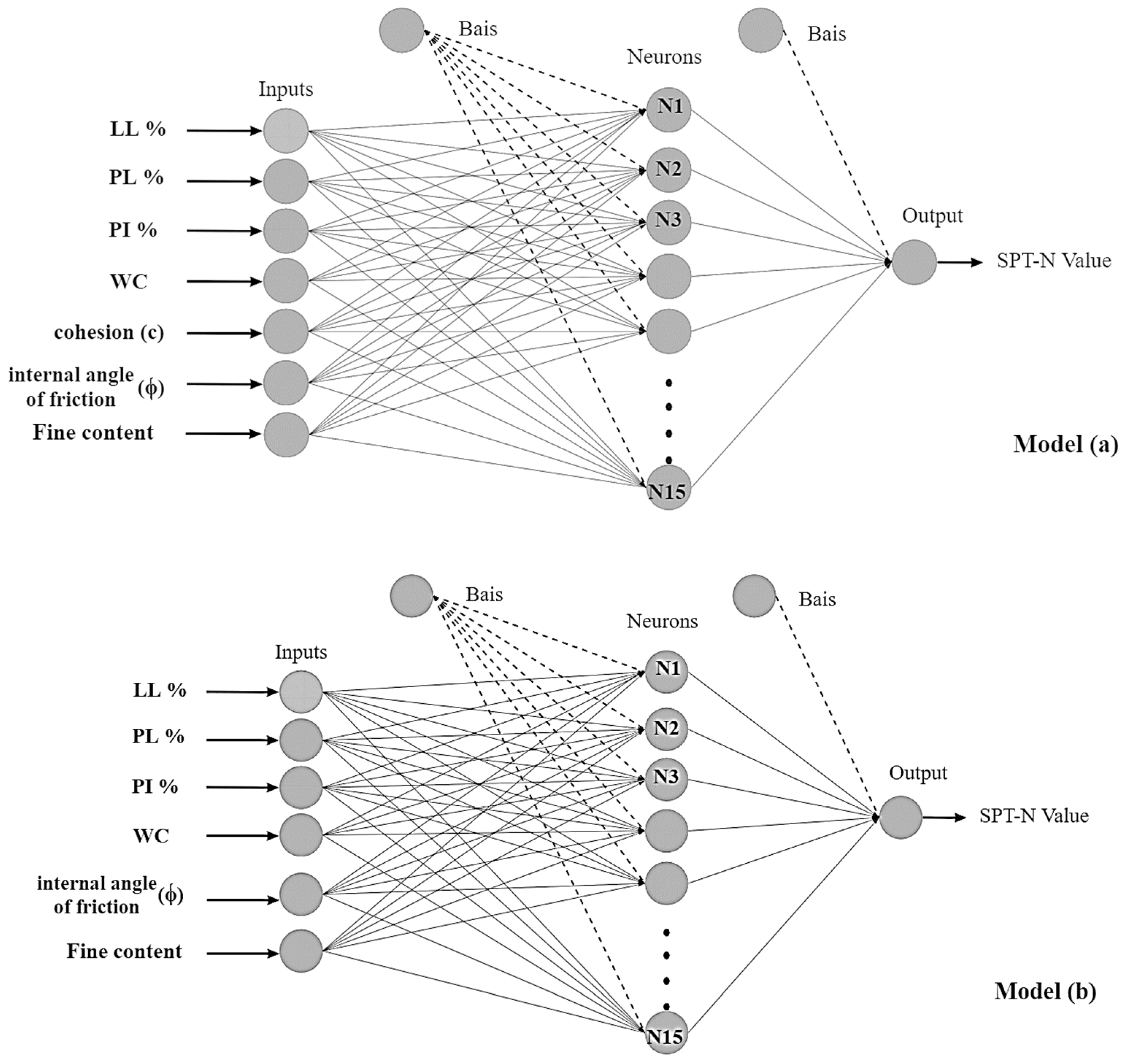
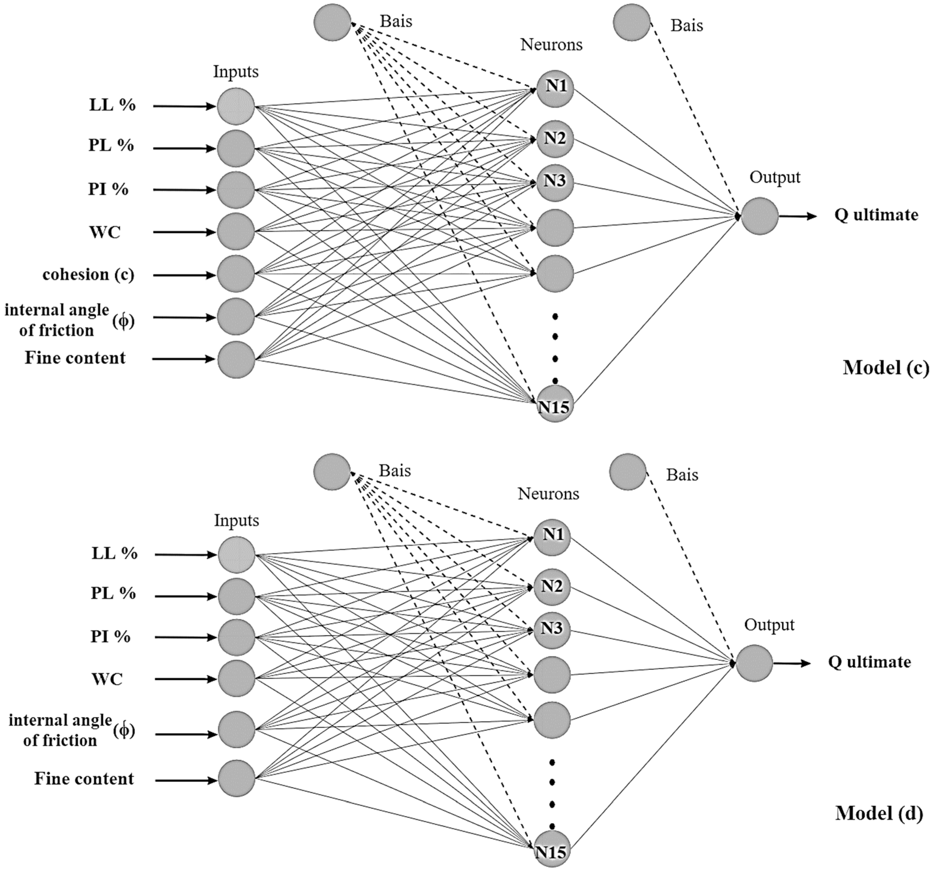
3.4. Neural Network Model
4. Results and Discussions
4.1. Modeling of Soil Properties Using GIS Maps
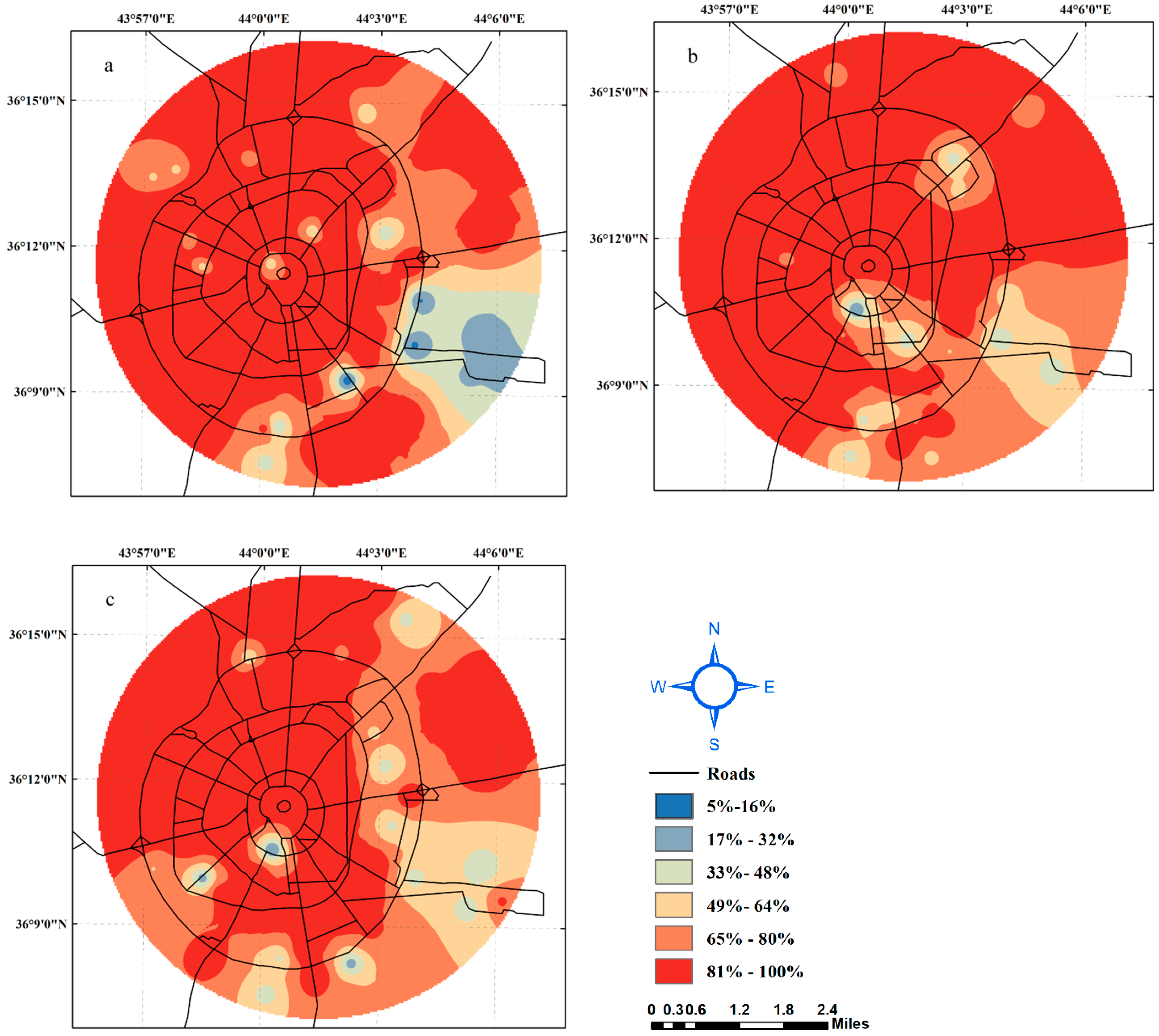
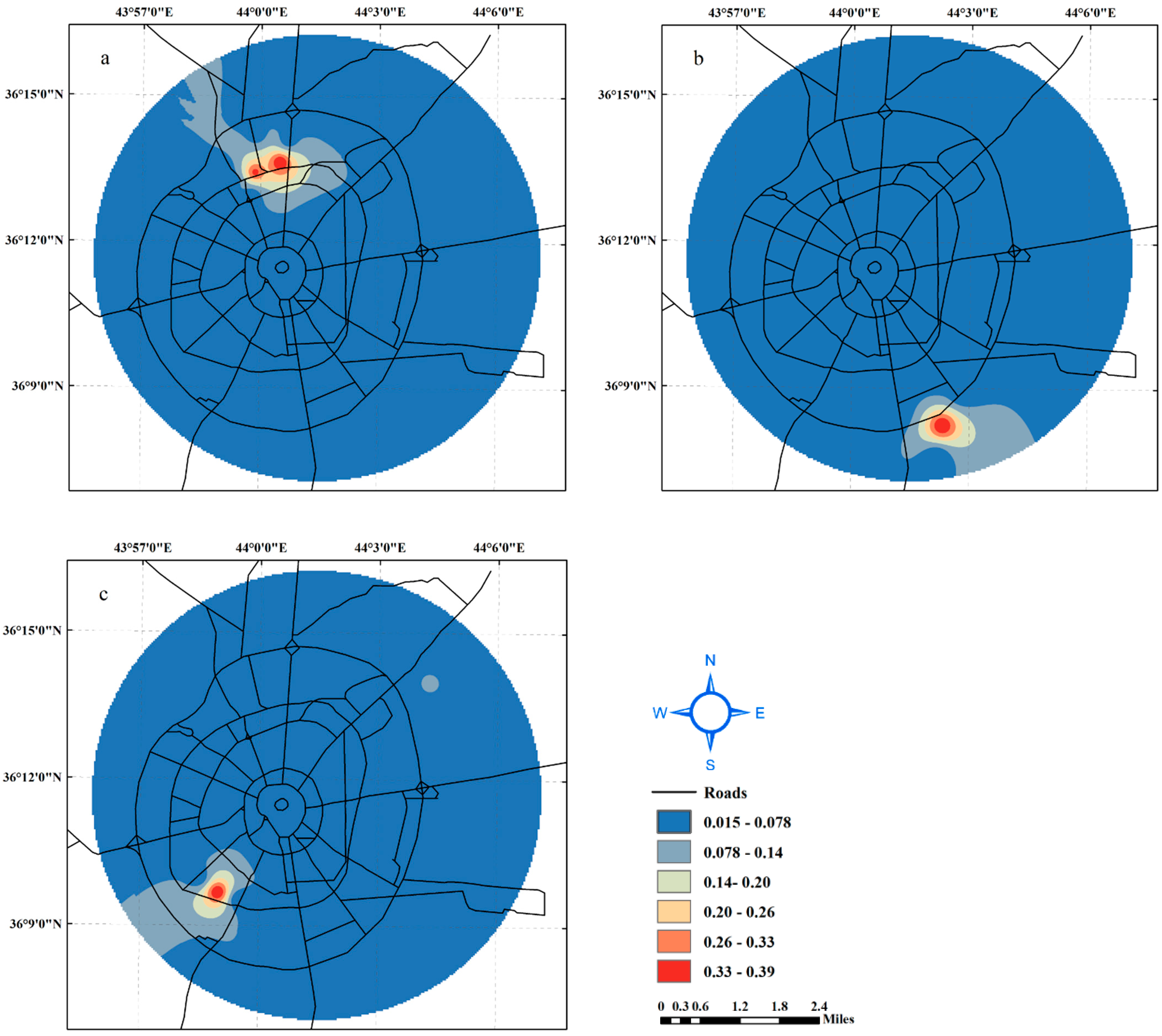
4.1.1. Fines Content Model
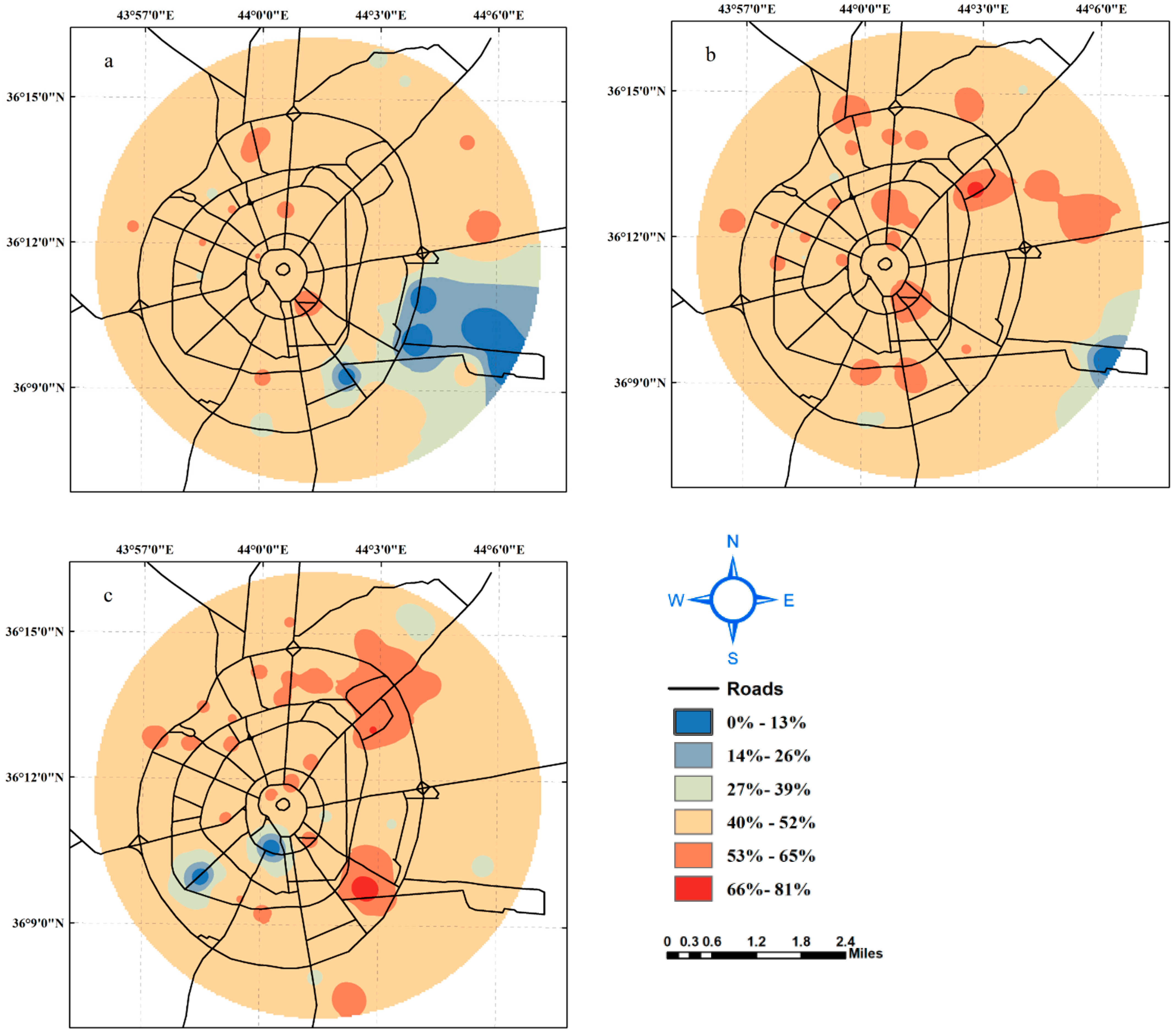
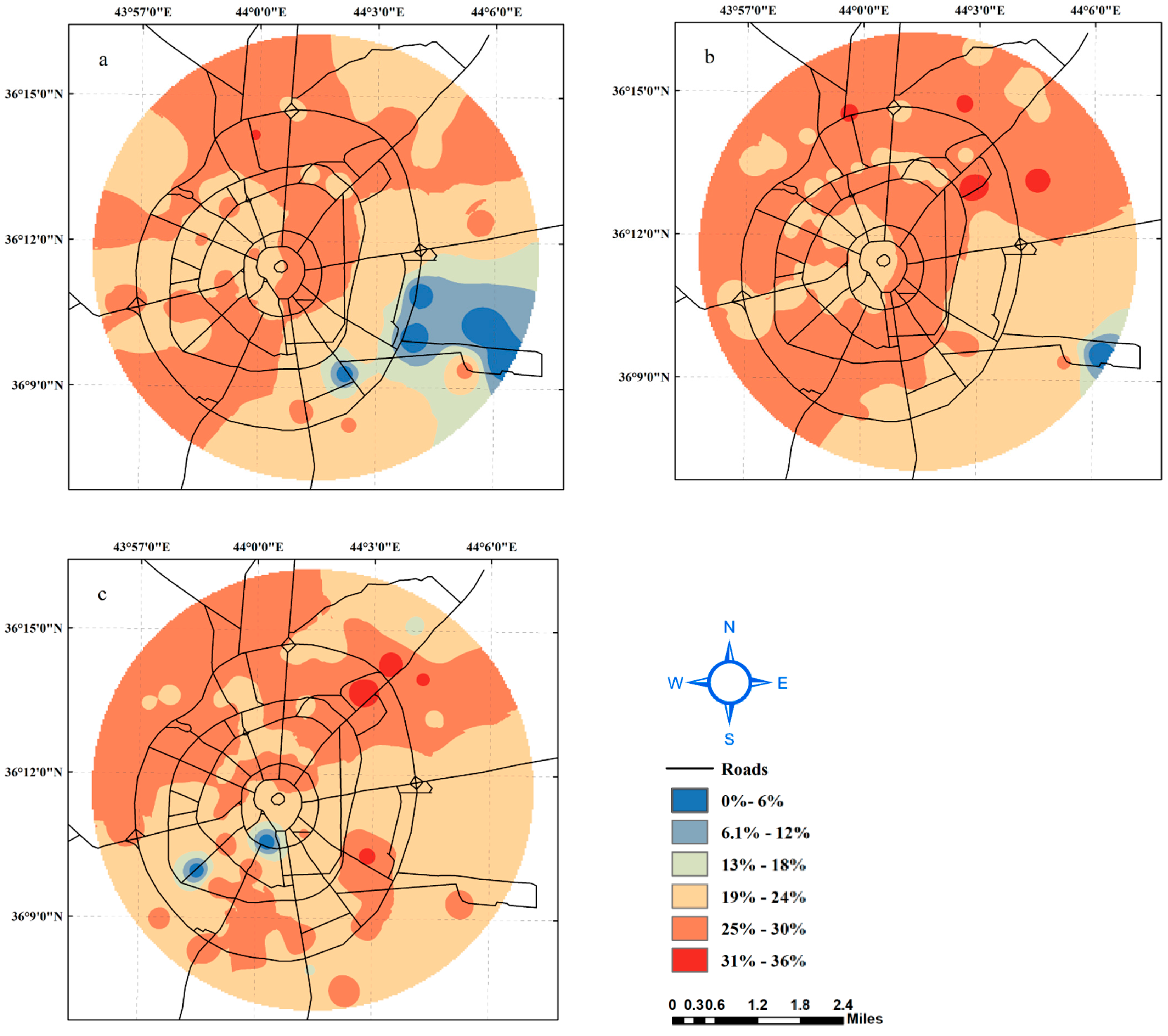
4.1.2. Atterberg Limits
4.1.3. Natural Water Content Model
4.1.4. Shear Strength Parameters
4.1.5. Consolidation Parameter Model
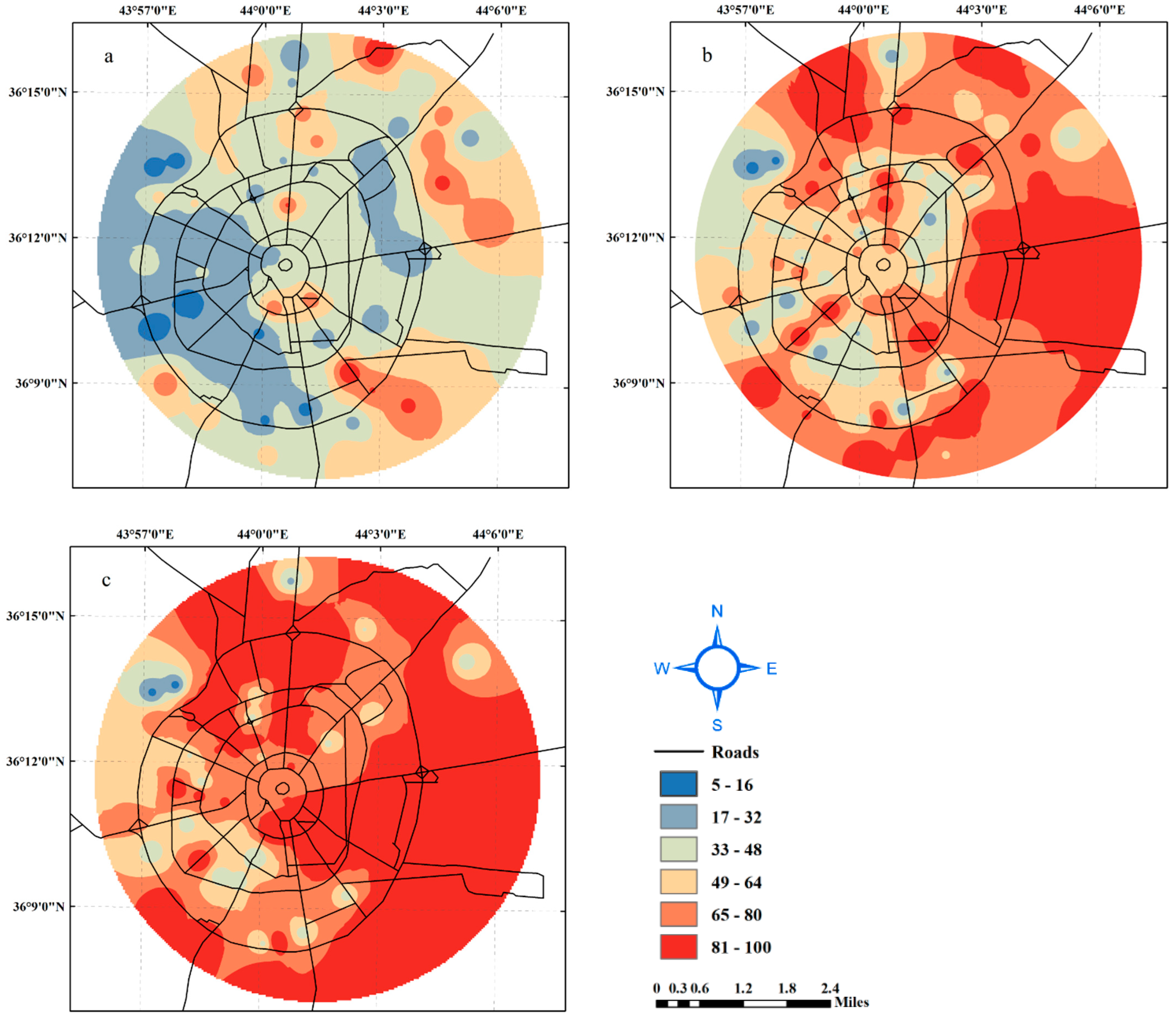
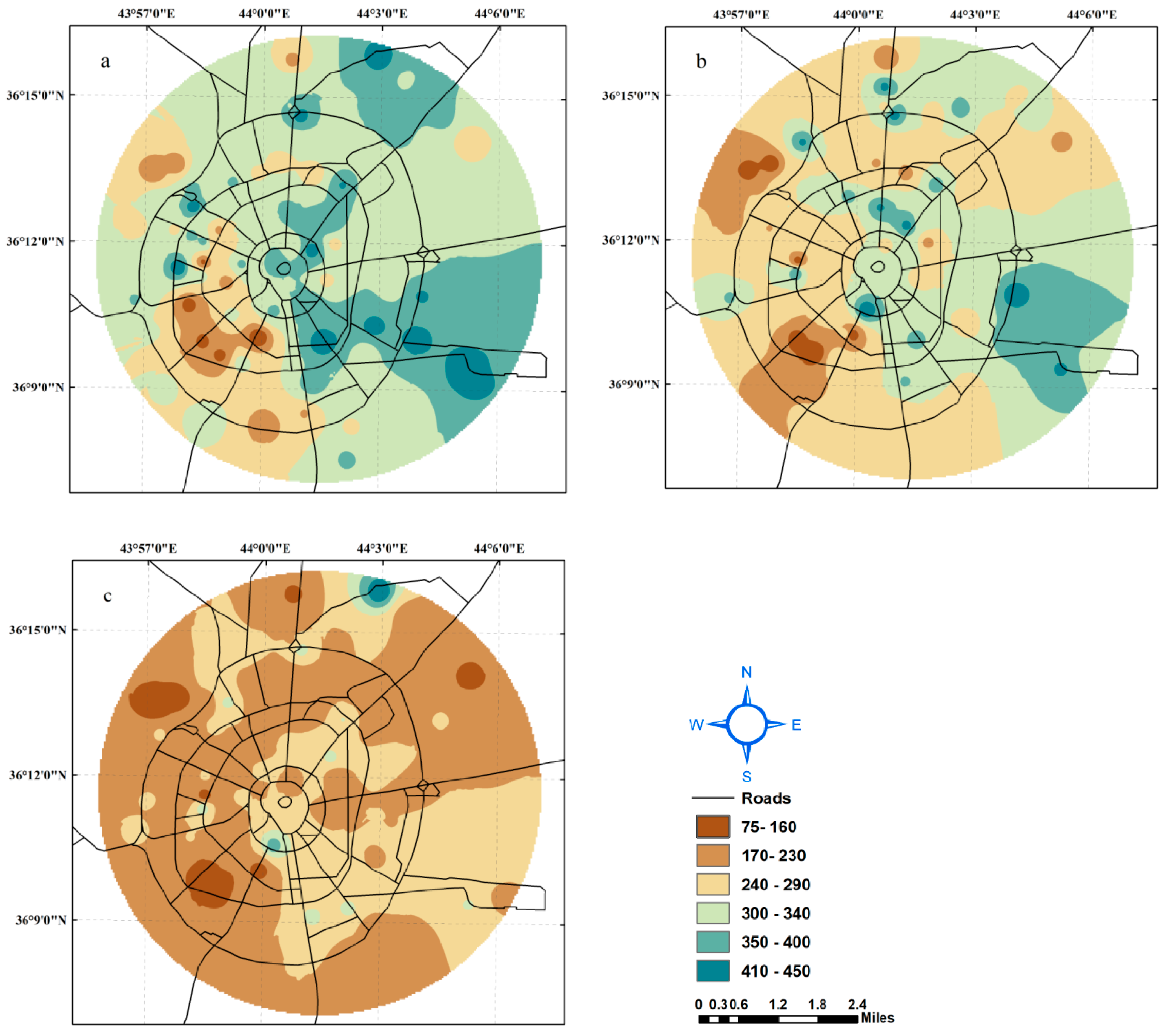
4.1.6. Standard Penetration Test Model
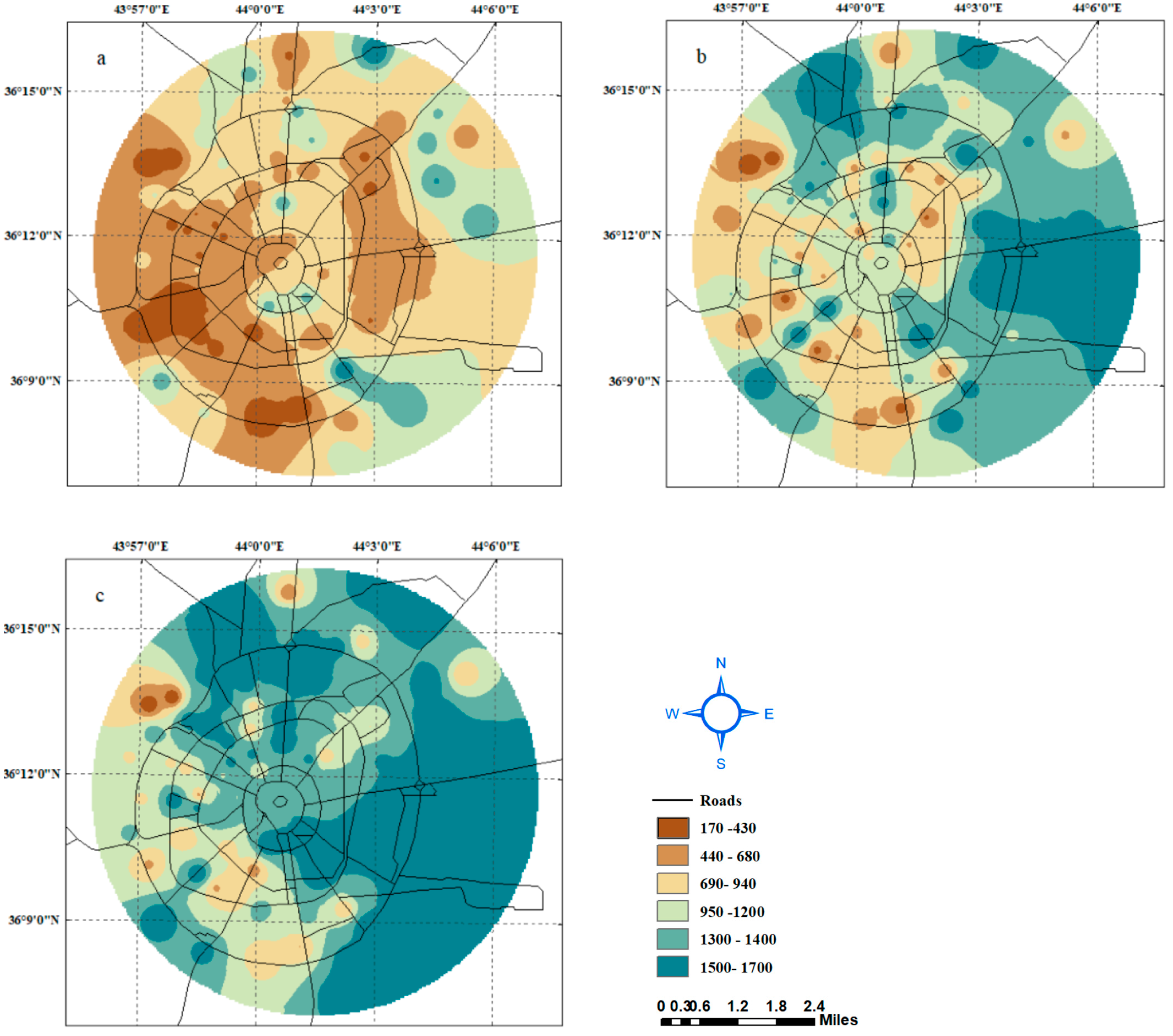
4.1.7. Bearing Capacity
4.2. Artificial Neural Network Models
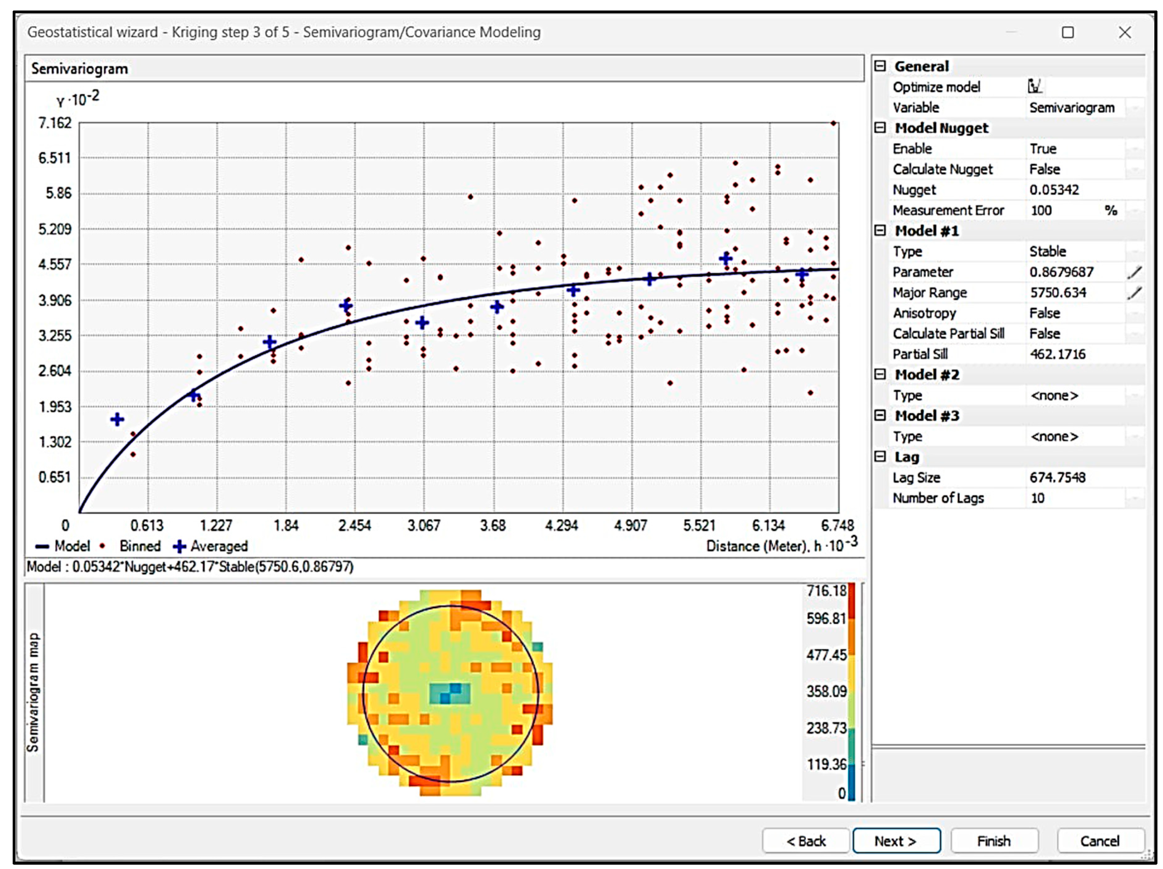
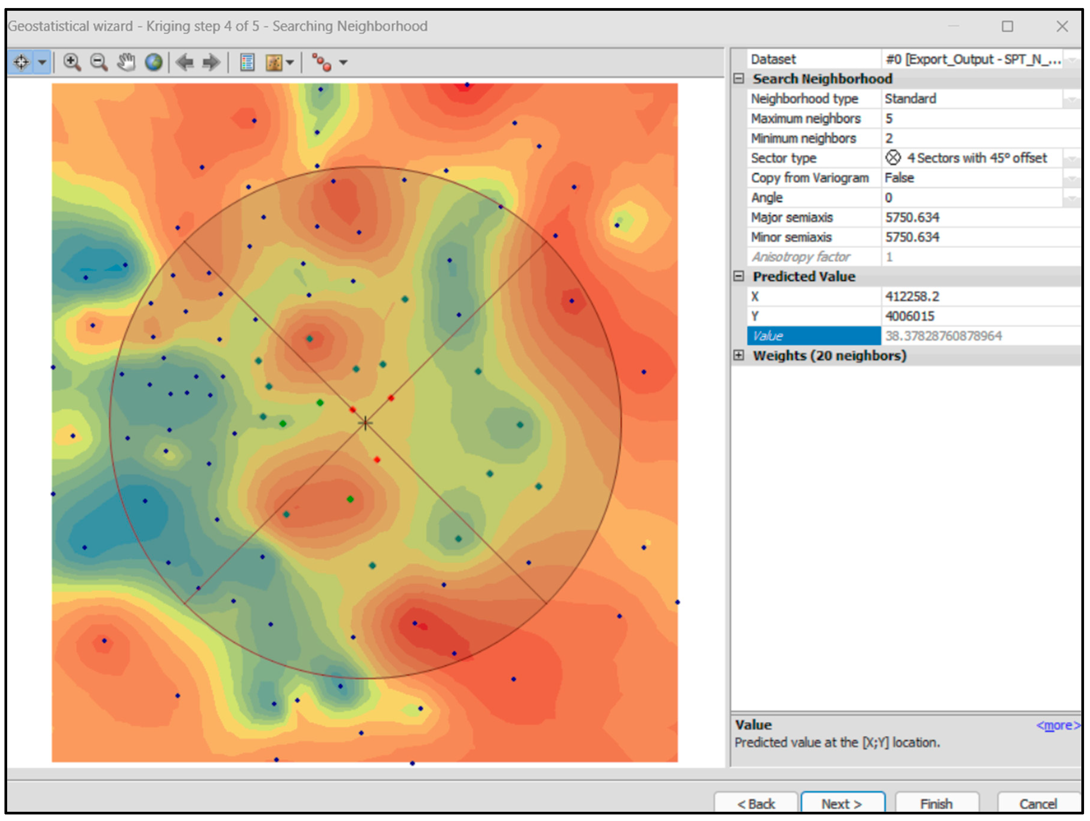
4.2.1. Validation of Interpolations Based on Semivariograms
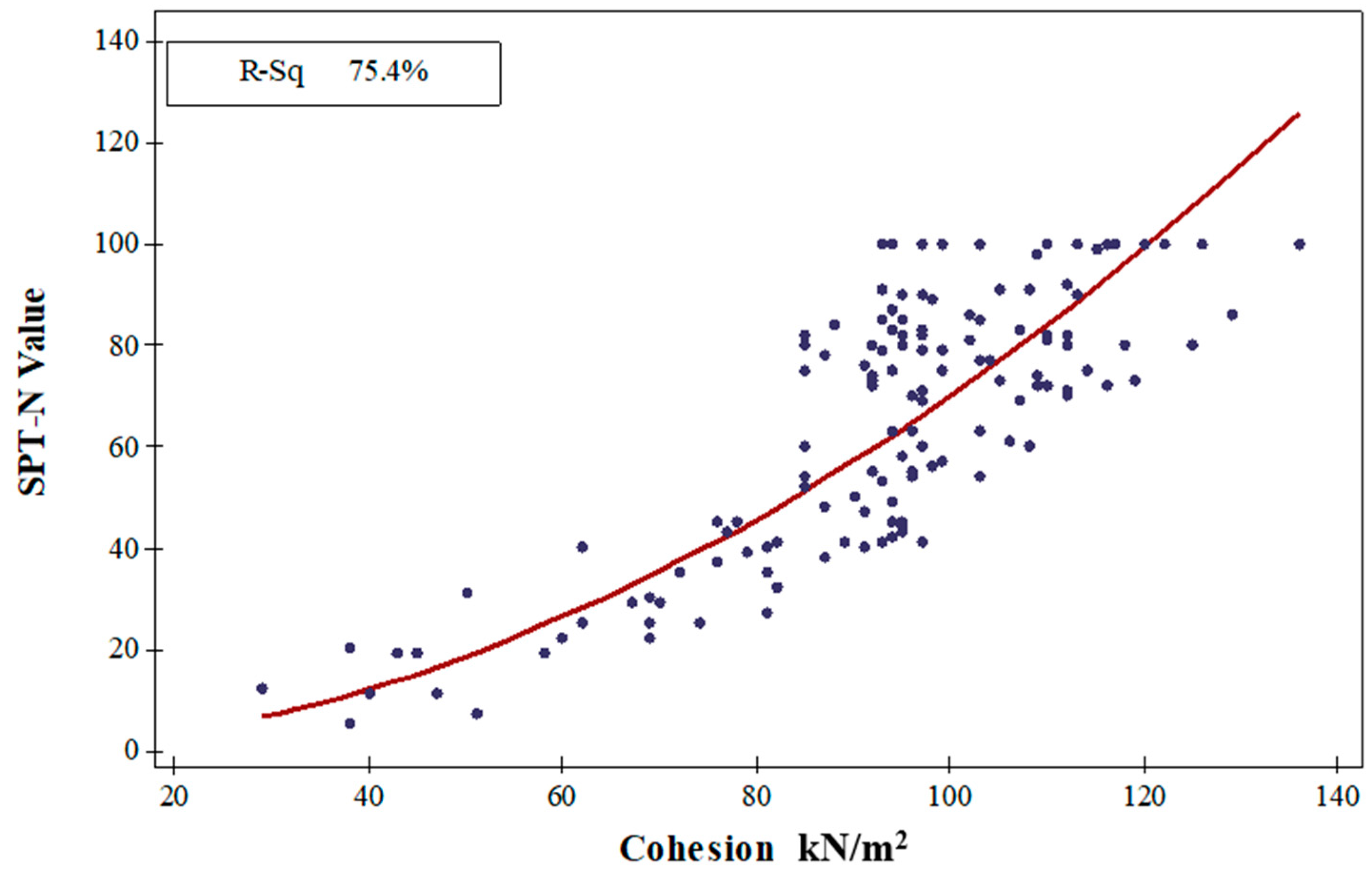
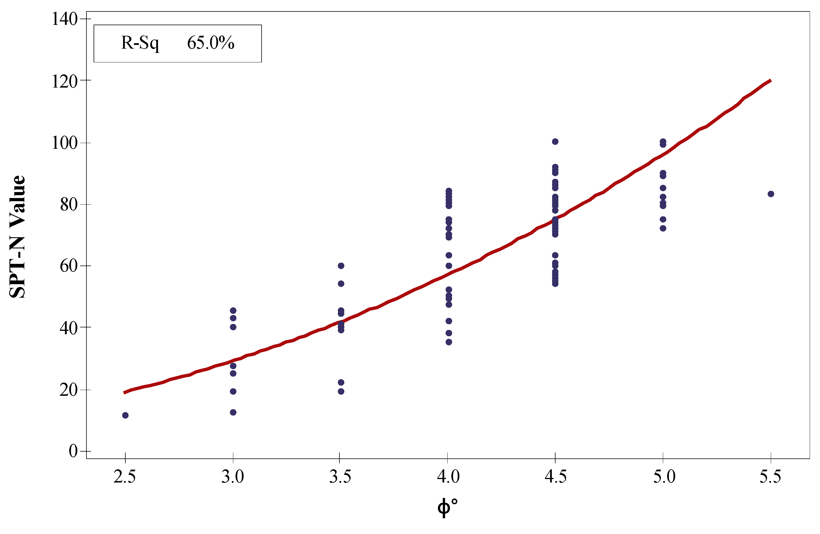
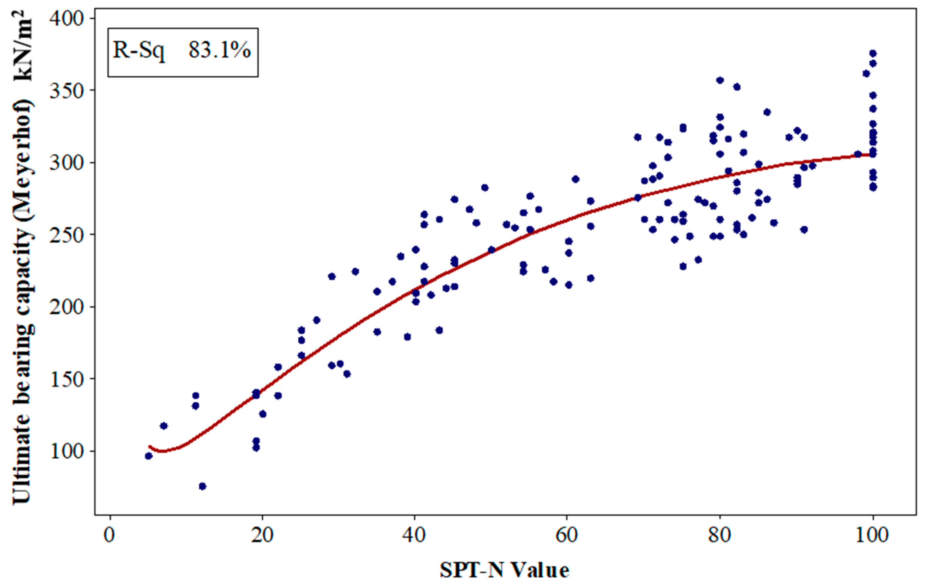
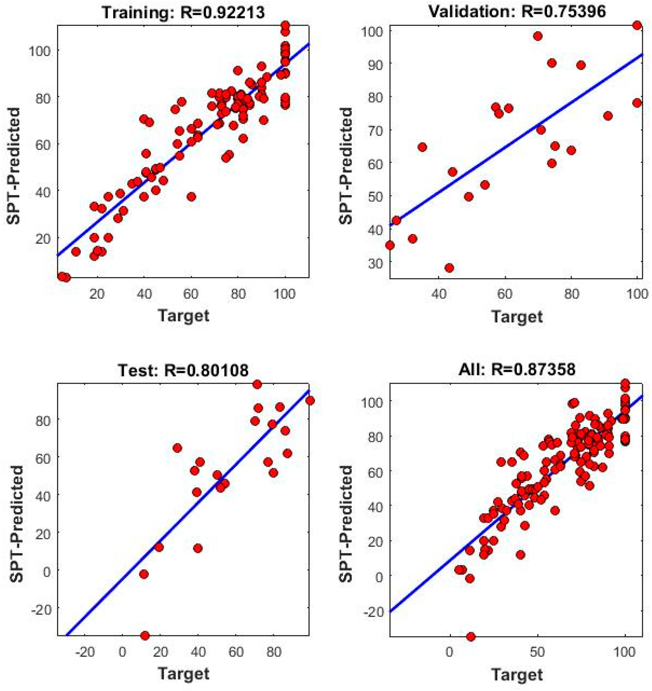
4.2.2. Prediction for SPT-N Value
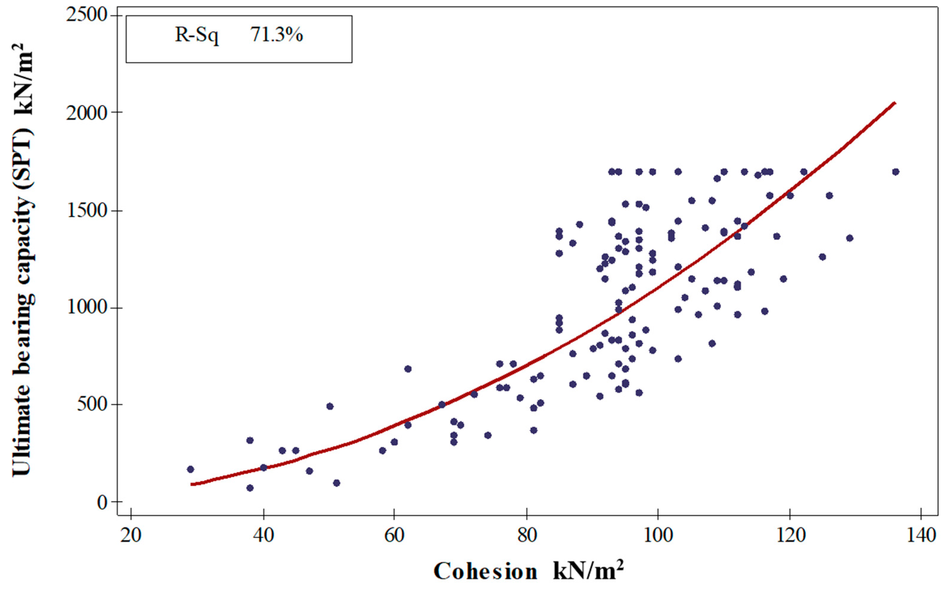
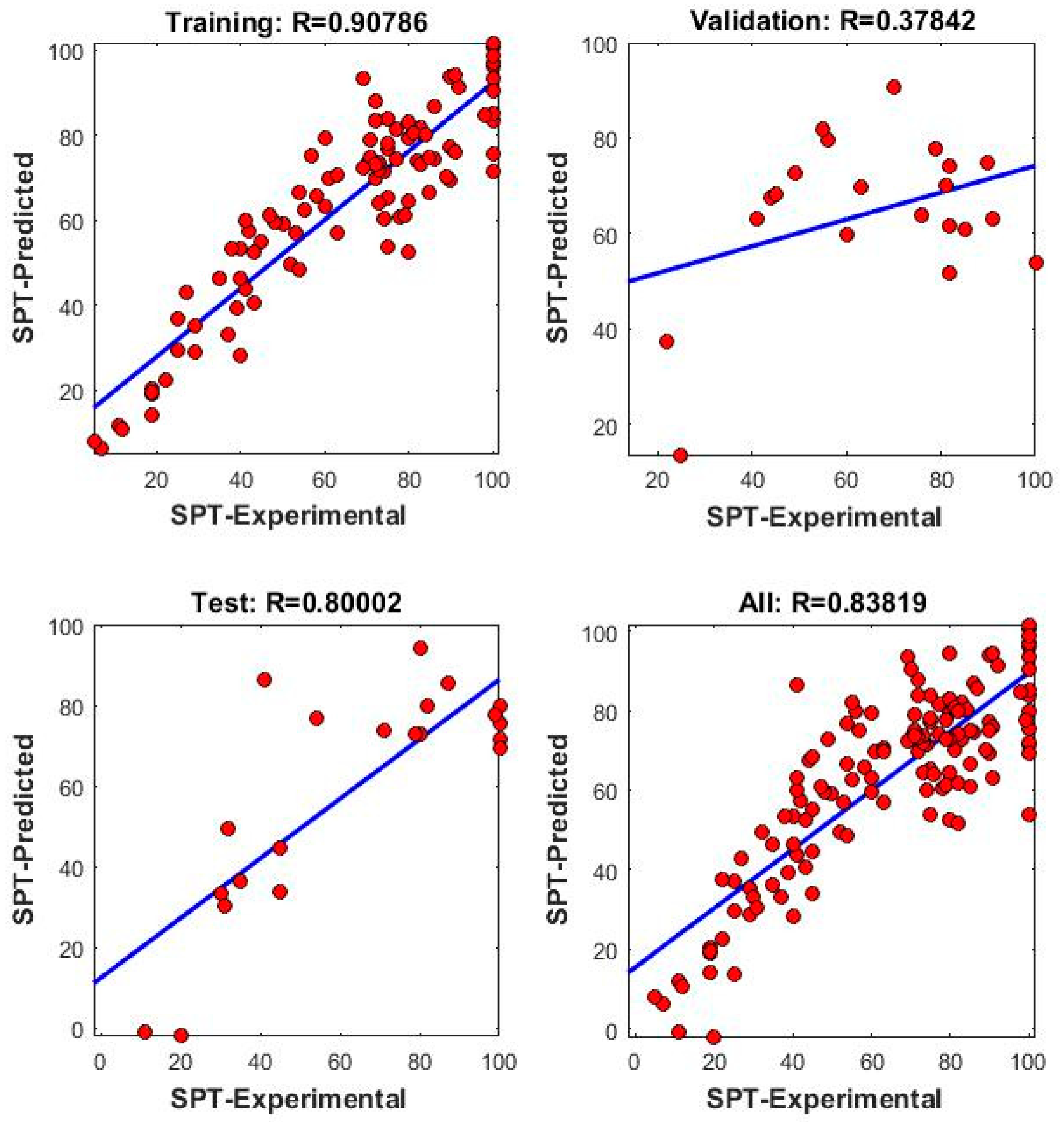
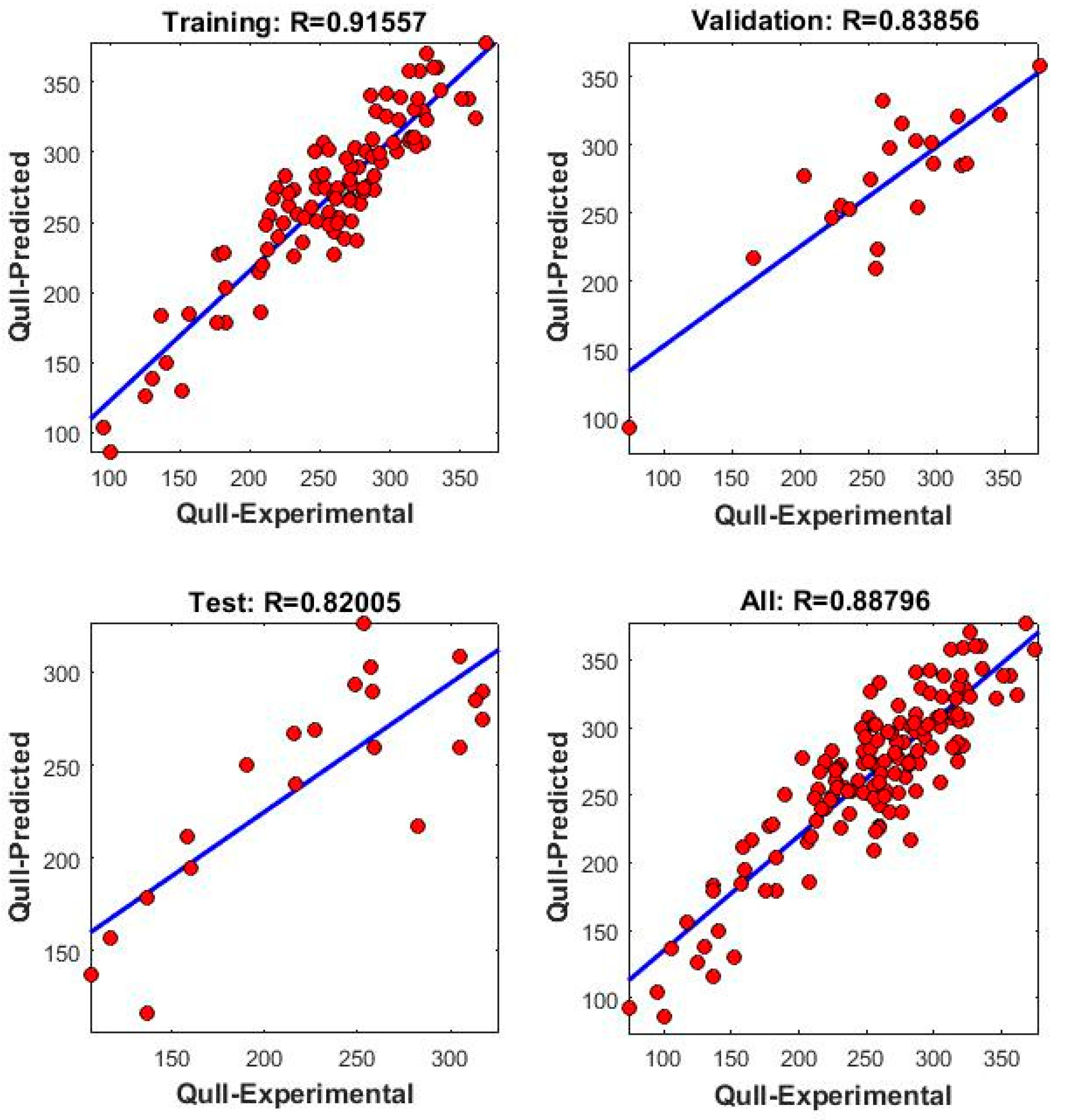
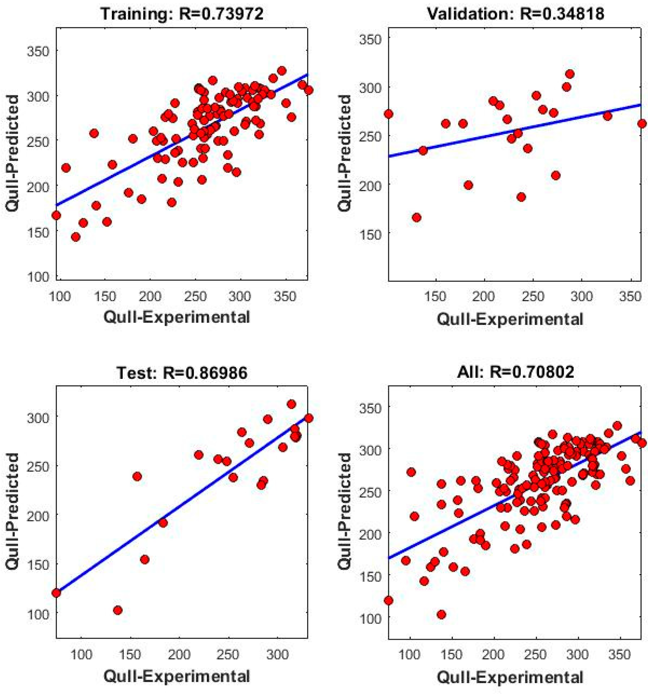
4.2.3. Prediction of Ultimate Bearing Capacity
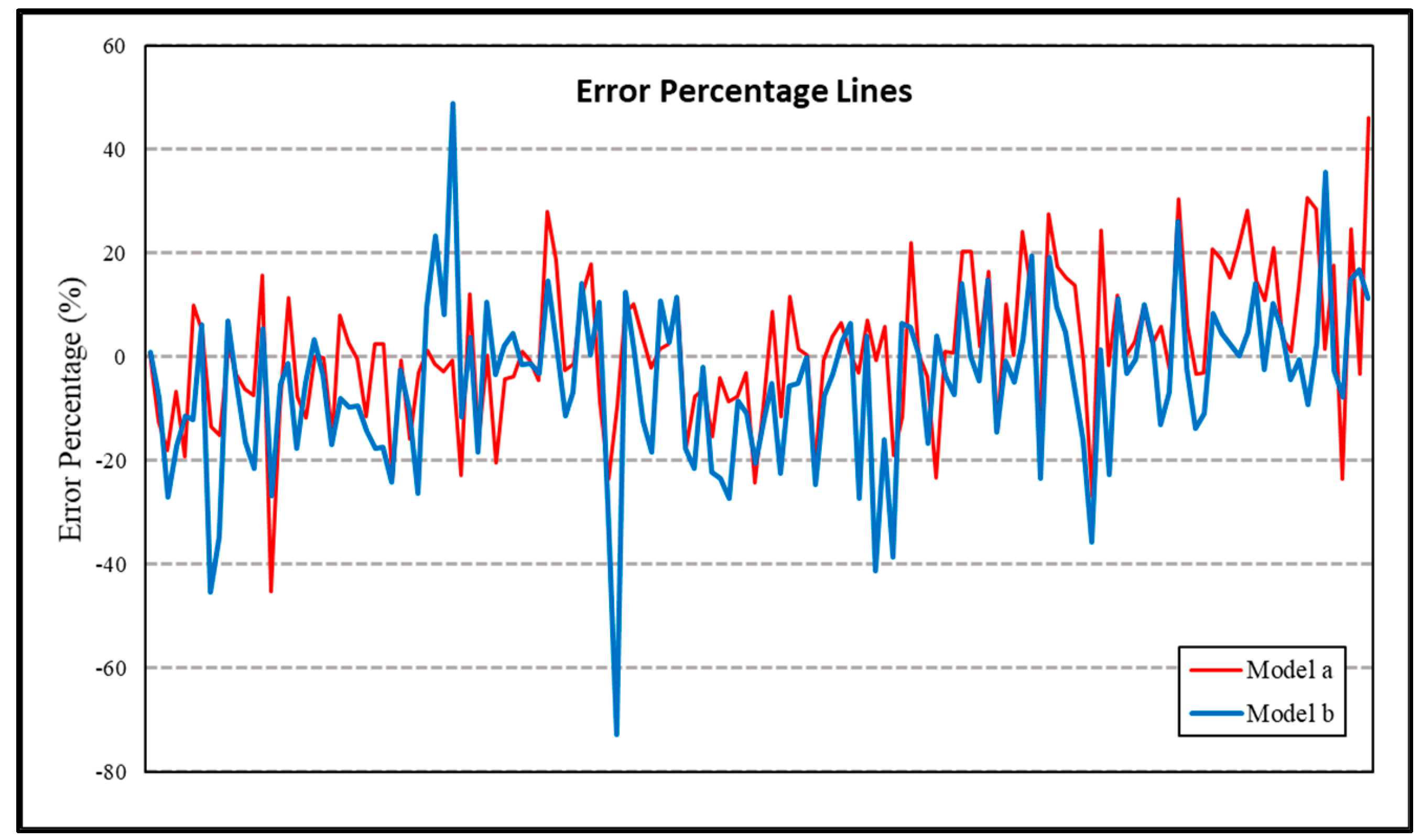
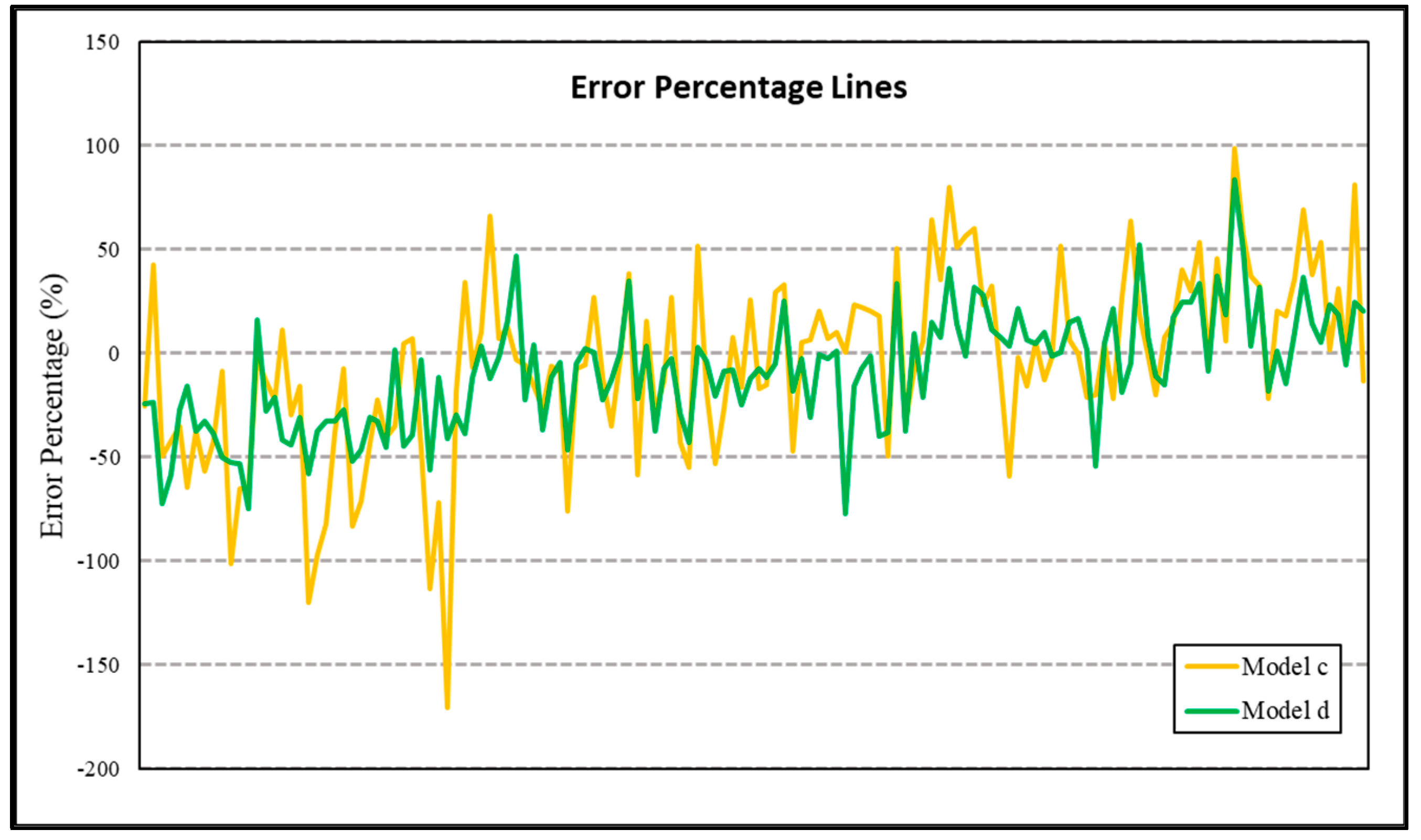
4.2.4. Percentage Error of ANN Models
4.2.5. Analysis of Models
5. Conclusions
- GIS is an effective tool that can be used by engineers to analyze the preliminary exploration of geotechnical sites. Information from 102 boreholes, considering the main geotechnical properties, was collected, evaluated, and used as input data for GIS analysis.
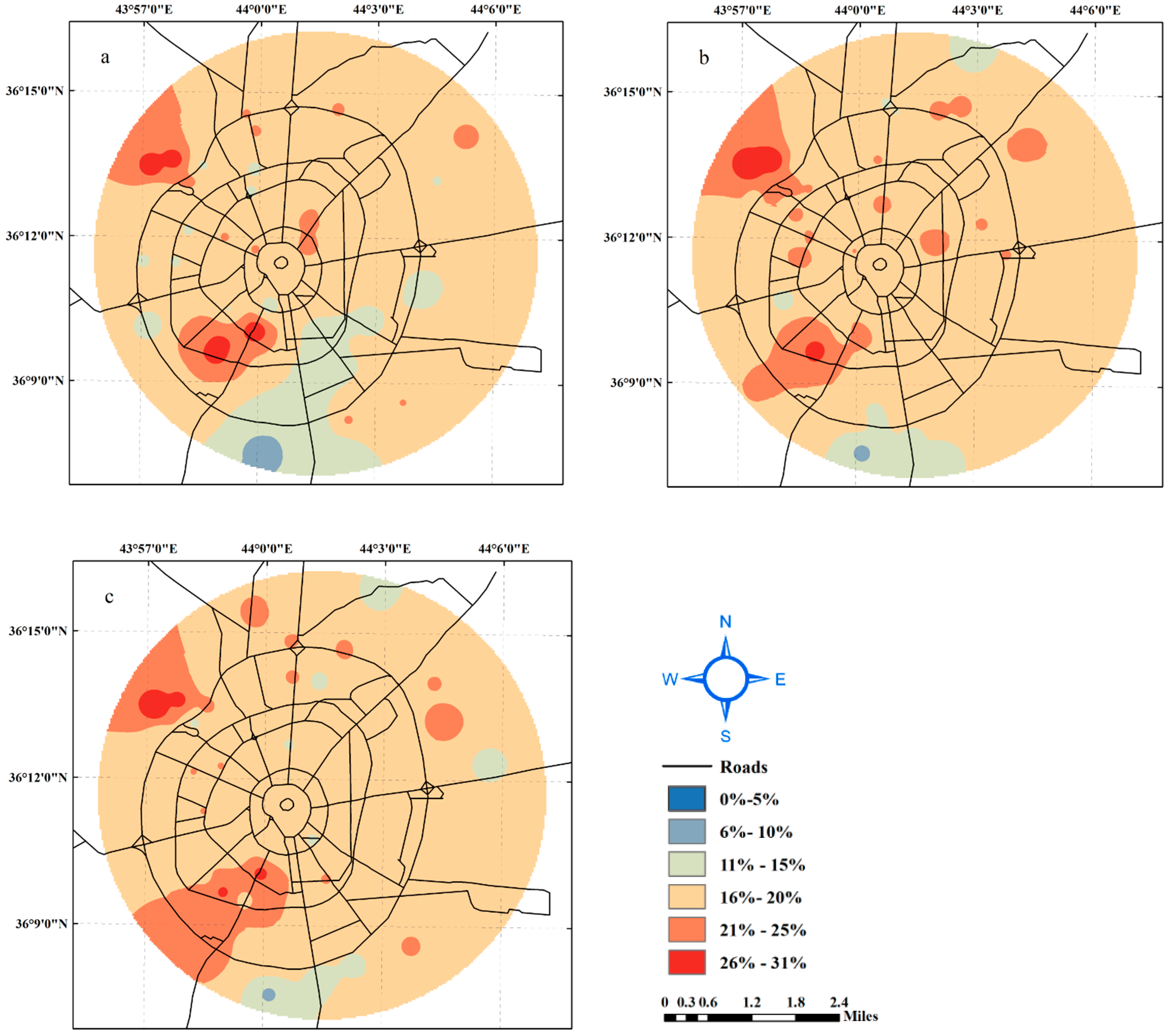
- This information suggests that a significant portion of Erbil city has soil with a high proportion of fine-grained materials, such as clay and silt. High fines content can impact the soil’s physical and engineering properties, such as its compressibility, permeability, and shear strength. The presence of high fines content can also increase the susceptibility of soil to swelling and shrinkage, which can lead to instability in structures built on or in the soil. The small zones in the southeast of the study area with lower fine contents may have different soil characteristics and may offer potential sites for structures that require more stable soil conditions. These findings are important for the design of infrastructure and buildings in the city.
- Atterberg limits in most of Erbil City were found to be between 40% and 52%, and 19% and 30% for the liquid and plastic limits, respectively. This indicates the high presence of low–plasticity clay and clayey silt. The results of the analysis of liquid limit and plastic limit values in the study area provide important information for engineers and planners in Erbil city center. They highlight the presence of low plastic clay in high percentages in the study area, as well as the need to carefully evaluate critical points with high liquid limit and plastic limit in future construction and development projects.
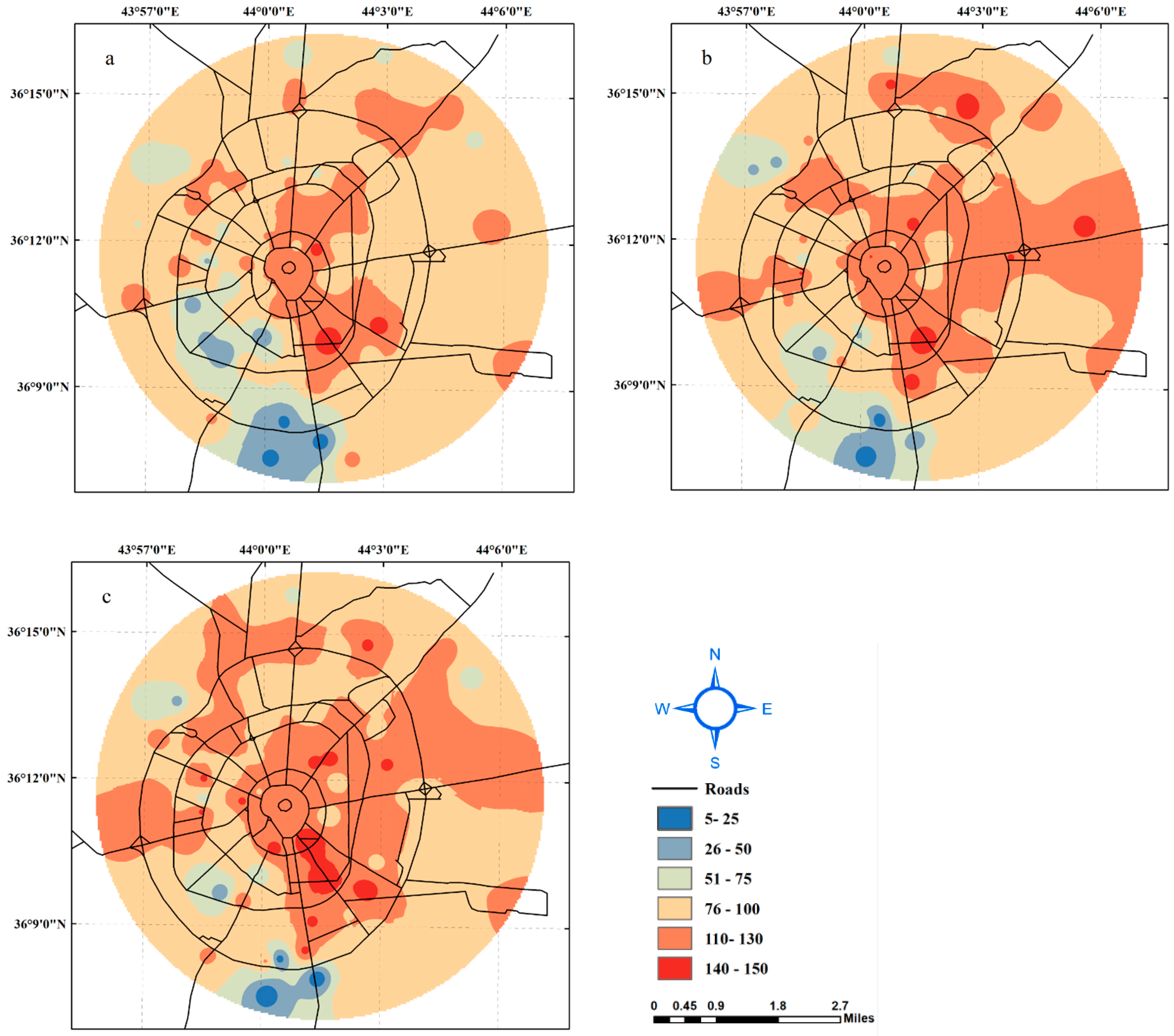
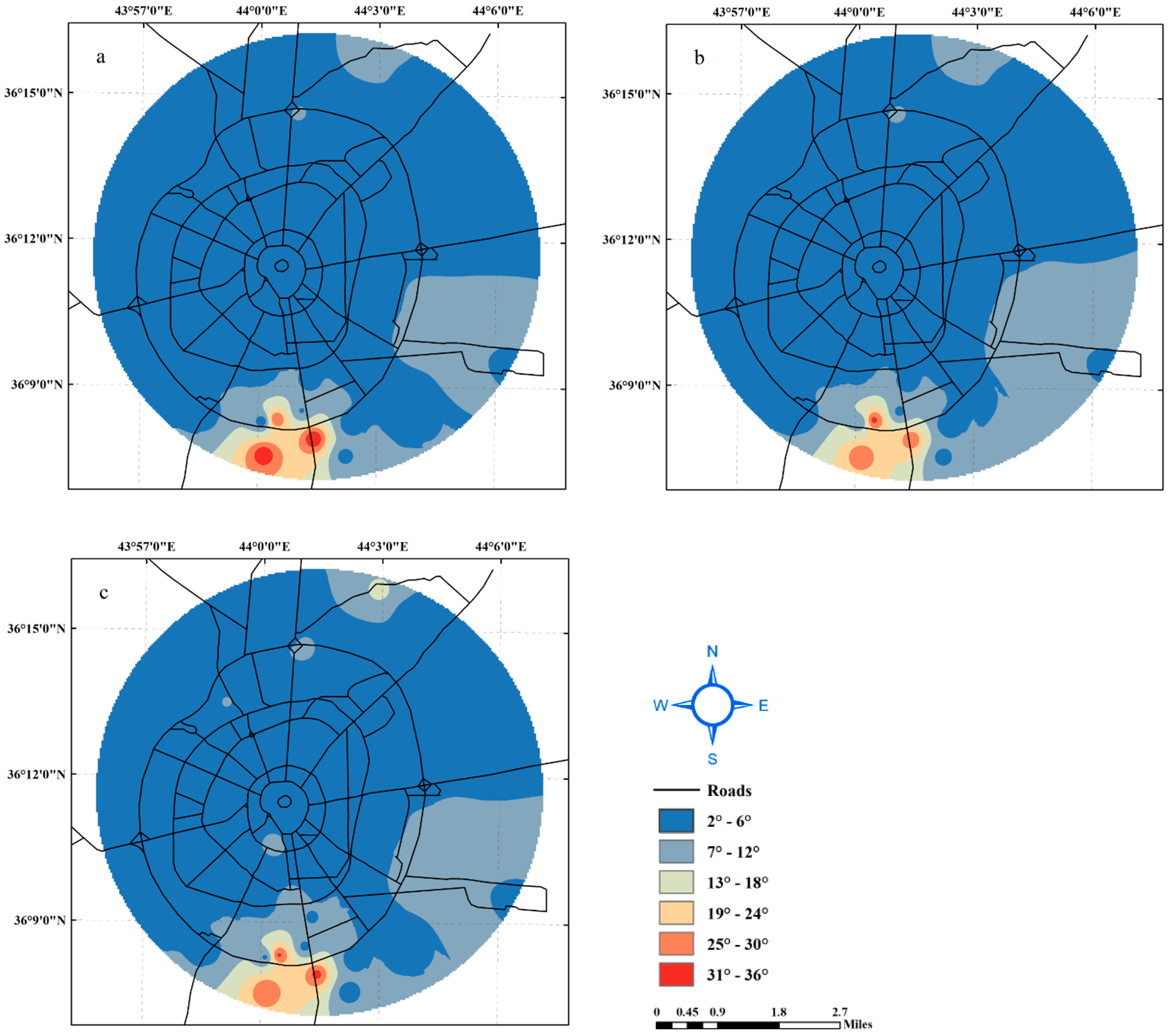
- Digital mapping of shear strength parameters showed that most soil strata at three different depths had an internal friction angle between 2° and 6°, and the cohesive strength ranged between 76 kPa and 130 kPa. The results of the cohesion values show that the soils in the study area at shallow depths have moderate to high cohesion values, and that the soils with high cohesion values tend to be located in areas with high fines content. However, the results of the angle of internal friction show that the soils in the study area have moderate to low shear strength values, with the soils in the east-south part of the area having slightly higher shear strength values. These findings are important in determining the suitability of the soil for different types of structures and in designing and constructing structures that are appropriate for the soil conditions in the area.
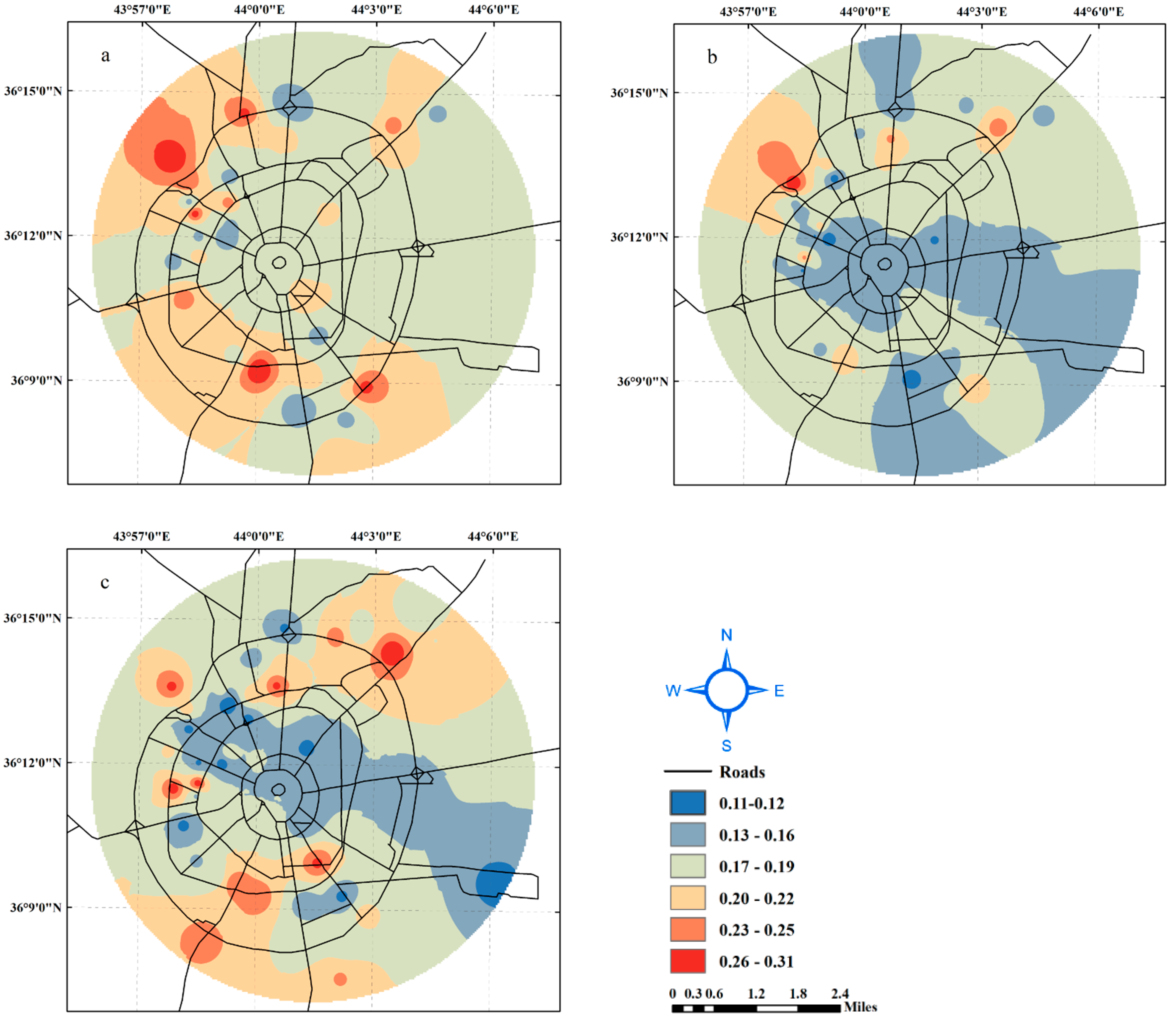
- The soil in the study area mostly has a moderate compressibility and resilience, with a moderate to low amount of rebound. The compression index decreases with depth, suggesting that the soil becomes less compressible as one moves deeper into the ground. The rebound index indicates that the soil has a moderate to low ability to recover its original volume after being compressed. These findings provide valuable information for designing structures that are built on or into the soil in the study area.
- SPT values in the study area indicate moderate soil strength in the shallow strata, with a range of 17 to 48. As the depth of the soil strata increases, the SPT values increase and become higher, covering large parts of the study area. This suggests that the soil becomes stronger with increasing depth. The SPT is a widely used in-situ test for measuring soil strength, and these results provide valuable information for the design of foundations and other structures that are supported by the soil. The higher SPT values at greater depths indicate improved soil strength characteristics and can influence the design of these structures in terms of load-bearing capacity and stability.
- This conclusion suggests that the soil in Erbil City is not capable of supporting heavy loads without modification or special design measures. The ultimate bearing capacity is a measure of the maximum weight or load that a soil can support without failure. A value lower than 170 kPa indicates that the soil may not be suitable for supporting heavy structures, such as buildings and bridges, without additional treatment or specialized foundation design. Improving the soil, such as through compaction or stabilization, and utilizing special footing designs, such piles, can increase the soil’s bearing capacity and ensure the stability and safety of structures built on the soil.
- At the preliminary design point, the completed digital geotechnical maps are vital. The designer could use the geotechnical parameters, consolidation characteristics and SPT as an effective visual display tool simply by using the digital values of these parameters for the proposed region, where the necessary decisions can be made.
- The correlation between the SPT values and shear strength parameters for the soils within the study area demonstrated a strong relationship between them.
- The results obtained from the models were compared with those measured from the field tests. It was found that predicted SPT-N values and Q-ultimate bearing capacity are quite close to the measured values. In order to check the prediction performance of the ANN model developed, several performance indices, such as R2, MAPE, and RMSE were also calculated. The ANN model has shown good prediction performance based on the performance indices. Thus, the developed ANN model can be used to predict SPT-N and Q-ultimate bearing capacity from the soil parameters and borehole coordinates. The ANN model’s implementation has also demonstrated that the neural network is a valuable tool to minimize the uncertainties encountered during geotechnical engineering projects. Therefore, using Artificial Neural Networks may provide new techniques and methodologies and minimize the potential inconsistency of correlations. ANN prediction is a useful tool for predicting the ultimate bearing capacity of soil, but it should be used in conjunction with other methods and validated with independent data to ensure accurate predictions.
Author Contributions
Funding
Institutional Review Board Statement
Informed Consent Statement
Data Availability Statement
Conflicts of Interest
Appendix A

| BH NO | DEPTH m | X | Y | LL% | PL% | PI% | WC% | c (kN/m2) | Φ (°) | Fine Content | SPT-N Value (kN/m2) |
|---|---|---|---|---|---|---|---|---|---|---|---|
| 1 | 1.5–3.5 | 406,851.5 | 4,009,570 | 46 | 22 | 24 | 28.3 | 51 | 4 | 62.1 | 7 |
| 2 | 1.5–3.5 | 405,972.9 | 4,009,284.2 | 40 | 22 | 18 | 15 | 96 | 3 | 94.1 | 54 |
| 3 | 1.5–3.5 | 407,487.6 | 4,007,947.1 | 47 | 25 | 22 | 18 | 99 | 5 | 91.5 | 57 |
| 4 | 1.5–3.5 | 406,121.1 | 4,008,204.7 | 40 | 22 | 18 | 15.0 | 96 | 3 | 94.1 | 54 |
| 5 | 1.5–3.5 | 407,443.2 | 4,008,702.7 | 50 | 27 | 23 | 20.8 | 109 | 5 | 92.9 | 41 |
| 6 | 1.5–3.5 | 407,941.4 | 4,009,347.7 | 50 | 28 | 22 | 13.9 | 108 | 4 | 91.8 | 45 |
| 7 | 1.5–3.5 | 408,217.9 | 4,008,512.23 | 35 | 20 | 19 | 20.0 | 96 | 4 | 96 | 41 |
| 8 | 1.5–3.5 | 408,997.4 | 4,008,917.8 | 39 | 21 | 18 | 16.3 | 109 | 5 | 89.4 | 45 |
| 9 | 1.5–3.5 | 408,743.4 | 4,009,398.1 | 47 | 25 | 22 | 18.0 | 99 | 5 | 91.5 | 57 |
| 10 | 1.5–3.5 | 408,026.1 | 4,010,406 | 45 | 24 | 21 | 16.6 | 96 | 5 | 95.5 | 63 |
| 11 | 1.5–3.5 | 409,617.8 | 4,011,321.6 | 46 | 27 | 19 | 20.2 | 99 | 5 | 90.7 | 41 |
| 12 | 1.5–3.5 | 408,588.1 | 4,011,780.2 | 45 | 25 | 20 | 19.0 | 97 | 4 | 91.6 | 60 |
| 13 | 1.5–3.5 | 409,762.1 | 4,012,805.4 | 48 | 26 | 22 | 19.7 | 94 | 5 | 81.3 | 75 |
| 14 | 1.5–3.5 | 411,184.2 | 4,011,787.2 | 49 | 23 | 26 | 19.6 | 108 | 4 | 96.3 | 33 |
| 15 | 1.5–3.5 | 411,184.3 | 4,012,540.7 | 47 | 25 | 22 | 15.6 | 105 | 5 | 97.4 | 30 |
| 16 | 1.5–3.5 | 411,247.7 | 4,013,522.9 | 48 | 26 | 22 | 18.4 | 58 | 3 | 92.7 | 19 |
| 17 | 1.5–3.5 | 409,969.9 | 4,010,643.8 | 58 | 31 | 27 | 20.5 | 91 | 4 | 88.9 | 40 |
| 18 | 1.5–3.5 | 409,662.9 | 4,009,977 | 56 | 30 | 26 | 18.8 | 94 | 4 | 69.1 | 42 |
| 19 | 1.5–3.5 | 409,915.1 | 4,009,232.2 | 45 | 24 | 21 | 13.6 | 77 | 3 | 95.9 | 29 |
| 20 | 1.5–3.5 | 410,862.1 | 4,009,607.35 | 44 | 25 | 19 | 18.3 | 69 | 5 | 94.5 | 30 |
| 21 | 1.5–3.5 | 411,994.6 | 4,009,216.9 | 42 | 23 | 19 | 19.2 | 70 | 4 | 98.2 | 29 |
| 22 | 1.5–3.5 | 411,166.1 | 4,010,438.9 | 50 | 26 | 24 | 17.9 | 95 | 5 | 92.2 | 58 |
| 23 | 1.5–3.5 | 412,126.9 | 4,010,308.3 | 51 | 29 | 29 | 19.8 | 95 | 5 | 96.2 | 70 |
| 24 | 1.5–3.5 | 411,550.5 | 4,011,441.2 | 44 | 23 | 21 | 14.8 | 95 | 7 | 100 | 80 |
| 25 | 1.5–3.5 | 413,143.3 | 4,011,488.9 | 44 | 25 | 19 | 20.5 | 97 | 4 | 93.5 | 41 |
| 26 | 1.5–3.5 | 414,064.7 | 4,011,692.8 | 41 | 23 | 18 | 17.4 | 110 | 4 | 53.6 | 37 |
| 27 | 1.5–3.5 | 415,317.3 | 4,010,885.4 | 50 | 26 | 24 | 15.9 | 116 | 5 | 68.5 | 23 |
| 28 | 1.5–3.5 | 414,149.3 | 4,009,671.4 | 51 | 27 | 24 | 19.1 | 94 | 4 | 87.3 | 19 |
| 29 | 1.5–3.5 | 414,362.5 | 4,008,450.6 | 52 | 24 | 28 | 19.7 | 90 | 4 | 86.4 | 17 |
| 30 | 1.5–3.5 | 416,171.1 | 4,012,249.6 | 45 | 24 | 21 | 15.3 | 98 | 6 | 79.8 | 43 |
| 31 | 1.5–3.5 | 415,609.8 | 4,012,761.8 | 38 | 21 | 17 | 16.0 | 95 | 5 | 70.6 | 45 |
| 32 | 1.5–3.5 | 414,549.1 | 4,013,637 | 38 | 21 | 17 | 70 | 12 | 97 | 100 | |
| 33 | 1.5–3.5 | 417,922.5 | 4,010,462 | 53 | 27 | 26 | 21.6 | 69 | 3 | 92.6 | 25 |
| 34 | 1.5–3.5 | 416,961.1 | 4,011,319.3 | 49 | 23 | 26 | 15.1 | 112 | 5 | 86.7 | 71 |
| 35 | 1.5–3.5 | 416,542.1 | 4,010,233.5 | 43 | 23 | 20 | 17.8 | 91 | 3 | 89.3 | 79 |
| 36 | 1.5–3.5 | 416,909.4 | 4,008,754 | 44 | 24 | 20 | 14.8 | 92 | 4 | 66.2 | 85 |
| 37 | 1.5–3.5 | 406,775.3 | 4,007,107.5 | 50 | 26 | 24 | 18.3 | 82 | 4 | 92.1 | 18 |
| 38 | 1.5–3.5 | 405,227.4 | 4,007,274.3 | 53 | 27 | 26 | 17.3 | 74 | 3 | 96.4 | 25 |
| 39 | 1.5–3.5 | 407,403.9 | 4,006,885.3 | 40 | 22 | 18 | 13.6 | 105 | 5 | 63.8 | 19 |
| 40 | 1.5–3.5 | 407,715.1 | 4,007,488.5 | 43 | 22 | 21 | 19.1 | 90 | 4 | 93.2 | 20 |
| 41 | 1.5–3.5 | 408,445.4 | 4,007,069.4 | 45 | 24 | 21 | 15.8 | 58 | 5 | 95.9 | 19 |
| 42 | 1.5–3.5 | 408,736.7 | 4,005,101.9 | 44 | 25 | 19 | 17.6 | 60 | 4 | 95.5 | 22 |
| 43 | 1.5–3.5 | 408,248.5 | 4,006,694.7 | 43 | 24 | 19 | 19.9 | 69 | 4 | 92.1 | 22 |
| 44 | 1.5–3.5 | 407,872.4 | 4,006,657.22 | 56 | 25 | 31 | 15.6 | 116 | 5 | 95.5 | 28 |
| 45 | 1.5–3.5 | 409,311.9 | 4,005,786 | 46 | 24 | 22 | 17.7 | 112 | 4 | 97.4 | 32 |
| 46 | 1.5–3.5 | 408,775.59 | 4,006,631.24 | 46 | 22 | 24 | 21.1 | 85 | 4 | 95.8 | 19 |
| 47 | 1.5–3.5 | 409,973.4 | 4,006,133 | 53 | 25 | 28 | 20.9 | 87 | 5 | 93.6 | 31 |
| 48 | 1.5–3.5 | 409,048.64 | 4,007,069.39 | 46 | 24 | 22 | 16.6 | 89 | 4 | 96.2 | 29 |
| 49 | 1.5–3.5 | 409,874.19 | 4,007,406.1 | 46 | 24 | 22 | 17.7 | 92 | 5 | 94.1 | 37 |
| 50 | 1.5–3.5 | 408,985.14 | 4,007,907.6 | 54 | 26 | 28 | 15.3 | 99 | 4 | 94.1 | 39 |
| 51 | 1.5–3.5 | 411,015.2 | 4,007,902.7 | 55 | 24 | 31 | 15.3 | 112 | 5 | 95.2 | 82 |
| 52 | 1.5–3.5 | 418,521.8 | 4,007,163.4 | 57 | 25 | 32 | 19.6 | 104 | 4 | 92.9 | 77 |
| 53 | 1.5–3.5 | 409,785.25 | 4,008,333.1 | 48 | 22 | 26 | 14.4 | 97 | 4 | 95.5 | 22 |
| 54 | 1.5–3.5 | 410,998.6 | 4,008,878.3 | 49 | 26 | 23 | 18.8 | 105 | 4 | 92.2 | 32 |
| 55 | 1.5–3.5 | 410,109.1 | 4,006,834.44 | 41 | 19 | 22 | 16.8 | 101 | 4 | 87.3 | 41 |
| 56 | 1.5–3.5 | 410,419.8 | 4,006,001 | 45 | 21 | 24 | 16.3 | 123 | 5 | 52.3 | 28 |
| 57 | 1.5–3.5 | 412,049.02 | 4,007,215.97 | 52 | 24 | 28 | 21.8 | 109 | 5 | 51.8 | 44 |
| 58 | 1.5–3.5 | 411,263 | 4,006,447.5 | 51 | 27 | 24 | 19.4 | 96 | 4 | 94.2 | 33 |
| 59 | 1.5–3.5 | 412,664.18 | 4,007,328.4 | 49 | 25 | 24 | 19.4 | 124 | 4 | 92.6 | 38 |
| 60 | 1.5–3.5 | 411,990 | 4,006,315.2 | 44 | 25 | 19 | 21.7 | 136 | 5 | 95.7 | 39 |
| 61 | 1.5–3.5 | 413,164.9 | 4,008,779 | 43 | 23 | 20 | 18.9 | 119 | 5 | 96.6 | 41 |
| 62 | 1.5–3.5 | 412,846.74 | 4,006,559.81 | 49 | 26 | 23 | 17.4 | 79 | 4 | 93.5 | 39 |
| 63 | 1.5–3.5 | 412,536.5 | 4,005,174.2 | 48 | 27 | 21 | 18.0 | 81 | 4 | 93.5 | 35 |
| 64 | 1.5–3.5 | 415,747.4 | 4,005,960.69 | 48 | 23 | 25 | 16.8 | 96 | 4 | 96.4 | 21 |
| 65 | 1.5–3.5 | 414,814.8 | 4,007,156.9 | 40 | 21 | 19 | 17.9 | 97 | 5 | 39.7 | 31 |
| 66 | 1.5–3.5 | 415,071.9 | 4,004,866.9 | 47 | 24 | 23 | 19.0 | 95 | 5 | 90.8 | 34 |
| 67 | 1.5–3.5 | 417,971.23 | 4,001,685.01 | 48 | 27 | 21 | 17.4 | 88 | 8 | 30 | 61 |
| 68 | 1.5–3.5 | 418,519 | 4,003,222.9 | 0 | 0 | 0 | 17.7 | 85 | 10 | 18 | 37 |
| 69 | 1.5–3.5 | 415,926 | 4,002,878 | 0 | 0 | 0 | 19.0 | 83 | 9 | 14 | 50 |
| 70 | 1.5–3.5 | 416,167 | 4,004,572.3 | 0 | 0 | 0 | 11.0 | 80 | 8 | 15 | 36 |
| 71 | 1.5–3.5 | 419,289 | 4,001,977.6 | 0 | 0 | 0 | 18.6 | 114 | 5 | 25 | 40 |
| 72 | 1.5–3.5 | 411,924.27 | 4,004,297.59 | 57 | 25 | 32 | 16.4 | 116 | 5 | 94.7 | 72 |
| 73 | 1.5–3.5 | 410,482.29 | 4,003,953.63 | 48 | 23 | 25 | 13.4 | 109 | 5 | 91.4 | 74 |
| 74 | 1.5–3.5 | 412,426.98 | 4,002,802.69 | 45 | 21 | 24 | 12.1 | 144 | 4 | 95.6 | 23 |
| 75 | 1.5–3.5 | 414,365 | 4,003,408 | 44 | 21 | 23 | 13.7 | 135 | 4 | 94.6 | 20 |
| 76 | 1.5–3.5 | 411,975.73 | 4,001,202.95 | 47 | 21 | 26 | 13.8 | 118 | 5 | 93.2 | 39 |
| 77 | 1.5–3.5 | 414,022.9 | 4,002,387 | 45 | 22 | 23 | 15.4 | 95 | 4 | 94.7 | 44 |
| 78 | 1.5–3.5 | 411,697.91 | 4,000,107.57 | 41 | 27 | 14 | 11.9 | 55 | 6 | 77.8 | 8 |
| 79 | 1.5–3.5 | 410,200 | 3,999,706 | 35 | 23 | 12 | 12.6 | 47 | 3 | 83.7 | 11 |
| 80 | 1.5–3.5 | 413,372.73 | 4,001,528.38 | 0 | 0 | 0 | 13.7 | 98 | 5 | 8.4 | 100 |
| 81 | 1.5–3.5 | 414,253.79 | 4,000,845.76 | 47 | 22 | 25 | 17.5 | 86 | 5 | 91.7 | 81 |
| 82 | 1.5–3.5 | 415,598.5 | 4,000,259 | 45 | 22 | 24 | 20.1 | 89 | 3 | 93.5 | 83 |
| 83 | 1.5–3.5 | 413,510.13 | 3,999,595.57 | 47 | 25 | 22 | 20.5 | 81 | 3 | 95.6 | 27 |
| 84 | 1.5–3.5 | 412,160.93 | 3,999,051.88 | 41 | 22 | 19 | 12.7 | 12 | 36 | 100 | 45 |
| 85 | 1.5–3.5 | 410,732.9 | 3,999,785 | 40 | 21 | 19 | 10.8 | 15 | 30 | 33 | 47 |
| 86 | 1.5–3.5 | 410,253 | 3,998,445 | 43 | 23 | 20 | 5.7 | 19 | 35 | 42 | 53 |
| 87 | 1.5–3.5 | 413,309 | 3,998,392.5 | 41 | 21 | 20 | 12.3 | 108 | 5 | 81.6 | 60 |
| 88 | 1.5–3.5 | 410,136.16 | 4,001,490.72 | 55 | 26 | 29 | 17.3 | 81 | 3 | 96.2 | 22 |
| 89 | 1.5–3.5 | 409,296.11 | 4,002,026.51 | 46 | 24 | 22 | 22.1 | 96 | 5 | 96.8 | 31 |
| 90 | 1.5–3.5 | 408,932.6 | 4,003,851.9 | 50 | 24 | 26 | 14.8 | 90 | 3 | 97.3 | 29 |
| 91 | 1.5–3.5 | 408,515.58 | 4,002,310.93 | 44 | 30 | 14 | 31.1 | 25 | 2 | 90.1 | 18 |
| 92 | 1.5–3.5 | 409,939 | 4,003,009.6 | 44 | 28 | 16 | 29.2 | 29 | 3 | 89.2 | 12 |
| 93 | 1.5–3.5 | 407,821.05 | 4,002,866.56 | 42 | 21 | 21 | 23.2 | 45 | 4 | 91.6 | 19 |
| 94 | 1.5–3.5 | 407,298.5 | 4,004,255.62 | 49 | 26 | 23 | 16.7 | 38 | 3 | 89.8 | 5 |
| 95 | 1.5–3.5 | 405,937 | 4,003,224 | 43 | 23 | 20 | 13.3 | 90 | 4 | 93.3 | 7 |
| 96 | 1.5–3.5 | 407,774.75 | 4,005,380.1 | 38 | 21 | 17 | 16.9 | 98 | 4 | 96.6 | 39 |
| 97 | 1.5–3.5 | 407,844.33 | 4,005,870.11 | 39 | 22 | 17 | 18.9 | 43 | 4 | 56.7 | 19 |
| 98 | 1.5–3.5 | 406,914.85 | 4,005,671.15 | 45 | 23 | 22 | 14.5 | 121 | 6 | 94.6 | 23 |
| 99 | 1.5–3.5 | 405,242 | 4,004,431.7 | 46 | 25 | 21 | 15.6 | 110 | 4 | 98.1 | 25 |
| 100 | 1.5–3.5 | 405,684.54 | 4,005,717.45 | 43 | 21 | 22 | 14.8 | 95 | 4 | 94.3 | 41 |
| 101 | 1.5–3.5 | 408,025.12 | 3,999,907.5 | 46 | 24 | 22 | 15.7 | 103 | 4 | 96.2 | 54 |
| 102 | 1.5–3.5 | 406,400.4 | 4,001,124 | 42 | 26 | 16 | 15.5 | 94 | 4 | 96.1 | 75 |
| 103 | 3.5–6.5 | 406,851.5 | 4,009,570 | 49 | 23 | 26 | 29.4 | 40 | 4 | 83.5 | 11 |
| 104 | 3.5–6.5 | 405,972.9 | 4,009,284.2 | 48 | 23 | 25 | 29.1 | 45 | 5 | 87 | 9 |
| 105 | 3.5–6.5 | 407,487.6 | 4,007,947.1 | 50 | 24 | 26 | 19.2 | 109 | 5 | 95.1 | 72 |
| 106 | 3.5–6.5 | 406,121.1 | 4,008,204.7 | 46 | 26 | 20 | 19.4 | 85 | 4 | 97.9 | 60 |
| 107 | 3.5–6.5 | 407,443.2 | 4,008,702.7 | 52 | 26 | 26 | 23.2 | 112 | 4 | 94.9 | 70 |
| 108 | 3.5–6.5 | 407,941.4 | 4,009,347.7 | 52 | 29 | 23 | 14.8 | 103 | 4 | 93.7 | 77 |
| 109 | 3.5–6.5 | 408,217.9 | 4,008,512.23 | 40 | 22 | 18 | 20.5 | 113 | 5 | 100 | 90 |
| 110 | 3.5–6.5 | 408,997.4 | 4,008,917.8 | 36 | 23 | 13 | 105 | 5 | 98.4 | 73 | |
| 111 | 3.5–6.5 | 408,743.4 | 4,009,398.1 | 44 | 24 | 20 | 19.3 | 102 | 5 | 95.1 | 86 |
| 112 | 3.5–6.5 | 408,026.1 | 4,010,406 | 42 | 23 | 19 | 15.5 | 102 | 6 | 94.1 | 80 |
| 113 | 3.5–6.5 | 409,617.8 | 4,011,321.6 | 64 | 33 | 31 | 19.5 | 89 | 4 | 80.5 | 97 |
| 114 | 3.5–6.5 | 408,588.1 | 4,011,780.2 | 48 | 25 | 23 | 20.1 | 93 | 5 | 89.1 | 99 |
| 115 | 3.5–6.5 | 409,762.1 | 4,012,805.4 | 46 | 25 | 21 | 17.2 | 98 | 5 | 72.5 | 100 |
| 116 | 3.5–6.5 | 411,184.2 | 4,011,787.2 | 45 | 24 | 21 | 14.3 | 104 | 4 | 95.7 | 50 |
| 117 | 3.5–6.5 | 411,184.3 | 4,012,540.7 | 49 | 28 | 21 | 18.2 | 132 | 6 | 92.9 | 62 |
| 118 | 3.5–6.5 | 411,247.7 | 4,013,522.9 | 45 | 27 | 18 | 19.0 | 62 | 4 | 100 | 25 |
| 119 | 3.5–6.5 | 409,969.9 | 4,010,643.8 | 51 | 27 | 24 | 18.7 | 93 | 5 | 94.3 | 91 |
| 120 | 3.5–6.5 | 409,662.9 | 4,009,977 | 54 | 29 | 25 | 19.3 | 95 | 5 | 94.2 | 89 |
| 121 | 3.5–6.5 | 409,915.1 | 4,009,232.2 | 47 | 23 | 24 | 17.5 | 87 | 5 | 94.6 | 33 |
| 122 | 3.5–6.5 | 410,862.1 | 4,009,607.35 | 46 | 22 | 24 | 20.7 | 82 | 4 | 98.2 | 41 |
| 123 | 3.5–6.5 | 411,994.6 | 4,009,216.9 | 45 | 21 | 23 | 17.0 | 72 | 5 | 97.5 | 35 |
| 124 | 3.5–6.5 | 411,166.1 | 4,010,438.9 | 54 | 25 | 29 | 18.6 | 91 | 4 | 97.8 | 76 |
| 125 | 3.5–6.5 | 412,126.9 | 4,010,308.3 | 55 | 26 | 29 | 19.3 | 93 | 4 | 92.1 | 79 |
| 126 | 3.5–6.5 | 411,550.5 | 4,011,441.2 | 46 | 22 | 24 | 14.8 | 97 | 8 | 100 | 100 |
| 127 | 3.5–6.5 | 413,143.3 | 4,011,488.9 | 46 | 25 | 21 | 21.1 | 99 | 4 | 95.2 | 75 |
| 128 | 3.5–6.5 | 414,064.7 | 4,011,692.8 | 60 | 32 | 28 | 21.2 | 147 | 5 | 86.6 | 50 |
| 129 | 3.5–6.5 | 415,317.3 | 4,010,885.4 | 50 | 28 | 22 | 20.2 | 98 | 5 | 91.9 | 56 |
| 130 | 3.5–6.5 | 414,149.3 | 4,009,671.4 | 42 | 23 | 19 | 19.4 | 95 | 5 | 41.6 | 100 |
| 131 | 3.5–6.5 | 414,362.5 | 4,008,450.6 | 71 | 36 | 35 | 19.7 | 95 | 5 | 59.7 | 43 |
| 132 | 3.5–6.5 | 416,171.1 | 4,012,249.6 | 38 | 21 | 17 | 16.8 | 95 | 5 | 82.6 | 82 |
| 133 | 3.5–6.5 | 415,609.8 | 4,012,761.8 | 44 | 25 | 19 | 16.1 | 97 | 6 | 85.8 | 83 |
| 134 | 3.5–6.5 | 414,549.1 | 4,013,637 | 42 | 23 | 19 | 10.4 | 75 | 11 | 100 | 100 |
| 135 | 3.5–6.5 | 417,922.5 | 4,010,462 | 48 | 26 | 22 | 20.2 | 76 | 5 | 96.1 | 37 |
| 136 | 3.5–6.5 | 416,961.1 | 4,011,319.3 | 48 | 23 | 25 | 114 | 5 | 69.1 | 75 | |
| 137 | 3.5–6.5 | 416,542.1 | 4,010,233.5 | 45 | 26 | 19 | 21.6 | 94 | 5 | 94.9 | 87 |
| 138 | 3.5–6.5 | 416,909.4 | 4,008,754 | 54 | 32 | 22 | 19.6 | 94 | 4 | 89.4 | 83 |
| 139 | 3.5–6.5 | 406,775.3 | 4,007,107.5 | 53 | 28 | 25 | 19.3 | 78 | 3 | 97.9 | 45 |
| 140 | 3.5–6.5 | 405,227.4 | 4,007,274.3 | 54 | 28 | 26 | 16.8 | 82 | 4 | 98.6 | 32 |
| 141 | 3.5–6.5 | 407,403.9 | 4,006,885.3 | 38 | 21 | 17 | 17.3 | 98 | 5 | 92.5 | 39 |
| 142 | 3.5–6.5 | 407,715.1 | 4,007,488.5 | 47 | 23 | 24 | 21.5 | 92 | 5 | 96.1 | 55 |
| 143 | 3.5–6.5 | 408,445.4 | 4,007,069.4 | 44 | 23 | 21 | 19.3 | 81 | 3 | 96.3 | 40 |
| 144 | 3.5–6.5 | 408,736.7 | 4,005,101.9 | 46 | 23 | 23 | 19.2 | 87 | 4 | 93.8 | 38 |
| 145 | 3.5–6.5 | 408,248.5 | 4,006,694.7 | 52 | 26 | 26 | 22.3 | 93 | 5 | 94.6 | 53 |
| 146 | 3.5–6.5 | 407,872.4 | 4,006,657.22 | 57 | 26 | 31 | 18.7 | 106 | 5 | 95.6 | 61 |
| 147 | 3.5–6.5 | 409,311.9 | 4,005,786 | 55 | 26 | 29 | 17.6 | 103 | 4 | 96.9 | 63 |
| 148 | 3.5–6.5 | 408,775.59 | 4,006,631.24 | 47 | 23 | 25 | 15.8 | 96 | 5 | 92.2 | 70 |
| 149 | 3.5–6.5 | 409,973.4 | 4,006,133 | 43 | 21 | 22 | 20.5 | 107 | 4 | 87.9 | 69 |
| 150 | 3.5–6.5 | 409,048.64 | 4,007,069.39 | 46 | 23 | 23 | 17.3 | 90 | 4 | 94.6 | 50 |
| 151 | 3.5–6.5 | 409,874.19 | 4,007,406.1 | 45 | 22 | 23 | 17.5 | 92 | 5 | 94 | 73 |
| 152 | 3.5–6.5 | 408,985.14 | 4,007,907.6 | 56 | 30 | 26 | 18.2 | 110 | 5 | 93.3 | 72 |
| 153 | 3.5–6.5 | 411,015.2 | 4,007,902.7 | 63 | 28 | 35 | 21.8 | 102 | 6 | 94 | 91 |
| 154 | 3.5–6.5 | 418,521.8 | 4,007,163.4 | 56 | 24 | 32 | 16.6 | 129 | 5 | 96.1 | 86 |
| 155 | 3.5–6.5 | 409,785.25 | 4,008,333.1 | 51 | 27 | 24 | 18.2 | 118 | 6 | 96.4 | 40 |
| 156 | 3.5–6.5 | 410,998.6 | 4,008,878.3 | 49 | 26 | 23 | 18.7 | 99 | 5 | 96.3 | 100 |
| 157 | 3.5–6.5 | 410,109.1 | 4,006,834.44 | 46 | 19 | 27 | 17.2 | 98 | 5 | 90.3 | 30 |
| 158 | 3.5–6.5 | 410,419.8 | 4,006,001 | 48 | 20 | 28 | 18.2 | 126 | 5 | 87.2 | 50 |
| 159 | 3.5–6.5 | 412,049.02 | 4,007,215.97 | 54 | 28 | 26 | 17.8 | 134 | 6 | 96.4 | 63 |
| 160 | 3.5–6.5 | 411,263 | 4,006,447.5 | 55 | 24 | 31 | 19.5 | 99 | 5 | 94.2 | 79 |
| 161 | 3.5–6.5 | 412,664.18 | 4,007,328.4 | 46 | 26 | 20 | 17.2 | 118 | 4 | 96.6 | 22 |
| 162 | 3.5–6.5 | 411,990 | 4,006,315.2 | 46 | 25 | 21 | 17.1 | 121 | 5 | 96.5 | 38 |
| 163 | 3.5–6.5 | 413,164.9 | 4,008,779 | 47 | 23 | 24 | 16.3 | 115 | 6 | 69.1 | 36 |
| 164 | 3.5–6.5 | 412,846.74 | 4,006,559.81 | 45 | 24 | 21 | 23.8 | 76 | 4 | 94.7 | 45 |
| 165 | 3.5–6.5 | 412,536.5 | 4,005,174.2 | 47 | 26 | 21 | 18.9 | 89 | 5 | 98.1 | 41 |
| 166 | 3.5–6.5 | 415,747.4 | 4,005,960.69 | 45 | 21 | 24 | 20.4 | 126 | 5 | 98.4 | 100 |
| 167 | 3.5–6.5 | 414,814.8 | 4,007,156.9 | 44 | 22 | 22 | 20.4 | 120 | 5 | 96.4 | 100 |
| 168 | 3.5–6.5 | 415,071.9 | 4,004,866.9 | 46 | 23 | 23 | 18.9 | 117 | 5 | 90.8 | 100 |
| 169 | 3.5–6.5 | 417,971.23 | 4,001,685.01 | 45 | 25 | 20 | 17.4 | 91 | 9 | 39 | 76 |
| 170 | 3.5–6.5 | 418,519 | 4,003,222.9 | 45 | 24 | 21 | 17.7 | 95 | 11 | 64 | 90 |
| 171 | 3.5–6.5 | 415,926 | 4,002,878 | 41 | 23 | 19 | 19.0 | 89 | 11 | 39 | 68 |
| 172 | 3.5–6.5 | 416,167 | 4,004,572.3 | 40 | 20 | 24 | 18.0 | 76 | 9 | 55 | 99 |
| 173 | 3.5–6.5 | 419,289 | 4,001,977.6 | 0 | 0 | 0 | 18.6 | 112 | 5 | 78.8 | 92 |
| 174 | 3.5–6.5 | 411,924.27 | 4,004,297.59 | 62 | 26 | 36 | 16.6 | 125 | 5 | 68.3 | 80 |
| 175 | 3.5–6.5 | 410,482.29 | 4,003,953.63 | 49 | 23 | 26 | 16.6 | 115 | 6 | 17.6 | 69 |
| 176 | 3.5–6.5 | 412,426.98 | 4,002,802.69 | 48 | 25 | 23 | 18.1 | 140 | 5 | 39.9 | 100 |
| 177 | 3.5–6.5 | 414,365 | 4,003,408 | 39 | 21 | 18 | 17.5 | 92 | 4 | 98.1 | 80 |
| 178 | 3.5–6.5 | 411,975.73 | 4,001,202.95 | 61 | 26 | 35 | 16.9 | 137 | 5 | 97.2 | 72 |
| 179 | 3.5–6.5 | 414,022.9 | 4,002,387 | 53 | 26 | 27 | 16.6 | 119 | 5 | 63.6 | 73 |
| 180 | 3.5–6.5 | 411,697.91 | 4,000,107.57 | 44 | 23 | 21 | 20.3 | 98 | 5 | 50.4 | 20 |
| 181 | 3.5–6.5 | 410,200 | 3,999,706 | 37 | 25 | 12 | 17.8 | 60 | 6 | 94.2 | 37 |
| 182 | 3.5–6.5 | 413,372.73 | 4,001,528.38 | 42 | 21 | 21 | 16.3 | 94 | 6 | 87.5 | 29 |
| 183 | 3.5–6.5 | 414,253.79 | 4,000,845.76 | 46 | 22 | 24 | 20.1 | 92 | 4 | 76.5 | 91 |
| 184 | 3.5–6.5 | 408,932.6 | 4,000,259 | 48 | 23 | 25 | 19.2 | 94 | 4 | 94.7 | 100 |
| 185 | 3.5–6.5 | 413,510.13 | 3,999,595.57 | 48 | 24 | 24 | 17.4 | 85 | 3 | 88.6 | 97 |
| 186 | 3.5–6.5 | 412,160.93 | 3,999,051.88 | 39 | 21 | 18 | 14.1 | 38 | 29 | 100 | 100 |
| 187 | 3.5–6.5 | 410,732.9 | 3,999,785 | 38 | 20 | 18 | 10.8 | 8 | 32 | 41 | 100 |
| 188 | 3.5–6.5 | 410,253 | 3,998,445 | 41 | 20 | 21 | 8.7 | 13 | 29 | 44 | 100 |
| 189 | 3.5–6.5 | 413,309 | 3,998,392.5 | 46 | 24 | 22 | 13.4 | 94 | 5 | 61.1 | 63 |
| 190 | 3.5–6.5 | 410,136.16 | 4,001,490.72 | 58 | 27 | 31 | 18.4 | 93 | 5 | 99.1 | 41 |
| 191 | 3.5–6.5 | 409,296.11 | 4,002,026.51 | 50 | 26 | 24 | 21.0 | 108 | 4 | 93.5 | 39 |
| 192 | 3.5–6.5 | 409,707 | 4,003,851.9 | 51 | 28 | 23 | 15.0 | 87 | 3 | 96 | 48 |
| 193 | 3.5–6.5 | 408,515.58 | 4,002,310.93 | 50 | 28 | 22 | 28.2 | 38 | 4 | 95.3 | 20 |
| 194 | 3.5–6.5 | 409,939 | 4,003,009.6 | 41 | 24 | 17 | 25.4 | 40 | 5 | 78.4 | 29 |
| 195 | 3.5–6.5 | 407,821.05 | 4,002,866.56 | 45 | 26 | 19 | 24.7 | 51 | 4 | 87.9 | 100 |
| 196 | 3.5–6.5 | 407,298.5 | 4,004,255.62 | 45 | 23 | 22 | 12.2 | 102 | 5 | 93.4 | 20 |
| 197 | 3.5–6.5 | 405,937 | 4,003,224 | 41 | 23 | 18 | 15.0 | 87 | 3 | 89.8 | 26 |
| 198 | 3.5–6.5 | 407,774.75 | 4,005,380.1 | 48 | 23 | 25 | 19.9 | 128 | 6 | 91.4 | 81 |
| 199 | 3.5–6.5 | 407,844.33 | 4,005,870.11 | 38 | 26 | 12 | 23.7 | 50 | 4 | 66.7 | 31 |
| 200 | 3.5–6.5 | 406,914.85 | 4,005,671.15 | 55 | 26 | 29 | 17.4 | 112 | 5 | 98.7 | 71 |
| 201 | 3.5–6.5 | 405,242 | 4,004,431.7 | 48 | 23 | 25 | 17.2 | 125 | 5 | 93.8 | 70 |
| 202 | 3.5–6.5 | 405,684.54 | 4,005,717.45 | 50 | 27 | 23 | 16.2 | 94 | 3 | 98.1 | 45 |
| 203 | 3.5–6.5 | 408,025.12 | 3,999,907.5 | 48 | 26 | 22 | 17.7 | 81 | 3 | 99.1 | 81 |
| 204 | 3.5–6.5 | 406,400.4 | 4,001,124 | 49 | 26 | 23 | 21 | 85 | 4 | 98.8 | 100 |
| 205 | 6.5–9.5 | 406,851.5 | 4,009,570 | 47 | 23 | 24 | 26.9 | 41 | 3 | 83.5 | 10 |
| 206 | 6.5–9.5 | 405,972.9 | 4,009,284.2 | 51 | 24 | 27 | 30.4 | 51 | 3.5 | 93.8 | 12 |
| 207 | 6.5–9.5 | 407,487.6 | 4,007,947.1 | 56 | 30 | 26 | 19.1 | 107 | 4 | 93.5 | 83 |
| 208 | 6.5–9.5 | 406,121.1 | 4,008,204.7 | 54 | 28 | 26 | 16.4 | 112 | 5 | 95.7 | 80 |
| 209 | 6.5–9.5 | 407,443.2 | 4,008,702.7 | 49 | 27 | 22 | 13.6 | 105 | 4.5 | 94.8 | 96 |
| 210 | 6.5–9.5 | 407,941.4 | 4,009,347.7 | 55 | 26 | 29 | 21.7 | 97 | 4 | 97.5 | 82 |
| 211 | 6.5–9.5 | 408,217.9 | 4,008,512.23 | 42 | 28 | 0 | 18.3 | 117 | 5 | 100 | 100 |
| 212 | 6.5–9.5 | 408,997.4 | 4,008,917.8 | 54 | 26 | 28 | 18.5 | 110 | 5 | 98.4 | 82 |
| 213 | 6.5–9.5 | 408,743.4 | 4,009,398.1 | 42 | 23 | 19 | 17.4 | 108 | 6.5 | 97.3 | 95 |
| 214 | 6.5–9.5 | 408,026.1 | 4,010,406 | 41 | 28 | 13 | 17.4 | 110 | 5.5 | 91.7 | 82 |
| 215 | 6.5–9.5 | 409,617.8 | 4,011,321.6 | 46 | 25 | 21 | 18.4 | 122 | 5.5 | 52.1 | 100 |
| 216 | 6.5–9.5 | 408,588.1 | 4,011,780.2 | 42 | 25 | 17 | 19.1 | 103 | 5.5 | 86.3 | 100 |
| 217 | 6.5–9.5 | 409,762.1 | 4,012,805.4 | 47 | 26 | 21 | 21.4 | 99 | 5 | 90.9 | 100 |
| 218 | 6.5–9.5 | 411,184.2 | 4,011,787.2 | 47 | 26 | 21 | 21.9 | 118 | 4.5 | 91.7 | 80 |
| 219 | 6.5–9.5 | 411,184.3 | 4,012,540.7 | 53 | 25 | 28 | 18.3 | 103 | 4.5 | 90 | 85 |
| 220 | 6.5–9.5 | 411,247.7 | 4,013,522.9 | 47 | 28 | 0 | 19.7 | 67 | 4.5 | 100 | 29 |
| 221 | 6.5–9.5 | 409,969.9 | 4,010,643.8 | 56 | 30 | 26 | 18.8 | 93 | 4 | 90.7 | 85 |
| 222 | 6.5–9.5 | 409,662.9 | 4,009,977 | 39 | 21 | 18 | 18.2 | 95 | 4.5 | 82.4 | 90 |
| 223 | 6.5–9.5 | 409,915.1 | 4,009,232.2 | 44 | 22 | 22 | 16.2 | 91 | 4 | 91.3 | 47 |
| 224 | 6.5–9.5 | 410,862.1 | 4,009,607.35 | 55 | 28 | 27 | 17.4 | 85 | 4 | 96.1 | 80 |
| 225 | 6.5–9.5 | 411,994.6 | 4,009,216.9 | 48 | 23 | 25 | 16.1 | 87 | 4.5 | 98.5 | 78 |
| 226 | 6.5–9.5 | 411,166.1 | 4,010,438.9 | 53 | 25 | 28 | 21.7 | 92 | 4.5 | 90.1 | 100 |
| 227 | 6.5–9.5 | 412,126.9 | 4,010,308.3 | 56 | 26 | 30 | 12.9 | 91 | 4 | 96.6 | 99 |
| 228 | 6.5–9.5 | 411,550.5 | 4,011,441.2 | 47 | 21 | 26 | 15.6 | 108 | 8.5 | 100 | 100 |
| 229 | 6.5–9.5 | 413,143.3 | 4,011,488.9 | 41 | 21 | 20 | 21.7 | 95 | 3.5 | 76.9 | 90 |
| 230 | 6.5–9.5 | 414,064.7 | 4,011,692.8 | 59 | 28 | 31 | 16.6 | 130 | 5 | 93.8 | 47 |
| 231 | 6.5–9.5 | 415,317.3 | 4,010,885.4 | 64 | 33 | 31 | 18.7 | 92 | 4 | 64.2 | 74 |
| 232 | 6.5–9.5 | 414,149.3 | 4,009,671.4 | 56 | 33 | 23 | 18.1 | 92 | 4 | 73.4 | 72 |
| 233 | 6.5–9.5 | 414,362.5 | 4,008,450.6 | 66 | 29 | 37 | 18.2 | 96 | 4.5 | 61.6 | 55 |
| 234 | 6.5–9.5 | 416,171.1 | 4,012,249.6 | 32 | 15 | 17 | 16.1 | 94 | 4.5 | 52.4 | 100 |
| 235 | 6.5–9.5 | 415,609.8 | 4,012,761.8 | 36 | 20 | 16 | 18.2 | 93 | 4.5 | 42.3 | 100 |
| 236 | 6.5–9.5 | 414,549.1 | 4,013,637 | 44 | 21 | 23 | 11.3 | 78 | 14 | 100 | 100 |
| 237 | 6.5–9.5 | 417,922.5 | 4,010,462 | 43 | 25 | 18 | 17.1 | 62 | 3.5 | 94.9 | 40 |
| 238 | 6.5–9.5 | 416,961.1 | 4,011,319.3 | 46 | 22 | 24 | 17.2 | 110 | 4.5 | 74.3 | 81 |
| 239 | 6.5–9.5 | 416,542.1 | 4,010,233.5 | 55 | 31 | 24 | 20.7 | 116 | 4 | 88.7 | 100 |
| 240 | 6.5–9.5 | 416,909.4 | 4,008,754 | 48 | 24 | 24 | 22.7 | 110 | 5 | 86.2 | 100 |
| 241 | 6.5–9.5 | 406,775.3 | 4,007,107.5 | 52 | 27 | 25 | 17.8 | 85 | 4 | 98.4 | 52 |
| 242 | 6.5–9.5 | 405,227.4 | 4,007,274.3 | 51 | 26 | 25 | 18.2 | 85 | 4.5 | 94.3 | 54 |
| 243 | 6.5–9.5 | 407,403.9 | 4,006,885.3 | 45 | 25 | 20 | 20.5 | 103 | 4 | 94.4 | 45 |
| 244 | 6.5–9.5 | 407,715.1 | 4,007,488.5 | 49 | 26 | 23 | 20.1 | 97 | 4.5 | 96.1 | 71 |
| 245 | 6.5–9.5 | 408,445.4 | 4,007,069.4 | 48 | 26 | 22 | 20.7 | 85 | 4 | 93.1 | 82 |
| 246 | 6.5–9.5 | 408,736.7 | 4,005,101.9 | 54 | 25 | 29 | 16.6 | 83 | 3.5 | 94.1 | 83 |
| 247 | 6.5–9.5 | 408,248.5 | 4,006,694.7 | 50 | 27 | 23 | 19.2 | 97 | 5 | 93 | 79 |
| 248 | 6.5–9.5 | 407,872.4 | 4,006,657.22 | 51 | 25 | 26 | 19.4 | 138 | 4 | 93.3 | 60 |
| 249 | 6.5–9.5 | 409,311.9 | 4,005,786 | 49 | 26 | 23 | 18.2 | 130 | 4.5 | 97.5 | 70 |
| 250 | 6.5–9.5 | 408,775.59 | 4,006,631.24 | 48 | 23 | 25 | 17.6 | 97 | 5 | 94.9 | 69 |
| 251 | 6.5–9.5 | 409,973.4 | 4,006,133 | 44 | 24 | 20 | 17.7 | 99 | 5 | 92.2 | 75 |
| 252 | 6.5–9.5 | 409,048.64 | 4,007,069.39 | 48 | 24 | 24 | 18.4 | 97 | 4.5 | 90.4 | 90 |
| 253 | 6.5–9.5 | 409,874.19 | 4,007,406.1 | 46 | 23 | 23 | 15.8 | 98 | 5 | 93.3 | 89 |
| 254 | 6.5–9.5 | 408,985.14 | 4,007,907.6 | 56 | 25 | 31 | 18.8 | 108 | 4.5 | 96.7 | 91 |
| 255 | 6.5–9.5 | 411,015.2 | 4,007,902.7 | 45 | 23 | 22 | 14.5 | 115 | 5 | 93.2 | 99 |
| 256 | 6.5–9.5 | 418,521.8 | 4,007,163.4 | 48 | 23 | 25 | 13.5 | 113 | 4.5 | 93.8 | 100 |
| 257 | 6.5–9.5 | 409,785.25 | 4,008,333.1 | 46 | 24 | 22 | 18.8 | 95 | 3.5 | 94 | 43 |
| 258 | 6.5–9.5 | 410,998.6 | 4,008,878.3 | 49 | 27 | 22 | 18.6 | 103 | 4.5 | 92.9 | 100 |
| 259 | 6.5–9.5 | 410,109.1 | 4,006,834.44 | 42 | 28 | 14 | 17.2 | 108 | 5.5 | 92.1 | 59 |
| 260 | 6.5–9.5 | 410,419.8 | 4,006,001 | 55 | 23 | 32 | 17.1 | 120 | 4.5 | 91.2 | 72 |
| 261 | 6.5–9.5 | 412,049.02 | 4,007,215.97 | 55 | 24 | 31 | 15.4 | 130 | 5 | 82.3 | 89 |
| 262 | 6.5–9.5 | 411,263 | 4,006,447.5 | 55 | 26 | 29 | 18.4 | 102 | 4 | 92.7 | 81 |
| 263 | 6.5–9.5 | 412,664.18 | 4,007,328.4 | 48 | 25 | 23 | 16.4 | 133 | 5.5 | 96.1 | 43 |
| 264 | 6.5–9.5 | 411,990 | 4,006,315.2 | 49 | 26 | 23 | 16.5 | 120 | 5 | 89.7 | 71 |
| 265 | 6.5–9.5 | 413,164.9 | 4,008,779 | 45 | 27 | 18 | 20.2 | 123 | 5.5 | 86 | 69 |
| 266 | 6.5–9.5 | 412,846.74 | 4,006,559.81 | 45 | 24 | 21 | 19.6 | 85 | 4.5 | 94.7 | 75 |
| 267 | 6.5–9.5 | 412,536.5 | 4,005,174.2 | 37 | 18 | 19 | 20.2 | 88 | 4 | 98.0 | 84 |
| 268 | 6.5–9.5 | 415,747.4 | 4,005,960.69 | 46 | 22 | 24 | 18.4 | 89 | 4 | 91.2 | 100 |
| 269 | 6.5–9.5 | 414,814.8 | 4,007,156.9 | 43 | 22 | 21 | 16.3 | 128 | 5 | 42.3 | 87 |
| 270 | 6.5–9.5 | 415,071.9 | 4,004,866.9 | 38 | 21 | 17 | 16.3 | 122 | 4 | 45 | 100 |
| 271 | 6.5–9.5 | 417,971.23 | 4,001,685.01 | 47 | 25 | 22 | 17.2 | 97 | 9.5 | 42 | 100 |
| 272 | 6.5–9.5 | 418,519 | 4,003,222.9 | 37 | 21 | 16 | 16.8 | 90 | 9.5 | 36 | 100 |
| 273 | 6.5–9.5 | 415,926 | 4,002,878 | 44 | 23 | 21 | 17.0 | 93 | 10 | 42 | 100 |
| 274 | 6.5–9.5 | 416,167 | 4,004,572.3 | 43 | 23 | 20 | 20.1 | 80 | 9 | 60 | 100 |
| 275 | 6.5–9.5 | 419,289 | 4,001,977.6 | 44 | 24 | 20 | 17.7 | 109 | 4 | 81.4 | 98 |
| 276 | 6.5–9.5 | 411,924.27 | 4,004,297.59 | 56 | 25 | 31 | 14.4 | 142 | 5 | 96.3 | 100 |
| 277 | 6.5–9.5 | 410,482.29 | 4,003,953.63 | 0 | 0 | 0 | 15.6 | 131 | 7 | 18.1 | 100 |
| 278 | 6.5–9.5 | 412,426.98 | 4,002,802.69 | 43 | 23 | 20 | 20.5 | 136 | 4.5 | 93.1 | 100 |
| 279 | 6.5–9.5 | 414,365 | 4,003,408 | 58 | 32 | 26 | 17.2 | 97 | 5 | 93.7 | 100 |
| 280 | 6.5–9.5 | 411,975.73 | 4,001,202.95 | 51 | 24 | 27 | 18.1 | 129 | 5.5 | 97.6 | 72 |
| 281 | 6.5–9.5 | 414,022.9 | 4,002,387 | 81 | 26 | 55 | 15.3 | 140 | 5 | 95.1 | 79 |
| 282 | 6.5–9.5 | 411,697.91 | 4,000,107.57 | 51 | 28 | 23 | 17.5 | 131 | 4.5 | 94.2 | 40 |
| 283 | 6.5–9.5 | 410,200 | 3,999,706 | 48 | 28 | 22 | 16.8 | 103 | 5 | 61.4 | 45 |
| 284 | 6.5–9.5 | 413,372.73 | 4,001,528.38 | 45 | 21 | 24 | 17.2 | 99 | 6 | 93.7 | 42 |
| 285 | 6.5–9.5 | 414,253.79 | 4,000,845.76 | 49 | 26 | 23 | 18.6 | 96 | 4.5 | 82 | 100 |
| 286 | 6.5–9.5 | 415,598.5 | 4,000,259 | 41 | 23 | 18 | 21.0 | 89 | 4 | 76.5 | 100 |
| 287 | 6.5–9.5 | 413,510.13 | 3,999,595.57 | 43 | 23 | 20 | 13.9 | 87 | 3.5 | 26.6 | 93 |
| 288 | 6.5–9.5 | 412,160.93 | 3,999,051.88 | 36 | 17 | 19 | 13.2 | 6 | 32 | 100 | 80 |
| 289 | 6.5–9.5 | 410,732.9 | 3,999,785 | 43 | 21 | 22 | 17.0 | 16 | 31 | 45 | 100 |
| 290 | 6.5–9.5 | 410,253 | 3,998,445 | 42 | 22 | 20 | 9.0 | 7 | 30 | 41 | 100 |
| 291 | 6.5–9.5 | 413,309 | 3,998,392.5 | 59 | 26 | 33 | 15.7 | 94 | 3.5 | 70.8 | 100 |
| 292 | 6.5–9.5 | 410,136.16 | 4,001,490.72 | 55 | 26 | 29 | 21.8 | 97 | 5 | 95.9 | 79 |
| 293 | 6.5–9.5 | 409,296.11 | 4,002,026.51 | 53 | 25 | 28 | 19.2 | 115 | 4.5 | 95.2 | 42 |
| 294 | 6.5–9.5 | 408,932.6 | 4,003,851.9 | 50 | 28 | 22 | 17.5 | 94 | 4 | 96.8 | 49 |
| 295 | 6.5–9.5 | 408,515.58 | 4,002,310.93 | 45 | 28 | 17 | 25.9 | 33 | 4.5 | 87.9 | 38 |
| 296 | 6.5–9.5 | 409,939 | 4,003,009.6 | 43 | 28 | 15 | 26.4 | 55 | 4.5 | 93 | 33 |
| 297 | 6.5–9.5 | 407,821.05 | 4,002,866.56 | 0 | 0 | 0 | 19.7 | 52 | 3.5 | 25.8 | 100 |
| 298 | 6.5–9.5 | 407,298.5 | 4,004,255.62 | 41 | 23 | 18 | 15.2 | 119 | 4.5 | 94.7 | 40 |
| 299 | 6.5–9.5 | 405,937 | 4,003,224 | 46 | 24 | 22 | 19.3 | 93 | 4.5 | 63.7 | 38 |
| 300 | 6.5–9.5 | 407,774.75 | 4,005,380.1 | 43 | 21 | 22 | 20.5 | 130 | 6 | 94.2 | 89 |
| 301 | 6.5–9.5 | 407,844.33 | 4,005,870.11 | 43 | 23 | 20 | 19.8 | 49 | 3.5 | 98.9 | 38 |
| 302 | 6.5–9.5 | 406,914.85 | 4,005,671.15 | 48 | 23 | 25 | 18.7 | 99 | 4.5 | 94.8 | 100 |
| 303 | 6.5–9.5 | 405,242 | 4,004,431.7 | 50 | 26 | 24 | 15.5 | 115 | 5 | 96 | 73 |
| 304 | 6.5–9.5 | 405,684.54 | 4,005,717.45 | 48 | 23 | 25 | 18.7 | 99 | 5 | 94.8 | 100 |
| 305 | 6.5–9.5 | 408,025.12 | 3,999,907.5 | 45 | 25 | 20 | 22.8 | 105 | 4 | 92.6 | 91 |
| 306 | 6.5–9.5 | 406,400.4 | 4,001,124 | 48 | 25 | 23 | 22.1 | 97 | 5 | 69.7 | 100 |
References
- Clayton, C.R.; Matthews, M.C.; Simons, N.E. Site Investigation; Granada: London, UK, 1982. [Google Scholar]
- Roy, S.; Bhalla, S.K. Role of geotechnical properties of soil on civil engineering structures. Resour. Environ. 2017, 7, 103–109. [Google Scholar]
- Skempton, A. Effective stress in soils, concrete and rocks. Sel. Pap. Soil Mech. 1984, 1032, 4–16. [Google Scholar]
- Lupiezowiec, M. The application of c-φ reduction method to estimate the bearing capacity of subsoil. ACEE Archit. Civ. Eng. Environ. 2013, 6, 35–43. [Google Scholar]
- Patel, A. Geotechnical Investigations and Improvement of Ground Conditions; Woodhead Publishing: Cambridge, UK, 2019. [Google Scholar]
- Bozbey, I.; Togrol, E. Correlation of standard penetration test and pressuremeter data: A case study from Istanbul, Turkey. Bull. Eng. Geol. Environ. 2010, 69, 505–515. [Google Scholar] [CrossRef]
- Yusof, N.Q.; Zabidi, H. Reliability of using standard penetration test (SPT) in predicting properties of soil. J. Phys. Conf. Ser. 2018, 1082, 012094. [Google Scholar] [CrossRef] [Green Version]
- Cabalar, A.F.; Akbulut, N. Evaluation of Actual and Estimated Hydraulic Conductivity of Sands with Different Gradation and Shape; Springer Plus: Berlin/Heidelberg, Germany, 2016; Volume 5, pp. 1–6. [Google Scholar]
- Player, R.S. Geographic information system (GIS) use in geotechnical engineering. In Proceedings of the GeoCongress 2006: Geotechnical Engineering in the Information Technology Age 2006, Atlanta, GA, USA, 26 February–1 March 2006; pp. 1–6. [Google Scholar]
- Ahmed, C.; Mohammed, A.; Saboonchi, A. ArcGIS mapping, characterisations and modelling the physical and mechanical properties of the Sulaimani City soils, Kurdistan Region, Iraq. Geomech. Geoeng. 2022, 17, 384–397. [Google Scholar] [CrossRef]
- Wan-Mohamad, W.N.; Abdul-Ghani, A.N. The use of geographic information system (GIS) for geotechnical data processing and presentation. Procedia Eng. 2011, 20, 397–406. [Google Scholar] [CrossRef] [Green Version]
- Antoniou, A.A.; Papadimitriou, A.G.; Tsiambaos, G. A geographical information system managing geotechnical data for Athens (Greece) and its use for automated seismic microzonation. Nat. Hazards 2008, 47, 369–395. [Google Scholar] [CrossRef]
- Cabalar, A.F.; Canbolat, A.; Akbulut, N.; Tercan, S.H.; Isik, H. Soil liquefaction potential in Kahramanmaras, Turkey. Geomat. Nat. Hazards Risk 2019, 10, 1822–1838. [Google Scholar] [CrossRef] [Green Version]
- Mancini, F.; Stecchi, F.; Gabbianelli, G. GIS-based assessment of risk due to salt mining activities at Tuzla (Bosnia and Herze-govina). Eng. Geol. 2009, 109, 170–182. [Google Scholar] [CrossRef]
- Naji, D.M.; Akin, M.K.; Cabalar, A.F. A comparative study on the VS30 and N30 based seismic site classification in Kahramanmaras, Turkey. Adv. Civ. Eng. 2020, 2020, 1–5. [Google Scholar] [CrossRef]
- ESRI Environmental Systems Research Institute. 2005. Available online: https://www.esri.com/ (accessed on 10 February 2022).
- Arnous, M.O. Geotechnical site investigations for possible urban extensions at Suez City, Egypt using GIS. Arab. J. Geosci. 2013, 6, 1349–1369. [Google Scholar] [CrossRef]
- Chao, Z.; Ma, G.; Zhang, Y.; Zhu, Y.; Hu, H. The application of artificial neural network in geotechnical engineering. In IOP Con-ference Series: Earth and Environmental Science; IOP Publishing: Bristol, UK, 2018; Volume 189, p. 022054. [Google Scholar]
- Sulewska, M.J. Applying artificial neural networks for analysis of geotechnical problems. Comput. Assist. Methods Eng. Sci. 2017, 18, 231–241. [Google Scholar]
- Nugroho, S.A.; Fernando, H.; Suryanita, R. Estimation of standard penetration test value on cohesive soil using artificial neural network without data normalization. Int. J. Artif. Intell. ISSN 2022, 2252, 8938. [Google Scholar] [CrossRef]
- Johora, F.T.; Hickey, C.J.; Yasarer, H. Predicting Geotechnical Parameters from Seismic Wave Velocity Using Artificial Neural Networks. Appl. Sci. 2022, 12, 12815. [Google Scholar] [CrossRef]
- Mermerdaş, K.; Arbili, M.M. Explicit formulation of drying and autogenous shrinkage of concretes with binary and ternary blends of silica fume and fly ash. Constr. Build. Mater. 2015, 94, 371–379. [Google Scholar] [CrossRef]
- Arbili, M.M.; Ghaffoori, F.K.; Mermerdaş, K. Statistical analysis of the performance of the soft computing based prediction model for shrinkage of concrete including mineral admixtures. ZANCO J. Pure Appl. Sci 2016, 28, 574–579. [Google Scholar]
- Ghoreishi, B.; Khaleghi Esfahani, M.; Alizadeh Lushabi, N.; Amini, O.; Aghamolaie, I.; Hashim, N.A.; Alizadeh, S.M. Assessment of geotechnical properties and determination of shear strength parameters. Geotech. Geol. Eng. 2021, 39, 461–478. [Google Scholar] [CrossRef]
- Hameed, H. Water Harvesting in Erbil Governorate, Kurdistan Region, Iraq: Detection of Suitable Sites Using Geographic in-Formation System and Remote Sensing. Master’s Thesis, Lund University, Lund, Sweden, 2013. [Google Scholar]
- Jassim, S.Z.; Goff, J.C. Geology of Iraq: Dolin; Prague and Moravian Museum: Brno, Czech Republic, 2006; p. 408. [Google Scholar]
- Al-Sanjari, M.N.; Al-Tamimi, M.A. Interpretation of water quality parameters for Tigris River within Mosul City by using principal components analysis. Tikrit J. Pure Sci. 2009, 14, 68–74. [Google Scholar]
- Das, B.M.; Sivakugan, N. Principles of Foundation Engineering; Cengage Learning: Belmont, CA, USA, 2018. [Google Scholar]
- Fernando, H.; Nugroho, S.A.; Suryanita, R.; Kikumoto, M. Prediction of SPT value based on CPT data and soil properties using ANN with and without normalization. Int. J. Artif. Intell. Res. 2021, 5, 123–131. [Google Scholar] [CrossRef]
- Chakraborty, A.; Goswami, D. Prediction of slope stability using multiple linear regression (MLR) and artificial neural network (ANN). Arab. J. Geosci. 2017, 10, 385. [Google Scholar] [CrossRef]
- Duong, T.V.; Tang, A.M.; Cui, Y.J.; Trinh, V.N.; Dupla, J.C.; Calon, N.; Canou, J.; Robinet, A. Effects of fines and water contents on the mechanical behavior of interlayer soil in ancient railway sub-structure. Soils Found. 2013, 53, 868–878. [Google Scholar] [CrossRef] [Green Version]
- Ebrahimi, A. Behavior or fouled ballast. In Railway Track and Structures; Simmons-Boardman Publishing Corporation: New York, NY, USA, 2011; Volume 107. [Google Scholar]
- Kim, D.; Sagong, M.; Lee, Y. Effects of fine aggregate content on the mechanical properties of the compacted decomposed gra-nitic soils. Constr. Build. Mater. 2005, 19, 189–196. [Google Scholar] [CrossRef]
- Inam, A.; Ishikawa, T.; Miura, S. Effect of principal stress axis rotation on cyclic plastic deformation characteristics of unsaturated base course material. Soils Found. 2012, 52, 465–480. [Google Scholar] [CrossRef] [Green Version]
- Wang, Q.; Tang, A.M.; Cui, Y.J.; Delage, P.; Barnichon, J.D.; Ye, W.M. The effects of technological voids on the hydro-mechanical behaviour of compacted bentonite–sand mixture. Soils Found. 2013, 53, 232–245. [Google Scholar] [CrossRef]
- Koester, J.P. The influence of test procedure on correlation of Atterberg limits with liquefaction in fine-grained soils. ASTM Geotech. Test. J. 1992, 15, 352–361. [Google Scholar]
- Mitchell, J.K.; Soga, K. Fundamentals of Soil Behavior; John Wiley & Sons: New York, NY, USA, 2005. [Google Scholar]
- Bogati, K. Ground Improvement by Jet Grouting Techniques. Bachelor’s Thesis, HAMK University of Applied Sciences Construction Engineering, Amberg, Germany, 2019. [Google Scholar]
- Carter, M.; Bentley, S.P. Correlations of Soil Properties; Pentech Press Publishers: London, UK, 1991. [Google Scholar]
- Likos, W.J.; Song, X.; Xiao, M.; Cerato, A.; Lu, N. Fundamental challenges in unsaturated soil mechanics. Geotech. Fundam. Addressing New World Chall. 2019, 209–236. [Google Scholar] [CrossRef]
- Spagnoli, G.; Feinendegen, M. Relationship between measured plastic limit and plastic limit estimated from undrained shear strength, water content ratio and liquidity index. Clay Miner. 2017, 52, 509–519. [Google Scholar] [CrossRef]
- Casagrande, A. Notes on the design of the liquid limit device. Geotechnique 1958, 8, 84–91. [Google Scholar] [CrossRef]
- Gardner, C.M.; Robinson, D.; Blyth, K.; Cooper, J.D. Soil water content. In Soil and Environmental Analysis; CRC Press: Boca Raton, FL, USA, 2000; pp. 13–76. [Google Scholar]
- Das, B.M.; Das, B.M. Advanced Soil Mechanics; Taylor & Francis: New York, NY, USA, 2008. [Google Scholar]
- Wu, W.; Mhaimeed, A.S.; Al-Shafie, W.M.; Ziadat, F.; Dhehibi, B.; Nangia, V.; De Pauw, E. Mapping soil salinity changes using re-mote sensing in Central Iraq. Geoderma Reg. 2014, 2, 21–31. [Google Scholar] [CrossRef]
- Khudhur, S.M.; Khudhur, N.S. Soil pollution assessment from industrial area of Erbil City. J. Zankoi Sulaimani 2015, 17, 225–238. [Google Scholar] [CrossRef]
- Aldefae, A.H.; Mohammed, J.; Saleem, H.D. Digital maps of mechanical geotechnical parameters using GIS. Cogent Eng. 2020, 7, 1779563. [Google Scholar] [CrossRef]
- Nam, S.; Gutierrez, M.; Diplas, P.; Petrie, J. Determination of the shear strength of unsaturated soils using the multistage direct shear test. Eng. Geol. 2011, 122, 272–280. [Google Scholar] [CrossRef]
- Bapeer, G.B. The study of infiltration rate and atterberg limits of soils in Koi Sanjaq City, Erbil Governorate, Kurdistan Region, North Iraq. Iraqi Bull. Geol. Min. 2011, 7, 41–55. [Google Scholar]
- Nareeman, B.J.; Fattah, M.Y. Effect of Soil Reinforcement on Shear Strength and Settlement of Cohesive Frictional Soil. Geomate J. 2012, 3, 308–313. [Google Scholar] [CrossRef]
- Gunduz, Z.; Arman, H. Possible relationships between compression and recompression indices of a low-plasticity clayey soil. Arab. J. Sci. Eng. 2007, 32, 179. [Google Scholar]
- Qurtas, S.S. Using groundwater levels and Specific Yield to Estimate the Recharge, South of Erbil, Kurdistan Region, Iraq. Acad. J. Nawroz Univ. 2018, 7, 191–196. [Google Scholar] [CrossRef] [Green Version]
- Bowles, J. Foundation Analysis and Design; McGraw-Hill Book Company: New York, NY, USA, 1982; 816p. [Google Scholar]
- Kumar, R.; Bhargava, K.; Choudhury, D. Estimation of engineering properties of soils from field SPT using random number generation. INAE Lett. 2016, 1, 77–84. [Google Scholar] [CrossRef] [Green Version]
- Hasan, A.M.; Mawlood, Y.; Ahmed, A.A.; Ibrahim, H. Correlation of Shear Wave Velocity with SPT-N for a Tower-Building Site at Erbil City. J. Duhok Univ. 2020, 23, 235–245. [Google Scholar] [CrossRef]
- Mahmoud, M.A. Reliability of using standard penetration test (SPT) in predicting properties of silty clay with sand soil. Int. J. Civ. Struct. Eng. 2013, 3, 545–556. [Google Scholar]
- Myslivec, A.; Kysela, Z. The Bearing Capacity of Building Foundations; Elsevier: Amsterdam, The Netherlands, 2014. [Google Scholar]
- Das, B.M.; Sivakugan, N. Fundamentals of Geotechnical Engineering; Cengage Learning: Belmont, CA, USA, 2016. [Google Scholar]
- Dauji, S.; Rafi, A. Spatial interpolation of SPT with artificial neural network. Eng. J. 2021, 25, 109–120. [Google Scholar] [CrossRef]
- Jasim, M.M.; Al-Khaddar, R.M.; Al-Rumaithi, A. Prediction of bearing capacity, angle of internal friction, cohesion, and plasticity index using ANN (case study of Baghdad, Iraq). Int. J. Civ. Eng. Technol. 2019, 10, 2670–2679. [Google Scholar]
- Ïpek, E.; McKee, S.A.; Caruana, R.; de Supinski, B.R.; Schulz, M. Efficiently exploring architectural design spaces via predictive modeling. ACM SIGOPS Oper. Syst. Rev. 2006, 40, 195–206. [Google Scholar] [CrossRef] [Green Version]


| No | LL% | PL% | PI% | WC% | c kN/m2 | ϕ | Fine Content | SPT-N Value kN/m2 | Q UL kN/m2 |
|---|---|---|---|---|---|---|---|---|---|
| ASTM D 4318 | ASTM D2216 | ASTM 3080 | ASTM D 6913 | ASTM D1586 | - | ||||
| 1 | 46 | 22 | 24 | 28.3 | 51 | 4 | 62.1 | 7 | 117 |
| 2 | 40 | 22 | 18 | 15.0 | 96 | 3 | 94.1 | 54 | 224 |
| 3 | 47 | 25 | 22 | 18.0 | 99 | 5 | 91.5 | 57 | 225 |
| . | . | . | . | . | . | . | . | . | . |
| . | . | . | . | . | . | . | . | . | . |
| . | . | . | . | . | . | . | . | . | . |
| 304 | 48 | 23 | 25 | 18.7 | 99 | 5 | 94.8 | 100 | 292 |
| 305 | 45 | 25 | 20 | 22.8 | 105 | 4 | 92.6 | 91 | 296 |
| 306 | 48 | 25 | 23 | 22.1 | 97 | 5 | 69.7 | 100 | 288 |
| Min | 0 | 0 | 0 | 12 | 29 | 3 | 42 | 5 | 74 |
| Avarege | 48.02 | 24.90 | 22.89 | 18.69 | 92.67 | 4.21 | 89.48 | 64.69 | 255.09 |
| Max | 71 | 36 | 37 | 29 | 136 | 6 | 100 | 100 | 375 |
| SD * | 7.51 | 3.67 | 5.59 | 2.87 | 19.55 | 0.62 | 11.65 | 25.93 | 60.98 |
| No | Model No. | Input | Output | Training | Validation | Testing | Adjust R2 |
|---|---|---|---|---|---|---|---|
| 1 | Model (c) | LL%, PL%, PI%, WC, c, ϕ, Fine content | Q-Ultimate | 91.5 | 83.8 | 82 | 88.79 |
| 3 | Model (d) | LL%, PL%, PI%, WC, ϕ, Fine content | 73.97 | 34.8 | 86.98 | 70.8 |
| Model a | Model b | Model c | Model d | ||||||||
|---|---|---|---|---|---|---|---|---|---|---|---|
| Parameters | F-Value | p-Value | Parameters | F-Value | p-Value | Parameters | F-Value | p-Value | Parameters | F-Value | p-Value |
| LL% | 1.63 | 0.204 | LL% | 0.03 | 0.862 | LL% | 0.17 | 0.677 | LL% | 2.02 | 0.157 |
| PL% | 1.07 | 0.303 | PL% | 0.51 | 0.477 | PL% | 0.07 | 0.792 | PL% | 2.19 | 0.142 |
| PI% | 0.46 | 0.497 | PI% | 0.27 | 0.607 | PI% | 1.01 | 0.316 | PI% | 0.24 | 0.627 |
| WC | 2.52 | 0.115 | WC | 2.36 | 0.126 | WC | 1.12 | 0.291 | WC | 5.95 | 0.016 |
| c | 157.85 | 0.000 | φ | 0.75 | 0.387 | c | 320.21 | 0.000 | φ | 0.03 | 0.873 |
| φ | 10.29 | 0.002 | No.200 | 46.73 | 0.000 | φ | 28.47 | 0.000 | No.200 | 68.38 | 0.000 |
| No.200 | 1.81 | 0.180 | No.200 | 0.04 | 0.843 | ||||||
Disclaimer/Publisher’s Note: The statements, opinions and data contained in all publications are solely those of the individual author(s) and contributor(s) and not of MDPI and/or the editor(s). MDPI and/or the editor(s) disclaim responsibility for any injury to people or property resulting from any ideas, methods, instructions or products referred to in the content. |
© 2023 by the authors. Licensee MDPI, Basel, Switzerland. This article is an open access article distributed under the terms and conditions of the Creative Commons Attribution (CC BY) license (https://creativecommons.org/licenses/by/4.0/).
Share and Cite
Qader, Z.B.; Karabash, Z.; Cabalar, A.F. Analyzing Geotechnical Characteristics of Soils in Erbil via GIS and ANNs. Sustainability 2023, 15, 4030. https://doi.org/10.3390/su15054030
Qader ZB, Karabash Z, Cabalar AF. Analyzing Geotechnical Characteristics of Soils in Erbil via GIS and ANNs. Sustainability. 2023; 15(5):4030. https://doi.org/10.3390/su15054030
Chicago/Turabian StyleQader, Zhvan Baqi, Zuheir Karabash, and Ali Firat Cabalar. 2023. "Analyzing Geotechnical Characteristics of Soils in Erbil via GIS and ANNs" Sustainability 15, no. 5: 4030. https://doi.org/10.3390/su15054030