

Estimating Flyrock Distance Induced Due to Mine Blasting by Extreme Learning Machine Coupled with an Equilibrium Optimizer

 , and
, and
Abstract
:1. Introduction
2. Models for the Prediction of Flyrock
2.1. Empirical Models for the Prediction of Flyrock

2.2. Mathematical Models for the Prediction of Flyrock
2.3. Semi-Empirical Trajectory Physics-Based Models for the Prediction of Flyrock
2.4. Artificial Intelligence Techniques
3. Background of Model
3.1. Extreme Learning Machine (ELM)
Essence of ELM
- Randomly assign the hidden node’s parameter
- Calculate the output matrix of the hidden layer
- Compute the output weights.
3.2. Artificial Neural Network
- Transfer Function
- Network Architecture
- Learning Law.
3.3. Equilibrium Optimization
3.4. Particle Swarm Optimization (PSO)
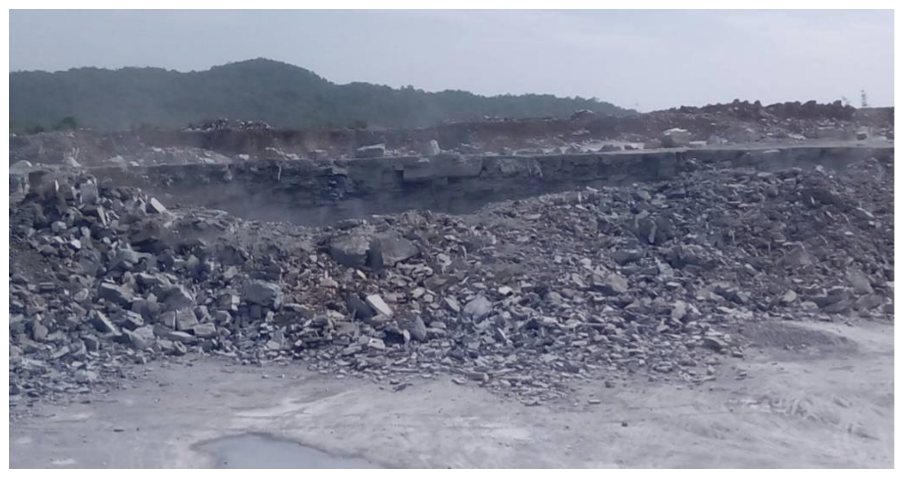
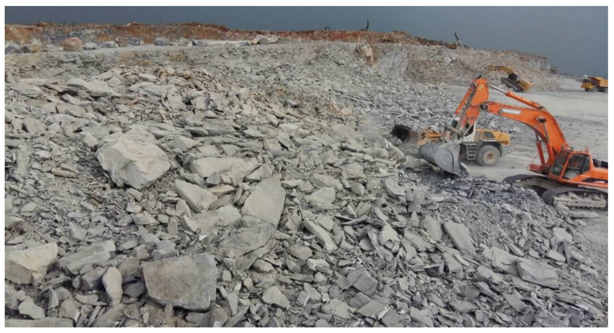
3.5. Case Study and Data Collection
4. Model Development
4.1. Hybridization of PSO-ANN
- Personal experiences of individuals that give their best results.
- Experiences of other individuals that give the best results of the entire swarms.
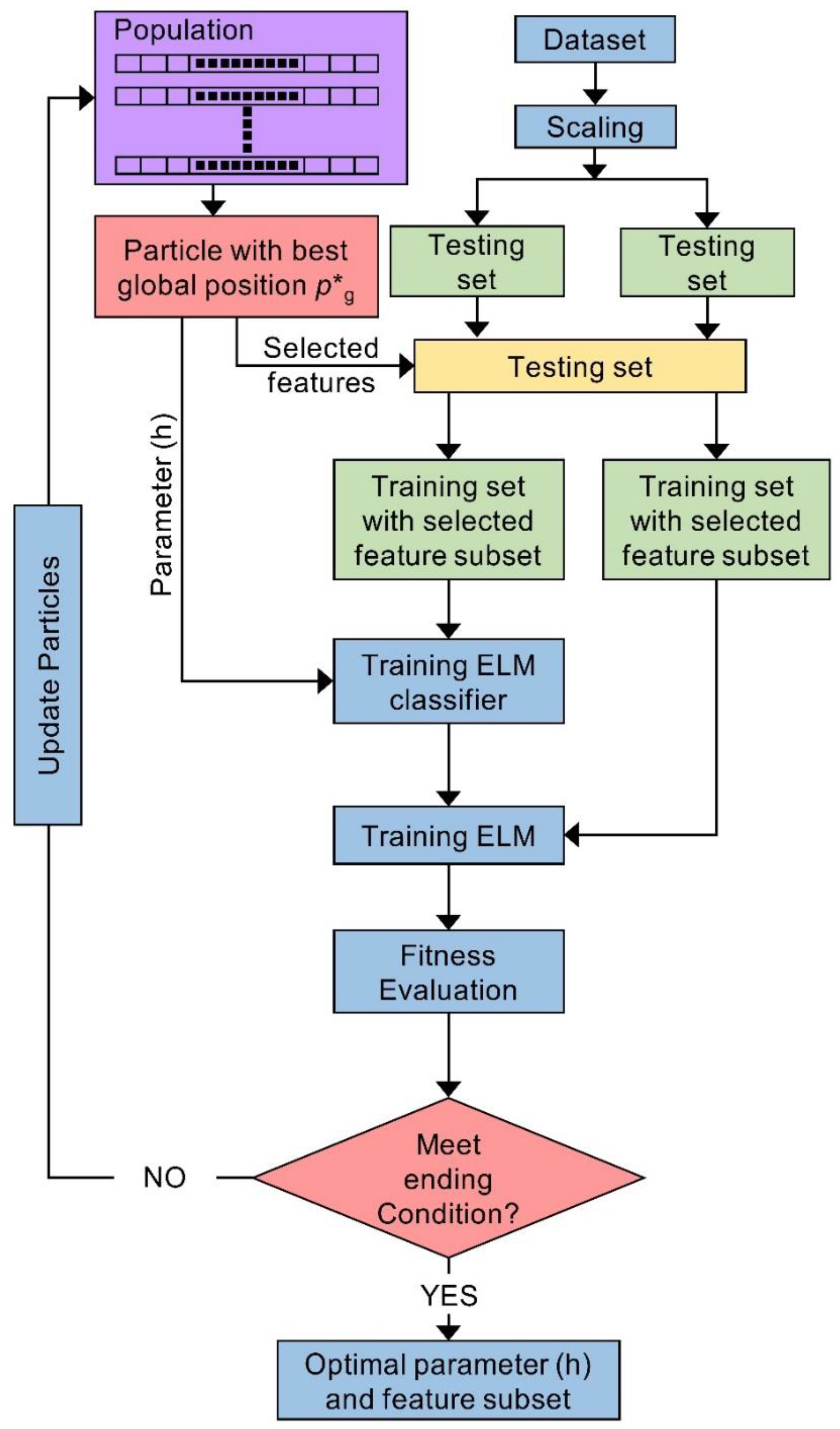
4.2. Hybridization of PSO-ELM
4.3. Hybridization of EO-ELM
| Algorithm 1: The algorithm of EO-ELM. Exponential term (F), λ is a turnover rate and defined as a random vector in between 0 and 1, a2 is used to control the exploitation task. a1 is used to control the exploration task, component consequences the direction of intensification and diversification of particles, r is defined as a random vector in between 0 and 1, generation rate (G), r1, and r2 denote the random values between 0 and 1. GCP is called generation rate control parameter |
| 1. Select training and testing dataset 2. Begin ELM training 3. Set hidden units of ELM 4. Obtain the number of input weights and hidden biases 5. Initialize the populations (P) 6. Initialize the fitness of four equilibrium candidates 7. Assignment of EO parameters value (a1 = 2, a2 = 1, GP = 0.5) 8. for it = 1 to maximum iteration number do 9. for i = 1 to P do 10. Estimate the fitness of the ith particle 11. if fitness () < fitness () 12. Replace fitness () with fitness () and with 13. elseif fitness () < fitness () & fitness () < fitness () 14. Replace fitness () with fitness () and with 15. elseif fitness () < fitness () & fitness () < fitness () & fitness () < fitness () 16. Replace fitness () with fitness () and with 17. elseif fitness () < fitness () & fitness () < fitness () & fitness () < fitness () & fitness () < fitness () 18. Replace fitness () with fitness () and with 19. end if 20. end for 21. = 22. (Equilibrium pool) 23. Allocate 24. for i = 1 to P do 25. Random generation of vectors and 26. Random selection of equilibrium candidate from equilibrium pool 27. Evaluate 28. Evaluate 29. Evaluate 30. Evaluate 31. (Concentration update) 32. end for 33. end for 34. Set ELM optimal input weights and hidden biases using 35. Obtain output weights 36. ELM testing |
4.4. Model Verification and Evaluation
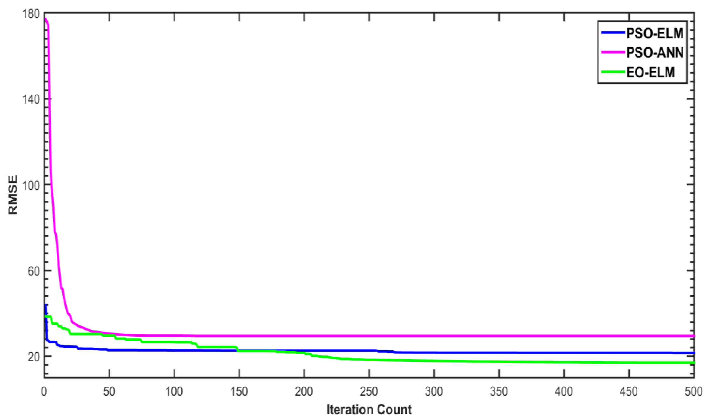
5. Results and Discussion
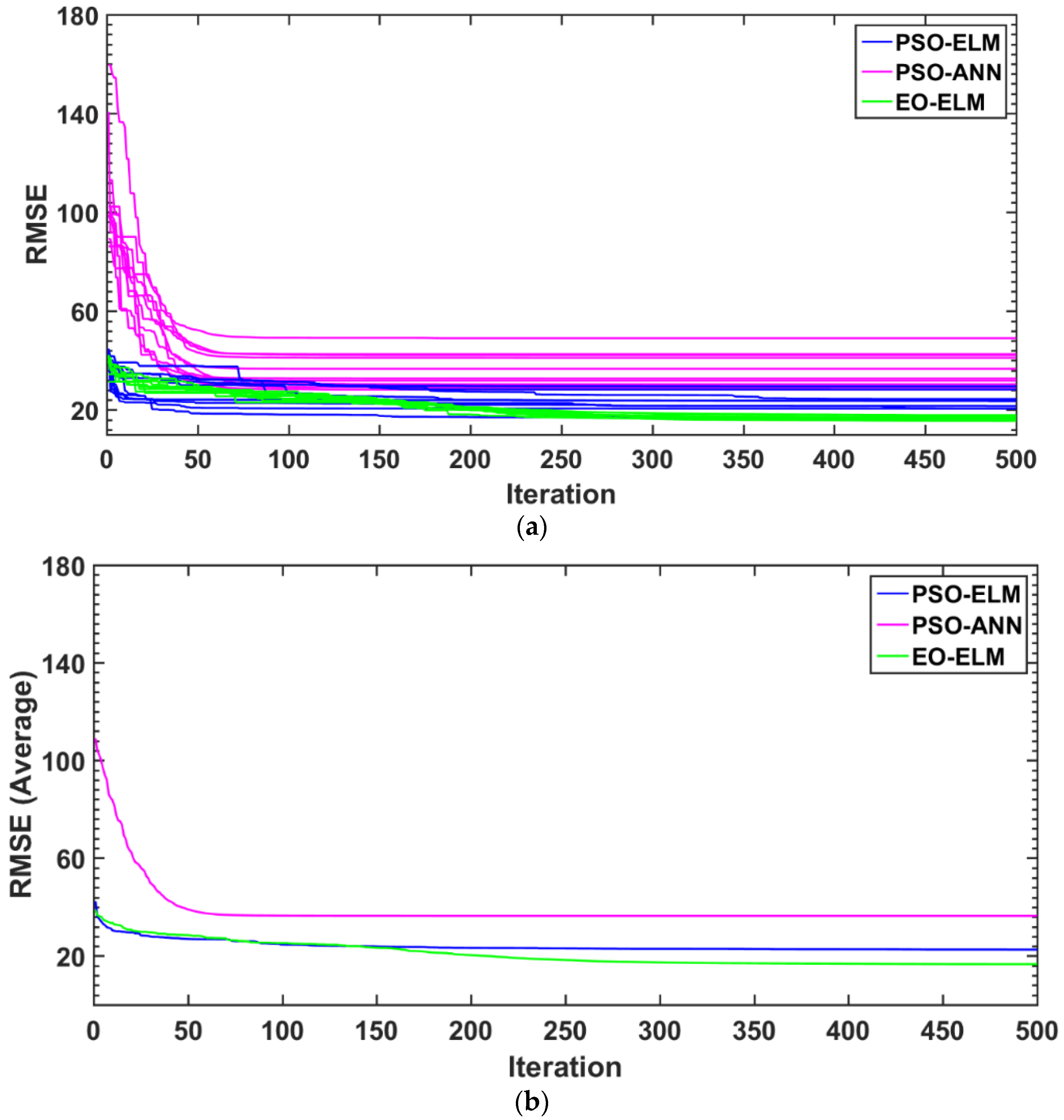
5.1. Average Performance of Models
5.2. Anderson–Darling (A–D) Test
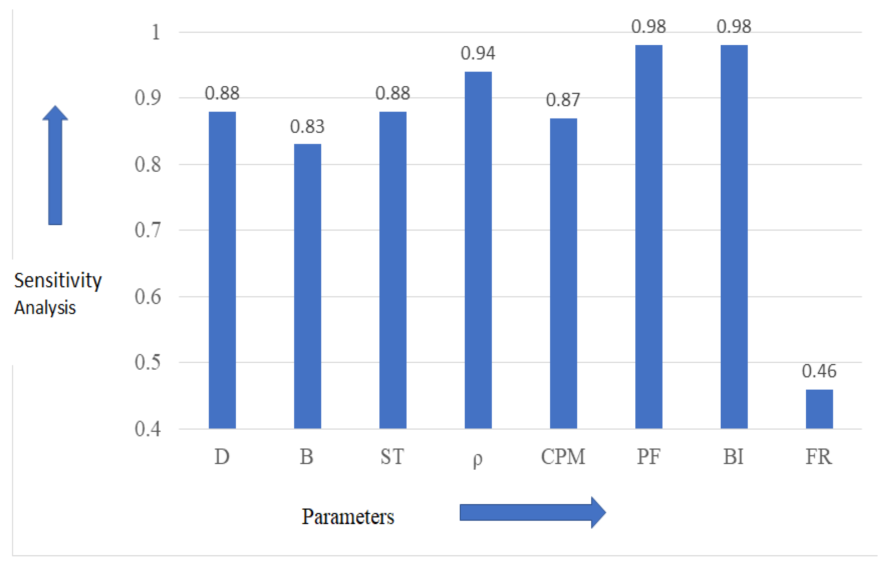
5.3. Sensitivity Analysis
6. Conclusions
Author Contributions
Funding
Institutional Review Board Statement
Informed Consent Statement
Data Availability Statement
Acknowledgments
Conflicts of Interest
References
- Bhandari, S. Engineering Rock Blasting Operations. Available online: https://www.osti.gov/etdeweb/biblio/661808 (accessed on 3 September 2022).
- Roy, P.P. Rock Blasting: Effects and Operations; IBH Publishing: New Delhi, India; Oxford, UK, 2005. [Google Scholar]
- Mohamad, E.T.; Yi, C.S.; Murlidhar, B.R.; Saad, R. Effect of Geological Structure on Flyrock Prediction in Construction Blasting. Geotech. Geol. Eng. 2018, 36, 2217–2235. [Google Scholar] [CrossRef]
- Li, H.B.; Zhao, J.; Li, J.R.; Liu, Y.Q.; Zhou, Q.C. Experimental studies on the strength of different rock types under dynamic compression. Int. J. Rock Mech. Min. Sci. 2004, 41, 68–73. [Google Scholar] [CrossRef]
- Khandelwal, M.; Singh, T.N. Prediction of blast-induced ground vibration using artificial neural network. Int. J. Rock Mech. Min. Sci. 2009, 46, 1214–1222. [Google Scholar] [CrossRef]
- Raina, A.K.; Murthy, V.M.S.R.; Soni, A.K. Estimating flyrock distance in bench blasting through blast induced pressure measurements in rock. Int. J. Rock Mech. Min. Sci. 2015, 76, 209–216. [Google Scholar] [CrossRef]
- Bhatawdekar, R.M.; Edy, M.T.; Danial, J.A. Building information model for drilling and blasting for tropically weathered rock. J. Mines Met. Fuels 2019, 67, 494–500. [Google Scholar]
- Mohamad, E.T.; Murlidhar, B.R.; Armaghani, D.J.; Saad, R.; Yi, C.S. Effect of Geological Structure and Blasting Practice in Fly Rock Accident at Johor, Malaysia. J. Teknol. 2016, 78. [Google Scholar] [CrossRef]
- Sastry, V.R.; Chandar, K.R. Assessment of objective based blast performance: Ranking system. In Measurement and Analysis of Blast Fragmentation; CRC Press: New Delhi, India, 2009; pp. 13–17. [Google Scholar]
- Kanchibotla, S.S.; Valery, W.; Morrell, S. Modelling fines in blast fragmentation and its impact on crushing and grinding. In Explo ’99—A Conference on Rock Breaking; The Australasian Institute of Mining and Metallurgy: Kalgoorlie, Australia, 1999; pp. 137–144. [Google Scholar]
- Armaghani, D.J. Rock fragmentation prediction through a new hybrid model based on imperial competitive algorithm and neural network. Smart Constr. Res. 2018, 2, 1–12. [Google Scholar] [CrossRef]
- Thornton, D.; Kanchibotla, S.S.; Brunton, I. Modelling the Impact of Rockmass and Blast Design Variation on Blast Fragmentation. Fragblast 2002, 6, 169–188. [Google Scholar] [CrossRef]
- Cunningham, C.V.B. The Kuz-Ram fragmentation model–20 years on. In Brighton Conference Proceedings; European Federation of Explosives Engineer: Brighton, UK, 2005; Volume 2005, pp. 201–210. [Google Scholar]
- Venkatesh, H.S.; Bhatawdekar, R.M.; Adhikari, G.R.; Theresraj, A.I. Assessment and Mitigation of Ground Vibrations and Flyrock at a Limestone Quarry. 1999, pp. 145–152. Available online: https://www.academia.edu/34145884/ASSESSMENT_AND_MITIGATION_OF_GROUND_VIBRATIONS_AND_FLYROCK_AT_A_LIMESTONE_QUARRY (accessed on 3 September 2022).
- Raina, A.K.; Chakraborty, A.K.; Choudhury, P.B.; Sinha, A. Flyrock danger zone demarcation in opencast mines: A risk based approach. Bull. Eng. Geol. Environ. 2011, 70, 163–172. [Google Scholar] [CrossRef]
- Xiong, H.; Yin, Z.Y.; Nicot, F. A multiscale work-analysis approach for geotechnical structures. Int. J. Numer. Anal. Methods Geomech. 2019, 43, 1230–1250. [Google Scholar] [CrossRef]
- Xiong, H.; Yin, Z.Y.; Nicot, F. Programming a micro-mechanical model of granular materials in Julia. Adv. Eng. Softw. 2020, 145, 102816. [Google Scholar] [CrossRef]
- Xiong, H.; Yin, Z.Y.; Zhao, J.; Yang, Y. Investigating the effect of flow direction on suffusion and its impacts on gap-graded granular soils. Acta Geotech. 2021, 16, 399–419. [Google Scholar] [CrossRef]
- Xiong, H.; Wu, H.; Bao, X.; Fei, J. Investigating effect of particle shape on suffusion by CFD-DEM modeling. Constr. Build. Mater. 2021, 289, 123043. [Google Scholar] [CrossRef]
- Chen, F.; Xiong, H.; Wang, X.; Yin, Z. Transmission effect of eroded particles in suffusion using CFD-DEM coupling method. Acta Geotech. 2022, 1–20. [Google Scholar] [CrossRef]
- Fu, Y.; Zeng, D.; Xiong, H.; Li, X.; Chen, Y. Seepage effect on failure mechanisms of the underwater tunnel face via CFD-DEM coupling. Comput. Geotech. 2020, 121, 103449. [Google Scholar] [CrossRef]
- Xiong, H.; Yin, Z.Y.; Nicot, F.; Wautier, A.; Marie, M.; Darve, F.; Veylon, G.; Philippe, P. A novel multi-scale large deformation approach for modelling of granular collapse. Acta Geotech. 2021, 16, 2371–2388. [Google Scholar] [CrossRef]
- Wang, X.; Yin, Z.Y.; Xiong, H.; Su, D.; Feng, Y.T. A spherical-harmonic-based approach to discrete element modeling of 3D irregular particles. Int. J. Numer. Methods Eng. 2021, 122, 5626–5655. [Google Scholar] [CrossRef]
- Wang, X.; Yin, Z.Y.; Zhang, J.Q.; Xiong, H.; Su, D. Three-dimensional reconstruction of realistic stone-based materials with controllable stone inclusion geometries. Constr. Build. Mater. 2021, 305, 124240. [Google Scholar] [CrossRef]
- Chen, G.; Li, Q.-Y.; Li, D.-Q.; Wu, Z.-Y.; Liu, Y. Main frequency band of blast vibration signal based on wavelet packet transform. Appl. Math. Model. 2019, 74, 569–585. [Google Scholar] [CrossRef]
- Li, Q.-Y.; Chen, G.; Luo, D.-Y.; Ma, H.-P.; Liu, Y. An experimental study of a novel liquid carbon dioxide rock-breaking technology. Int. J. Rock Mech. Min. Sci. 2020, 128, 104244. [Google Scholar] [CrossRef]
- Hudaverdi, T.; Akyildiz, O. A new classification approach for prediction of flyrock throw in surface mines. Bull. Eng. Geol. Environ. 2019, 78, 177–187. [Google Scholar] [CrossRef]
- Kecojevic, V.; Radomsky, M. Flyrock phenomena and area security in blasting-related accidents. Saf. Sci. 2005, 43, 739–750. [Google Scholar] [CrossRef]
- Bajpayee, T.S.; Rehak, T.R.; Mowrey, G.L.; Ingram, D.K. Blasting injuries in surface mining with emphasis on flyrock and blast area security. J. Saf. Res. 2004, 35, 47–57. [Google Scholar] [CrossRef] [PubMed]
- Adhikari, G.R. Studies on Flyrock at Limestone Quarries. Rock Mech. Rock Eng. 1999, 32, 291–301. [Google Scholar] [CrossRef]
- Raina, A.K.; Murthy, V.M.S.R.; Soni, A.K. Flyrock in bench blasting: A comprehensive review. Bull. Eng. Geol. Environ. 2014, 73, 1199–1209. [Google Scholar] [CrossRef]
- Hasanipanah, M.; Amnieh, H.B. A Fuzzy Rule-Based Approach to Address Uncertainty in Risk Assessment and Prediction of Blast-Induced Flyrock in a Quarry. Nat. Resour. Res. 2020, 29, 669–689. [Google Scholar] [CrossRef]
- Bhatawdekari, R.M.; Danial, J.A.; Edy, T.M. A review of prediction of blast performance using computational techniques. In Proceedings of the ISERME 2018 International Symposium on Earth Resources Management & Environment, Thalawathugoda, Sri Lanka, 24 August 2018. [Google Scholar]
- Sharma, L.K.; Vishal, V.; Singh, T.N. Developing novel models using neural networks and fuzzy systems for the prediction of strength of rocks from key geomechanical properties. Measurement 2017, 102, 158–169. [Google Scholar] [CrossRef]
- Koohmishi, M. Assessment of strength of individual ballast aggregate by conducting point load test and establishment of classification method. Int. J. Rock Mech. Min. Sci. 2021, 141, 104711. [Google Scholar] [CrossRef]
- Monjezi, M.; Bahrami, A.; Varjani, A.Y.; Sayadi, A.R. Prediction and controlling of flyrock in blasting operation using artificial neural network. Arab. J. Geosci. 2011, 4, 421–425. [Google Scholar] [CrossRef]
- Ghasemi, E.; Amini, H.; Ataei, M.; Khalokakaei, R. Application of artificial intelligence techniques for predicting the flyrock distance caused by blasting operation. Arab. J. Geosci. 2014, 7, 193–202. [Google Scholar] [CrossRef]
- Dehghani, H.; Ataee-Pour, M. Development of a model to predict peak particle velocity in a blasting operation. Int. J. Rock Mech. Min. Sci. 2011, 48, 51–58. [Google Scholar] [CrossRef]
- Armaghani, D.J.; Mahdiyar, A.; Hasanipanah, M.; Faradonbeh, R.S.; Khandelwal, M.; Amnieh, H.B. Risk Assessment and Prediction of Flyrock Distance by Combined Multiple Regression Analysis and Monte Carlo Simulation of Quarry Blasting. Rock Mech. Rock Eng. 2016, 49, 3631–3641. [Google Scholar] [CrossRef]
- Marto, A.; Hajihassani, M.; Armaghani, D.J.; Mohamad, E.T.; Makhtar, A.M. A Novel Approach for Blast-Induced Flyrock Prediction Based on Imperialist Competitive Algorithm and Artificial Neural Network. Sci. World J. 2014. [Google Scholar] [CrossRef] [PubMed]
- Jahed Armaghani, D.; Hajihassani, M.; Monjezi, M.; Mohamad, E.T.; Marto, A.; Moghaddam, M.R. Application of two intelligent systems in predicting environmental impacts of quarry blasting. Arab. J. Geosci. 2015, 8, 9647–9665. [Google Scholar] [CrossRef]
- Trivedi, R.; Singh, T.N.; Gupta, N. Prediction of Blast-Induced Flyrock in Opencast Mines Using ANN and ANFIS. Geotech. Geol. Eng. 2015, 33, 875–891. [Google Scholar] [CrossRef]
- Hasanipanah, M.; Armaghani, D.J.; Amnieh, H.B.; Majid, M.Z.A.; Tahir, M.M.D. Application of PSO to develop a powerful equation for prediction of flyrock due to blasting. Neural Comput. Appl. 2017, 28, 1043–1050. [Google Scholar] [CrossRef]
- Faradonbeh, R.S.; Armaghani, D.J.; Amnieh, H.B.; Mohamad, E.T. Prediction and minimization of blast-induced flyrock using gene expression programming and firefly algorithm. Neural Comput. Appl. 2018, 29, 269–281. [Google Scholar] [CrossRef]
- Kumar, N.; Mishra, B.; Bali, V. A Novel Approach for Blast-Induced Fly Rock Prediction Based on Particle Swarm Optimization and Artificial Neural Network. In Proceedings of International Conference on Recent Advancement on Computer and Communication; Springer: Berlin/Heidelberg, Germany, 2018; Volume 34, pp. 19–27. [Google Scholar] [CrossRef]
- Rad, H.N.; Bakhshayeshi, I.; Jusoh, W.A.W.; Tahir, M.M.; Foong, L.K. Prediction of Flyrock in Mine Blasting: A New Computational Intelligence Approach. Nat. Resour. Res. 2020, 29, 609–623. [Google Scholar] [CrossRef]
- Koopialipoor, M.; Fallah, A.; Armaghani, D.J.; Azizi, A.; Mohamad, E.T. Three hybrid intelligent models in estimating flyrock distance resulting from blasting. Eng. Comput. 2019, 35, 243–256. [Google Scholar] [CrossRef]
- Kotsiantis, S.B.; Zaharakis, I.; Pintelas, P. Supervised machine learning: A review of classification techniques. Emerg. Artif. Intell. Appl. Comput. Eng. 2007, 160, 3–24. [Google Scholar]
- Blum, A.L.; Langley, P. Selection of relevant features and examples in machine learning. Artif. Intell. 1997, 97, 245–271. [Google Scholar] [CrossRef] [Green Version]
- Amini, H.; Gholami, R.; Monjezi, M.; Torabi, S.R.; Zadhesh, J. Evaluation of flyrock phenomenon due to blasting operation by support vector machine. Neural Comput. Appl. 2012, 21, 2077–2085. [Google Scholar] [CrossRef]
- Rad, H.N.; Hasanipanah, M.; Rezaei, M.; Eghlim, A.L. Developing a least squares support vector machine for estimating the blast-induced flyrock. Eng. Comput. 2018, 34, 709–717. [Google Scholar] [CrossRef]
- Lu, X.; Hasanipanah, M.; Brindhadevi, K.; Amnieh, H.B.; Khalafi, S. ORELM: A Novel Machine Learning Approach for Prediction of Flyrock in Mine Blasting. Nat. Resour. Res. 2020, 29, 641–654. [Google Scholar] [CrossRef]
- Jahed Armaghani, D.; Tonnizam Mohamad, E.; Hajihassani, M.; Alavi Nezhad Khalil Abad, S.V.; Marto, A.; Moghaddam, M.R. Evaluation and prediction of flyrock resulting from blasting operations using empirical and computational methods. Eng. Comput. 2016, 32, 109–121. [Google Scholar] [CrossRef]
- Ghasemi, E.; Sari, M.; Ataei, M. Development of an empirical model for predicting the effects of controllable blasting parameters on flyrock distance in surface mines. Int. J. Rock Mech. Min. Sci. 2012, 52, 163–170. [Google Scholar] [CrossRef]
- Gupta, R.N. Surface Blasting and Its Impact on Environment. Impact of Mining on Environment; Ashish Publishing House: New Delhi, India, 1980; pp. 23–24. [Google Scholar]
- Little, T.N. Flyrock risk. In Proceedings EXPLO; 2007; pp. 3–4. [Google Scholar]
- Richards, A.; Moore, A. Flyrock control-by chance or design. In Proceedings of the Annual Conference on Explosives and Blasting Technique; International Society for Environmental Ethics (ISEE), 2004; Volume 1, pp. 335–348. [Google Scholar]
- Trivedi, R.; Singh, T.N.; Raina, A.K. Prediction of blast-induced flyrock in Indian limestone mines using neural networks. J. Rock Mech. Geotech. Eng. 2014, 6, 447–454. [Google Scholar] [CrossRef]
- Zhou, J.; Aghili, N.; Ghaleini, E.N.; Bui, D.T.; Tahir, M.M.; Koopialipoor, M. A Monte Carlo simulation approach for effective assessment of flyrock based on intelligent system of neural network. Eng. Comput. 2020, 36, 713–723. [Google Scholar] [CrossRef]
- Lundborg, N.; Persson, A.; Ladegaard-Pedersen, A.; Holmberg, R. Keeping the lid on flyrock in open-pit blasting. Eng. Min. J. 1975, 176, 95–100. [Google Scholar]
- Roth, J. A Model for the Determination of Flyrock Range as a Function of Shot Conditions; National Technical Information Service: Alexandria, VA, USA, 1979. [Google Scholar]
- Stojadinović, S.; Pantović, R.; Žikić, M. Prediction of flyrock trajectories for forensic applications using ballistic flight equations. Int. J. Rock Mech. Min. Sci. 2011, 48, 1086–1094. [Google Scholar] [CrossRef]
- Bui, X.-N.; Nguyen, H.; Le, H.-A.; Bui, H.-B.; Do, N.-H. Prediction of Blast-induced Air Over-pressure in Open-Pit Mine: Assessment of Different Artificial Intelligence Techniques. Nat. Resour. Res. 2020, 29, 571–591. [Google Scholar] [CrossRef]
- Kasabov, N.; Scott, N.M.; Tu, E.; Marks, S.; Sengupta, N.; Capecci, E.; Othman, M.; Doborjeh, M.G.; Murli, N.; Hartono, R.; et al. Evolving spatio-temporal data machines based on the NeuCube neuromorphic framework: Design methodology and selected applications. Neural Netw. 2016, 78, 1–14. [Google Scholar] [CrossRef] [PubMed] [Green Version]
- Hajihassani, M.; Armaghani, D.J.; Marto, A.; Mohamad, E.T. Ground vibration prediction in quarry blasting through an artificial neural network optimized by imperialist competitive algorithm. Bull. Eng. Geol. Environ. 2015, 74, 873–886. [Google Scholar] [CrossRef]
- Roy, B.; Singh, M.P. An empirical-based rainfall-runoff modelling using optimization technique. Int. J. River Basin Manag. 2020, 18, 49–67. [Google Scholar] [CrossRef]
- Roy, B.; Singh, M.P.; Singh, A. A novel approach for rainfall-runoff modelling using a biogeography-based optimization technique. Int. J. River Basin Manag. 2021, 19, 67–80. [Google Scholar] [CrossRef]
- Kumar, R.; Singh, M.P.; Roy, B.; Shahid, A.H. A Comparative Assessment of Metaheuristic Optimized Extreme Learning Machine and Deep Neural Network in Multi-Step-Ahead Long-term Rainfall Prediction for All-Indian Regions. Water Resour. Manag. 2021, 35, 1927–1960. [Google Scholar] [CrossRef]
- Zhou, J.; Koopialipoor, M.; Murlidhar, B.R.; Fatemi, S.A.; Tahir, M.M.; Armaghani, D.J.; Li, C. Use of Intelligent Methods to Design Effective Pattern Parameters of Mine Blasting to Minimize Flyrock Distance. Nat. Resour. Res. 2020, 29, 625–639. [Google Scholar] [CrossRef]
- Murlidhar, B.R.; Armaghani, D.J.; Mohamad, E.T. Intelligence Prediction of Some Selected Environmental Issues of Blasting: A Review. Open Constr. Build. Technol. J. 2020, 14, 298–308. [Google Scholar] [CrossRef]
- Armaghani, D.J.; Hasanipanah, M.; Mahdiyar, A.; Majid, M.Z.A.; Amnieh, H.B.; Tahir, M.M.D. Airblast prediction through a hybrid genetic algorithm-ANN model. Neural Comput. Appl. 2018, 29, 619–629. [Google Scholar] [CrossRef]
- Murlidhar, B.R.; Kumar, D.; Armaghani, D.J.; Mohamad, E.T.; Roy, B.; Pham, B.T. A Novel Intelligent ELM-BBO Technique for Predicting Distance of Mine Blasting-Induced Flyrock. Nat. Resour. Res. 2020, 29, 4103–4120. [Google Scholar] [CrossRef]
- Faradonbeh, R.S.; Hasanipanah, M.; Amnieh, H.B.; Armaghani, D.J.; Monjezi, M. Development of GP and GEP models to estimate an environmental issue induced by blasting operation. Environ. Monit. Assess. 2018, 190, 351. [Google Scholar] [CrossRef]
- Anand, A.; Suganthi, L. Forecasting of Electricity Demand by Hybrid ANN-PSO Models. In Deep Learning and Neural Networks: Concepts, Methodologies, Tools, and Applications; IGI Global: Hershey, PA, USA, 2020; pp. 865–882. [Google Scholar] [CrossRef]
- Armaghani, D.J.; Hajihassani, M.; Mohamad, E.T.; Marto, A.; Noorani, S.A. Blasting-induced flyrock and ground vibration prediction through an expert artificial neural network based on particle swarm optimization. Arab. J. Geosci. 2014, 7, 5383–5396. [Google Scholar] [CrossRef]
- Cai, W.; Yang, J.; Yu, Y.; Song, Y.; Zhou, T.; Qin, J. PSO-ELM: A Hybrid Learning Model for Short-Term Traffic Flow Forecasting. IEEE Access 2020, 8, 6505–6514. [Google Scholar] [CrossRef]
- Zeng, J.; Roy, B.; Kumar, D.; Mohammed, A.S.; Armaghani, D.J.; Zhou, J.; Mohamad, E.T. Proposing several hybrid PSO-extreme learning machine techniques to predict TBM performance. Eng. Comput. 2021, 1–17. [Google Scholar] [CrossRef]
- Kaloop, M.R.; Kumar, D.; Zarzoura, F.; Roy, B.; Hu, J.W. A wavelet—Particle swarm optimization—Extreme learning machine hybrid modeling for significant wave height prediction. Ocean Eng. 2020, 213, 107777. [Google Scholar] [CrossRef]
- Cui, D.; Huang, G.-B.; Liu, T. ELM based smile detection using Distance Vector. Pattern Recognit. 2018, 79, 356–369. [Google Scholar] [CrossRef]
- Hoerl, A.E.; Kennard, R.W. Ridge Regression: Biased Estimation for Nonorthogonal Problems. Technometrics 2000, 42, 80. [Google Scholar] [CrossRef]
- Bartlett, P.L. The sample complexity of pattern classification with neural networks: The size of the weights is more important than the size of the network. IEEE Trans. Inf. Theory 1998, 44, 525–536. [Google Scholar] [CrossRef]
- Faramarzi, A.; Heidarinejad, M.; Stephens, B.; Mirjalili, S. Equilibrium optimizer: A novel optimization algorithm. Knowl. Based Syst. 2020, 191, 105190. [Google Scholar] [CrossRef]
- Nazaroff, W.W.; Alvarez-Cohen, L. Environmental Engineering Science; John Wiley & Sons: New York, NY, USA, 2001. [Google Scholar]
- Guo, Z. Review of indoor emission source models. Part 1. Overview. Environ. Pollut. 2002, 120, 533–549. [Google Scholar] [CrossRef] [PubMed]
- Kennedy, J.; Eberhart, R. Particle Swarm Optimization. In Proceedings of the ICNN’95—International Conference on Neural Networks, Perth, Australia, 27 November–1 December 1995; Volume 4, pp. 1942–1948. [Google Scholar] [CrossRef]
- Tangchawal, S. Planning and Evaluation for Quarries: Case Histories in Thailand; IAEG2006: Nottingham, UK, 2006. [Google Scholar]
- Jahed Armaghani, D.; Shoib, R.S.N.S.B.R.; Faizi, K.; Rashid, A.S.A. Developing a hybrid PSO–ANN model for estimating the ultimate bearing capacity of rock-socketed piles. Neural Comput. Appl. 2017, 28, 391–405. [Google Scholar] [CrossRef]
- Huang, G.-B.; Chen, L.; Siew, C.-K. Universal Approximation Using Incremental Constructive Feedforward Networks with Random Hidden Nodes. IEEE Trans. Neural Netw. 2006, 17, 879–892. [Google Scholar] [CrossRef] [PubMed]
- Zhu, H.; Tsang, E.C.C.; Zhu, J. Training an extreme learning machine by localized generalization error model. Soft Comput. 2018, 22, 3477–3485. [Google Scholar] [CrossRef]
- Mohapatra, P.; Chakravarty, S.; Dash, P.K. An improved cuckoo search based extreme learning machine for medical data classification. Swarm Evol. Comput. 2015, 24, 25–49. [Google Scholar] [CrossRef]
- Liu, H.; Mi, X.; Li, Y. An experimental investigation of three new hybrid wind speed forecasting models using multi-decomposing strategy and ELM algorithm. Renew. Energy 2018, 123, 694–705. [Google Scholar] [CrossRef]
- Satapathy, P.; Dhar, S.; Dash, P.K. An evolutionary online sequential extreme learning machine for maximum power point tracking and control in multi-photovoltaic microgrid system. Renew. Energy Focus 2017, 21, 33–53. [Google Scholar] [CrossRef]
- Li, L.-L.; Sun, J.; Tseng, M.-L.; Li, Z.-G. Extreme learning machine optimized by whale optimization algorithm using insulated gate bipolar transistor module aging degree evaluation. Expert Syst. Appl. 2019, 127, 58–67. [Google Scholar] [CrossRef]
- Figueiredo, E.M.N.; Ludermir, T.B. Effect of the PSO Topologies on the Performance of the PSO-ELM. In Proceedings of the 2012 Brazilian Symposium on Neural Networks, Curitiba, Brazil, 20–25 October 2012; pp. 178–183. [Google Scholar] [CrossRef]
- Liu, D.; Li, G.; Fu, Q.; Li, M.; Liu, C.; Faiz, M.A.; Khan, M.I.; Li, T.; Cui, S. Application of Particle Swarm Optimization and Extreme Learning Machine Forecasting Models for Regional Groundwater Depth Using Nonlinear Prediction Models as Preprocessor. J. Hydrol. Eng. 2018, 23. [Google Scholar] [CrossRef]
- Wang, Y.; Tang, H.; Wen, T.; Ma, J. A hybrid intelligent approach for constructing landslide displacement prediction intervals. Appl. Soft Comput. 2019, 81, 105506. [Google Scholar] [CrossRef]
- Kaloop, M.R.; Kumar, D.; Samui, P.; Gabr, A.R.; Hu, J.W.; Jin, X.; Roy, B. Particle Swarm Optimization Algorithm-Extreme Learning Machine (PSO-ELM) Model for Predicting Resilient Modulus of Stabilized Aggregate Bases. Appl. Sci. 2019, 9, 3221. [Google Scholar] [CrossRef]
- Armaghani, D.J.; Kumar, D.; Samui, P.; Hasanipanah, M.; Roy, B. A novel approach for forecasting of ground vibrations resulting from blasting: Modified particle swarm optimization coupled extreme learning machine. Eng. Comput. 2021, 37, 3221–3235. [Google Scholar] [CrossRef]
- Li, G.; Kumar, D.; Samui, P.; Nikafshan Rad, H.; Roy, B.; Hasanipanah, M. Developing a New Computational Intelligence Approach for Approximating the Blast-Induced Ground Vibration. Appl. Sci. 2020, 10, 434. [Google Scholar] [CrossRef]
- Cao, J.; Lin, Z.; Huang, G.-B. Self-Adaptive Evolutionary Extreme Learning Machine. Neural Process. Lett. 2012, 36, 285–305. [Google Scholar] [CrossRef]
- Chen, S.; Shang, Y.; Wu, M. Application of PSO-ELM in electronic system fault diagnosis. In Proceedings of the 2016 IEEE International Conference on Prognostics and Health Management (ICPHM), Ottawa, ON, Canada, 20–22 June 2016; pp. 1–5. [Google Scholar] [CrossRef]
- Huang, G.-B.; Zhu, Q.-Y.; Siew, C.-K. Extreme learning machine: A new learning scheme of feedforward neural networks. In Proceedings of the 2004 IEEE International Joint Conference on Neural Networks (IEEE Cat. No. 04CH37541), Budapest, Hungary, 25–29 July 2004; pp. 985–990. [Google Scholar]


| Parameters | Hole Diameter | Burden | Stemming Length | Rock Density | Charge per M | Powder Factor | Blastability Index | Weathering Index | Flyrock |
|---|---|---|---|---|---|---|---|---|---|
| Symbol | D | B | ST | ρ | CPM | PF | BI | WI | FR |
| Unit | mm | m | m | Cum.t | kg/m | kg/cum | % | Ratio | m |
| Minimum | 76 | 2.5 | 1.2 | 1.8 | 4.54 | 0.08 | 18.5 | 0.13 | 27 |
| Quartile1 | 76 | 2.7 | 2 | 1.8 | 4.99 | 0.19 | 28.6 | 0.25 | 37 |
| Average | 90 | 3 | 2 | 2 | 7 | 0.30 | 43 | 0.76 | 81 |
| Quartile3 | 102 | 3.6 | 2.95 | 2.5 | 8.99 | 0.40 | 54.6 | 0.88 | 82 |
| Maximum | 102 | 4.6 | 4 | 2.5 | 9.4 | 0.50 | 80.8 | 0.99 | 436 |
| Model | Parameters | Value |
|---|---|---|
| EO-ELM | Maximum Iteration | 500 |
| Size of Population | 25 | |
| a1 | 2.5 | |
| a2 | 2.5 | |
| GP | 0.6 | |
| PSO-ELM | Maximum Iteration | 500 |
| Size of Population | 25 | |
| C1 | 1 | |
| C2 | 2 | |
| W (inertia weight) | 0.9 | |
| PSO-ANN | Maximum Iteration | 500 |
| Size of Population | 25 | |
| C1 | 1 | |
| C2 | 2 | |
| W | 0.98 |
| Model | Training Data | Testing Data |
|---|---|---|
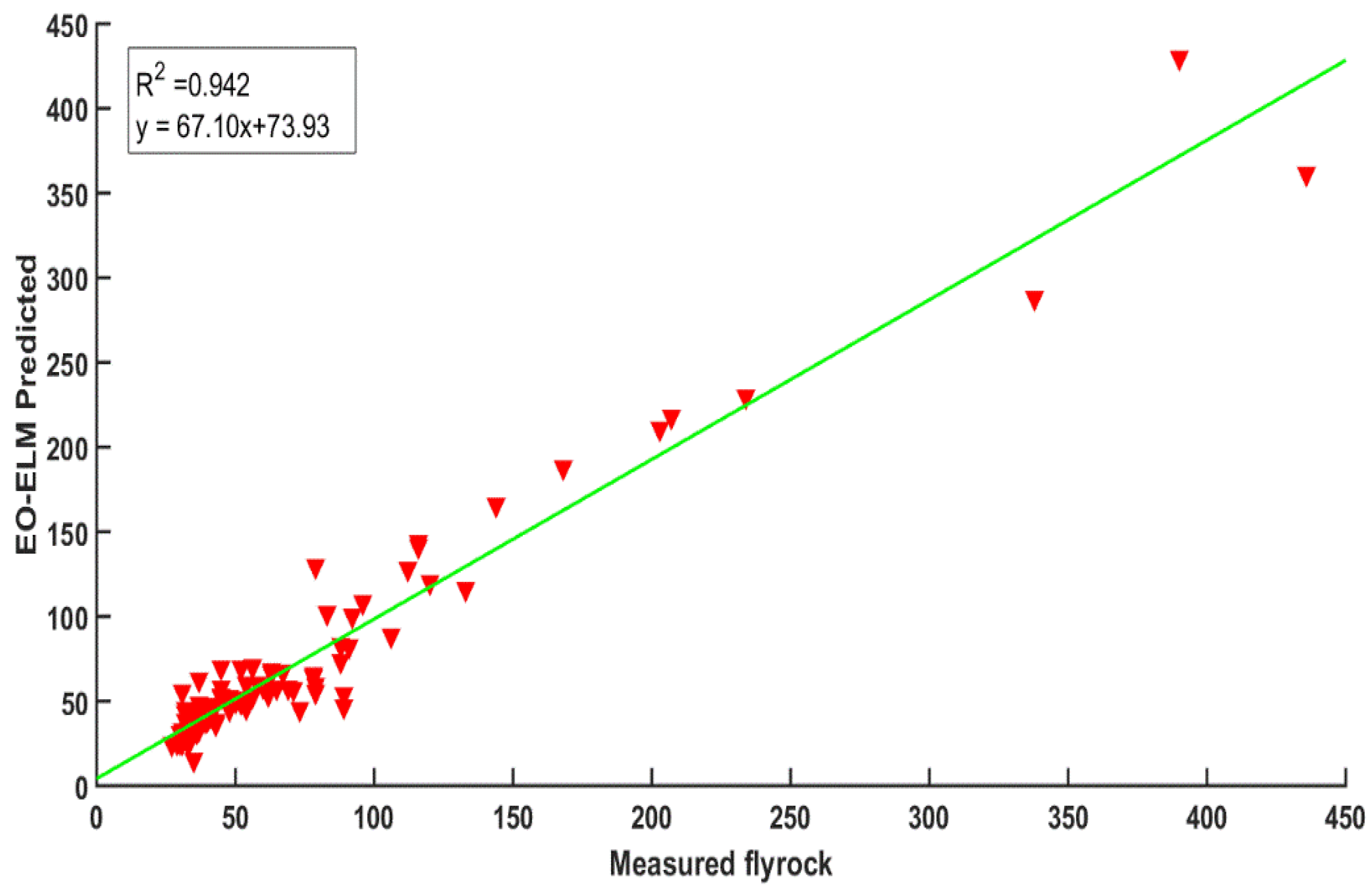
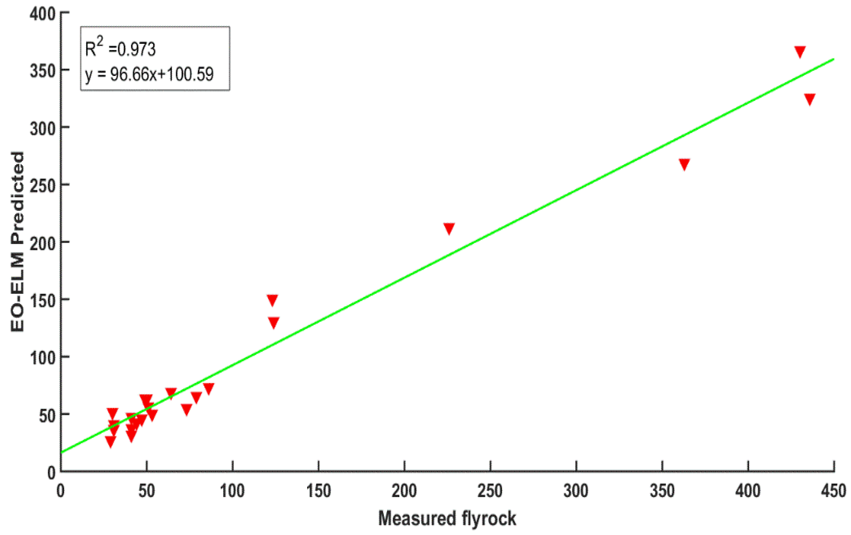
| EO-ELM | 67.10x + 73.93 | 96.66x + 100.59 |
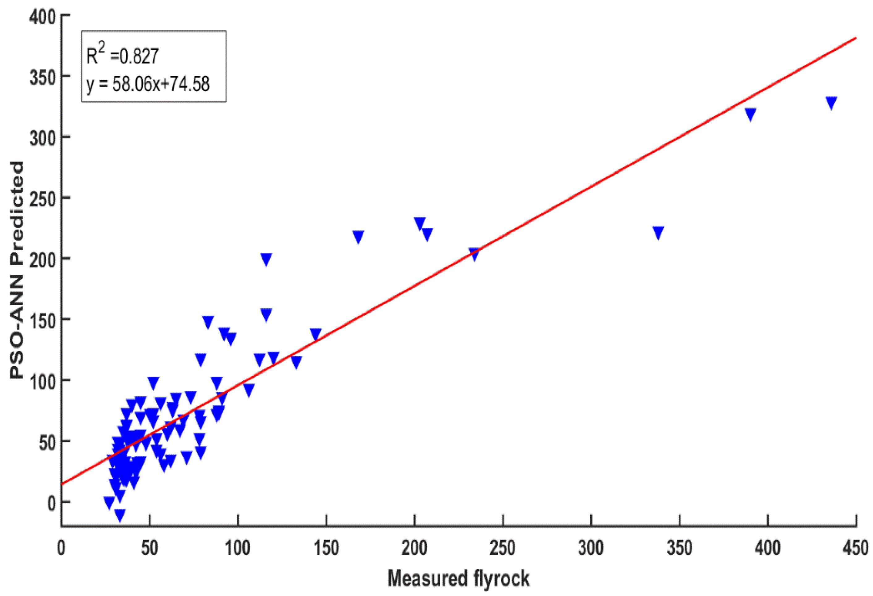
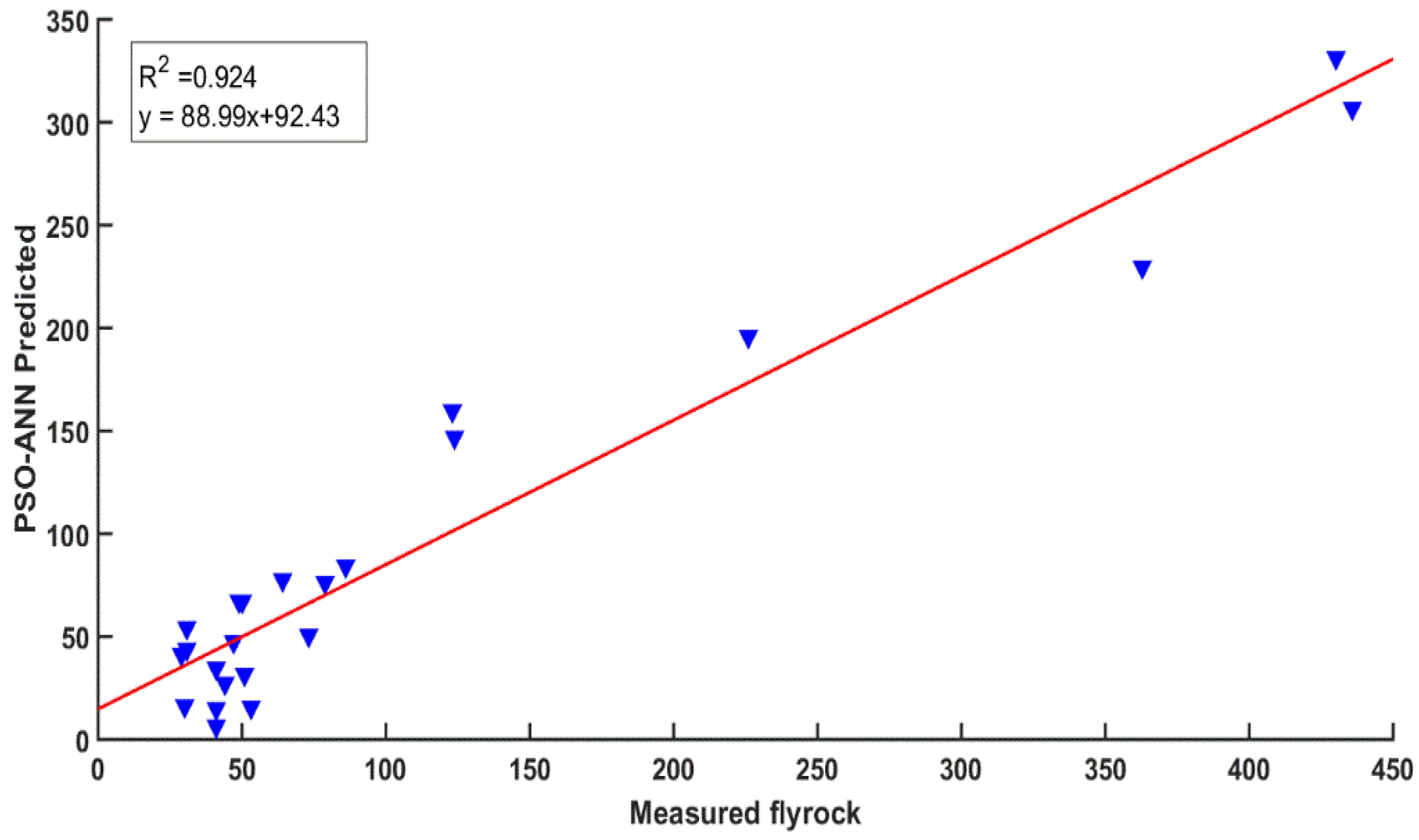
| PSO-ANN | 58.06x + 74.58 | 88.9x + 92.43 |
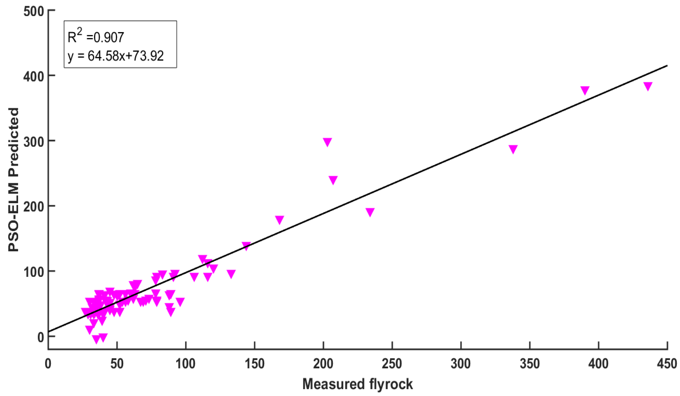
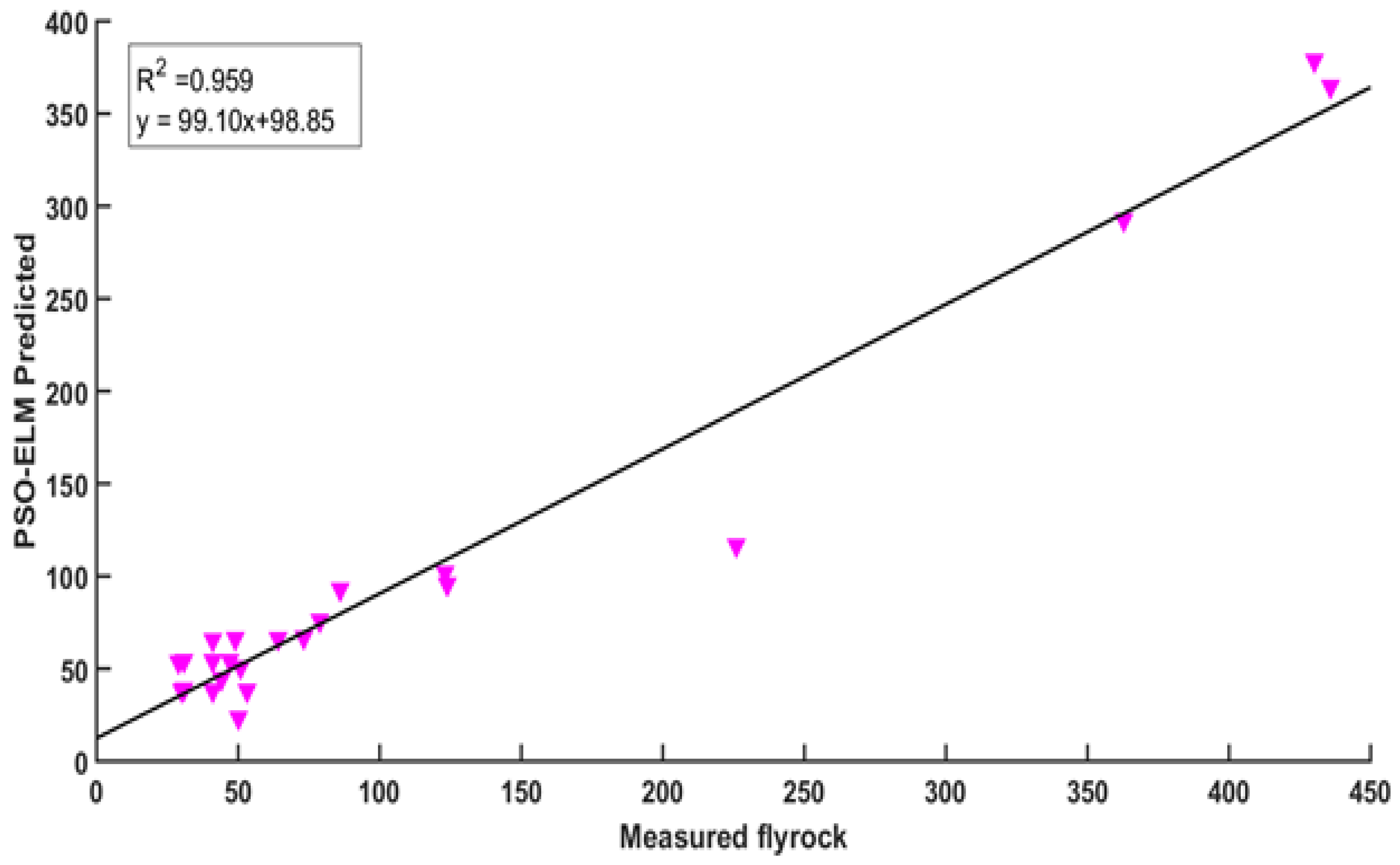
| PSO-ELM | 64.58x + 73.92 | 99.10x + 98.85 |
| Training Data Sets | |||||||
| R2 | RMSE | MAE | MAPE | NSE | VAF | A20 | |
| EO-ELM | 0.942 | 17.02 | 11.26 | 21.20 | 0.946 | 94.62 | 0.53 |
| PSO-ANN | 0.827 | 29.5 | 21.07 | 27.04 | 0.821 | 82.19 | 0.43 |
| PSO-ELM | 0.907 | 21.56 | 15.64 | 24.27 | 0.900 | 90.08 | 0.45 |
| Testing Data Sets (Continued) | |||||||
| R2 | RMSE | MAE | MAPE | NSE | VAF | A20 | |
| EO-ELM | 0.973 | 34.82 | 20.3 | 17.60 | 0.978 | 97.88 | 0.65 |
| PSO-ANN | 0.924 | 48.12 | 31.68 | 24.25 | 0.93 | 92.89 | 0.35 |
| PSO-ELM | 0.959 | 35.7 | 23.53 | 21.84 | 0.96 | 95.79 | 0.56 |
| Training Data Sets | |||||||
| R2 | RMSE | MAE | MAPE | NSE | VAF | A20 | |
| EO-ELM | 0.95 | 16.66 | 12.13 | 19.87 | 0.95 | 94.46 | 0.60 |
| PSO-ANN | 0.83 | 29.68 | 19.33 | 29.30 | 0.82 | 82.06 | 0.41 |
| PSO-ELM | 0.88 | 23.68 | 16.76 | 26.96 | 0.88 | 88.29 | 0.47 |
| Testing Data Sets (Continued) | |||||||
| R2 | RMSE | MAE | MAPE | NSE | VAF | A20 | |
| EO-ELM | 0.97 | 32.14 | 19.78 | 20.37 | 0.93 | 93.97 | 0.57 |
| PSO-ANN | 0.87 | 64.44 | 36.02 | 29.96 | 0.72 | 74.72 | 0.33 |
| PSO-ELM | 0.88 | 48.55 | 26.97 | 26.71 | 0.84 | 84.84 | 0.51 |
| Count | Mean | Median | SD | AD | p-Value | |
|---|---|---|---|---|---|---|
| Actual | 114 | 81.307 | 50.5 | 85.927 | 0 | 1 |
| PSO-ELM | 114 | 78.951 | 54.632 | 75.877 | 2.843 | 0.03244 |
| PSO-ANN | 114 | 78.183 | 55.035 | 70.484 | 2.308 | 0.00619 |
| EO-ELM | 114 | 79.311 | 53.492 | 76.092 | 0.8886 | 0.004215 |
Disclaimer/Publisher’s Note: The statements, opinions and data contained in all publications are solely those of the individual author(s) and contributor(s) and not of MDPI and/or the editor(s). MDPI and/or the editor(s) disclaim responsibility for any injury to people or property resulting from any ideas, methods, instructions or products referred to in the content. |
© 2023 by the authors. Licensee MDPI, Basel, Switzerland. This article is an open access article distributed under the terms and conditions of the Creative Commons Attribution (CC BY) license (https://creativecommons.org/licenses/by/4.0/).
Share and Cite
Bhatawdekar, R.M.; Kumar, R.; Sabri Sabri, M.M.; Roy, B.; Mohamad, E.T.; Kumar, D.; Kwon, S. Estimating Flyrock Distance Induced Due to Mine Blasting by Extreme Learning Machine Coupled with an Equilibrium Optimizer. Sustainability 2023, 15, 3265. https://doi.org/10.3390/su15043265
Bhatawdekar RM, Kumar R, Sabri Sabri MM, Roy B, Mohamad ET, Kumar D, Kwon S. Estimating Flyrock Distance Induced Due to Mine Blasting by Extreme Learning Machine Coupled with an Equilibrium Optimizer. Sustainability. 2023; 15(4):3265. https://doi.org/10.3390/su15043265
Chicago/Turabian StyleBhatawdekar, Ramesh Murlidhar, Radhikesh Kumar, Mohanad Muayad Sabri Sabri, Bishwajit Roy, Edy Tonnizam Mohamad, Deepak Kumar, and Sangki Kwon. 2023. "Estimating Flyrock Distance Induced Due to Mine Blasting by Extreme Learning Machine Coupled with an Equilibrium Optimizer" Sustainability 15, no. 4: 3265. https://doi.org/10.3390/su15043265