1. Introduction
According to the World Cities Report 2022, published by United Nations-Habitat (UN-Habitat), the urban population, which is currently 56.2% of all humans, is expected to increase to 60.4% by 2030 and reach 68.4% by 2050, with two-thirds of all humans becoming urbanites [
1]. As suggested by Muggah (2021), “If the 19th and 20th centuries were the era of the state, the 21st century was the era of the city”, and considering how cities are responsible for more than 80% of the world’s GDP, such an increase in population in urban areas is no surprise [
2]. Until now, cities have always been pointed out as having chronic problems caused by excessive population concentration, such as housing shortages, transportation issues, health hygiene issues, crime, and poverty problems, but cities have continued to expand constantly.
In a modern society where the majority of the world’s population lives in cities, governments always have a duty and responsibility to keep the cities sustainable [
3]. For the continuous growth and management of the city, the choice of the state’s or government’s strategy, which includes policy measures, is very important. The issue of the distribution of urban land use has a long history, and the legitimacy of government intervention—particularly in land and housing—varies between countries, but has always been secured. Land use, a limited resource, must always be efficient and fair, because to lead to a livable city, various infrastructures and systematic management that can accommodate the city’s population and buildings are required. Because sustainable development cannot be achieved without significantly transforming the way we build and manage our urban spaces, these demands are not limited to specific countries [
4], but apply to all countries. The Sustainable Development Goals (SDGs), adopted by the United Nations in 2015, call for universal action to ensure that everyone enjoys peace and prosperity. The 11th goal is ‘sustainable cities and communities’. It states that some goals of the 11th SDG are to strengthen comprehensive and sustainable urbanization and capacity for participatory, integrated, and sustainable human settlement planning and management in all countries [
4].
Public-led urban development projects can be considered a form of direct government intervention because they physically improve the city. They are also known as essential and effective policy tools for sustainable urban growth. Governments in many countries have promoted various government-led urban development projects with the aim of improving the quality of the built environment in both large and relatively small areas according to the national and local conditions, in order to build the cities they want to live in through urban development projects.
Urban development projects have social, economic, and cultural impacts in many ways, as public authorities participate in them to physically improve cities. However, these effects have ambivalence. There is a gap in economic performance, such as per capita income and gross regional product; in social performance, such as levels of education, social services and cultural activities; and in the physical and spatial performance of transport infrastructure and environmental service facilities based on urban space. Such a gap can cause the uneven distribution of facilities and services across spatial units within the city. Nevertheless, these spatial changes induced by urban policies are highly sensitive to real estate, especially housing prices and rents.
As is well known, urban policies should be designed with great care because of the various socio-economic effects that are caused by urban policies. In particular, the increase in housing prices indicates that the city has improved, and it is likely that urban policies have shown physical improvement effects. Housing is an asset, but it is also an essential good for people to live in, and the burden of housing costs due to changes in property prices in turn hinders the sustainability of the city. To this end, many governments provide urban development projects and housing, such as affordable and social housing, but this does not help to alleviate the process of social segmentation and exclusion. Instead, they create wealthy islands near poor neighborhoods, making cities highly socio-economic and more mutually exclusive regional patchworks. To the extent that low-cost or social housing is included in the project, the low revenues of these target housing policies undermine the financial feasibility of the project and consequently require significant government support or subsidies.
The effectiveness of urban policy depends on the demographic and environmental characteristics of the city before the policy is implemented. Therefore, it is important to find out in what context and with what effect urban policy is implemented. Public-led land development projects vary according to the amount of public money invested. In particular, the size of the infrastructure installation and the price of the land in the residential area are again due to changes in the housing market in the area. Many point out that the main reason for the dilemma of public intervention is that only a small number of people benefit from public development.
The research problem of this study is to explore how public-led urban development projects, especially policies that supply housing, affect housing prices. Moreover, the impact will depend on the character of the development project. More objective analysis is required than ever for policies to create a sustainable city. Challenges regarding planning policies, new business models, as well as strategies and tools to measure or evaluate sustainability and reduce uncertainty in the implementation process require new analyses that cannot be limited to environmental analyses of sustainability [
5]. In particular, the application and implementation of SDG 11 in public-led urban development projects should be applied in different contexts to prioritize development, and this study proposes a complex and quantitative approach for this.
The objectives of this paper are as follows: First, the purpose in this paper is to clarify the impact of the regional and project characteristics of public-led housing site development projects on housing prices in the surrounding areas. The sample areas are classified into clusters based on various characteristic variables, such as the size of public funds invested at the time of project creation, the population and sociological characteristics of the project site, and cluster-based policy effects. Second, we suggest a methodology for analyzing regional-based policy effects from various angles. Specifically, this paper presents a three-stage policy evaluation methodology by utilizing SOM, DID, and LSTM.
Accordingly, this study empirically analyses samples of different sizes of public funds, project sites, and regional characteristics invested at the time of project creation. Therefore, by comprehensively considering various factors, this study aims to identify various characteristics of public-led development policies and to find out a balance between equity and efficiency. Moreover, this paper proposes a methodology to evaluate urban policies from different perspectives. Most existing urban policy evaluation methodologies rely mainly on a multilinear regression model for policy impact analysis, but the impact of urban policies has not been made clear in the long term, so there have been analytical limitations on the impact. Given the need to measure and predict both long and short-term effects towards sustainable urban development, this study focuses on two models as policy evaluation methodologies. These approaches are expected to be applied to various policy evaluation methodologies in the future.
The empirical analysis in this paper focuses on cases in South Korea. However, the relevance for an international audience is plausible. South Korea has experienced rapid urbanization, and a variety of policies have been implemented for the efficient development of urban land. In particular, the Housing Site Development Project, which is the subject of this study, has been promoted in a short period of time as a government-led housing site supply policy. There are several countries and cities that have also considered the use of public land development strategies [
6,
7]. The results of this study will have implications globally. Furthermore, many countries can make advanced decisions on how to appropriately apply such sustainable development strategies in the future.
The paper is structured as follows: The next section presents previous studies with theoretical reflection on relevant planning and policy theory literatures. The theoretical section is followed by an elaboration of the methodological choices that are the basis of the case study analysis.
Section 4 shows the results of the analysis. The concluding section discusses the theoretical and practical implications of the empirical findings and suggests avenues for future research.
3. Materials and Methods
This section consists of four parts. First, the sites of the housing site development projects—each sample subject to this study—are described in detail. And then, three research methodologies—SOM, DID, and LSTM—are explained. Subsequently, the data and variable settings are explained, and finally, we explain an overview of the overall analysis methodology.
3.1. Selection of the Sample Area
The primary purpose of this study is to analyze the impact of housing site development projects on housing prices in surrounding areas. The process of selecting 69 project sites for the study is as follows: Among 78 housing site development areas that disclosed construction cost data, the area where the project was completed as of 2023 while the data was available before completion of the project was selected. However, Jeju Island was excluded from the sample area because the heterogeneity of housing markets between the island and peninsula was large. The final selected business areas are a total of 68 residential site development project areas, and
Figure 1 below shows the location of each project. The size of the circle represents the size of the housing site development project.
Looking at the characteristics of the entire sample, the smallest site is located in Mokpo, with an area of 85.151 million , and the largest workplace is located in Hwaseong, Gyeonggi-do, with 24,014.896 million . The average area of the sample area was 241,247,000 , with a standard deviation of 3629.045 . Housing site development projects are located mostly in Gyeonggi-do, surrounding Seoul, and are generally distributed in existing cities or areas neighboring them. It can be understood that this is due to the characteristics of the project, aiming to solve the urgent housing shortage in urban areas.
3.2. Methodology
3.2.1. Clustering for Regional Analysis
Cluster analysis, or clustering, is a technique that classifies similar data into the same group without prior knowledge of the group [
47,
48]. Clusters are organized to have maximum similarity within the group and minimum similarity between different groups. It is widely used in various fields such as sales, stocks, exchange rates, weather, and biomedical measurement.
The ultimate purpose of this study is to provide standards of policy evaluation based on regional characteristics. The first thing that is needed in order to analyze regional characteristics or to present basis for policy proposals is regional classification using cluster analysis. Since the reliability of cluster analysis results depends on the algorithm used [
49], it is very important to choose an appropriate methodology. The self-organizing map (SOM), developed by Teuvo Kohonen, is a machine learning technique used in various fields such as image analysis, text classification, and behavioral pattern analysis, and has attracted attention for its applicability and excellence in cluster analysis [
50,
51,
52].
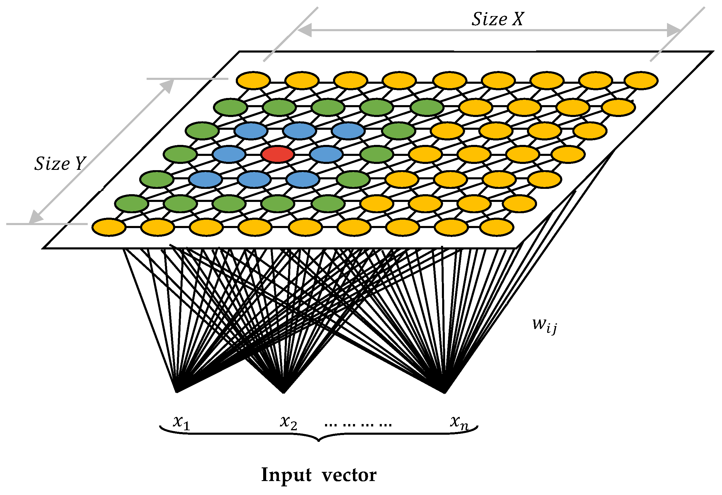
A self-organizing map (SOM) is a type of artificial neural network (ANN) that is trained using unsupervised learning to produce a low-dimensional (typically two-dimensional), discretized representation of the input space of training samples, called a map, and is therefore a method for dimensionality reduction. Self-organizing maps (SOM) differ from other artificial neural networks in that they use competitive learning as opposed to error-correcting learning, such as backpropagation with gradient descent; in that, they use a neighborhood function to preserve the topological properties of the input space. The
Figure 2 is the visualized format of SOM. SOM identifies each characteristic of the sample, such as yellow, green, blue, and red circles as
,
,
, and
, respectively. SOM also represents the concept of clustering by grouping similar features together. As such, SOM can be used to cluster high-dimensional data sets by performing a dimensionality reduction and then visualizing the clustering in the form of maps.
Each data point in the data set recognizes itself by competing for representation. Self-organizing mapping starts from initializing the weight vectors. Then, a sample vector is randomly selected, and the map of weight vectors is searched to find the weight that best represents that sample. Each weight vector has neighboring weights that are close to it. The chosen weight is rewarded by being able to become more like the randomly chosen sample vector. The neighbors of that weight are also rewarded by being able to become more like the chosen sample vector.
Because the SOM results are in map form and follow Tobler’s first law of geography—the basic assumption of geography—it is easy for geographers to understand the clusters created as a result of SOM [
53]. Therefore, in this study, groups were classified using SOM, and analysis was conducted according to the group.
3.2.2. Difference in Difference (DID)
To this end, the prices of housing transactions have been used as an indirect indicator to express the changes in the local housing market caused by the impact of the policy, since the price fluctuation can indicate the improvement of the housing environment in terms of supply and demand. On the other hand, revealing the effectiveness of a policy requires separating the ‘treatment’ and ‘control’ groups to remove the general effect of change over time. In other words, since the policy effect may be distorted by external factors other than whether the policy is applied or not, care must be taken in the analysis. An empirical analysis was carried out using the difference-in-difference (DID) model.
The DID Is a methodology that measures the performance of the policy by dividing the experimental group and the comparison group according to the application of policy; the group to which the policy is applied is called the treat group, and the group to which it is not applied is called the control group. In addition, in order to compare the effects before and after the application of the policy project, the analysis is conducted separately before and after the application of the policy project [
54].
Let denote the average selling price per square meter of a house at time point t of area i. In an area with i = 0 (around the project site), t = 0 indicates before the housing site development project is implemented, and t = 1 is after the housing site development project is carried out. In the project site, where t = 1, t = 0 means before the project is implemented, and t = 1 means after the project is implemented.
Using this notation method, represents the average price of houses in the project area observed after the completion of the housing development project, and represents the difference between the average price of houses in the project site and the surrounding area after the housing site development project.
However, the formula
or
cannot show the effect of the housing site development project on the average price of houses in the surrounding area. This is because the difference in housing prices between the two points in time is affected not only by whether the policy is applied, but also by other situational differences. In addition, the difference in housing prices between the two regions is determined not only by the difference in the improvement effect of the housing site development project, but also by the difference in income, population density, and land prices between regions. This can also be expressed as ‘
policy effect
regional effect’. Therefore, in order to know the effects of urban regeneration projects, macroeconomic effects or regional effects other than policy effects must be removed [
55]. The difference-in-difference method eliminates them in the following way:
The first term on the right-hand side of Equation (1) above represents the price change between time points in the location of the housing development project, and the second term represents the price change between time points in the surrounding region. If the housing prices in the two regions are affected by macroeconomic factors to the same extent, the macroeconomic effect that caused the difference between the time points before and after the implementation of the project in the housing site development project area is expected to have caused the same difference between the time points before and after the implementation of the project in the surrounding area. Therefore, by differentiating the difference between the two regions, the effect of macro factors on house prices can be removed, and only the pure policy effect can be estimated. DID can also be expressed in the form of a simple regression, as shown in Equation (2):
refers to the price of the house (i) at time (t). is a dummy variable representing before and after the completion of the housing site development project, and is a dummy variable representing whether the housing site development project was applied. In the above OLS estimation equation, the estimate representing the policy effect is D, which is the coefficient value of the and interaction terms.
3.2.3. Specification of Long Short-Term Memory (LSTM)
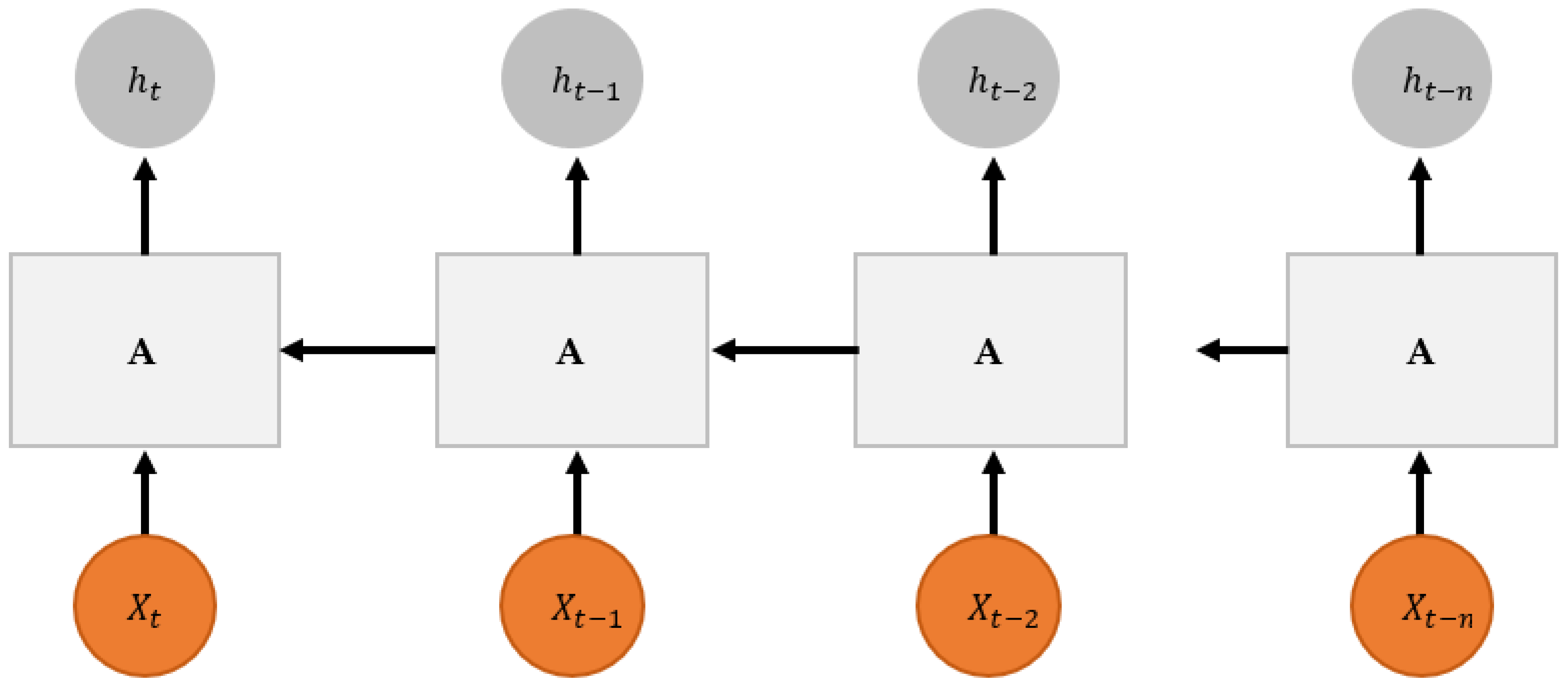
RNN is used to reveal the relationship between current output data and historical information. Existing fully connected neural networks (Fully Connected Layers) and convolutional neural networks (CNNs) require a process that passes through the input layer, the hidden layer, and the output layer. Each layer is either fully connected or partially connected. However, there is no connection between current and past learning, so there is a limit to sequential data learning. RNN, on the other hand, remembers past information [
55].
Figure 3 is the visualized format of RNN.
It uses this to predict the current output value. Therefore, the hidden layers of the RNN are connected and contain not only the current input layer, but also the output value of the previous hidden layer. Recurrent neural networks (RNNs) are algorithms that process ordered sequence data or effectively model time series data because they are trained through the backpropagation algorithmic process (BPTT) over time [
56].
LSTM is a special form of RNN model that can solve long-term dependence problems [
57,
58]. As described above, RNN has the disadvantage that the impact of previous long-distance learning on current outcomes becomes insignificant as sequential data is lengthened. On the other hand, LSTM uses a structure called a memory cell, which can store existing input values and solve this long-term dependence problem. Therefore, LSTM can perform relatively well in long data tasks [
59].
Every RNN has an iterative neural network module in the form of a chain, and its structure exists in a simple form. LSTM also has the same structure, but the internal repetition module has a relatively different structure. Unlike a single neural network layer, LSTM interacts in a way that has four kinds of modules. In
Figure 4, LSTM is a special network structure with three ‘gates’.
The ‘gate’ of the LSTM plays an important role in selectively influencing the state of each time point. It is a structure in which the fully connected network layer using the sigmoid activation function outputs a value between 0 and 1, so that when the gate is opened (sigmoid output 1) and closed (sigmoid output 0), it carries no information. If the above LSTM configuration diagram is expressed as an equation, it can be expressed as Equation (3).
The values follow the arrows and go through the LSTM information: the forget gate (
), input gate (
), and output gate (
). There are two activation functions at the gates, the first of which is the sigmoid function, denoted as ‘
’, which outputs a value between 1 and 0 to control whether a value should flow through the gates. Then, there is the hyperbolic tangent function denoted as “
tanh”, which outputs a value between −1 and 1, giving a weighting to the representation of their relative importance. “
W” and “
b” represent the weightage and bias for the respective gate.
3.3. Data Acquisition and Database Construction
This study consists of two stages of analysis. Among them, the first step is to cluster the sample area based on the characteristics of the region and the project. The data acquisition and data curation processes for SOM analysis corresponding to the first step are as follows: An area is a space that is produced differentially according to its demographic, social, economic, and environmental characteristics.
The core of SOM analysis is to cluster individual business sites based on variables found to affect housing prices for housing-site development projects. To this end, urban environment variables affecting housing prices revealed in previous studies were adopted as variables in SOM analysis.
Specifically, demographic factors affect the construction or value of a house [
60,
61,
62,
63,
64,
65], and the size of the population determines the supply and demand of housing. Housing prices may follow a steeper upward trajectory as population density increases [
66].
On the other hand, the inventory of houses already supplied in the housing market and the formed housing price are important factors that determine the housing market. This is because the fluctuations in housing prices by region can be largely explained by the characteristics of the residential environment [
33].
In addition, traditionally, the land use environment has been found to have a significant impact on housing prices. In particular, various studies on land-use regulation have shown that a decrease in housing supply causes a decrease in housing prices when the ratio of housing sites decreases, which leads to an increase in housing prices [
67,
68,
69].
In order to achieve the purpose of the study, it is necessary to consider the economic and regional characteristics of the housing site development project. It is expected that the policy effect will differ depending on the size of the public cost invested in the housing site development project. In addition, the location variable was also considered by considering the X and Y coordinates together. Through this, six domains were finally selected: population, housing, real estate market, built (land use) environment, project scale, and location.
Twenty datasets were used, including various population data, such as population ratio by age and household ratio, and land-use data (see
Table 2).
The core of SOM analysis is to cluster individual business sites based on the variables found to affect housing prices for housing-site development projects. To this end, urban environment variables (see
Section 2.2) affecting housing prices revealed in previous studies were adopted as variables in SOM analysis.
The study unit of analysis was defined as the municipal-level divisions in South Korea, namely si (city), gun (county), and gu (district). Each of these local units has its own upper-level local government (i.e., si, metropolitan city, or do, province), and each district has different policies. Since the housing site development districts are designated on a scale of more than 100,000 , it is necessary to adopt cities, counties, and districts as the target regional units of this study in order to derive accurate policy effects.
A region is a space that is produced differently according to its population, social, ecological, and environmental characteristics. As the purpose of this study is to examine the effectiveness of policies based on regional characteristics, these regional characteristics were taken into account. To this end, 16 datasets were used, including various population data such as population, population density, population growth rate, household ratio, distribution of housing type, property price, and land use data.
To test the hypothesis that the size of the project represents the effectiveness of the policy in a different way, Pro1 and Pro2 variables are added, corresponding to the explanatory variables of the project. Each variable represents the share of infrastructure installation costs in total project costs per unit and in total project costs.
In the SOM clustering analysis, geographic coordinates need to be considered in regard to spatial aspects. The most basic way to do this is to construct spatial coordinates variably, like other variables. However, since each project site is represented as a polygon, spatial coordinates that can be represented are needed, and the X and Y coordinates of the center point were calculated and used as spatial variables.
In particular, in the analysis method by machine learning algorithms, including SOM, if the scale of the characteristics of each data point is severely different, the data pattern cannot be found, which can lead to serious errors in the analysis. In order to solve the problem that each variable is different in units and categories within the built dataset, a normalization operation was performed to unify the data into the same category. Through the normalization process, all data have a value of 0 to 1, and the normalized value represents the relative position of the original data value within the variable. To normalize all data, this study performed a commonly used minimum–maximum normalization calculation. The equation is as follows:
The second step is to evaluate the validity of the policy. DID and LSTM were adopted to see how the housing site development project affects housing prices. Among them, the data for the DID analysis corresponding to the regression analysis model are shown in the table below. The dependent variable set for DID analysis is the apartment transaction price per unit, and the actual transaction price data provided by the Ministry of Land, Infrastructure, and Transport (MOLIT) were used as the data. The data include the prices of individual housing transactions and the characteristics of houses, and it is the most commonly used data for various analyses of the impact of housing prices in Korea. In order to control variables affecting housing transactions regarding transacted apartment floors in the building, we subtracted the construction year of the transacted apartment from the year of transaction of traded houses provided in the relevant data; these were set as control variables. Variable description illustrate in
Table 3.
Finally, the housing price index data provided by KB Kookmin Bank (hereinafter referred to as “KB”) were adopted as data for LSTM analysis to predict future housing market prices in the area where the housing site development project was implemented. KB calculates a regional price index based on appraisal prices. The price index is established by regularly evaluating individual house prices and calculating the price index through the market capitalization flow of the housing market produced, using the appraisal price per house as the base price. The KB housing price index provides monthly house price data by subdividing them into municipal-level divisions. The data have been collected since 1986. Since the index has been collected for almost 40 years, it is regarded to show high validity for various time series and machine learning analyses related to housing prices.
3.4. Methodological Outline
The purpose of this study is to identify the impact of housing site development projects on housing prices and to present policy implications according to the regional characteristics and business characteristics of each project. To this end, three analyses were conducted sequentially using the data described (See
Section 3.2).
First, SOM was carried out using regional data and housing site development project data. In this SOM analysis, which clusters similar project sites, a total of four clusters were created. Then, these four clusters are used for both DID and LSTM analysis. The purpose is to measure the exact validity of the policy through DID analysis, and the results of DID analysis can confirm whether the housing price in each cluster area was affected by the housing price compared to the surrounding area. On the other hand, it is possible to predict changes in housing prices in housing development project areas through LSTM analysis. Predicting which public-led projects will be affected in the long term is important in policy evaluation. Through this analysis, it is possible to confirm the sustainability of regional urban development policies and see what regional characteristics can be predicted. The above process is schematically illustrated in
Figure 5 below.
4. Result and Discussion
4.1. Result of SOM and Characteristics by Cluster
To comprehensively examine the effects of housing site development projects through cluster analysis, this study reduced multidimensional data to two-dimensional data using SOM, and then performed cluster analysis using the K-means technique [
52]. The K-means algorithm, which belongs to machine learning unsupervised learning, is simply a clustering algorithm that combines data into K clusters. It is significant to distinguish groups that collect data with similar characteristics. Therefore, PCA has a limitation in that it is difficult to find the vector with the largest distribution of data and analyze the meaning of the axis because the vector with the largest distribution cannot always express the characteristics of the data well. In addition, the appropriate grid shape and size must be selected. Two types of lattice forms, square (four adjacent cells) or hexagonal (six adjacent cells), are often used in the form of the lattice [
52], and hexagonal grids were used in this study. The map size can be selected by the subjectivity of the researcher, but in most cases, it is determined by the ‘optimal visualization scale’ according to the size of the input dataset [
70], so a 4 × 4 grid was used in this study.
The SOM was applied to classify 69 project areas into areas with similar regional and project characteristics. As a result of SOM using sixteen regional characteristic variables, two business characteristic variables, and two coordinate variables, the project areas were classified into four clusters. The descriptive statistics for each cluster are shown in
Table 4.
Cluster 1 adopted a business area centered on the center of the metropolitan area. All three project sites in Seoul are included, and this area has a large population and a high population density. It is the area with the highest apartment ratio, and the rate of increase in housing prices was also higher than that of other clusters. Although it has the highest residential area ratio, it is the area with the lowest green area ratio, which is due to the characteristics of the metropolitan area. As land prices are concentrated in high-priced areas, the cost of the project is high, and the business area is not large. The characteristic feature is that, in addition to the housing site development project nearby, various small and large urban development projects have already been carried out before or at the same time. Cluster 2 was composed mainly of areas near the metropolitan area with a large total population. When comparing the period before and after the project, it is the region with the highest population growth rate. Compared to other regions, there are more multi-family houses, and the proportion of apartments is at a medium and low level. Although there were some variations in housing prices, they appeared at a medium to low level. Industrial areas accounted for a higher proportion than other clusters, and the proportion of infrastructure installation was higher than that of other regions. Cluster 2 is a place where housing site development projects have already been carried out in the surrounding areas over a certain period of time after large-scale urban development projects have already been carried out around large cities. Cluster 3 has the largest number of areas adopted, with a small population and a small population density. It was the cluster with the lowest proportion of apartments, and the cluster is mainly centered on local small cities with low housing prices. It is characterized by the low proportion of residential areas, the high proportion of green areas, and the high proportion of old buildings. As for the characteristics of the project, the project cost per area was low, and the proportion of infrastructure installation was low. Most of these areas have established projects in nearby areas, and the area and size of the project are larger than existing projects. In particular, the majority of the innovative cities were included in this cluster. Finally, cluster 4 is an area with a medium population, and shows a high population growth rate. It consists of small and medium-sized local cities that are somewhat far from the metropolitan area, and the population density was high. Although the ratio of apartments is high, the number of detached houses is high, real estate prices are low, and the rate of increase compared to the previous year is high. It is characterized by the high cost of the project and the high proportion of infrastructure installation costs. There are no other projects in the nearby area, and the area is formed mainly in the central city center. The summary of the main features of clusters by domain are shown in the
Table 5.
The results below are K-means clustering results for these four clusters. The data used in this study consist of a multidimensional data set with 20 variables, and K-means clustering visually represents data points according to two principal component coordinates by performing principal component analysis (PCA). PCA is significant in projecting existing data vectors by linearly transforming them. As a result of the analysis, Dim2 was 16.6%, Dim1 was 24.5%, and the distribution of each sample is shown in
Figure 6.
4.2. Analysis and Results of DID
Table 6 shows the result of the frequency analysis of each cluster. Each sample belongs to the treatment group if it is located within the housing site development project site, and to the control group if it is located in the surrounding area. In addition, based on the completion date of individual projects, the time variable was set to 0 if it was before the completion date and 1 if it was after. The temporal range is 6 months each before and after completion, and a one year period was set as the research range. The total number of samples selected through this process is 285,789, and the number of samples is shown in
Table 6 below.
The average housing price per square meter of Cluster 1 was 716.24 (±328.54) (10,000 won), slightly lower than comparison group’s 686.51 (±403.66) (10,000 won). The size of the house was 73.48 (±22.74) in the experimental group, which was somewhat smaller than 79.14 (±33.10) in the comparison group. In addition, the age of the building was 16.26 (±7.97) years in the experimental group, which was slightly lower than 21.71 (±9.63) years in the comparison group.
Meanwhile, in Cluster 2, the mean price of traded houses is 291.20 (±139.98) (10,000 won), and the mean price of the comparison group is 254.87 (±102.99) (10,000 won), indicating that the housing price was the lowest among all groups. On the other hand, the size of the traded houses was the largest, with the experimental group averaging 83.83 (±24.23)
, and the comparison group averaging 76.49 (22.79)
. The age of the building was also counted as 12.67 (±6.40) years in the experimental group and 15.92 (±6.33) years in the comparison group. In the case of Cluster 3, the housing price of the experimental group was 312.89 (±159.55) million won compared to the comparative group, which was higher than 274.21 (±135.04) million won, and the size of the house was 79.23 (±20.29)
, which was higher than the 73.18 (±24.44)
of the comparison group. The average age of the buildings was 16.32 (±8.58) and 19.69 (±8.56) years, respectively. Finally, in Cluster 4, the average housing price of the experimental group was 317.02 (±112.36) million won, and the average price of the comparison group was 298.09 (±165.55) million won. The size of the house in the experimental group was 80.73 (±23.14)
, the age of the building was 15.55 (±9.67) years, the size of the comparison group was 75.16 (±23.41)
, and the age of the building was 18.09 (±8.20) years. See Characteristics of subjects in
Table 7.
Table 8 reports the effect of the housing site development projects compared to the surrounding area. It also shows DID analysis with year and site fixed effects of each cluster. Except for Model 1, the time variable was positive, indicating that housing prices increased over time in all Models. However, in Model 1, the parameters are not statistically significant at the 5% level. Model 1 shows the effect of the housing site development program on the area of Cluster 1. The results suggest that housing prices are associated with a 2.9% increase in business areas. Models 2 and 4 also show that housing prices are associated with an increase in business areas of 3.7% and 5.5%, respectively. Model 3 shows the opposite. In the area of Cluster 3, house prices are observed to be 7.5% lower than in the surrounding area.
The main interest in this analysis is in the direction of the DID variable. If the DID variable has a positive direction, it means that the effect of the project appears to be a higher increase in housing prices than in the surrounding areas. As a result of the analysis, it was difficult to find a significant result in Models 1 and 4. Model 2 showed a positive (0.032) and statistically significant value at the 5% level. This means that apartment prices in the residential land development project area rose 3.2% more than those in the surrounding areas. On the other hand, in Model 3, the beta value of the DID variable was negative (−0.013) and statistically significant at the 10% level, indicating that apartments in the business area increased by 1.3% less than in the neighboring areas.
4.3. Analysis Results of LSTM
As noted in
Section 3.3, it is important in policy evaluation which public-led projects will be effective in the long term. Therefore, this study adopts a future prediction model using LSTM and uses it as a basis for comprehensive analysis, along with the difference-in-difference analysis in
Section 4.2.
First, the trend of all-time series data used before the analysis was shown by cluster. The left side of the
Figure 7 shows the apartment sales price index data for Cluster 1. In the case of Cluster 1, the data tended to increase in a form that was not largely distributed. This suggests that Cluster 1 is geographically close and belongs in a similar real estate market. Cluster 2 is somewhat distributed, but the trend is similar, and most prices have increased since 2012, confirming that there has been no significant change from 2012 to 2020. Cluster 2 started construction in 2003 for the earliest areas (sites 40 and 64) and in 2014 for the latest areas (site 35). Cluster 3 contains the largest number of samples, with the earliest regions being 2010 (sites 66, 67 and 68) and the latest being 2022 (site 01). Cluster 4 also showed a similar pattern to Cluster 3 with early areas in 2010 (sites 65) and late areas in 2020 (sites 04 and 06).
On the other hand, as shown at the very right side of the
Figure 7, which shows the average rate of increase in housing prices of each cluster, Cluster 1 showed a higher rate of change, and Cluster 2 showed a similar pattern to Cluster 1, as the rate of change has recently increased. Cluster 3 and Cluster 4 appear to have similar volatility.
This study used Tensorflow—a Python-based open-source software (Tensorflow 2.0 beta) widely used for multilayer neural network applications—to model house prices using LSTM, referencing various previous studies [
71,
72,
73]. The overall mechanism of the model was discussed in a previous section (see
Section 3.2.3); the details of the implementation of the LSTM model were presented here. There is no rule of thumb for optimizing neural networks; it is difficult to place relative importance on one thing over another [
71,
74]. Thus, the overall performance was evaluated using the root mean square error (RMSE) based on the previous literature [
71,
72,
73,
75,
76]. LSTM should determine hyper-parameters to optimize the model. In this study, three hidden layers, 1000 tests, full batch size, the activation function ReLU (Relu Function), and ADAM algorithms were used for optimization. RMSE was minimized by these hyper-parameters.
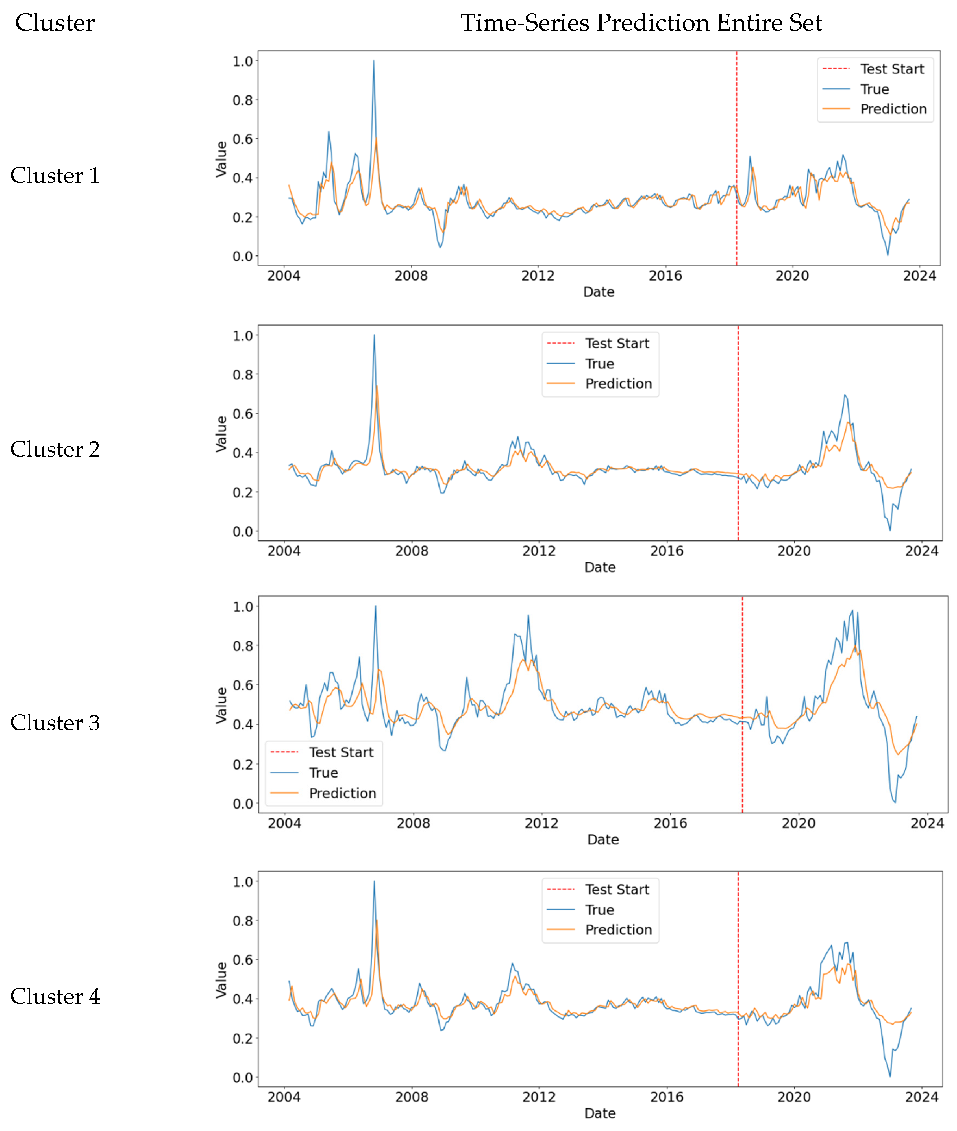
A total of four price prediction models were created using LSTM, which were optimized for each cluster. A total of 25% of the data was used in the forecast, equivalent to 60 months. The representations for each prediction are shown in
Figure 8. The RMSE values represent the performance of each final model, as shown in
Table 9.
The figure below shows the result of the LSTM model for the prediction of house prices for each of the clusters. In total, 60 out of 240 months were predicted, and 180 months were used for the test. In order to increase validity, the analysis was conducted starting in September 2018, when housing prices rose sharply nationwide. In this way, it is possible to examine the trends of housing prices by regional characteristics. First, in the case of Cluster 1, we found that the rate of increase rises in the short term, before stabilizing again and rising to a lower slope. The similarity between the predicted results and the actual data seems to be closer than for the other clusters. Moreover, in the case of Cluster 1, it can be interpreted together with the results of DID analysis. This combination of analysis shows that housing site development projects in these regions did not have significant impact on market prices. In addition, in the case of cluster 2, housing prices have entered a phase of rising housing prices since 2022, and the cross-sectional analysis has shown that it has some effect on the rise in housing prices in the region. The results of Cluster 3 have the opposite meaning, and the rise in housing prices in the areas with the highest rate of price increase among the four graphs supports the results of regression analysis, which would be expected to be more affected by other projects than the housing site development districts. Cluster 4 could not be interpreted with the results of DID analysis. However, Cluster 4 showed a modest upward trend, which did not affect housing prices; this could be interpreted as an upward trend in housing prices due to the improvement of the residential environment across the city.
4.4. Comprehensive Results
In this study, 69 regions were classified into four clusters using the SOM analysis method based on neural networks, which capture the unique characteristics of regions and companies. Areas in the same cluster are generally close to each other because they share geographical characteristics. However, even if the characteristics of the region or project are similar, they are classified in the same cluster.
Cluster 1 was an area with high housing prices in the central areas of the metropolitan area. The level of the project costs was moderate, and the proportion of infrastructure installation was low. The analysis of the impact of housing development projects in this cluster area compared to the surrounding area was not statistically significant. This can be attributed to the presence of numerous influential projects in the surrounding area, which is a result of the nature of the project area. In addition, the size of the project is not large. It is expected that housing prices in the area will continue to rise in the future. Therefore, it is important to promote additional projects that are suitable for the area, in addition to housing development projects. These projects should aim to alleviate the increasing burden of housing costs on local residents, regardless of their individual effectiveness.
Cluster 2 was mainly located in nearby cities with low housing prices. The input costs of development projects in this cluster were higher than in other regions, and the proportion of project costs allocated to infrastructure installation was moderate. This can be interpreted as more infrastructure being installed than in other regions, even though the region is not large. The analysis of the impact of the project on the surrounding area in Cluster 2 showed positive results at a significant level. This can be explained by the fact that there were no more influential projects near Cluster 2 than those aimed at developing residential areas. Meanwhile, house prices in this area are expected to continue to rise in the future. However, prices per unit area have not increased significantly. It can be concluded that the housing development project has had a positive impact on improving the urban residential environment.
In the case of the regions in Cluster 3, most of them were metropolitan and innovative cities. Although the housing prices in this area are modest, the financial scale of the project was not large due to the low cost of installing infrastructure compared to the low input cost. This is because the cost of installing infrastructure is low compared to the low input costs. As a result of these characteristics, house prices in residential districts have risen less than in surrounding areas. This can be attributed to the stronger economic impact in the surrounding areas. The volatility of house prices in this cluster region was the highest, which can be attributed to the impact of other development projects rather than to the impact of developing residential areas. In order to revitalize local urban areas, it is important to implement appropriate urban policies. These policies should aim to prevent rapid increases in housing prices, which can burden local residents with high housing costs.
Cluster 4 was mainly located in the historic center of the province, with moderate housing prices but high project costs. In other words, the characteristics of this cluster can be interpreted as follows: the proportion of infrastructure inputs is very high. Although it was difficult to observe the impact of the policy in this area, there was a modest increase in housing prices. This can be interpreted as an increase in demand due to the improvement of the residential environment throughout the city. However, as the magnitude of the effect is not statistically significant, it is impossible to determine how the price affects the surrounding area. Caution should therefore be exercised in interpreting the results.
These results confirm that each cluster has different characteristics. The results of deriving regional characteristics for each cluster through the above results are as follows (
Table 10).
5. Conclusions
Cities are hubs for ideas, commerce, culture, science, and productivity, as well as social, human, and economic development [
1]. Making cities livable is a relevant issue for sustainable urban development. As can be seen from the word “livable”, living is fundamental to urban life for those living in cities. Therefore, the government has the duty and responsibility to guarantee this to city residents.
Urban development policies that ensure inclusive urban development should be adopted with long-term perspective and in-depth understandings of the housing market and its structure, prior to housing supply [
16,
32,
44,
45]. Analysis of urban development policies from various angles is required, because policies can have an unintended impact on the housing market and cause macroeconomic instability. This study based on South Korea’s spatial research topic was conducted to investigate the effect of public-led housing development policies on housing prices. Each business site was clustered sequentially through three models to measure the effect on the surrounding area of the business site. Finally, the house price of the business site was predicted.
The main findings in this study are as follows. First, although there are various housing environment improvement projects, it has been confirmed that the housing site development project is a project that is highly influenced by the characteristics of the region and the surrounding business sites. The effect varied by project size, input cost size, and region, but where a project preceded or had a greater impact in the surrounding area, the effect was analyzed to be smaller. Second, the effect of rising house prices was large in areas where house prices were initially low, suggesting that it was difficult to capture the effect in areas where house prices were high. It can be confirmed that the risk of speculation in the area depends on the housing market in the area, as it reflects the improvement of the housing environment through project promotion. Therefore, when the housing market overheats, the housing development project can be used as a good policy tool.
The main contribution of this study is the presentation of a comprehensive policy evaluation model. This is because urban policies were reviewed from various perspectives. The results of this study could have implications from a global perspective. Furthermore, it is expected that many countries will be able to make advanced decisions on how to properly apply these sustainable development strategies in the future.
Even though this study has made important discoveries, there are some limitations. First, there is the limitation that the impact of the development project area on the surrounding area has not been closely studied. As a result of the analysis, inconsistent results were found in the characteristics of the business area or the area itself, which is judged to depend on whether there is a more influential project in the surrounding area. However, this was difficult to interpret in this study, as it was not considered quantitatively. Improvement in this area is needed through follow-up research. Secondly, each enterprise is expected to have more business characteristics, but due to limitations in data collection, more characteristics were not considered. It is expected that more detailed research with more data construction will be conducted in the future. In addition, another limitation of the study is that control variables are insufficient in DID analysis, which corresponds to regression analysis, and control of exogenous variables is insufficient. In subsequent studies, it is expected that accurate policy effects can be analyzed by adding various exogenous variables.
If housing price prediction models using deep learning are developed appropriately for housing price changes, adequate and inclusive housing policies can be implemented in the future. This study used regional housing price data, but further research could be conducted by integrating a wider range of macroeconomic variables. Expanding the research using more diverse macroeconomic variables remains a future research project.


