Article

Random Forest Ensemble-Based Predictions of On-Road Vehicular Emissions and Fuel Consumption in Developing Urban Areas

1
Mechanical Power Engineering Department, Faculty of Engineering, Cairo University, Giza 12613, Egypt
2
Laboratoire de Thermique, Energétique et Procédés (LaTEP), E2S UPPA, Université de Pau et des Pays de l’Adour (UPPA), 64000 Pau, France
3
Sustainable Development and Computer Science Laboratory, Faculty of Sciences and Technology, Ahmed Draia University of Adrar, Adrar 01000, Algeria
4
Energies and Materials Research Laboratory, Faculty of Sciences and Technology, University of Tamanghasset, Tamanghasset 11001, Algeria
5
Engineering and Architectures Faculty, Nisantasi University, Istanbul 34481742, Turkey
6
Department of Civil Engineering, Technical University of Lübeck, 23562 Lübeck, Germany
7
Department of Civil Engineering, Ilia State University, 0162 Tbilisi, Georgia
*
Authors to whom correspondence should be addressed.
Sustainability 2023, 15(2), 1503; https://doi.org/10.3390/su15021503
Submission received: 9 December 2022 / Revised: 9 January 2023 / Accepted: 10 January 2023 / Published: 12 January 2023

Abstract

:
The transportation sector is one of the primary sources of air pollutants in megacities. Strict regulations of newly added vehicles to the local market require precise prediction models of their fuel consumption (FC) and emission rates (ERs). Simple empirical and complex analytical models are widely used in the literature, but they are limited due to their low prediction accuracy and high computational costs. The public literature shows a significant lack of machine learning applications related to onboard vehicular emissions under real-world driving conditions due to the immense costs of required measurements, especially in developing countries. This work introduces random forest (RF) ensemble models, for the urban areas of Greater Cairo, a metropolitan city in Egypt, based on large datasets of precise measurements using 87 representative passenger cars and 10 typical driving routes. Five RF models are developed for predicting FC, as well as CO2, CO, NOx, and hydrocarbon (HC) ERs. The results demonstrate the reliability of RF models in predicting the first four variables, with up to 97% of the data variance being explained. Only the HC model is found less reliable due to the diversity of considered vehicle models. The relative influences of different model inputs are demonstrated. The FC is the most influential input (relative importance of >23%) for CO2, CO, and NOx predictions, followed by the engine speed and the vehicle category. Finally, it is demonstrated that the prediction accuracy of all models can be further improved by up to 97.8% by limiting the training dataset to a single-vehicle category.

1. Introduction

The number of vehicles running on fossil fuels is globally increasing with increasing living standards and urbanization rates [1]. The emission rates (ERs) of such vehicles are also progressively increasing, raising global concerns about the environmental impact of the transportation sector, especially in mega and metropolitan cities [2]. The ERs of vehicles, including that of carbon monoxide (CO), carbon dioxide (CO2), and nitrogen oxides (NOx), depend on many factors (e.g., factors related to vehicle design and age). In contrast, others are related to driving conditions, such as driving mode (e.g., idling, acceleration, deceleration, and cruise), ambient conditions, road grade/architecture, traffic conditions, and behavior of the drivers [3,4]. Different codes and standards have been proposed or put in action, mostly in the United States (US) and the European Union (EU), to limit the environmental impact of the transportation sector on public health in urban areas. However, any measure to be taken in this regard requires precise measurements and accurate tools for quantifying the on-road ERs to enable certifications and other legislative actions [5].
Due to the complexity, costs, and skilled labor required for such measurements, predictive models are becoming increasingly popular among researchers and stakeholders, especially in the era of artificial intelligence and the internet-of-things. Smit et al. [6] classified the models used for predicting vehicular emissions based on the model type, accuracy level, and the set of inputs required for making estimates. They showed that by far, the ‘modal’ and the simple average speed models are the most popular for practical purposes nowadays. However, these models suffer from low accuracy, especially for short-term predictions [7]. Furthermore, most of the models developed in the literature are primarily used for predicting CO2 release rates, with less attention paid to other emissions, such as CO, hydrocarbons (HC), and NOx, which arguably have a higher impact on public health [8]. Part of the reason behind this is the weaker correlations between the rates of these emissions and the commonly used engine parameters, such as engine torque and speed, compared to CO2 [5].
Although empirically developed models are limited in terms of accuracy, analytical models excel in this regard. However, analytical models are more complex to develop and use since they require multiple specific inputs that depend on the vehicle under study. Their accuracy comes from the fact that they comprise sub-models of fluid flow, heat transfer, energy balances, and combustion reactions, making them computationally intensive and too specific for general use of on-road and real-time prediction purposes, which are the applications targeted in this study [5,9]. However, data-driven machine learning models are expected to solve such problems with non-linear correlations between the model input and output, especially when trained using comprehensive and sufficiently sized datasets.
Various studies have been reported in the literature for predicting vehicular ERs, yet most of those studies were dedicated to estimating the emissions of certain combinations of engine and fuel types. Most of those studies were also carried out on engine test beds, rather than real-world conditions. Molkdaragh et al. [10] used wavelet neural networks and a stochastic gradient algorithm to correlate the engine power, consumed fuel, emission production, and the concentration of nanoparticles at different speeds for a compression ignition engine working with a nanoparticle diesel fuel. The superiority of the selected algorithm over the back-propagation network and the non-linear autoregressive network with exogenous input (NARX) was demonstrated. The multi-layered perceptron neural network was adopted in another study by Saraee et al. [11] for correlating engine power and ERs with concentrations of cerium oxide nanoparticles in diesel fuel. Domínguez-Sáez et al. [12] adopted artificial neural networks and symbolic regression techniques for predicting the CO2 and NOx emissions of a 2.0 Euro 4 engine working with pure diesel and animal fat fuels and running on a dynamometer test with the NEDC cycle. Table 1 shows a summary and comparison of the popular algorithms used in the literature for estimating vehicles’ FC and ERs.
Prediction of real-time exhaust emissions under different traffic conditions started to grab the attention of researchers only recently due to the undeniable deviations between synthetic driving cycles of dynamometer tests and real-world driving [22]. For instance, Ramos et al. [23] compared the real-world driving NOx emissions of light-duty diesel fuel with the emissions of the same vehicle when running on the new European driving cycle, and revealed a significant difference between the two sets of results. However, available studies that tried to take advantage of the capability of data-driven algorithms in simulating highly stochastic, high-dimensional, real-world vehicles’ data are rare. Wang et al. [9] developed a vehicle-specific power (VSP)-based neural network model for estimating the emissions of different types of buses operating with different fuels in Zhenjiang, China. Jaikumar et al. [24] developed another neural network-based model for estimating the emissions of passenger cars running on urban roads in India. On-board measurements were used to train the model based on the inputs of the vehicle’s speed, revolutions per minute, and specific power. Antanasijević et al. [25] developed a general regression neural network for estimating the emissions of vehicles based on acquired data from 26 European countries. All estimations were found in good agreement with measured data, except for NOx and non-methane volatile organic compounds. Azeez et al. [26] developed a hybrid model of correlation-based feature selection, support vector machines (SVM), and geographical information system (GIS) data to predict on-road vehicles’ emissions at specific times and locations in Kuala Lumpur. Moradi and Miranda-Moreno [27] found that the category-specific long short-term memory (LSTM) model outperforms classic approaches in the literature for forecasting the fuel consumption (FC) and ERs of 35 vehicles in three cities in Canada, Iran, and Colombia. As stated in 
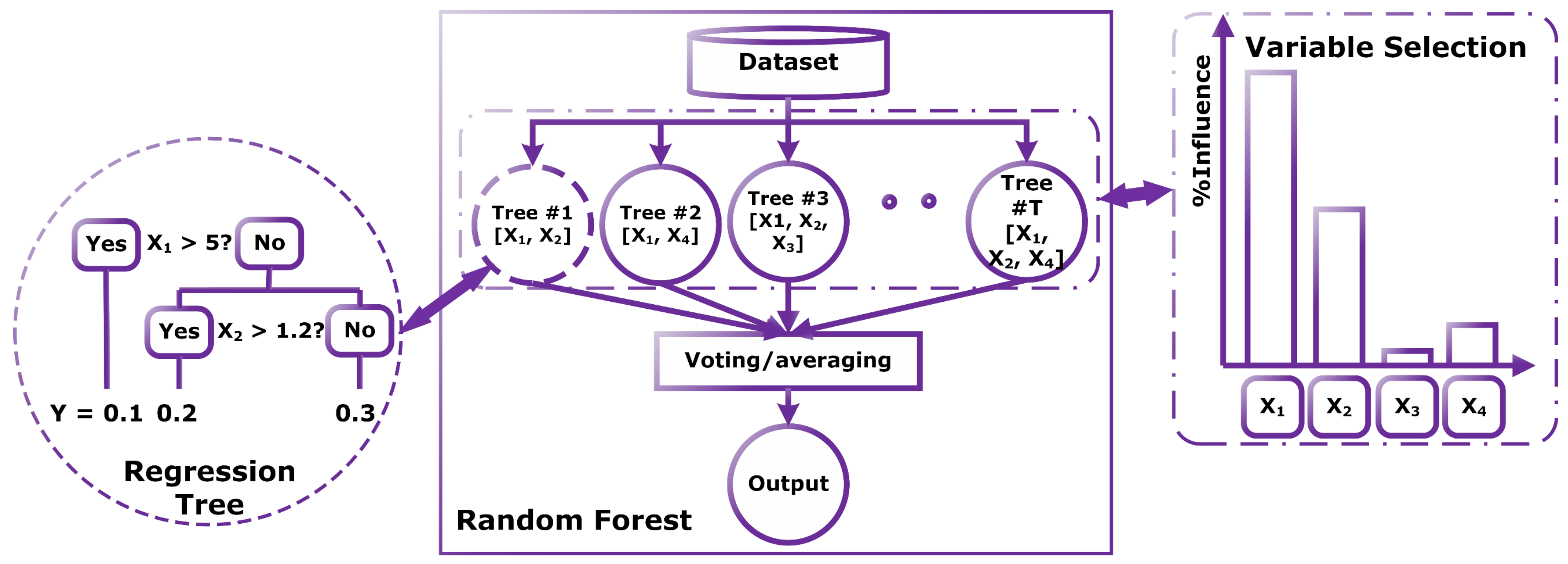
Table 1, random forest (RF) ensembles are known to be equally precise and stable in similar problems [28]. They have been used in scarce studies, as demonstrated in Table 2. It should be noted that the studies summarized in this table have several significant differences other than what is stated in the table, such as the approach and frequency of collecting the data, and the techniques for model development and construction.
Based on this survey of the public literature, it can be stated that:
  • There is an apparent lack of studies on data-driven models of on-road vehicle emissions rather than emissions of engines running on testbeds due to the immense costs of required measurements, especially in urban areas of developing countries.
  • For Egypt, such studies are completely lacking, where classic models are used instead, which deviate significantly from real-world driving conditions [3].
  • The limited available models of on-road ERs are typically developed based on measurements carried out for specific vehicles or a limited fleet of vehicles, such as in [20], which limits their extrapolation potential to other vehicles in use in the same area.
  • Furthermore, these studies are mostly adopting ANN-based models for this purpose, which are known to be prone to overfitting and lack accuracy when carelessly developed.
  • The RF technique has been employed in [20] for one vehicle, but its potential in handling large datasets for a diverse fleet of vehicles is still to be addressed.
  • Vehicle category-based models seem to be a good compromise between vehicle-specific models and region-specific models in terms of accuracy and ability to generalize. RF excels in accepting both numerical and categorical inputs while having unbiased estimates. Yet, this has not been explored in the context of the present study to the best of the authors’ knowledge.
Motivated by the aforementioned research gap, the potential of the RF ensemble technique in estimating FC and on-road emissions of different categories of passenger vehicles is investigated in this study. The novelty and contributions of the study can be summarized as follows:
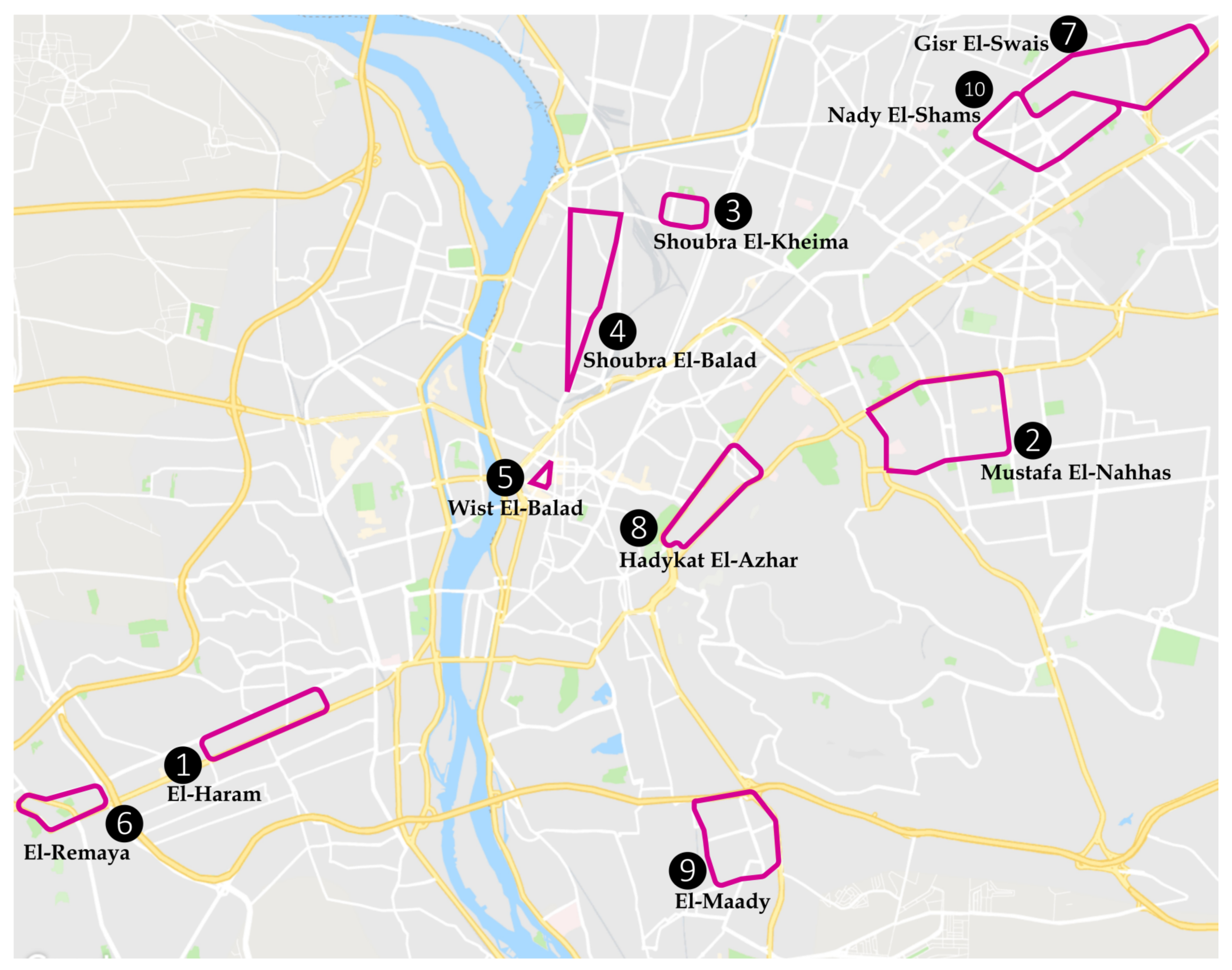
  • Five ensemble models are developed and validated carefully to estimate FC and emission rates (CO, CO2, NOx, and HC) for lightweight gasoline passenger cars in the metropolitan region of Greater Cairo, Egypt.
  • The models are developed based on extensive and precise onboard measurements from 87 vehicles driven over 10 different types of routes in the region.
  • The proposed models accept both numerical and categorical inputs, and the relative impact of each input variable is demonstrated to examine the potential of simplifying the models or testing their performance in case of incomplete data.
  • The models are also tested to evaluate their performances in terms of the dataset size (e.g., in the case of limited collected data) and the number of sub-decision trees (to evaluate the model robustness).
  • Finally, category-specific models were customized to check the possibility of increasing prediction accuracy when focusing on specific vehicle weight, age, and engine type combinations.
Therefore, the developed models can be viewed as sort of general models (in terms of vehicle specifications), customized for the specific characteristics of the study location, or other locations with similar traffic conditions, rather than for specific vehicles. The proposed algorithm is relatively simple and intuitive compared with other data-driven algorithms (such as ANNs), and can be adopted by interested researchers and engineers without deep expertise in machine learning. Such models not only would serve as a valuable tool in estimating the consumed energy and emitted pollutants in the transportation sector but can also help policymakers in planning a more sustainable urban transportation sector.

2. Materials and Methods

2.1. Study Area

The study takes place in Greater Cairo (GC), which is a highly urbanized and densely populated megacity, comprising multiple main cities in Egypt, such as Cairo, Giza, 6th of October, and El-Qalyubiyya. Egypt is known as the largest Middle Eastern country with a population of more than 100 million citizens and an annual increase in the population of around 2.7%. Vehicle ownership comes at a rate of ~0.12 cars per capita. More than 11.0 million vehicles are in use, and this number is increasing yearly at a rate of ~10%. There are 51, 1, and 14% light-weight vehicles, city buses, and heavyweight vehicles among these vehicles. The rest of the vehicles are motorcycles and other special-use vehicles [31].
Being an urban area in a developing country and one of the oldest and most populated areas worldwide, the driving patterns and conditions in GC can be expected to significantly deviate from those of developed countries. Specifically, the roads in GC are relatively narrow, especially in residential areas. Over time, the road network has been expanding to accommodate the increasing population, with heterogeneous traffic comprising vehicles of different sizes and purposes, ranging from motorcycles to city buses. With the lack of reliable automated traffic management systems in most streets, the driving process is primarily non-lane-based, with generally slower vehicle speeds and higher ERs [3,31]. Traffic congestion can be particularly noticed in small arterials in low-income areas, where the street is partially used for parking and marketing. In the same areas, there is a lack of traffic lights and strictly identified pedestrian crossings, which results in aggressive driving and frequent accelerations and decelerations with the semi-random crossing behaviors of pedestrians. Last but not least, the Egyptian vehicular standards, despite being frequently updated, are still falling behind those of the US or EU, where even vehicles manufactured in the past century are still in use, resulting in higher ERs in the city [3,31].
The aforementioned key differences between the traffic conditions and road networks in GC as a developing metropolitan area and similar urban areas in developed countries make it challenging to accurately develop reliable models for the prediction of FC and ERs of vehicles. The models described in the following sections can be re-developed for other regions worldwide, and they are expected to provide even more accurate estimates under more regulated and predictable traffic conditions.

2.2. Field Investigation and On-Road Measurements

To represent the driving patterns in different areas of GC in a cost-effective way, representative driving routes were identified by transportation experts as part of the “Sustainable Transport Project for Egypt” project, as detailed in [3]. These routes were selected based on different features, most notably the location, width, and the number of lanes of the street, the nominal traffic conditions, and the type and level of income of the surrounding areas. These routes are graphically shown in Figure 1. The 10 routes were, respectively, covered by 803, 69, 75, 94, 87, 80, 79, 73, 79, 83, and 84 trips by the vehicles described hereinafter, resulting in total distances of 4932, 203, 581, 506, 357, 121, 374, 1068, 860, 376, and 486 km. The reader is referred to [3] for more details on this route selection process.
Only gasoline passenger vehicles are considered in this study since the number of lightweight diesel vehicles is marginal in Egypt [32]. A field inventory followed by a technical check was carried out to identify the most frequently used vehicles in GC. A total of 87 cars were finally selected for the on-road measurements, as detailed in Table 3. The table shows 18 categories of these vehicles based on their production year, size, and fuel system. Each of the aforementioned routes was covered by at least 1 vehicle from each category in Table 3.
The on-road measurements of vehicular fuel consumption (FC) and ERs were carried out using the CATI’s OEM-2100AX® Axion unit [33,34], as shown in Figure 2. This unit measures the carbon emissions (CO2 in g/s, CO in mg/s, and HC in mg/s) via a non-dispersive infrared gas analyzer. Meanwhile, an electrochemical sensor is employed for measuring the NOx ER (in mg/s). Other measurements of the unit include the FC rate (g/s), intake air flow rate (g/s), intake pressure (kPa), intake temperature (IAT, °C), intake relative humidity (%), manifold pressure (MAP, kPa), and manifold temperature (°C). The unit uses the speed density method to determine the exhaust gas flow rate (g/s) [35]. The unit also recorded the car speed (km/h), engine speed (RPM), location (longitude in °N, latitude in °E, elevation in m above sea level, and local date and time using an integrated GPS unit). The category of the car (based on year, size, and fuel system) was manually recorded.
The measurements were performed on a 1.0 Hz basis during 106 weekdays (Sunday to Thursday in Egypt), distributed over 14 months of field activities based on the availability of the 87 vehicles (driven by their owners, rather than professionals). All measurements were carried out during working hours (6:00 to 18:00). The unit was carefully checked before any planned trip of each vehicle and was calibrated frequently, as detailed in [3] based on the 2-point method [34].

2.3. Data Processing

The two steps of data processing and model development were carried out in MATLAB R2020a. Data files of incomplete trips were entirely discarded in the later steps of the study. A considerable fraction of the raw dataset was excluded based on the detected anomalies or faulty data records (e.g., negative values), especially in the measured ERs due to drifts in the sensors or errors in the unit’s setup. The data files were checked after each trip to decide whether a calibration process was required. The final processed dataset, used for training and testing the RF models, comprised a total of 803 round trips for a total distance of ~4932 km over a total of ~255.56 h of driving.

2.4. Model Development and Evaluation

2.4.1. Decision Tree Regressor

The RF algorithm is an extension of the regression tree (RT) concept. Regression trees, which were originally proposed by Breiman et al. [36], are simple, non-parametric methods that apply the concept of recursive-partitioning regression, where the input space is split into many smaller regions and the estimated output of each region is simply the average of all observations falling in that region [37]. Starting with a single first decision (root), the RT is grown to some terminal nodes, where the final decision is made, as illustrated in Figure 3. Some decision nodes determine the outcome based on a splitting criterion between the root and the terminal leaves. Typically, the split is made at the point that maximizes the reduction in prediction error. For instance, at node t of an RT (T), the objective is to determine the optimal split s t for which splitting the input N t samples into the left and right branches ( t L and t R ) maximizes the drop Δ E s , t of an impurity/error measure E t :
Δ E s , t = E t p L E t L p R E t R
where
p L = N t L / N t
p R = N t R / N t
RTs are grown until a predetermined number of observations at the terminal nodes is obtained [38]. Detailed computations of RT regressors are provided in [39].
Figure 3. A schematic of the training and variable selection processes in the RF algorithm.
Sustainability 15 01503 g003

2.4.2. Random Forest Ensemble

RTs are relatively weak and unstable learners. Fortunately, they can be used as base learners in more powerful ensembles, such as the RF regressor [28]. In RF, many bootstrap samples are drawn from the original dataset, and each sample is used to fully grow an RT, as shown in Figure 3. The input variables selected at each decision node are randomly selected to reduce the correlations between the different grown RTs. Eventually, each RT is used to estimate the desired output, and the final prediction of RF is simply the average of all RTs predictions (aggregation step) [36,38,39].
In RT-based ensembles, the bagging concept is the concept of aggregating the predictions of different weak sub-learners to come up with a strong global learner. For a training dataset G = X i , Y i ,   i = 1 ,   ,   n , a B number of samples (bootstrap samples) is extracted from the global dataset, where each bootstrap has the same distribution as the original dataset. Then, these samples can be expressed as G * b = X i * b , Y i * b , and each bootstrap ( G * b ) is used to grow a different RT ( T * b ) to build a new sub-learner μ ^ * b X . Therefore, the final estimation of the ensemble is simply the arithmetic average of the estimates offered by all RTs, i.e., [36,38,39]:
μ ^ b a g X = 1 B b = 1 B μ ^ * b X
Knowing that each RT is only trained by a subset of the data, the ensemble can be evaluated using out-of-bag (OOB) observations. For a specific RT, OOB data points are those excluded from the training dataset of that RT.
The RF algorithm extends the bagging concept by taking samples of the model inputs at each node to make the optimal split (alongside taking samples of the training data). This is to increase the diversity and decrease the inter-correlation of different grown RTs. Hence, the steps of the algorithm can be briefed as shown below [36,38,39].
  • Consider a global training dataset G = X i , Y i , with P representing the number of model inputs, m standing for the number of model inputs used in each node (i.e., m < P), and B standing for the number of bootstrap samples.
  • Repeat the following steps for b = 1, …, B:
    • Take a bootstrap sample ( G * b ) without replacement from G , with a size n.
    • Pick m input variables from the total set of P of the model.
    • Use the bootstrapped data and the selected m variables to make the best split.
    • Gradually grow the RT ( T * b ) by making successive splits until one of the stopping criteria is satisfied.
    • Create an independent random vector ( θ b ) for T * b , where the RT would be defined as h X , θ b .
  • Feed the new input data X’ to all grown RTs so each can make a different estimate of the predicted variable.
  • Take the arithmetic average of the estimates offered by all RTs, as per Equation (5), which would be the final estimation of the RF model [36,38,39].
Y ^ X = 1 B b = 1 B h X , θ b
Aside from using it as a predictive least-square-based algorithm for estimating the emission factors, RF is also used for assessing the relative importance of input variables (I), i.e., for determining the most influential input variables. According to Breiman [36], this is achieved by weighting the error drops p t   Δ E s t , t of all nodes t in which the variable X p is used as a splitting criterion, averaged over all RTs ( N T ) in the ensemble:
I X p = 1 N T T = 1 N T t T : v s t = X p p t   Δ E s t , t
where p t = N t / N , i.e., the proportion of data points reaching the t split, while v s t is the variable used for splitting the input space at the t node. Of course, this can be achieved using the RTs. However, due to the inherent instability of those learners, the estimated relative influences are more likely to change from a grown RT to another one trained using the same dataset [38,40].

2.4.3. Developed Model

Following the major objective of the study to develop global (independent of fuel type/engine model), yet local (dependent on specific driving patterns in developing cities) models of vehicle emissions, 4 models were developed for predicting the emission factors, namely carbon dioxide (CO2), carbon monoxide (CO), nitrogen oxides (NOx), and unburned hydrocarbons (HC), using the RF algorithm. Eight candidate inputs (model year, vehicle size, fuel system, vehicle speed, engine speed, VSP, FC, and engine stress) were selected to develop the models as shown in Table 4. The first 3 inputs are categorical and their values are based on the categories shown in Table 3. The model year or vehicle’s age value can be very old (before 1980), old (1981–1990), new (1991–2000), or very new (after 2000). The vehicle size value can be small, medium, or large. The fuel system value can be SPI, MPI, or CRB (see Table 3). Meanwhile, the remaining inputs are numerical and their descriptive statistics are provided in Table 4. All numerical inputs were measured except for the vehicle-specific power ( V S P in kW/ton) and the engine stress ( S t r e s s ), both determined here based on the EPA’s IVE model, as follows [41]:
V S P = 1.1   C   S + 0.132   S + 0.000302   S 3 + 9.81 tan 1 sin R G
S t r e s s = i R P M + 0.08   P A P
where S and C are the speed (m/s) and acceleration (m/s2) of the vehicle, respectively, R G is the road grade (radians), i R P M is the RPM index, and P A P is the pre-average power [3,41,42]. The fifth and last model of FC is developed using the same set of inputs, except for the second last one (FC).
It should be noted that these models aim to predict the rates (per unit time) at which the vehicles consume fuel or emit pollutants. Hence, FC and CO2 are predicted in g/s whereas CO, NOx, and HC are predicted in mg/s. Some studies in the literature present these rates per unit distance (e.g., g/km). Such an estimation can still be undertaken using the developed models via a simple conversion (as shown in [3] for example). Other studies estimate trip energy consumption (TEC), which is a more suitable unit for other types of vehicle, such as EVs [43], or city buses with fixed routes and schedules [44].
A 5th model has been developed using the same approach to predict the fuel consumption (FC) of the vehicle in g/s based on the 7 inputs in Table 5. In the 4 aforementioned ER models, FC is considered a known model input. However, if both FC and ERs are to be predicted simultaneously, the 5th model can be used first to estimate FC, and then, these estimates of FC can be used in the first 4 models to estimate CO2, CO, NOx, and HC. It should be noted that the models of the 5 variables (CO2, CO, NOx, HC, and FC) are developed separately. In other words, each model has a single output (CO2, CO, NOx, HC, or FC). The ER models accept the 8 inputs in Table 4, whereas the FC model accepts only the 7 inputs in Table 5.

2.4.4. Computations and Model Evaluation

After the data preprocessing step described in Section 2.3, a data reduction step was carried out for FC and ER modeling to reduce the computational costs of the data-driven algorithm and to eliminate the influence of potential outliers on the predictive accuracy of the developed models. The reduction was accomplished by averaging the 1.0 Hz sequential observations corresponding to the same driving mode, i.e., idling, cruise, acceleration, and deceleration. As shown in Table 4, this step considerably reduces the dataset size from 806,584 to 121,581 observations without significantly influencing the overall descriptive statistics of the models’ inputs and outputs.
The training process starts by identifying the appropriate inputs among the 8 candidate inputs discussed above. Next, the number of grown RTs and the maximum number of observations at tree terminal leaves are set to 500 RTs (the significance of this number will be discussed in Section 3.2) and 5 observations, respectively. The number of randomly selected inputs at each split is set to one-third of the number of model inputs [45]. The reduced dataset is then perturbed and split into 2 subsets for training and testing the models, with size fractions of 0.7 and 0.3, respectively. The models’ training was carried out using custom scripts, with the aid of the treebagger function in MATLAB R2020A®. Out-of-bag samples from the training subset are used routinely to adjust the tree parameters to minimize the cost function (mean squared error) and the training continues until the stopping criteria are met. Finally, the testing subset is used to evaluate the performance of the trained model in simulating new data that were not used in the training phase. The prediction accuracy is measured using 3 statistical indicators, namely: mean bias error (MBE), root mean squared error (RMSE), and coefficient of determination (R2) [46,47,48,49,50,51,52], all defined as follows:
M B E = n = 1 N O n ^ O n N
R M S E = n = 1 N O n ^ O n 2 N
R 2 = 1 n = 1 N O n ^ O n 2 n = 1 N O n O n ¯ 2
In Equations (9)–(11), the actual and estimated outputs of the model are, respectively, represented by O n and O n ^ , where n is the observation index ( 1 n N ), and the number of observations ( N ) is listed in Table 3. Meanwhile, O n ¯ is the average of measured values. Based on these equations, the model performs better as its M B E and R M S E measures approach 0.0, and its R 2 reaches to 1.0 [53].

3. Results and Discussion

As discussed previously, the RF algorithm is proposed for modeling emission factors in Greater Cairo. Compared with other data-driven algorithms, the relatively stable nature of the algorithm makes it a strong candidate for simulating highly stochastic datasets [28].

3.1. Overall Performance of the Models

At first, the five suggested models of FC and ERs (CO2, CO, NOx, and HC) were developed using the complete list of inputs (seven and eight candidate inputs for FC and ERs, respectively), with a model size of 500 RTs. The error values of the models are provided in Table 6, whereas goodness-of-fit plots of the models are shown in Figure 4. In this figure, the data points are distinguished by color based on whether they have been used for training or testing the models. The figure shows different predictive accuracies of the five models depending on the strength of correlations between the FC/ERs and the proposed inputs. The CO2 model shows excellent estimations with correlation coefficients of 0.989 and 0.972, corresponding to the training and testing datasets, accordingly. The corresponding MBEs are nearly zero in both stages, whereas the RMSEs are lower than 0.2 g/s. Based on the R2 values, the model manages to explain more than 97% of the variance in the two subsets. The close values of errors in the two phases suggest that the model can be used for efficient prediction of CO2 emissions at such a large scale without considerable overfitting.
Figure 5 further highlights the model’s accuracy by showing a series plot of 150 data points randomly selected (nonconsecutive) from the testing dataset. A very strong agreement between the observed CO2 ERs and the corresponding predictions can be noticed. The nearly normal distributions of the training and prediction errors, as displayed by the corresponding histogram, emphasize the proper training of the model as there are no significant patterns in the residuals (centered around a zero value).
The second model shows less accurate, yet very good, estimations of CO ERs. The test MBE and RMSE, respectively, are 0.666 and 94.871 mg/s. The model shows higher levels of unexplained variance in the measured dataset, with a testing R2 of 0.814. This can be noticed in the higher level of dispersion around the perfect model line (y = x). However, the corresponding series plot in Figure 5 still shows a strong agreement between measured and estimated values.
As for the NOx emissions, the developed model generally shows underestimations in the range of high ERs, as displayed by the deviation of the data points away from the reference line in Figure 4 and Figure 5 for NOx rates higher than 50 mg/s. For lower ERs, the data points are clustered around the reference line, but with a higher level of dispersion. Overall, the model explains more than 64% of the variance of the input data, which is satisfactory considering the high diversity in the used vehicles. On the other hand, the HC model seems less reliable for predicting the unburned hydrocarbons in the considered scale, or with the suggested inputs. It tends to overestimate the high HC rates. The test RMSE value is almost double that of the training phase, showing a tendency to overfit new data. Figure 5 highlights the lower potential of this model in simulating high HC data points, compared with the previous models. If the same model is fed with more homogenous data, e.g., data from a few specific types of vehicles (especially new cars), it is expected to have higher prediction accuracy. This is because the HC ER is less correlated to the adopted input engine variables, compared with, e.g., CO2, especially in relatively old vehicles. Finally, the FC model shows very good agreement with the observed data, showing a performance comparable to that of the CO model. Specifically, it explains more than 73% of the variance in the observed data, with a test RMSE of 0.214 g/s.
There are considerable differences between the models developed here and those offered in previous studies (as shown in Table 2) in terms of the studied region, types of model inputs, and dataset size and diversity. This does not allow for a fair direct comparison. However, Table 6 shows that the dimensionless error levels reported here are competitive. For instance, Table 6 demonstrates a testing coefficient of determination (R2) of 73.5%, which is in the same order of magnitude as the one reported by Yang et al. [30], i.e., 77.6%. Massoud et al. [29] reported larger R2 (up to 89.6) values, but this is due to the lower resolution dataset they employed, making predictions relatively easier.

3.2. Impact of the Dataset Size and Number of RTs

The sensitivity of the developed models to the size of the dataset and the number of RTs is shown in Figure 6 based on a different set of model training. The R2 value in prediction is plotted against five values of ensemble size (50, 100, 200, 300, and 400 RTs) and five values of the data fraction, i.e., the number of used data points divided by the size of the reduced dataset (121,581 observations). The figure clearly shows that the models’ performances are mostly insensitive to the number of observations if they are sufficient and have the same characteristics as the original dataset (representative of the population), which should justify the prior decision to reduce the dataset size saving the computational costs. In this figure, the smallest considered fraction is 0.2, which corresponds to 24,316 data points. On the other hand, the prediction accuracy is highly dependent on the number of RTs, especially for CO, NOx, and HC models, previously shown to be less accurate than the FC and CO2 models. All models showed some degree of improvement in the prediction accuracy as the number of RTs increased, until the number of trees came close to 500 trees, or even lower as in the case of the FC and HC models, where no more significant increase is obtained. Model sizes up to 1000 RTs were tried to make sure the developed models are not undertrained.

3.3. Relative Importance of Model Inputs

One of the merits of the RF algorithm is that it can be used to generate unbiased estimates of the relative influences of all candidate inputs on the models’ output, as discussed in Section 2.4.2. The relative influences of the suggested inputs of the FC and ER models are illustrated in Figure 7. The figure shows that for CO2 emissions, the most influential input is FC with a relative importance of ~48%, followed by the type of the fuel injection system ( S y s t e m ), which has considerably less influence compared to FC (~12% importance). As for the CO emissions, FC, vehicle size, and engine speed are the top inputs, with total relative influences of 59%. For the NOx emissions, FC is still the most influential factor (~25%), followed by the model year, the type of fuel injection system, and the engine speed (all ~15%). As for the HC emissions, the most influential variable is rather the VSP (~20%), followed by the model year, FC, and the type of injection system. The results presented in this figure could be used as a guide in developing similar models when not all such measurements are available.
Figure 8 is provided to demonstrate the anticipated level of prediction accuracy when only some of these inputs are used. To do so, eight models were trained and tested for each emission factor and seven models were developed for FC. The number of inputs of the eight models is increased from one to eight/seven. The first model of each emission factor is based on the most influential input, as shown in Figure 7, and for each of the following models, the next most important input is considered. As Figure 8 suggests, the prediction accuracy increases, and the prediction errors decrease as the number of inputs increases. This should be expected since machine learning models are generally greedy for high-dimensional input data. However, the accuracy of the ER models tends to stall at seven inputs, meaning that the engine stress can be safely removed from the list of input parameters without jeopardizing the models’ performances. The increase in training and prediction errors of most models with two or three inputs is attributed to the addition of categorical variables, whose values are not as diverse as those of numerical variables. Hence, it is recommended to consider categorical inputs only when at least three other continuous inputs are available.

3.4. Prediction Accuracy for Different Vehicle Categories

As discussed before, the prediction accuracy of the developed models is not expected to be as high as those of models developed for specific combinations of engine and fuel types using measurements made in the laboratory environment. The only exception was the CO2 model, which was superior due to the high correlation between FC/ERs and the selected inputs. This issue is further addressed in Figure 9, which shows the prediction errors of 18 category-based models, compared to those of the previously discussed models of all categories. These are the same categories shown in Table 3. In these models, the first three categorical inputs (model year, vehicle size, and type of fuel system) were omitted since they have the same value in the training and testing datasets of each model, and each ER model has been developed using the other five (numerical) inputs ( S p e e d , R P M , V S P , F C , S t r e s s ). Meanwhile, the FC model was developed using S p e e d , R P M , V S P , and S t r e s s as inputs. For these models, the original dataset has been used instead of the reduced dataset because some categories have limited numbers of data points in the reduced dataset, such as the 8th category (see Table 3). By inspecting Figure 9, it can be noticed that the accuracy of the developed models is highly dependent on the characteristics of the vehicles. The MBEs can be higher or lower than those of the all-data models, which is the reason behind the relatively marginal MBEs of the all-data models (i.e., positive and negative MBEs of different vehicles nearly cancel each other). The same applies to the RMSEs. However, a potential for substantially reducing the random error components by focusing on specific vehicle categories can be noticed in the figure, where RMSEs can be reduced by up to 69.7, 85.9, 77.9, 97.8, and 61.6%. It should be noted that this potential exists for specific vehicle categories, let alone specific vehicle models. The figure also shows that, in general, the emissions from very new cars, especially the small ones (e.g., category #1), are more predictable than the emissions of other categories.

3.5. Comparison with ANN models

To further demonstrate the reliability of the proposed RF models, they were compared with ANN models using the same training dataset. ANNs are employed as reference algorithms since they are by far the most commonly used algorithms for such a purpose in the literature. Specifically, five ANN models were developed for each car category to estimate CO2, CO, NOx, HC, and FC, similar to that undertaken in Section 3.4 with RF models. The models are of the multi-layered feedforward backpropagation architecture, where the number of neurons and hidden layers have been optimized by trying up to 300 neurons and three layers to minimize the validation errors. Then the models were tested independently to evaluate their generalization abilities. All models comprise tangential sigmoid and simple linear activation functions in the hidden and output layers, respectively, and were trained using the Levenberg–Marquardt learning algorithm. Since the models of the five predicted variables (CO2, CO, NOx, HC, and FC) are developed separately, the output layer of each model had a single neuron only. Size fractions of 0.7, 0.15, and 0.15 were used to split the dataset of each vehicle category (see Table 3) into three subsets for training, validation, and independent testing of the models. In addition, the following hyperparameters were also employed since they are commonly used in similar problems [54]:
Maximum number of training epochs/iterations = 1000 epochs.
Performance goal = 0.
Minimum gradient = 10−7.
Initial value of the control parameter ( μ ) = 0.001
Decrement and increment factors of μ are 0.1 and 10, respectively.
Based on the structural optimization of the ANN models, it was found that all models perform better and in a more stable manner with two layers only, i.e., a hidden layer and a single-neuron output layer. This can be ascribed to two factors: (1) the relatively limited dataset size for most of the categories presented in Table 3, and (2) the higher tendency of more complex models with multiple hidden layers to overfit when handling new observations. Hence, simpler two-layer models showed better stability with close magnitudes of errors in the training, validation, and testing phases. Table A1 depicts the best numbers of hidden neurons for the models developed for categories 1–18, respectively.
Figure 10 demonstrates the distribution of MBE and RMSE values for different car categories when using ANN models. It can be noticed that the bias errors and some of the random error components (represented by MBE and RMSE, respectively) are higher than those of RF models in Figure 9 despite optimizing the structure of ANN models and their better training error metrics. This is an intrinsic feature of ANN algorithms, comparedwith the more stable RF algorithm, as mentioned in Table 1. Figure 10 shows average MBEs of −0.0011 g/s, 0.1281 mg/s, 0.0315 mg/s, 0.2562 mg/s, and 6.73 × 10⁻⁴ g/s for CO2, CO, NOx, HC, and FC, respectively. These errors are higher than those of RF models by 47.57, 38.92, 236.6, 14.86, and 203%, respectively. The average RMSEs of ANN models are quite similar to those of RF models, but the ANN models better estimate HC emissions with a lower average RMSE by 3.7%. This is a relatively small margin, compared with the drastic superiority of RF models in terms of bias errors, despite their intuitiveness and simplicity. Moreover, the ANN models show frequent failures in delivering decent accuracy with older and larger vehicles, which dominate the local market in Cairo. Finally, the RF ensembles have the additional merit of being able to accept categorical and numerical sets of inputs without being biased towards inputs with wider ranges.
Finally, it should be noted that such fast-prediction and accurate models of vehicles’ emission rates and fuel consumption could be utilized for different purposes, such as the estimation of the contribution of the transportation sector to global air pollution rates in the region, the certification procedures of vehicles before entering the market, and the advancement of vehicle telematics [55]. Classic telematics data are often collected from on-road vehicles to optimize and make recommendations for the best vehicle route, which could be the fastest, safest, shortest, or straightest route. Data-driven models, such as those developed here, enable more advanced optimizations to also select the routes with the lowest predicted fuel consumption and environmental footprint.

4. Conclusions

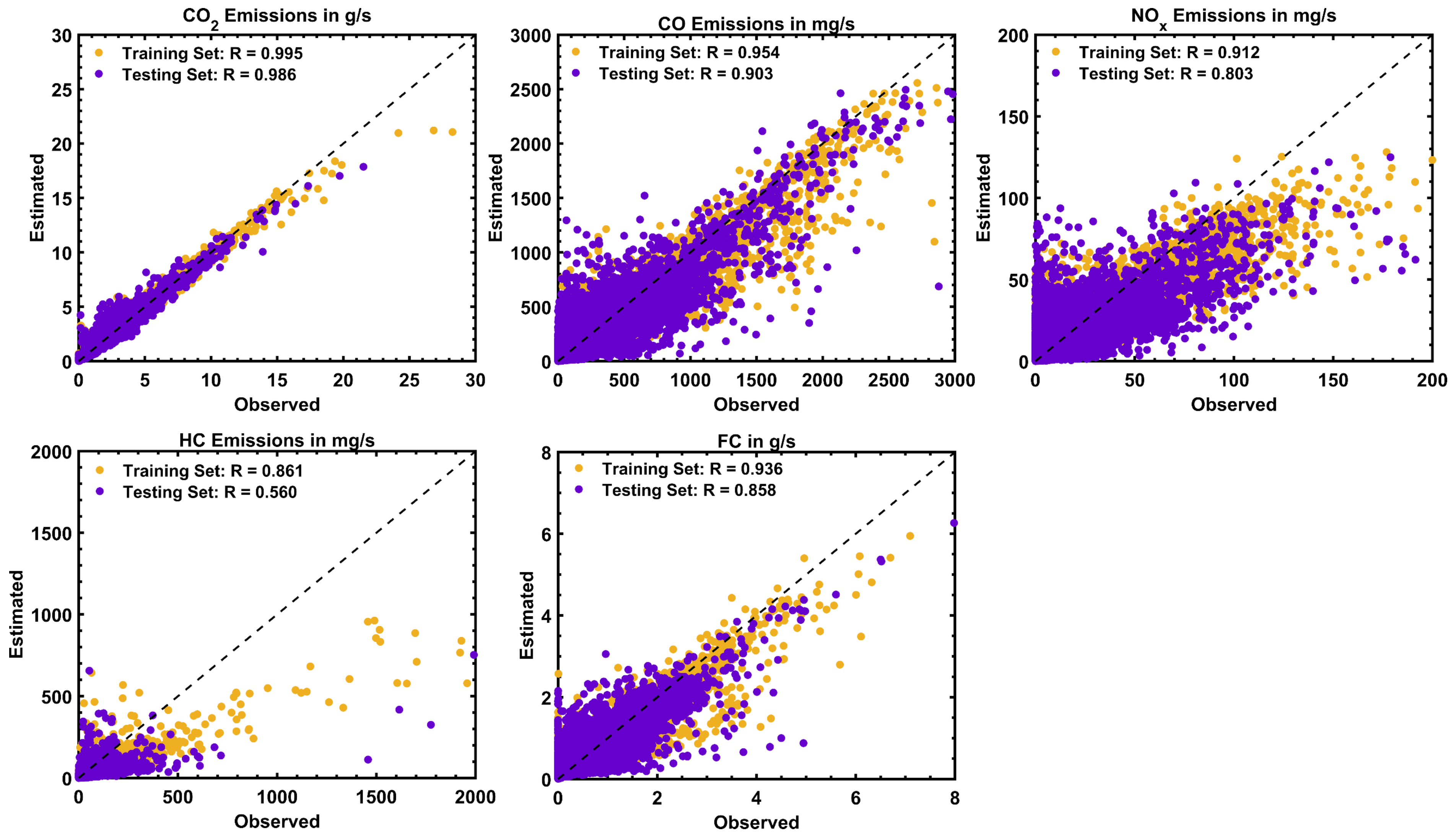
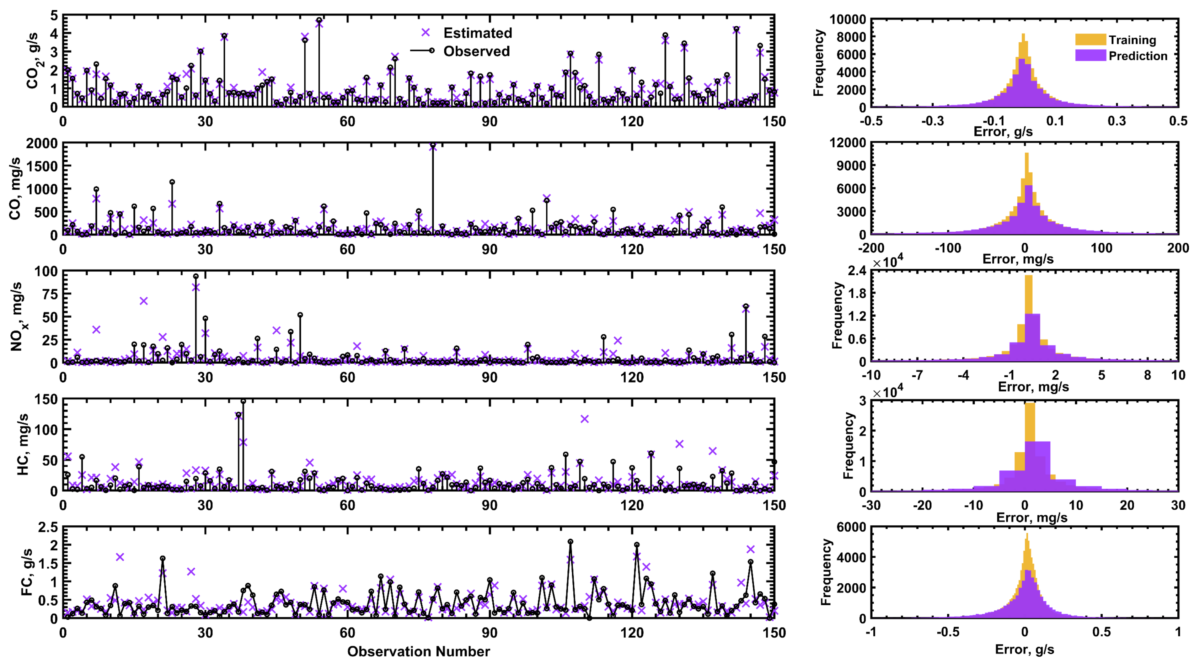
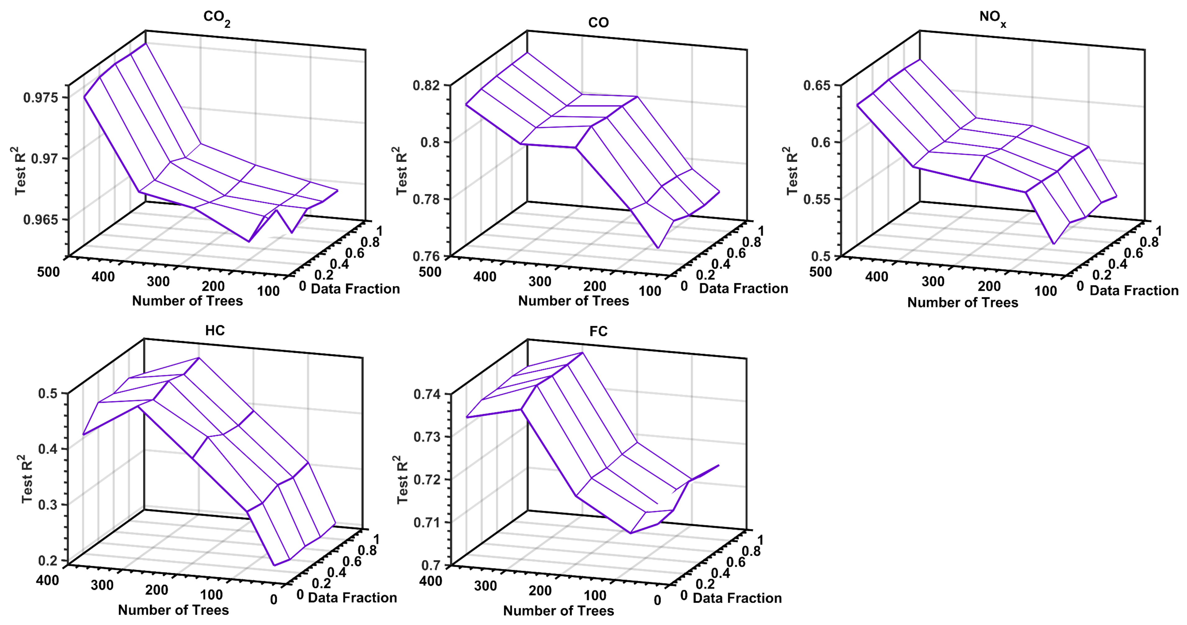
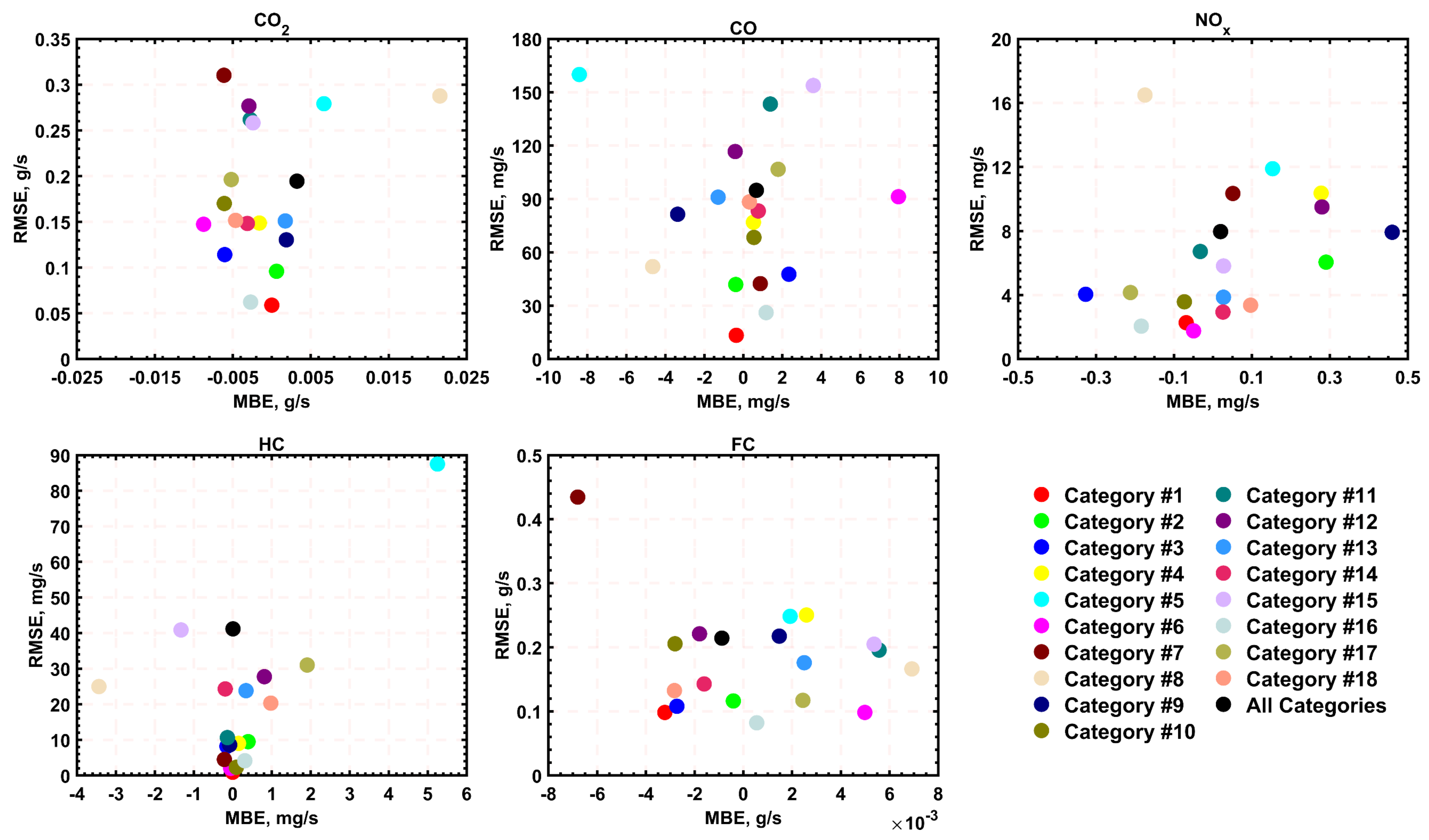
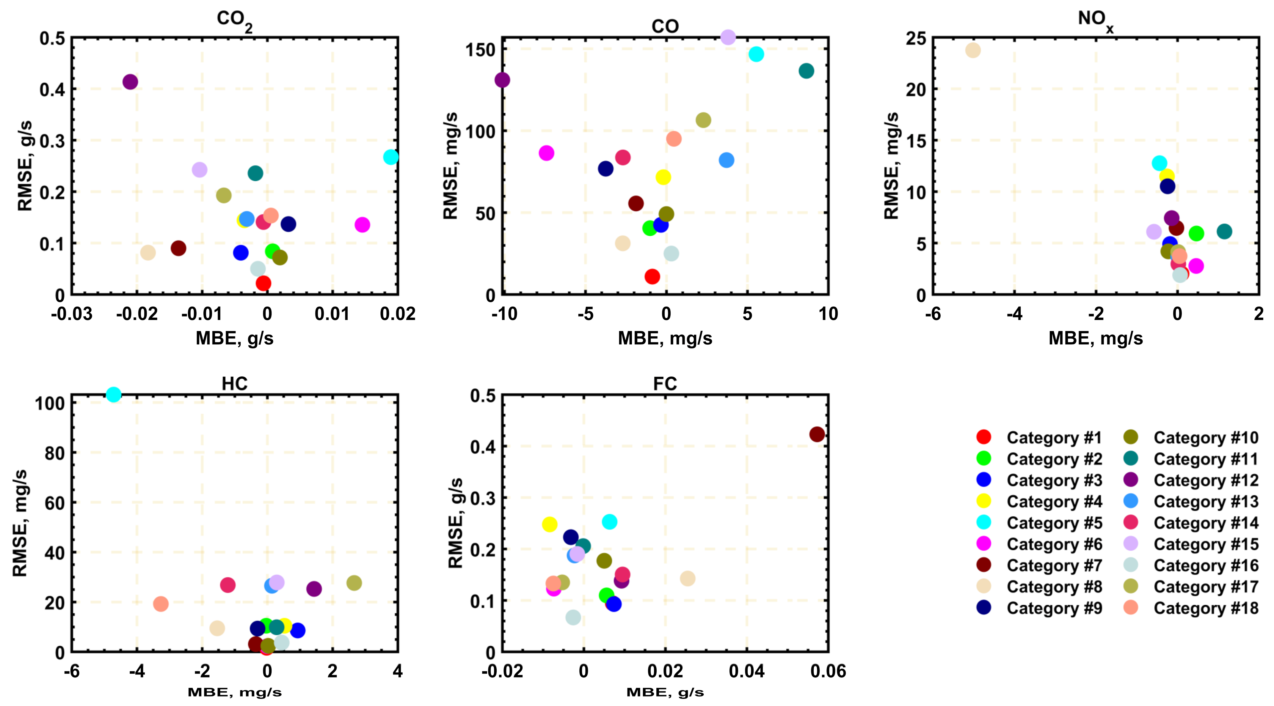
Models for predicting fuel consumption and onboard emission factors of conventional vehicles under real driving and traffic conditions are essential tools for various research and regulatory applications. The objective of this work was to develop the first set of such models for Greater Cairo, Egypt, based on extensive measurements using representative gasoline passenger vehicles and driving routes in the city. Five random forest regressor-based ensemble models were developed to be used for the various models of vehicles in the city. The results showed that RF models are most successful in predicting CO2 emission rates, where they explained more than 97% of the variance in the testing dataset. This was followed by the CO, fuel consumption, and NOx models, all providing satisfactory prediction accuracies. However, the HC model was the least reliable due to the diversity of considered vehicle models and the smaller correlation with input engine variables. It was also found that the prediction performance of those models is less sensitive to the size of the dataset, provided that it is sufficiently large, but considerably dependent on the RF ensemble size (up to 500 regression trees).
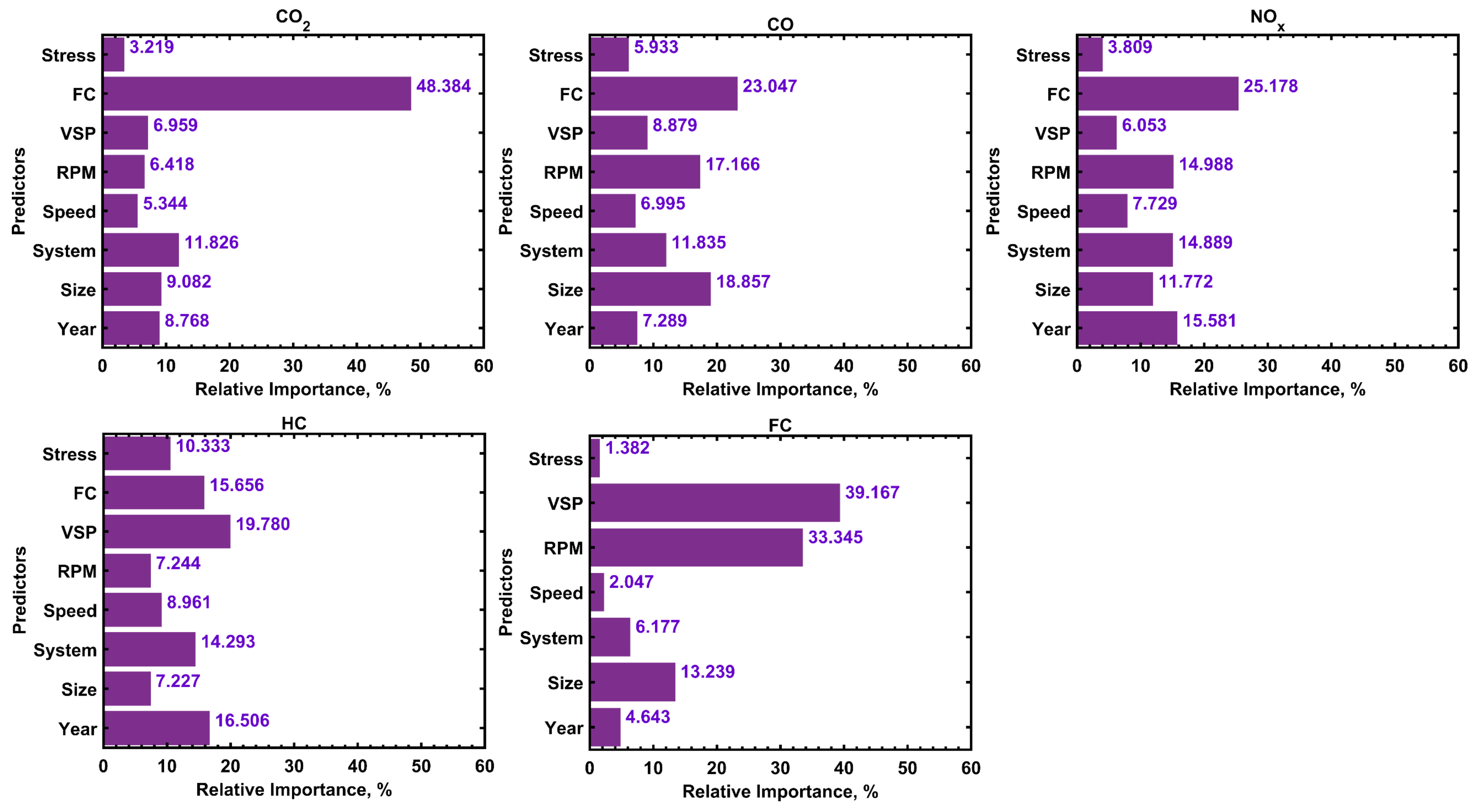
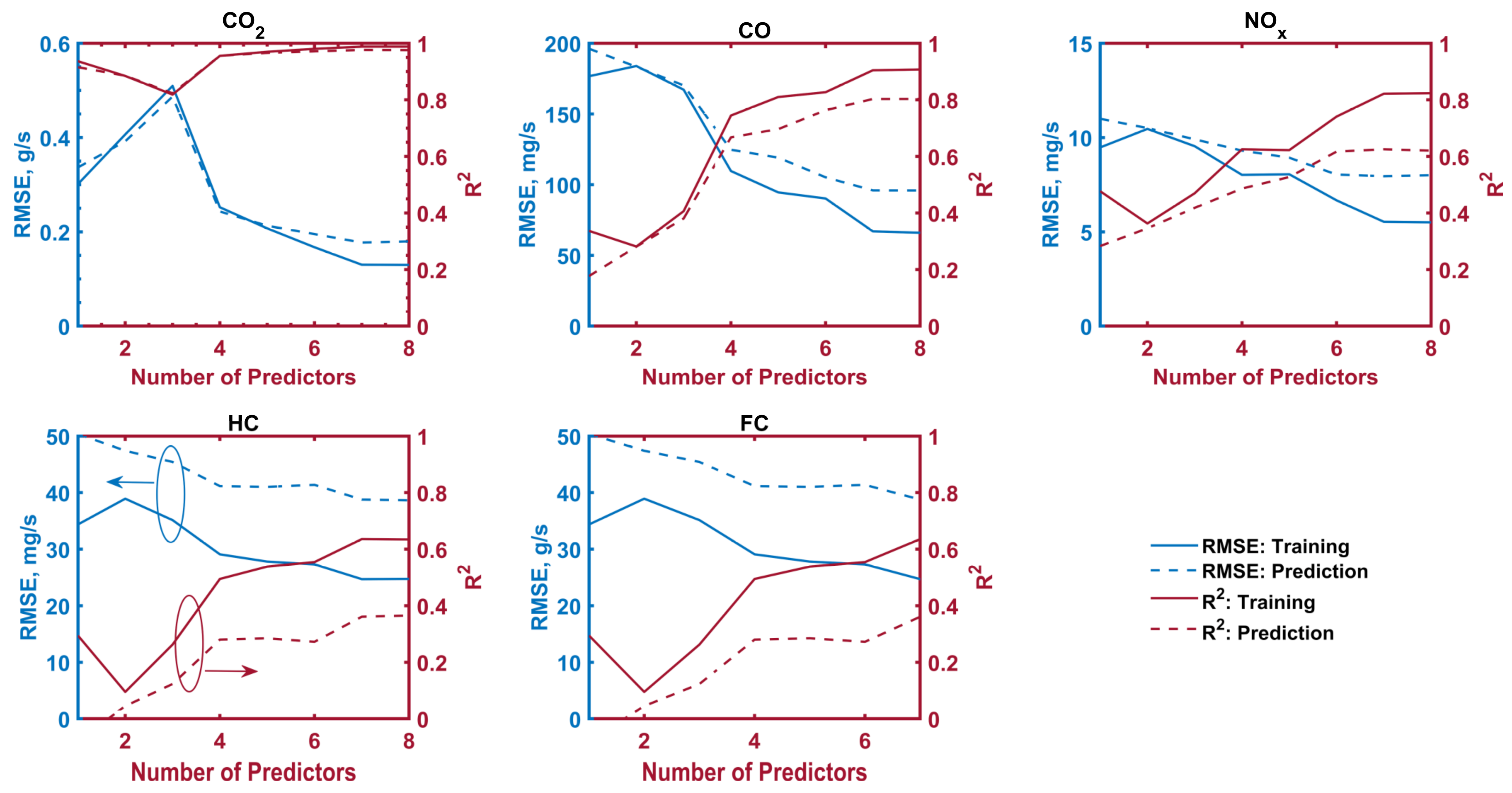
The relative importance of different model inputs has been highlighted for future studies on similar models, where it has been shown that fuel consumption is the most influential input (relative importance of >23%) for CO2, CO, and NOx predictions, followed by the engine speed and the vehicle category. The least influential input was the engine stress (<6%), which can be eliminated while having the same accuracy level. Finally, it has been shown that the accuracy levels of the different models can be boosted by limiting the dataset to specific vehicle categories, where the RMSEs can be reduced by up to 69.7, 85.9, 77.9, 97.8, and 61.6%, compared to the initially developed models of all vehicles.
For future works, specific engine/fuel-based models will be investigated using more complex techniques and additional explanatory variables to enhance the prediction accuracy of emission models. The RF models will be hybridized with optimization algorithms to ensure better stability. Finally, the performance of the models will be analyzed as a function of the traffic conditions, making it possible to develop hyper ensembles comprising sub-models for distinctive traffic conditions.

Author Contributions

Conceptualization, M.A.H. and H.S.; methodology and software validation M.A.H.; formal analysis and writing—original draft, M.A.H., H.S. and N.B.; writing—review and editing, M.A.H., N.B. and O.K.; All authors have read and agreed to the published version of the manuscript.

Funding

The authors received no specific funding for this study. Scientific support is mentioned in the acknowledgment section.

Institutional Review Board Statement

Not applicable.

Informed Consent Statement

Not applicable.

Data Availability Statement

The authors confirm that the raw dataset is not publicly available due to confidentiality agreements. Any related queries or requests to obtain the raw data can be directed to the entities mentioned in the acknowledgment. The rest of the data supporting the reported findings are all available within the article.

Acknowledgments

The measurements reported in this article are part of the Sustainable Transport Project for Egypt, carried out by the Transportation Program: Development Research and Technological Planning Centre (TP-DRTPC) at Cairo University, and sponsored by Global Environment Facility (GEF) and UNDP Cairo. Our appreciation is extended to all TP-DRTPC experts who participated in the “Measuring Emission Factors of Cars and Taxies in Grater Cairo” component, coordinated by the Egyptian Ministry of the Environment. The authors would like to thank Omar A. Huzayyin (Cairo University) for his input to this study.

Conflicts of Interest

The authors declare that they have no conflict of interest to report regarding the present study.

Appendix A

Table A1. The number of hidden neurons in the category-based ANN models.
Category NumberPredicted Variable
CO2CONOxHCFC
14455898677
249919715182
317106108128119
480105107153125
5155431301167
61304591907
740314289129
812552412583
91161471842126
10421361026063
11102547428152
121077513350140
1384518115493
145177575415
15110165514230
161301451523545
17140768312362
18461425045122

References

  1. Yang, N.; Yang, L.; Xu, F.; Han, X.; Liu, B.; Zheng, N.; Li, Y.; Bai, Y.; Li, L.; Wang, J. Vehicle Emission Changes in China under Different Control Measures over Past Two Decades. Sustainability 2022, 14, 16367. [Google Scholar] [CrossRef]
  2. Le Cornec, C.M.A.; Molden, N.; van Reeuwijk, M.; Stettler, M.E.J. Modelling of Instantaneous Emissions from Diesel Vehicles with a Special Focus on NOx: Insights from Machine Learning Techniques. Sci. Total Environ. 2020, 737, 139625. [Google Scholar] [CrossRef]
  3. Huzayyin, O.A.; Salem, H.; Hassan, M.A. A Representative Urban Driving Cycle for Passenger Vehicles to Estimate Fuel Consumption and Emission Rates under Real-World Driving Conditions. Urban Clim. 2021, 36, 100810. [Google Scholar] [CrossRef]
  4. Gebisa, A.; Gebresenbet, G.; Gopal, R.; Nallamothu, R.B. A Neural Network and Principal Component Analysis Approach to Develop a Real-Time Driving Cycle in an Urban Environment: The Case of Addis Ababa, Ethiopia. Sustainability 2022, 14, 13772. [Google Scholar] [CrossRef]
  5. Seo, J.; Yun, B.; Park, J.; Park, J.; Shin, M.; Park, S. Prediction of Instantaneous Real-World Emissions from Diesel Light-Duty Vehicles Based on an Integrated Artificial Neural Network and Vehicle Dynamics Model. Sci. Total Environ. 2021, 786, 147359. [Google Scholar] [CrossRef]
  6. Smit, R.; Ntziachristos, L.; Boulter, P. Validation of Road Vehicle and Traffic Emission Models—A Review and Meta-Analysis. Atmos. Environ. 2010, 44, 2943–2953. [Google Scholar] [CrossRef]
  7. Kancharla, S.R.; Ramadurai, G. Incorporating Driving Cycle Based Fuel Consumption Estimation in Green Vehicle Routing Problems. Sustain. Cities Soc. 2018, 40, 214–221. [Google Scholar] [CrossRef]
  8. Mera, Z.; Fonseca, N.; López, J.M.; Casanova, J. Analysis of the High Instantaneous NOx Emissions from Euro 6 Diesel Passenger Cars under Real Driving Conditions. Appl. Energy 2019, 242, 1074–1089. [Google Scholar] [CrossRef]
  9. Wang, C.; Ye, Z.; Yu, Y.; Gong, W. Estimation of Bus Emission Models for Different Fuel Types of Buses under Real Conditions. Sci. Total Environ. 2018, 640–641, 965–972. [Google Scholar] [CrossRef] [PubMed]
  10. Rahimi molkdaragh, R.; Jafarmadar, S.; Khalilaria, S.; Soukht Saraee, H. Prediction of the Performance and Exhaust Emissions of a Compression Ignition Engine Using a Wavelet Neural Network with a Stochastic Gradient Algorithm. Energy 2018, 142, 1128–1138. [Google Scholar] [CrossRef]
  11. Soukht Saraee, H.; Taghavifar, H.; Jafarmadar, S. Experimental and Numerical Consideration of the Effect of CeO2 Nanoparticles on Diesel Engine Performance and Exhaust Emission with the Aid of Artificial Neural Network. Appl. Therm. Eng. 2017, 113, 663–672. [Google Scholar] [CrossRef]
  12. Domínguez-Sáez, A.; Rattá, G.A.; Barrios, C.C. Prediction of Exhaust Emission in Transient Conditions of a Diesel Engine Fueled with Animal Fat Using Artificial Neural Network and Symbolic Regression. Energy 2018, 149, 675–683. [Google Scholar] [CrossRef]
  13. Yao, Y.; Zhao, X.; Liu, C.; Rong, J.; Zhang, Y.; Dong, Z.; Su, Y.; Chen, F. Vehicle Fuel Consumption Prediction Method Based on Driving Behavior Data Collected from Smartphones. J. Adv. Transp. 2020, 2020, 9263605. [Google Scholar] [CrossRef]
  14. Prasada Rao, K.; Victor Babu, T.; Anuradha, G.; Appa Rao, B.V. IDI Diesel Engine Performance and Exhaust Emission Analysis Using Biodiesel with an Artificial Neural Network (ANN). Egypt. J. Pet. 2017, 26, 593–600. [Google Scholar] [CrossRef] [Green Version]
  15. Li, Q.; Qiao, F.; Yu, L. A Machine Learning Approach for Light-Duty Vehicle Idling Emission Estimation Based on Real Driving and Environmental Information. Environ. Pollut. Clim. Chang. 2017, 1, 1–7. [Google Scholar] [CrossRef]
  16. Mądziel, M.; Jaworski, A.; Kuszewski, H.; Woś, P.; Campisi, T.; Lew, K. The Development of CO2 Instantaneous Emission Model of Full Hybrid Vehicle with the Use of Machine Learning Techniques. Energies 2022, 15, 142. [Google Scholar] [CrossRef]
  17. Silitonga, A.S.; Masjuki, H.H.; Ong, H.C.; Sebayang, A.H.; Dharma, S.; Kusumo, F.; Siswantoro, J.; Milano, J.; Daud, K.; Mahlia, T.M.I.; et al. Evaluation of the Engine Performance and Exhaust Emissions of Biodiesel-Bioethanol-Diesel Blends Using Kernel-Based Extreme Learning Machine. Energy 2018, 159, 1075–1087. [Google Scholar] [CrossRef]
  18. Wen, H.T.; Lu, J.H.; Jhang, D.S. Features Importance Analysis of Diesel Vehicles’ NOx and CO2 Emission Predictions in Real Road Driving Based on Gradient Boosting Regression Model. Int. J. Environ. Res. Public Health 2021, 18, 13044. [Google Scholar] [CrossRef]
  19. Chen, J.; Dobbie, G.; Koh, Y.S.; Somervell, E.; Olivares, G. Vehicle Emission Prediction Using Remote Sensing Data and Machine Learning Techniques. In Proceedings of the ACM Symposium on Applied Computing, Marrakech, Morocco, 3–7 April 2018; ACM: New York, NY, USA, 2017; pp. 444–451. [Google Scholar]
  20. Qiao, F.; Nabi, M.; Li, Q.; Yu, L. Estimating Light-Duty Vehicle Emission Factors Using Random Forest Regression Model with Pavement Roughness. Transp. Res. Rec. 2020, 2674, 37–52. [Google Scholar] [CrossRef]
  21. Gong, J.; Shang, J.; Li, L.; Zhang, C.; He, J.; Ma, J. A Comparative Study on Fuel Consumption Prediction Methods of Heavy-Duty Diesel Trucks Considering 21 Influencing Factors. Energies 2021, 14, 8106. [Google Scholar] [CrossRef]
  22. Bishop, J.D.K.; Molden, N.; Boies, A.M. Using Portable Emissions Measurement Systems (PEMS) to Derive More Accurate Estimates of Fuel Use and Nitrogen Oxides Emissions from Modern Euro 6 Passenger Cars under Real-World Driving Conditions. Appl. Energy 2019, 242, 942–973. [Google Scholar] [CrossRef]
  23. Ramos, A.; Muñoz, J.; Andrés, F.; Armas, O. NOx Emissions from Diesel Light Duty Vehicle Tested under NEDC and Real-Word Driving Conditions. Transp. Res. Part D Transp. Environ. 2018, 63, 37–48. [Google Scholar] [CrossRef]
  24. Jaikumar, R.; Shiva Nagendra, S.M.; Sivanandan, R. Modeling of Real Time Exhaust Emissions of Passenger Cars under Heterogeneous Traffic Conditions. Atmos. Pollut. Res. 2017, 8, 80–88. [Google Scholar] [CrossRef]
  25. Antanasijević, D.; Pocajt, V.; Perić-Grujić, A.; Ristić, M. Multiple-Input–Multiple-Output General Regression Neural Networks Model for the Simultaneous Estimation of Traffic-Related Air Pollutant Emissions. Atmos. Pollut. Res. 2018, 9, 388–397. [Google Scholar] [CrossRef]
  26. Azeez, O.; Pradhan, B.; Shafri, H. Vehicular CO Emission Prediction Using Support Vector Regression Model and GIS. Sustainability 2018, 10, 3434. [Google Scholar] [CrossRef] [Green Version]
  27. Moradi, E.; Miranda-moreno, L. A Mixed Ensemble Learning and Time-Series Methodology for Category-Specific Vehicular Energy and Emissions Modeling. Sustainability 2022, 14, 1900. [Google Scholar] [CrossRef]
  28. Hassan, M.A.; Khalil, A.; Kaseb, S.; Kassem, M.A. Exploring the Potential of Tree-Based Ensemble Methods in Solar Radiation Modeling. Appl. Energy 2017, 203, 897–916. [Google Scholar] [CrossRef]
  29. Massoud, R.; Bellotti, F.; Berta, R.; De Gloria, A.; Poslad, S. Exploring Fuzzy Logic and Random Forest for Car Drivers’ Fuel Consumption Estimation in IoT-Enabled Serious Games. In Proceedings of the 2019 IEEE 14th International Symposium on Autonomous Decentralized System (ISADS), Utrecht, The Netherlands, 8–10 April 2019. [Google Scholar] [CrossRef]
  30. Yang, Y.; Gong, N.; Xie, K.; Liu, Q. Predicting Gasoline Vehicle Fuel Consumption in Energy and Environmental Impact Based on Machine Learning and Multidimensional Big Data. Energies 2022, 15, 1602. [Google Scholar] [CrossRef]
  31. Timmermans, C.; Shawky, M.; Alhajyaseen, W.; Nakamura, H. Investigating the Attitudes of Egyptian Drivers toward Traffic Safety. IATSS Res. 2022, 46, 73–81. [Google Scholar] [CrossRef]
  32. El-Dorghamy, A.; Allam, H.; Al-Abyad, A.; Gasnier, M. Fuel Economy and CO2 Emissions of Light-Duty Vehicles in Egypt. Centre for Environment and Development in the Arab Region and Europe (CEDARE). Cairo, Egypt. 2014. Available online: www.globalfueleconomy.org (accessed on 1 December 2022).
  33. Wei, T.; Frey, H.C. Evaluation of the Precision and Accuracy of Cycle-Average Light Duty Gasoline Vehicles Tailpipe Emission Rates Predicted by Modal Models. Transp. Res. Rec. 2020, 2674, 566–584. [Google Scholar] [CrossRef]
  34. Khan, T.; Frey, H.C. Evaluation of Light-Duty Gasoline Vehicle Rated Fuel Economy Based on in-Use Measurements. Transp. Res. Rec. 2016, 2570, 21–29. [Google Scholar] [CrossRef]
  35. Sandhu, G.; Frey, H. Effects of Errors on Vehicle Emission Rates from Portable Emissions Measurement Systems. Transp. Res. Rec. 2013, 2340, 10–19. [Google Scholar] [CrossRef]
  36. Breiman, L. Random Forests. Mach. Learn. 2001, 45, 5–32. [Google Scholar] [CrossRef] [Green Version]
  37. Hassan, M.A.; Khalil, A.; Kaseb, S.; Kassem, M.A. Potential of Four Different Machine-Learning Algorithms in Modeling Daily Global Solar Radiation. Renew. Energy 2017, 111, 52–62. [Google Scholar] [CrossRef]
  38. Maindonald, J. Modern Multivariate Statistical Techniques: Regression, Classification and Manifold Learning, 1st ed.; Springer: Philadelphia, PA, USA, 2009; ISBN 9780387781884. [Google Scholar]
  39. Shanthamallu, U.S.; Spanias, A. Introduction to Machine Learning, 2nd ed.; The MIT Press: London, UK, 2022. [Google Scholar]
  40. Bai, Z.D.; Silverstein, J.W. Spectral Analysis of Large Dimensional Random Matrices, 1st ed.; Springer: London, UK, 1999; ISBN 9780387775005. [Google Scholar]
  41. Yao, Z.; Wei, H.; Liu, H.; Li, Z. Statistical Vehicle Specific Power Profiling for Urban Freeways. Procedia Soc. Behav. Sci. 2013, 96, 2927–2938. [Google Scholar] [CrossRef] [Green Version]
  42. Pouresmaeili, M.A.; Aghayan, I.; Taghizadeh, S.A. Development of Mashhad Driving Cycle for Passenger Car to Model Vehicle Exhaust Emissions Calibrated Using On-Board Measurements. Sustain. Cities Soc. 2018, 36, 12–20. [Google Scholar] [CrossRef]
  43. Liu, Y.; Zhang, Q.; Lyu, C.; Liu, Z. Modelling the Energy Consumption of Electric Vehicles under Uncertain and Small Data Conditions. Transp. Res. Part A Policy Pract. 2021, 154, 313–328. [Google Scholar] [CrossRef]
  44. Ji, J.; Bie, Y.; Zeng, Z.; Wang, L. Trip Energy Consumption Estimation for Electric Buses. Commun. Transp. Res. 2022, 2, 100069. [Google Scholar] [CrossRef]
  45. Oh, J.; Laubach, M.; Luczak, A. Estimating Neuronal Variable Importance with Random Forest. In Proceedings of the IEEE Annual Northeast Bioengineering Conference, Newark, NJ, USA, 22–23 March 2003; pp. 33–34. [Google Scholar]
  46. Bouchouicha, K.; Bailek, N.; Razagui, A.; EL-Shimy, M.; Bellaoui, M.; Bachari, N.E.I. Comparison of Artificial Intelligence and Empirical Models for Energy Production Estimation of 20 MWp Solar Photovoltaic Plant at the Saharan Medium of Algeria. Int. J. Energy Sect. Manag. 2021, 15, 119–138. [Google Scholar] [CrossRef]
  47. Elbeltagi, A.; Zerouali, B.; Bailek, N.; Bouchouicha, K.; Pande, C.; Santos, C.A.G.; Towfiqul Islam, A.R.M.; Al-Ansari, N.; El-kenawy, E.-S.M. Optimizing Hyperparameters of Deep Hybrid Learning for Rainfall Prediction: A Case Study of a Mediterranean Basin. Arab. J. Geosci. 2022, 15, 933. [Google Scholar] [CrossRef]
  48. Mustafa, J.; Husain, S.; Alqaed, S.; Khan, U.A.; Jamil, B. Performance of Two Variable Machine Learning Models to Forecast Monthly Mean Diffuse Solar Radiation across India under Various Climate Zones. Energies 2022, 15, 7851. [Google Scholar] [CrossRef]
  49. Jamei, M.; Bailek, N.; Bouchouicha, K.; Hassan, M.A.; Elbeltagi, A.; Kuriqi, A.; Al-Ansari, N.; Almorox, J.; El-kenawy, E.-S.M. Data-Driven Models for Predicting Solar Radiation in Semi-Arid Regions. Comput. Mater. Contin. 2023, 74, 1625–1640. [Google Scholar] [CrossRef]
  50. Yehia, M.H.; Hassan, M.A.; Abed, N.; Khalil, A.; Bailek, N. Combined Thermal Performance Enhancement of Parabolic Trough Collectors Using Alumina Nanoparticles and Internal Fins. Int. J. Eng. Res. Africa 2022, 62, 107–132. [Google Scholar] [CrossRef]
  51. Djaafari, A.; Ibrahim, A.; Bailek, N.; Bouchouicha, K.; Hassan, M.; Kuriqi, A.; Al-Ansari, N.; El-kenawy, E.-S. Hourly Predictions of Direct Normal Irradiation Using an Innovative Hybrid LSTM Model for Concentrating Solar Power Projects in Hyper-Arid Regions. Energy Rep. 2022, 8, 15548–15562. [Google Scholar] [CrossRef]
  52. Keshtegar, B.; Bouchouicha, K.; Bailek, N.; Hassan, M.A.; Kolahchi, R.; Despotovic, M. Solar Irradiance Short-Term Prediction under Meteorological Uncertainties: Survey Hybrid Artificial Intelligent Basis Music-Inspired Optimization Models. Eur. Phys. J. Plus 2022, 137, 362. [Google Scholar] [CrossRef]
  53. Hassan, M.A.; Khalil, A.; Abubakr, M. Selection Methodology of Representative Meteorological Days for Assessment of Renewable Energy Systems. Renew. Energy 2021, 177, 34–51. [Google Scholar] [CrossRef]
  54. MathWorks Deep Learning Toolbox. Available online: https://fr.mathworks.com/help/deeplearning/index.html?s_tid=CRUX_lftnav (accessed on 8 January 2023).
  55. Ghaffarpasand, O.; Burke, M.; Osei, L.K.; Ursell, H.; Chapman, S.; Pope, F.D. Vehicle Telematics for Safer, Cleaner and More Sustainable Urban Transport: A Review. Sustainability 2022, 14, 16386. [Google Scholar] [CrossRef]
Figure 1. The examined routes, superimposed on the map of GC.
Sustainability 15 01503 g001
Figure 2. FC and ER measurements using OEM-2100AX unit.
Sustainability 15 01503 g002
Figure 4. Correlations between observed and estimated ERs. Orange and violet colors indicate the data points of the training and testing subsets of the data.
Sustainability 15 01503 g004
Figure 5. Left: series of 150 actual ER values against their corresponding predicted values. Right: histograms of training and predicting errors.
Sustainability 15 01503 g005
Figure 6. Sensitivity of ensemble models to the dataset size and the number of RTs.
Sustainability 15 01503 g006
Figure 7. Relative importance of considered predictors on fuel consumption and emission rates.
Sustainability 15 01503 g007
Figure 8. The variation of the prediction accuracy with the number of explanatory variables. Blue and red curves represent the RMSE and R2 metrics (left and right axes, respectively). The solid and dash lines represent the training and testing phases of the model, respectively.
Sustainability 15 01503 g008
Figure 9. Scatter plots of the test MBEs and RMSEs of category-based and all-data models of ERs and FC using RF ensembles.
Sustainability 15 01503 g009
Figure 10. Scatter plots of the test MBEs and RMSEs of category-based models of ERs and FC using ANN models.
Sustainability 15 01503 g010
Table 1. Comparison between the commonly used algorithms in the literature for the prediction of FC and ERs in vehicles.
AlgorithmAdvantagesLimitationsExample Studies
Artificial neural networks (ANN)
  • Suitable for complex non-linear problems
  • Widely employed in the literature
  • Successfully used for different problems
  • Likely to overfit
  • Requires large training datasets
  • Could converge to local minima
[2,9,13,14]
Support vector machines (SVM)
  • High prediction accuracy
  • Highly stable
  • More likely to converge into the global minimum
  • Better performance with limited-size datasets
  • Better generalization accuracy
  • Higher computational cost in optimizing hyperparameters
  • Needs kernel functions
[13,15,16]
Extreme learning machine (ELM)
  • High accuracy levels
  • Less tendency to converge into local minima
  • Could be less accurate than ANN in complex problems
[17]
Gradient boosting (GP)
  • Intuitive and simple algorithm
  • Less tendency to overfit
  • Needs extensive hyperparameter optimization
  • Less accurate with large datasets
[18]
Random forest (RF)
  • Easier hyperparameter tuning compared to GP
  • More stable
  • Accepts both numerical and categorical inputs
  • Slow training and predictions when using large numbers of decision trees
  • Less accurate than ANN and SVM
[13,19,20,21]
K-nearest neighbor (KNN)
  • Institutive and simple
  • No learning costs
  • Robust to outliers
  • Less suitable for large and complex datasets
  • Intense training costs for large datasets
  • Sensitive to irrelevant or inter-correlated inputs
[15]
Table 2. Summary of the studies in the literature on using RF techniques for predicting vehicles’ FC and ERs.
AuthorsPredicted VariablesModel InputsFleet of VehiclesLocationModel Accuracy
Qiao et al. [20]HC, CO, NOx, CO2, and FCSpeed, acceleration, VSP, and roughness of the road.One vehicleTexasRoot mean square error < 6.4%
Yao et al. [13]FCDriving data collected from phone application (idle time, speed, acceleration, deceleration, etc.).20 taxis (same vehicle type)BeijingMean absolute error < 10% (better than ANN and SVM)
Gong et al. [21]FC21 inputs, including truck specifications, weather, road features, and vehicle status.34 diesel trucksJinan, ChinaPrediction accuracy of 86.6% (better than ANN and decision trees)
Massoud et al. [29]FCVehicle speed, the rotational speed of the engine, and throttle position.Collected data from Envirocar database-Coefficients of determination up to 89.6% (better than fuzzy logic)
Yang et al. [30]FC64 inputs of location, vehicle specifications, driving conditions, and weather. Data were collected from a phone application.Gasoline vehiclesChinaMean absolute percentage error of 7.5% and coefficient of determination of 77.6% (better than the five other algorithms)
Table 3. Size of the collected dataset (following preprocessing) and distribution of data points over the 18 different vehicle categories.
CategoryYearSizeFuel System#Cars#Original Datapoints#Reduced Datapoints
1>2001SmallMPI221,7373396
2 SPI327,7303690
3 CRB318,6482985
4 MediumMPI21191,15328,666
5 SPI440,3186150
6 CRB111,2601689
7 LargeMPI329,9264403
81991–2000SmallSPI21168200
9 CRB979,75112,100
10 MediumSPI219,8023587
11 CRB541,5246729
12 LargeSPI110,2381484
131981–1990SmallCRB10104,27215,135
14 MediumCRB874,38410,622
15 LargeCRB455,7488591
16<1980SmallCRB217,1802198
17 MediumCRB328,8123913
18 LargeCRB432,9336061
Total 87806,584121,581
SPI: single-point injection; MPI: multiple-point injection; CRB: carburetor.
Table 4. A list of the inputs and outputs of the models developed for predicting ERs, alongside their statistics.
VariableUnitTypeOriginal DatasetReduced Dataset
MeanMedianSTDMeanMedianSTD
OutputsCO2g/sNumerical1.0710.6451.2751.0720.6921.185
COmg/sNumerical141.967.46230.0145.876.16216.7
NOxmg/sNumerical6.3551.13015.485.6951.27913.06
HCmg/sNumerical14.595.86040.4115.676.53043.33
InputsModel year-Categorical------
Vehicle size-Categorical------
Fuel system-Categorical------
Vehicle speedkm/hNumerical19.2714.1018.0816.7612.36716.22
Engine speedRPMNumerical1628.61439.7932.71633.41463.7855.7
VSPkW/tonNumerical0.8920.0005.8240.4190.0006.145
FCg/sNumerical0.4190.2700.4490.4220.2900.417
Engine stress-Numerical4.2752.7823.6763.7422.6593.214
Table 5. A list of the output and inputs of the model developed for predicting FC, alongside their statistics.
VariableUnitTypeOriginal DatasetReduced Dataset
MeanMedianSTDMeanMedianSTD
OutputFCg/sNumerical0.4190.2700.4490.4220.2900.417
InputsModel year-Categorical------
Vehicle size-Categorical------
Fuel system-Categorical------
Vehicle speedkm/hNumerical19.2714.1018.0816.7612.36716.22
Engine speedRPMNumerical1628.61439.7932.71633.41463.7855.7
VSPkW/tonNumerical0.8920.0005.8240.4190.0006.145
Engine stress-Numerical4.2752.7823.6763.7422.6593.214
Table 6. Error statistics of the five developed models. The mean bias error (MBE) and the root mean square error (RMSE) have the same unit as the model output, whereas the coefficient of determination (R2) is dimensionless.
ModelTraining ErrorsTest Errors
MBERMSER2MBERMSER2
CO20.0000.1260.9890.0030.1940.972
CO−0.03066.350.9050.66694.870.814
NOx0.0065.5860.8140.0207.9630.642
HC−0.00722.820.6830.00441.170.301
FC0.0000.1500.871−0.0010.2140.735
Disclaimer/Publisher’s Note: The statements, opinions and data contained in all publications are solely those of the individual author(s) and contributor(s) and not of MDPI and/or the editor(s). MDPI and/or the editor(s) disclaim responsibility for any injury to people or property resulting from any ideas, methods, instructions or products referred to in the content.

