Article

Converting Seasonal Measurements to Monthly Groundwater Levels through GRACE Data Fusion

1
Department of Earth and Space Science, Southern University of Science and Technology, Shenzhen 518055, China
2
Department of Geomatics, National Cheng Kung University, Tainan City 701401, Taiwan
3
Civil Infrastructure Engineering Department, Institut Teknologi Sepuluh Nopember, Surabaya 60111, Indonesia
*
Author to whom correspondence should be addressed.
Sustainability 2023, 15(10), 8295; https://doi.org/10.3390/su15108295
Submission received: 6 April 2023 / Revised: 1 May 2023 / Accepted: 16 May 2023 / Published: 19 May 2023

Abstract

:
Groundwater depletion occurs when the extraction exceeds its recharge and further impacts water resource management around the world, especially in developing countries. In India, most groundwater level observations are only available on a seasonal scale, i.e., January (late post-monsoon), May (pre-monsoon), August (monsoon), and November (early post-monsoon). The Gravity Recovery and Climate Experiment (GRACE) data are available to estimate the monthly variation in groundwater storage (GWS) by subtracting precipitation runoff, canopy water, soil moisture, and solid water (snow and ice) from the GLDAS model. Considering GRACE-based GWS data, the data fusion is further used to estimate monthly spatial maps of groundwater levels using time-varying spatial regression. Seasonal groundwater monitoring data are used in the training stage to identify spatial relations between groundwater level and GWS changes. Estimation of unknown groundwater levels through data fusion is accomplished by utilizing spatial coefficients that remain consistent with the nearest observed months. Monthly groundwater level maps show that the lowest groundwater level is 50 to 55 m below the earth’s surface in the state of Rajasthan. The accuracy of the estimated groundwater level is validated against observations, yielding an average RMSE of 2.37 m. The use of the GWS information enables identification of monthly spatial patterns of groundwater levels. The results will be employed to identify hotspots of groundwater depletion in India, facilitating efforts to mitigate the adverse effects of excessive groundwater extraction.

1. Introduction

Groundwater plays a critical role as a valuable water resource for various industrial, agricultural, and domestic activities across the globe, such as in arid regions lacking freshwater (North Africa and the Middle East) or the most-populated countries, such as China and India. Overexploitation of groundwater leads to a scarcity of water resources at the regional level and poses a significant threat to social and economic development and the overall ecosystem [1]. Over the last few decades, severe groundwater extractions, mostly for irrigation purposes, have dramatically dropped hydraulic head levels in different regions of the world; within those areas, some areas dropped down by up to a few hundred meters [2,3]. Groundwater depletion rates are very high in several regions. As a result, the recovery process is not feasible in the foreseeable future. Excessive extraction of groundwater leads to the decline of this precious resource, requiring more energy to pump water as the groundwater level continuously drops [4]. The extreme groundwater depletion will compress the subsurface, which will lead toward land subsidence, like in some extreme cases such as the San Joaquim Valley of California; indeed, the land subsidence could reach 16 cm/yr during the second half of the last century [5]. Land subsidence has a high probability of increasing the risk of flood in the affected areas, such as Bangkok, Thailand, [6] and Jakarta, Indonesia [7].
GRACE and its follow-up mission GRACE-FO have been providing monthly observations of changes in the earth’s gravity field, starting from April 2002 [8,9]. GRACE is a tool used to assess temporal variations in the earth’s gravity field at a monthly temporal scale. Such variations are associated with several processes that need to be accounted for to estimate monthly changes in terrestrial water storage (TWS). Spatial and temporal changes in a gravitational field can be attributed to the variations in the mass of the fluidic layers of the earth [10]. The TWS is the sum of all storage components of water at and under the earth’s surface. These TWS datasets have been used by multiple studies globally, either at a regional scale (continental scale) or local scale (basin scale) (e.g., [11,12,13,14,15]).
Monitoring long-term cyclical changes in groundwater storage is critical to the sustainable development of ecosystems because groundwater is an important part of the hydrological cycle on earth [1,16]. However, accurate quantifications of groundwater level and its spatial and temporal variability are challenging due to the lack of monitoring data [16]. Limited groundwater level in the long-term and dense measurements serve as quantitative indicators of local groundwater change, so that a high spatiotemporal resolution groundwater level cannot be acquired easily [4]. Groundwater level data can be reconstructed using machine learning methods based on simulation models and GRACE data [17]. Groundwater data are temporally sparse in developing countries. For example, groundwater levels are observed during January, May, August, and November in India. The spatiotemporal GRACE TWS data reflect consistent patterns with that of hydroclimatic variables. Previous studies [18] used data from the Global Land Data Assimilation System (GLDAS) land surface models and decompose the GRACE TWS data into surface water, soil moisture, snow and canopy water, and groundwater storage (GWS). These datasets provided us with critical information for monitoring changes in GWS and are highly related to groundwater level [19]. Moreover, multiple GRACE mascon products were integrated with GLDAS outputs to estimate and analyze spatio-temporal variations in GWS anomalies [20,21,22]. Scanlon et al. (2018) considered GRACE data and various global hydrological models including GLDAS to assess the impacts of climate and humans on water resources [23]. The previous study proposed a fusion method incorporating spatially and temporally varying relations of data [24]. This study will consider the data fusion based on in situ groundwater observation and GRACE-based GWS.
Groundwater level measurements in India are generally recorded four times a year. Thus, the process of estimating monthly groundwater levels is employed from the integration of seasonal groundwater monitoring wells and monthly GRACE data. We make the assumption that the spatial relationship between groundwater levels and GWS changes remains constant between the observed month and the nearest ones. Data fusion is employed to link the GRACE-based GWS and groundwater level using time-varying spatial regression. Eventually, the monthly spatial groundwater level is estimated from GRACE-based GWS changes while the nearest month coefficients are identified.

2. Materials and Methods
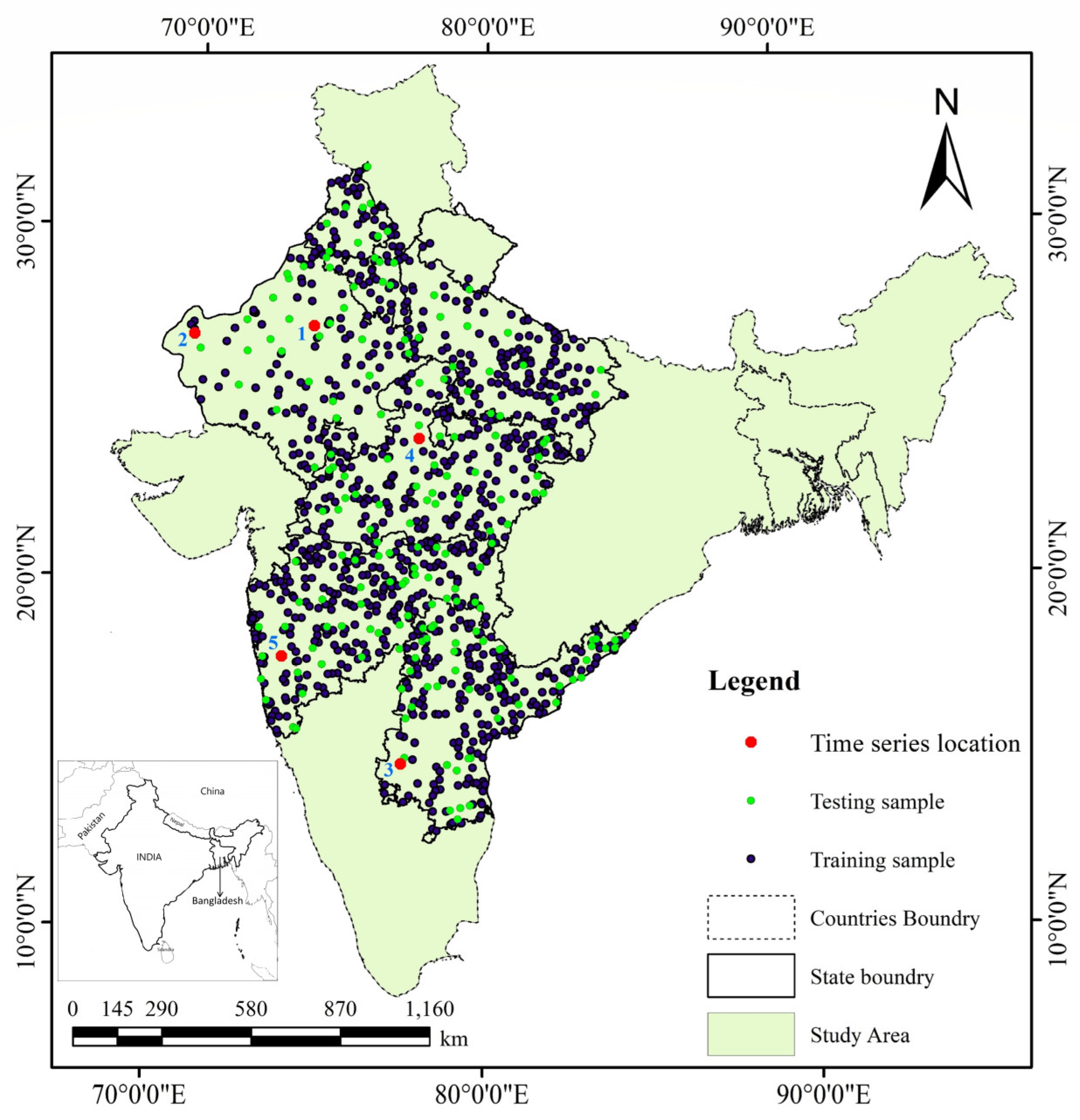
2.1. Study Area

The study area for this research covers the area of India and Bangladesh. For the last two decades, the area has been severely affected by groundwater depletion. India, severely affected by groundwater depletion, covers an area of 2.28% (297 million ha) of the global land area and has a population of 1.24 billion, which is 17.80% of the global population. The total groundwater withdrawal in India (245 billion m3 in 2011 [25]) puts India on the top of the list for groundwater consumption globally [26]. India contains 22 major river basins [27]. In the northwest part of India, the Rajasthan, Uttaranchal, and Haryana states are facing high groundwater depletion due to high agricultural consumption of groundwater for irrigation purposes. The location map and spatial distribution of training and testing data in groundwater are shown in Figure 1.
The northern part of India, which consists of the Himalayas, has abundant groundwater resources due to the permeable nature of rocks and the presence of glaciers and snowmelt. The Peninsular India has hard rock formations which limit the availability of groundwater. The Deccan Traps, a large volcanic province in central India, has groundwater resources associated with basaltic rocks. The Ganga-Brahmaputra region has more than 40% of the country’s total groundwater resources. Groundwater in India is often over-exploited due to anthropogenic activities such as industrialization and agricultural practices. Ninety percent of groundwater in India is used for irrigated agriculture.

2.2. Materials

2.2.1. GRACE TWS Dataset

The GRACE data product was aimed at studying the changes in gravity on a global level. The GRACE data have different output products, i.e., a spherical harmonic and mascon solution. The literature shows that mascon solutions have a higher correlation with the groundwater monitoring wells than the spherical harmonic dataset [28]. In this study, we have used the Centre for Space Research (CSR)-based monthly mascon solutions for TWS. The variability of the mass in each grid cell is expressed as the equivalent water height (EWH, in cm), which is a way of representing changes in the gravity field in hydrological units. TWS is the sum of all water on the land surface and in the subsurface, including surface water, soil moisture, snow and ice, and groundwater. The spatial resolution of the mascon solution is 3 arc degrees on the earth’s surface. Multiple methods are applied to resample the CSR data to refine their spatial resolution. The global data are further processed and applied to our study area of India and Bangladesh. The 0.5-degree resolution data with the applied filter of coastline resolution improvement are used. For this current study, we have used monthly data from 2019. Please find more details here: https://www2.csr.utexas.edu/grace/RL06_mascons.html (accessed on 5 April 2023).

2.2.2. GLDAS Data

The GLDAS drives the land surface models and data assimilation by integrating data from satellite and ground-based observations to estimate the land surface states and fluxes [11]. Four kinds of land surface models (LSMs) are namely the Mosaic, Noah, Variable Infiltration Capacity, and Community land models. For this study, the Noah LSM-derived data were used, having spatial resolutions of 0.25 by 0.25 degrees and containing soil moisture (SM), snow water equivalent (SWE), surface water (SW), and canopy water storage (CWS). The GLDAS global data are available at: https://giovanni.gsfc.nasa.gov/giovanni/ (accessed on 5 April 2023). The global products were further processed and extracted from the study area. The SW, CWS, SWE, and SM values were in (kg/m2) units which were later converted to centimeters, as the GRACE-based TWS unit is also in centimeters. GLDAS-2.1 data products were used for analysis.

2.2.3. Monitoring Well Data
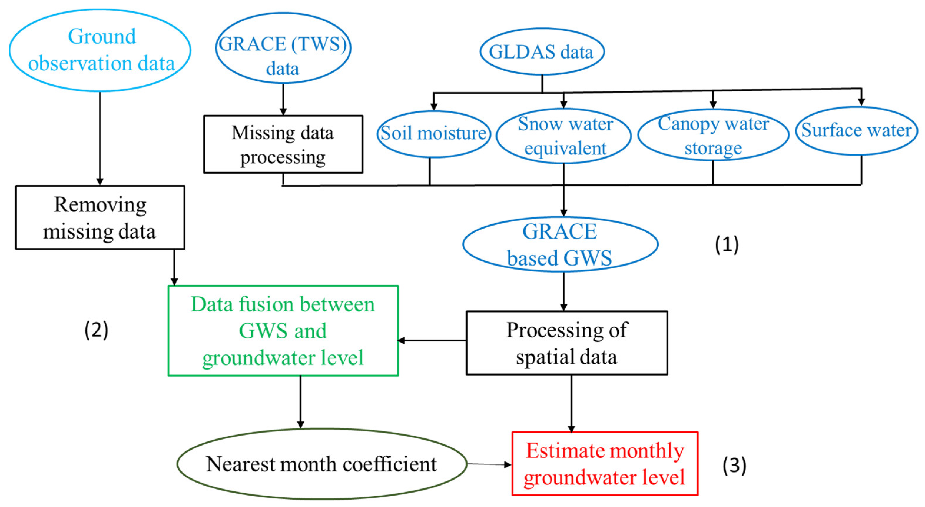
The Central Ground Water Board (CGWB) freely provides the seasonal data from groundwater monitoring wells, e.g., the depth to groundwater level. The groundwater level data were monitored in January (late post-monsoon), May (pre-monsoon), August (monsoon), and November (early post-monsoon) every year. Based on the data, the seasonal analysis has been performed for groundwater level change.
In the study area, more than 6300 well data are checked for consistency and missing values. Many wells with missing values or incomplete data occur in the study period in India. Eventually, 1430 well observations are used after data cleaning. For the modelling, the training and further testing data are prepared independently for data fusion (70% and 30% data for training and testing).

2.3. Methods

The data fusion flowchart is shown in Figure 2. For data preprocessing, the one-month-missing TWS data were linearly interpolated. The in situ observations with missing data on one or more seasons were excluded from the analysis. The methodology contains three sections. First, the monthly GWS changes are identified using the GRACE TWS and GLDAS datasets. For the second section, the spatial regression models between the GWS changes and groundwater levels are generated at four observed months. Eventually, for the estimation, the monthly groundwater levels are estimated based on the GWS data.

2.3.1. Monthly Groundwater Storage Change (ΔGWS)

The variation in TWS anomalies can be explained by water storage parameter changes. The expected changes to the TWS represent the mass variability in a key portion of hydrological components. The GLDAS data can help us to separate those hydrological components from the total TWS and understand the spatial and temporal variability of the groundwater storage [9,13,29]. The GLDAS input parameters (SM, SWE, SW, and CWS) are converted to an equivalent water height anomaly by removing the value of every individual parameter with temporal means between 2004–2009. Here, Equation (1) shows the total sum of all the storage changes in comparison to TWS changes.
ΔTWS = ΔSM + ΔSWE + ΔSW + ΔCWS + ΔGWS
where ΔSM is soil moisture change, ΔSWE is snow water equivalent change, ΔSW is surface water change, ΔCWS is canopy water storage change, and ΔGWS is groundwater storage change. The GWS change from TWS-based GRACE signals can be identified using Equation (2).
ΔGWS = ΔTWS − (ΔSM + ΔSWE + ΔSW + ΔCWS)
ΔGWS can be determined using GRACE-based TWS minus the GLDAS parameters, i.e., ΔSM, ΔSWE, ΔSW, and ΔCWS [14,18,29,30]. Eventually, the GRACE-based ΔGWS is generated with a spatial resolution of 0.5 × 0.5 degrees. The GLDAS considers different hydrological components of LSMs. Various LSMs have been used by different researchers, but the Noah model from the GLDAS-based data is highly preferred by researchers [28]; therefore, the Noah model-based input parameters are used for GWS extraction in this study. The GLDAS input parameters units are converted from kg/m2 to centimeters to make them consistent with the GRACE-based TWS data. For conversion to cm, the original GLDAS layers are multiplied by 0.1 to obtain the output product of every layer.

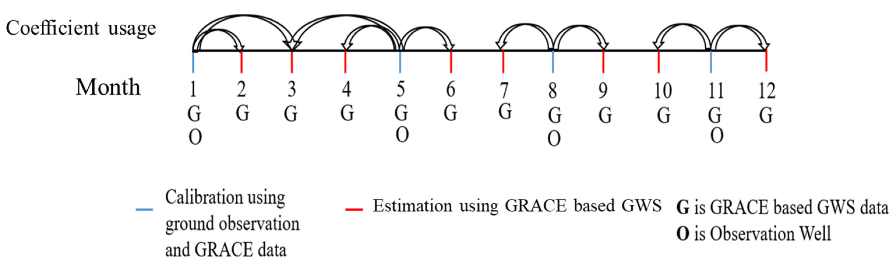
2.3.2. Data Fusion Using Time-Varying Spatial Regression

For estimation of the groundwater level from GRACE-based GWS, spatial regression has been used for data fusion. The time-varying spatial relation between GWS change and groundwater level at time t is shown in Equation (3).
h i , t = β 0 , t ( u i ,   v i ) + β 1 , t   ( u i ,   v i ) Δ GWS i , t + ε i , t ,
Here, h i , t is the estimation of the depth to groundwater level based on the groundwater storage change at location i at time t, Δ GWS i , t . β 0 , t ( u i   ,   v i ) is the intercept at every well location with latitude and longitude (ui, vi) [unit: m], β 1 , t ( u i   ,   v i ) is the slope coefficient at well location i at time t for Δ GWS [unit: m/cm], and ε i , t  is a residual error in the model [31,32]. In parameter estimation, the Δ GWS values at well locations are extracted using GIS. The spatial regression is applied to develop a monthly based groundwater level map determining the spatial pattern and its temporal variations in groundwater level based on GRACE-based monthly GWS changes. Spatial regression is the modified form of linear regression which considers the spatial weighted parameters.
The estimated parameter matrix β ^ k , t ( u i , v i ) = ( β 0 , t ( u i , v i ) , β 1 , t ( u i , v i ) ) T at time t for variable k is further determined using weighted least squares:
β ^ k , t ( u i , v i ) = [ X t T W ( u i , v i ) X t ] 1 X t T W ( u i , v i ) H t ,
X t = [ 1 Δ GWS 1 , t 1 Δ GWS n , t ] ,   H t = [ h 1 , t h n , t ] ,
W ( u i , v i ) is a spatially varying weight matrix developed from the Gaussian weighting function. The Gaussian weighting function is defined by well-known mathematical expression e ( D i j / b ) 2 , where b is the bandwidth, which is a non-negative parameter, and D i j is the distance between two observations of target i and its neighbor j. n is the observation number. Bandwidth is the key parameter of the Gaussian weighting function. The optimal bandwidth was estimated based on cross-validation in which the minimized errors between the observed and estimated values are determined to be as much as possible. In this study, the optimal bandwidth b is about 0.4. The regional monthly groundwater level can be estimated using GRACE-based GWS from Equation (3), after beta parameters are determined using Equations (4) and (5). Moreover, the beta parameter values of the GRACE-based GWS grids are interpolated for spatial groundwater level estimation.

2.3.3. Estimation of Monthly Groundwater Level

Groundwater monitoring is available for January, May, August, and November. The data fusion models are built using those four months. Then, the known spatial coefficients are used to estimate the spatial variation in groundwater level from the GWS. Based on the calibrated coefficients from Equations (4) and (5) during the observed months, spatial maps of the groundwater level during unobserved months are estimated. Figure 3 shows how to estimate the groundwater level map based on the seasonal in situ observations and monthly GRACE-based GWS. Firstly, the regression coefficients of the four months can be calibrated and determined. These regression coefficients are the priori information for data fusion. The coefficients of the unobserved months were obtained from the nearest neighboring observed month or computed as the average values of the two observed neighboring months. For example, the average values of coefficients in January and May were used for the estimation of the groundwater level in March.

3. Results

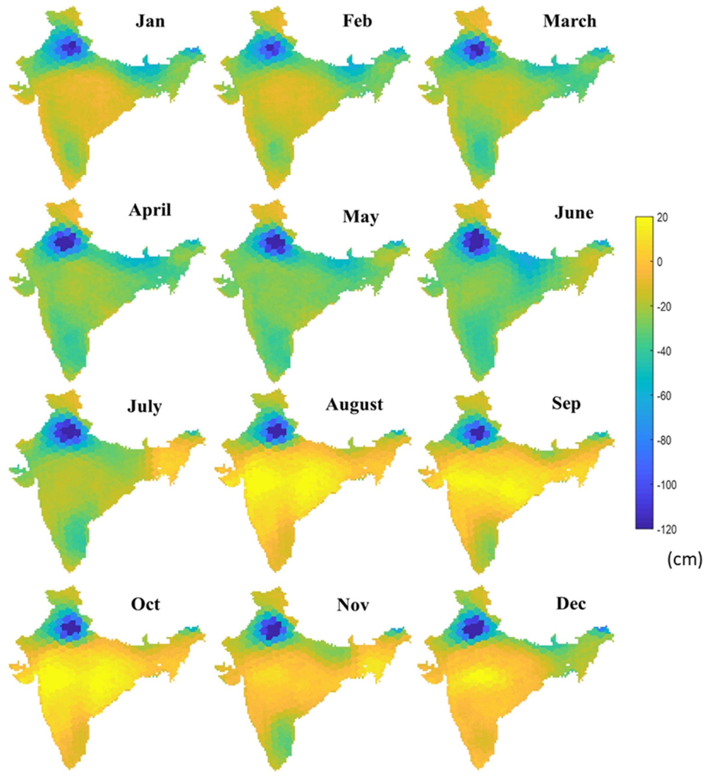
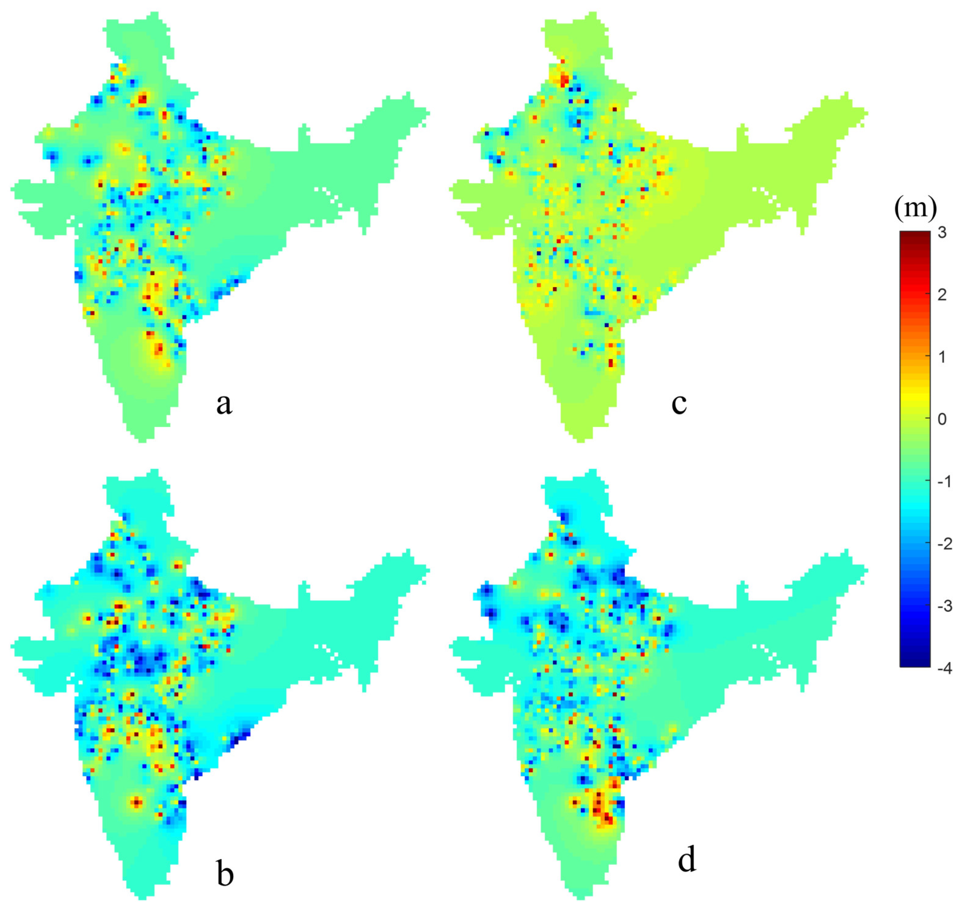
3.1. Spatio-Temporal Mapping of Monthly GWS Variation

Figure 4 shows the monthly based GWS spatial variations in 2019 relative to a 2004–2009 time–mean baseline for the study area of India and Bangladesh. The most severely affected area is the Northeast area. The groundwater depletion areas are mostly agricultural areas, where groundwater is used for irrigation so that groundwater storage decreases drastically [4,15]. As the hotspot area is mostly used for the agriculture of wheat and rice, most of the extraction of groundwater is used for irrigation purposes. Groundwater levels contain seasonal fluctuation. During the months from December to April, irrigation proposes that groundwater is the main source of water [33]. The heavy groundwater extraction period is in the first few months of the year. Panda and Wahr [19] conducted a study of annual groundwater depletion and found that the northern part of India, which was the largest storage area, has been the most continuously affected part for more than a decade. The monsoon season in the southern part of India is mostly between September and October and also extends to November in some years. Due to the high consumption of groundwater in pre-monsoon months, the lowest GWS values occur in this period, while the GWS values are at peak during and after the monsoon season [10]. The climatic variables, such as precipitation and evapotranspiration, cause seasonality effects on groundwater storage change [34]. Long-term variations in precipitation may affect groundwater storage in north India [35]. Guhathakurta and Rajeevan [36] found that the entirety of India receives >74% precipitation during the monsoon season (June to September). Groundwater storage variability in northwestern India can be explained predominantly by variability in groundwater extraction for irrigation, as well as also being influenced by changes in declining precipitation [35].

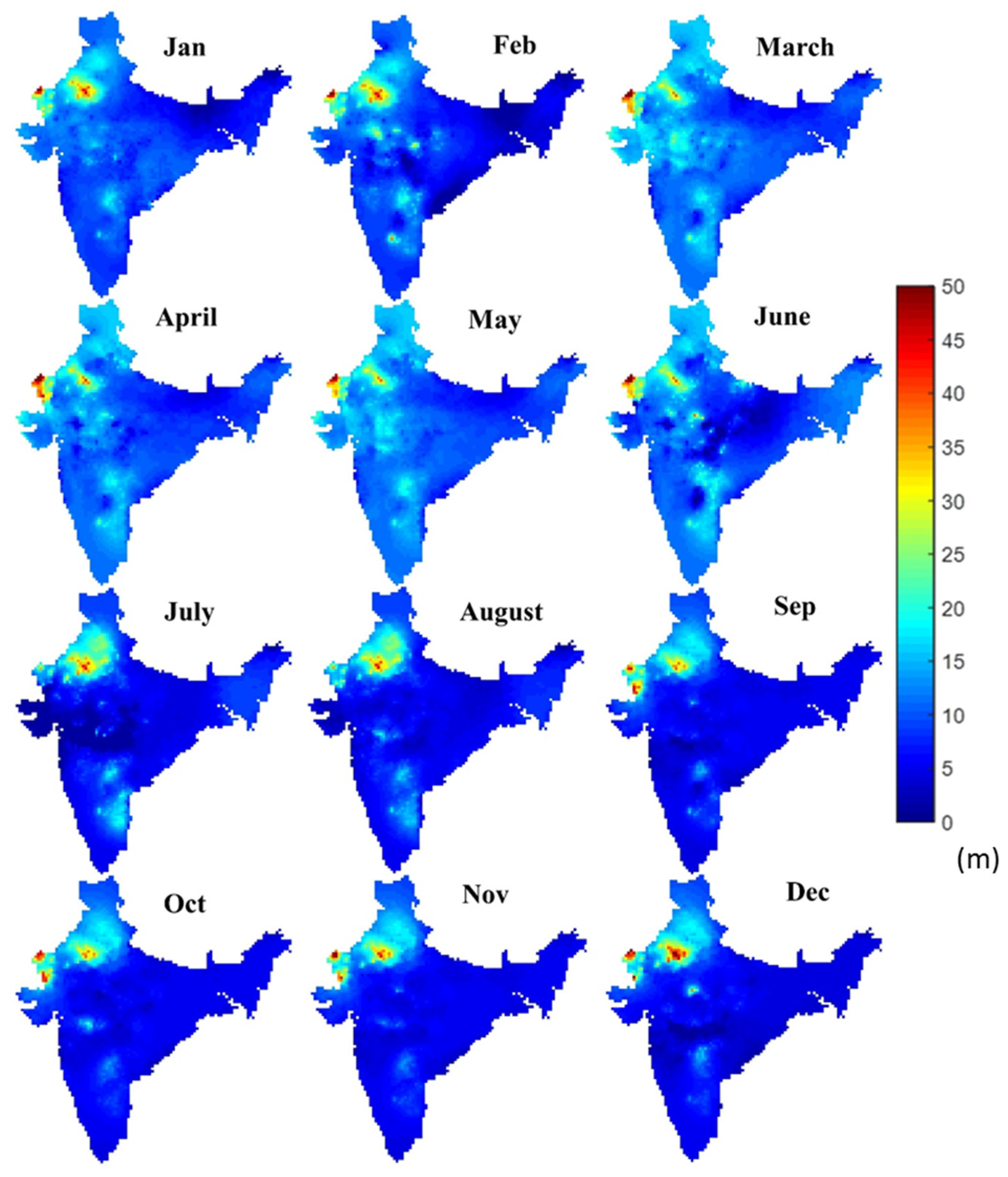
3.2. Monthly Spatial Groundwater Level Estimation

Figure 5 shows the monthly estimation maps of groundwater in 2019. The spatial and temporal variations in groundwater level can be identified using Equations (3)–(5). The results indicate that the northern area of India has a higher depth of groundwater level compared to the southern part. In the northern area, the depth of the groundwater level can reach from 50 to 55 m below the earth’s surface, while in the southern part, the level is only 15 to 20 m below the ground. Chen et al. [4] conducted a study on long-term groundwater variations in India and found that northwest India has a decreasing trend in groundwater storage, which further leads to groundwater level depletion in the area and also the surrounding areas of northern India. As the consumption of groundwater is high in the first months, the lowest groundwater level can be identified at around 55 m below the ground, and in the months of the monsoon season, the groundwater level starts to recover from September onwards. After the monsoon season, consumption of groundwater reduces. The depth of the groundwater level in the winter season rises, and the groundwater level extends to a range of between 40 to 45 m below the ground during the months of the winter season. The consumption of groundwater increases at the start of the year, and the groundwater level decreases due to high groundwater extraction. In Figure 5, results show that the groundwater level is very low in northern India, which further adds to depletion problems in terms of water resources. This approach not only shows the hotspots of the groundwater depletion, but also the spatio-temporal pattern variations in groundwater changes. The seasonal variations from climate and groundwater exploitation affect groundwater changes.
For the validation of groundwater level estimation, the RMSE (root mean square error) was calculated from the field observation and the estimation of the model in Table 1. The estimated values were extracted by the locations of observation wells in January, May, August, and November, during 2019. The average RMSE for groundwater level is 2.37 m. Figure 6 shows the groundwater level residual maps in (a) January, (b) May, (c) August, and (d) November, during 2019. Spatial residuals are randomly distributed. This represents the good performance of the estimation, since spatial regression usually reduces the spatial autocorrelation of model residuals. Furthermore, our future work will consider machine learning or deep learning approaches as data fusion models to reduce overall model residuals.

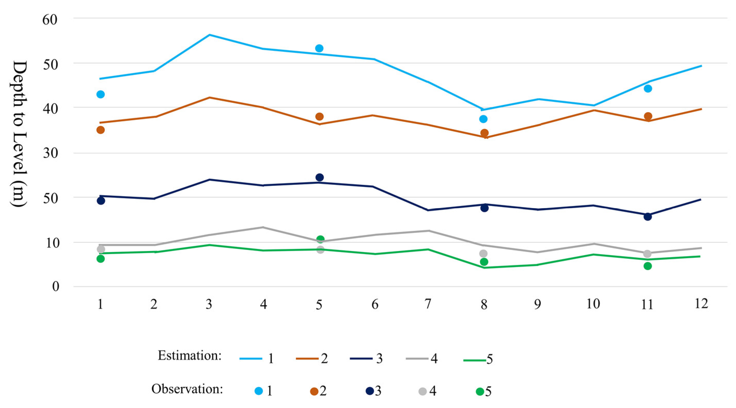
3.3. Time Series Plots for Validation

Figure 7 shows the multiple time series of groundwater levels below the earth surface in the checkpoints (red points in Figure 1). Results show the monthly estimated and seasonal observed groundwater levels when combining the GWS information. The groundwater level varies moderately in locations 3 and 5 (South India) when compared with location 1 and 2 (Northwest India). The groundwater levels vary seasonally, especially in Northwest India. The low peak of the groundwater level took place in March or April, but the high peak happened in August. This is highly related to agricultural activity. Northwest India is a hotspot area for groundwater depletion. The groundwater depletion in Northwest India is reported to be related to irrigation water withdrawals. Here, wheat and rice are planted and irrigated using groundwater extracted in the cropping seasons. The crops are sown in winter from October to December and harvested in summer from April to June. In addition, groundwater is the major source of water for irrigating crops here from December to April [33].
Considering these groundwater level estimations, groundwater management should be given attention in March because that is the month with the lowest groundwater level in the hotspot area. The volume of exploited groundwater increases between March and May because farmers start irrigating for cultivation. The groundwater level continues to increase to the highest level in August due to the monsoon. From October to January in the following year, the groundwater level becomes lower because groundwater exploitation remains at a high level. Application of the GRACE-derived GWS anomalies to estimate monthly groundwater level changes in India is validated based on the observation data. The robust spatial regression method used in this study provides the transformation from GWS to groundwater level. In addition, the lack of field measurements of aquifer storage properties causes extra uncertainties in the prediction of groundwater changes [37]. Currently, the estimation is determined from the coefficient of the neighboring month, but it could be used from the ones with the highest correlation in the future.

4. Discussion

4.1. Fusion of GRACE and Groundwater Level Data

The lack of integrity and continuity in groundwater level changes occurs only when using seasonal observations. Data scientists can use interpolation methods to develop reasonable guesses for groundwater variations. However, transferring from seasonal data to monthly data is still challenging. The monthly GRACE-based GWS changes provide sufficient information on the temporal groundwater variations in the study area. Generally, the transformation from GWS change to groundwater level is a spatial function [24]. Groundwater level maps can be obtained from spatial regression-based data fusion. The data fusion model is performed to discover the spatial pattern of groundwater changes. Essentially, the data fusion model is built to estimate the regional groundwater level using the GRACE data. We aim to increase the temporal resolution of groundwater level by using a data fusion approach while considering spatial relations between groundwater level and storage changes. This data fusion approach proposed here provides a reliable spatiotemporal representation, e.g., the temporal pattern and spatial heterogeneity of the groundwater changes.
Furthermore, data fusion for downscaling refers to a spatial resolution or temporal resolution increase within the datasets. Statistical models account for the downscaling processes within or across scales. Most GRACE downscaling studies were conducted by considering the auxiliary variables that were highly correlated with precipitation. GRACE-derived GWS was also used as the auxiliary variables and initial conditions, and the downscaling could be implemented. A statistic or dynamic downscaling algorithm produced high spatial resolution GWS changes from the GRACE data [38,39]. A high spatial resolution GWS or a groundwater level map was produced by utilizing the relationship between TWS and hydro-climatic variables using machine learning, e.g., a regression tree [17,33]. To increase the model performance, we will consider machine learning or deep learning approaches as data fusion models in the future.

4.2. Seasonality and Depletion Trend of Groundwater

GRACE provides large-scale spatio-temporal variations in GWS changes at the precision of tens of mm in equivalent water height. The GRACE-based GWS changes are consistent with the variations in groundwater levels [39]. The GRACE-based GWS shows the area-averaged signature of groundwater changes within the area. The result matches the finding from the GRACE-based model by [10]. In India, groundwater is the major source of water for irrigating crops [40]. The seasonality and depletion trend of GWS changes are due to the usage of groundwater for irrigation. Groundwater extraction has increased from 231 billion m3 in 2004 to 249 billion m3 in 2017. However, the usage for irrigation in a percentage for whole extraction has reduced from 92% to 89% during these years [41]. In addition, climate change directly influences precipitation variations and then seriously affects surface water and groundwater, especially during periods of drought. Heavy groundwater pumping for irrigation caused rapid groundwater depletion in India during persistent droughts. Precipitation variation is associated with the trends and patterns of GWS changes [42]. The irrigation from groundwater helps meet the rising food demands under climate changes but results in severe groundwater depletion in India.
The fusion model may obtain the global trend, but it loses the local variation in groundwater level. The uncertainty of groundwater estimation is large due to the fusion data resolution inconsistence, i.e., the coarse resolution of the original GRACE data. In addition, the changes in regional hydrology due to glacier mass balances are not simulated by using the GLDAS model. This glacier mass loss may have an effect on the GWS estimates, especially on the northern side of the area [37,38,39]. In the future, multiple global models and GRACE mascon products will be applied for comparison and validation.

5. Conclusions

The focus of this study is to develop a spatial regression-based data fusion model for estimating monthly groundwater levels. When field observations from groundwater monitoring wells are available only at a seasonal scale, the monthly variations in GRACE-based groundwater storage (GWS) are further used to estimate the spatial maps of monthly groundwater levels. The spatial estimated coefficients are used for the spatial estimations at the months without groundwater observations.
The estimated groundwater level is further validated in the groundwater monitoring wells data, showing an average RMSE of 2.37 m. Using this approach in groundwater monitoring, patterns of regional groundwater levels are reliable to understand groundwater spatio-temporal variability. Result shows that the groundwater level is 50 to 55 m below the ground in northern India. The groundwater level rises to 40 to 45 m below the ground in the northern part during the monsoon season. Groundwater level monitoring and control is critical in northern India, where groundwater extraction is important for sustaining agricultural activities. Moreover, these results will be further used for the mitigation of groundwater depletion. Groundwater managers and government authorities can apply the model to identify the groundwater level distribution for groundwater control. The effective monitoring wells will be selected for validation. In the future, we will check the uncertainty of the currently employed nearest-month coefficient approach and compare this approach with a linear interpolator to estimate the time-dependent coefficients from the GRACE data for groundwater mapping. In addition, machine learning or deep learning approaches as data fusion models will be considered.

Author Contributions

Conceptualization, H.-J.C.; methodology, H.-J.C. and M.Z.A.; validation, M.Z.A.; formal analysis, M.Z.A. and T.; writing—original draft preparation, M.Z.A.; writing—review and editing, H.-J.C.; visualization, M.Z.A.; supervision, H.-J.C. All authors have read and agreed to the published version of the manuscript.

Funding

The funding that support the findings of this study are partly available from SATU Joint Research Scheme, and Ministry of Science and Technology (MOST), Taiwan.

Institutional Review Board Statement

Not applicable.

Informed Consent Statement

Not applicable.

Data Availability Statement

The data that support the findings of this study are available from Center for Space Research (CSR) at University of Texas at Austin, from NASA in Land Surface Models, and from India Water Resources Information System, Department of Water Resources, India.

Acknowledgments

The authors would like to thank GeoSmart Lab members and coworkers: Kurmar, Aman, Mita and Sumriti, and C-W Hwang for providing suggestions for paper improvement.

Conflicts of Interest

The authors declare that they have no known competing financial interests or personal relationships that could have appeared to influence the work reported in this paper.

Appendix A

Table A1. Locations of checkpoints in this study.
Well ID in Figure 1Latitude (Degree)Longitude (Degree)
127.62274.367
227.23870.444
314.87077.566
424.42478.078
517.89873.855

References

  1. Gleeson, T.; VanderSteen, J.; Sophocleous, M.A.; Taniguchi, M.; Alley, W.M.; Allen, D.M.; Zhou, Y. Groundwater sustainability strategies. Nat. Geosci. 2010, 3, 378–379. [Google Scholar] [CrossRef]
  2. Scanlon, B.R.; Longuevergne, L.; Long, D. Ground referencing GRACE satellite estimates of groundwater storage changes in the California Central Valley, USA. Water Resour. Res. 2012, 48, 1–9. [Google Scholar] [CrossRef]
  3. Wang, Y.; Chen, Z.-Y. Responses of groundwater system to water development in northern China. J. Groundw. Sci. Eng. 2016, 4, 69–80. [Google Scholar]
  4. Chen, J.; Li, J.; Zhang, Z.; Ni, S. Long-term groundwater variations in Northwest India from satellite gravity measurements. Glob. Planet. Chang. 2014, 116, 130–138. [Google Scholar] [CrossRef]
  5. Galloway, D.L.; Hudnut, K.W.; Ingebritsen, S.E.; Phillips, S.P.; Peltzer, G.; Rogez, F.; Rosen, P.A. Detection of aquifer system compaction and land subsidence using interferometric synthetic aperture radar, Antelope Valley, Mojave Desert, California. Water Resour. Res. 1998, 34, 2573–2585. [Google Scholar] [CrossRef]
  6. Phien-Wej, N.; Giao, P.; Nutalaya, P. Land subsidence in Bangkok, Thailand. Eng. Geol. 2006, 82, 187–201. [Google Scholar] [CrossRef]
  7. Abidin, H.Z.; Andreas, H.; Djaja, R.; Darmawan, D.; Gamal, M. Land subsidence characteristics of Jakarta between 1997 and 2005, as estimated using GPS surveys. GPS Solut. 2008, 12, 23–32. [Google Scholar] [CrossRef]
  8. Tapley, B.D.; Bettadpur, S.; Ries, J.C.; Thompson, P.F.; Watkins, M.M. GRACE Measurements of Mass Variability in the Earth System. Science 2004, 305, 503–505. [Google Scholar] [CrossRef]
  9. Famiglietti, J.S.; Rodell, M. Water in the balance. Science 2013, 340, 1300–1301. [Google Scholar] [CrossRef]
  10. Bhanja, S.N.; Mukherjee, A.; Saha, D.; Velicogna, I.; Famiglietti, J.S. Validation of GRACE based groundwater storage anomaly using in-situ groundwater level measurements in India. J. Hydrol. 2016, 543, 729–738. [Google Scholar] [CrossRef]
  11. Rodell, M.; Houser, P.R.; Jambor, U.; Gottschalck, J.; Mitchell, K.; Meng, C.-J.; Arsenault, K.; Cosgrove, B.; Radakovich, J.; Bosilovich, M.; et al. The Global Land Data Assimilation System. Bull. Am. Meteorol. Soc. 2004, 85, 381–394. [Google Scholar] [CrossRef]
  12. Tiwari, V.M.; Wahr, J.; Swenson, S. Dwindling groundwater resources in northern India, from satellite gravity observations. Geophys. Res. Lett. 2009, 36, 1–5. [Google Scholar] [CrossRef]
  13. Voss, K.A.; Famiglietti, J.S.; Lo, M.-H.; De Linage, C.; Rodell, M.; Swenson, S.C. Groundwater depletion in the Middle East from GRACE with implications for transboundary water management in the Tigris-Euphrates-Western Iran region. Water Resour. Res. 2013, 49, 904–914. [Google Scholar] [CrossRef]
  14. Richey, A.S.; Thomas, B.F.; Lo, M.-H.; Reager, J.T.; Famiglietti, J.S.; Voss, K.; Swenson, S.; Rodell, M. Quantifying renewable groundwater stress with GRACE. Water Resour. Res. 2015, 51, 5217–5238. [Google Scholar] [CrossRef]
  15. Hora, T.; Srinivasan, V.; Basu, N.B. The Groundwater Recovery Paradox in South India. Geophys. Res. Lett. 2019, 46, 9602–9611. [Google Scholar] [CrossRef]
  16. Döll, P.; Hoffmann-Dobrev, H.; Portmann, F.; Siebert, S.; Eicker, A.; Rodell, M.; Strassberg, G.; Scanlon, B. Impact of water withdrawals from groundwater and surface water on continental water storage variations. J. Geodyn. 2012, 59–60, 143–156. [Google Scholar] [CrossRef]
  17. Xiong, J.; Abhishek; Guo, S.; Kinouchi, T. Leveraging machine learning methods to quantify 50 years of dwindling groundwater in India. Sci. Total. Environ. 2022, 835, 155474. [Google Scholar] [CrossRef]
  18. Famiglietti, J.S.; Lo, M.; Ho, S.L.; Bethune, J.; Anderson, K.J.; Syed, T.H.; Swenson, S.C.; de Linage, C.R.; Rodell, M. Satellites Measure Recent Rates of Groundwater Depletion in California’s Central Valley. Geophys. Res. Lett. 2011, 38, L03403. [Google Scholar] [CrossRef]
  19. Panda, D.K.; Wahr, J. Spatiotemporal evolution of water storage changes in I ndia from the updated GRACE -derived gravity records. Water Resour. Res. 2016, 52, 135–149. [Google Scholar] [CrossRef]
  20. Mohamed, A.; Abdelrady, A.; Alarifi, S.S.; Othman, A. Geophysical and Remote Sensing Assessment of Chad’s Groundwater Resources. Remote. Sens. 2023, 15, 560. [Google Scholar] [CrossRef]
  21. Alshehri, F.; Mohamed, A. Analysis of Groundwater Storage Fluctuations Using GRACE and Remote Sensing Data in Wadi As-Sirhan, Northern Saudi Arabia. Water 2023, 15, 282. [Google Scholar] [CrossRef]
  22. Mohamed, A.; Othman, A.; Galal, W.F.; Abdelrady, A. Integrated Geophysical Approach of Groundwater Potential in Wadi Ranyah, Saudi Arabia, Using Gravity, Electrical Resistivity, and Remote-Sensing Techniques. Remote. Sens. 2023, 15, 1808. [Google Scholar] [CrossRef]
  23. Scanlon, B.R.; Zhang, Z.; Save, H.; Sun, A.Y.; Schmied, H.M.; van Beek, L.P.H.; Wiese, D.N.; Wada, Y.; Long, D.; Reedy, R.C.; et al. Global models underestimate large decadal declining and rising water storage trends relative to GRACE satellite data. Proc. Natl. Acad. Sci. USA 2018, 115, E1080–E1089. [Google Scholar] [CrossRef] [PubMed]
  24. Chu, H.-J.; Wijayanti, R.F.; Jaelani, L.M.; Tsai, H.-P. Time Varying Spatial Downscaling of Satellite-Based Drought Index. Remote. Sens. 2021, 13, 3693. [Google Scholar] [CrossRef]
  25. Gupta, S.D.; Mukherjee, A.; Bhattacharya, J. Groundwater of South Asia; Springer Hydrogeol: Berlin/Heidelberg, Germany, 2018; pp. 247–255. [Google Scholar]
  26. Margat, J.; van der Gun, J. Groundwater around the World: A Geographic Synopsis; CRC Press: Boca Raton, FL, USA, 2013. [Google Scholar]
  27. Central Water Commission (CWC); National Remote Sensing Centre (NRSC). Watershed Atlas of India; 2014. Available online: https://www.researchgate.net/publication/316663108_WATERSHED_ATLAS_OF_INDIA?channel=doi&linkId=590ab9380f7e9b1d0823ec7a&showFulltext=true (accessed on 5 April 2023).
  28. Hussain, D.; Kao, H.-C.; Khan, A.A.; Lan, W.-H.; Imani, M.; Lee, C.-M.; Kuo, C.-Y. Spatial and Temporal Variations of Terrestrial Water Storage in Upper Indus Basin Using GRACE and Altimetry Data. IEEE Access 2020, 8, 65327–65339. [Google Scholar] [CrossRef]
  29. Purdy, A.J.; David, C.H.; Sikder, S.; Reager, J.T.; Chandanpurkar, H.A.; Jones, N.L.; Matin, M.A. An Open-Source Tool to Facilitate the Processing of GRACE Observations and GLDAS Outputs: An Evaluation in Bangladesh. Front. Environ. Sci. 2019, 7, 155. [Google Scholar] [CrossRef]
  30. Han, J.; Tangdamrongsub, N.; Hwang, C.; Abidin, H.Z. Intensified water storage loss by biomass burning in Kalimantan: Detection by GRACE. J. Geophys. Res. Solid Earth 2017, 122, 2409–2430. [Google Scholar] [CrossRef]
  31. Fotheringham, A.S.; Brunsdon, C.; Charlton, M. Geographically weighted regression: The analysis of spatially varying relationships. Educ. Psychol. Meas. 2002, 31, 1029. [Google Scholar] [CrossRef]
  32. Ali, M.Z.; Chu, H.-J.; Burbey, T.J. Mapping and predicting subsidence from spatio-temporal regression models of groundwater-drawdown and subsidence observations. Hydrogeol. J. 2020, 28, 2865–2876. [Google Scholar] [CrossRef]
  33. Watkins, M.M.; Wiese, D.N.; Yuan, D.-N.; Boening, C.; Landerer, F.W. Improved methods for observing Earth’s time variable mass distribution with GRACE using spherical cap mascons. AGU J. Geophys. Res. Solid Earth 2015, 120, 2648–2671. [Google Scholar] [CrossRef]
  34. Eltahir, E.A.B.; Yeh, P.J.-F. On the asymmetric response of aquifer water level to floods and droughts in Illinois. Polygr. Int. 1999, 35, 1199–1217. [Google Scholar] [CrossRef]
  35. Asoka, A.; Gleeson, T.; Wada, Y.; Mishra, V. Relative contribution of monsoon precipitation and pumping to changes in groundwater storage in India. Nat. Geosci. 2017, 10, 109–117. [Google Scholar] [CrossRef]
  36. Guhathakurta, P.; Rajeevan, M. Trends in the rainfall pattern over India. Int. J. Climatol. 2008, 28, 1453–1469. [Google Scholar] [CrossRef]
  37. Neves, M.C.; Nunes, L.M.; Monteiro, J.P. Evaluation of GRACE data for water resource management in Iberia: A case study of groundwater storage monitoring in the Algarve region. J. Hydrol. Reg. Stud. 2020, 32, 100734. [Google Scholar] [CrossRef]
  38. Seyoum, W.M.; Kwon, D.; Milewski, A.M. Downscaling GRACE TWSA Data into High-Resolution Groundwater Level Anomaly Using Machine Learning-Based Models in a Glacial Aquifer System. Remote. Sens. 2019, 11, 824. [Google Scholar] [CrossRef]
  39. Sun, J.; Hu, L.; Liu, X.; Sun, K. Enhanced Understanding of Groundwater Storage Changes under the Influence of River Basin Governance Using GRACE Data and Downscaling Model. Remote Sens. 2022, 14, 4719. [Google Scholar] [CrossRef]
  40. Dangar, S.; Asoka, A.; Mishra, V. Causes and implications of groundwater depletion in India: A review. J. Hydrol. 2021, 596, 126103. [Google Scholar] [CrossRef]
  41. Saha, D.; Marwaha, S.; Dwivedi, S. Role of Measuring the Aquifers for Sustainably Managing Groundwater Resource in India. In Global Groundwater; Elsevier: Amsterdam, The Netherlands, 2020; pp. 477–486. [Google Scholar] [CrossRef]
  42. Swain, S.; Taloor, A.K.; Dhal, L.; Sahoo, S.; Al-Ansari, N. Impact of climate change on groundwater hydrology: A comprehensive review and current status of the Indian hydrogeology. Appl. Water Sci. 2022, 12, 120. [Google Scholar] [CrossRef]
Figure 1. Study area; locations of training and testing samples, and time series checkpoints for groundwater level mapping.
Sustainability 15 08295 g001
Figure 2. Methodological workflow for a research study. (1) monthly GWS changes are identified using GRACE and GLDAS datasets; (2) spatial regression models between the monthly GWS changes and groundwater levels are generated; (3) monthly groundwater levels are estimated based on GRACE data from nearest-month coefficients.
Sustainability 15 08295 g002
Figure 3. Monthly estimation of groundwater level using GRACE-based GWS and calibrated coefficients from neighboring observed months.
Sustainability 15 08295 g003
Figure 4. Monthly spatial distribution of groundwater storage anomalies for a 1-year cycle from GRACE CSR data in 2019 relative to a 2004–2009 time–mean baseline.
Sustainability 15 08295 g004
Figure 5. Monthly spatial estimation maps of groundwater level depth in 2019 from GRACE-based GWS.
Sustainability 15 08295 g005
Figure 6. Model residual interpolated maps in (a) January, (b) May, (c) August, and (d) November, during 2019.
Sustainability 15 08295 g006
Figure 7. Monthly estimated and seasonal observed groundwater level depth in 2019 at five stations (red points in Figure 1, longitude and latitude are shown in Appendix A).
Sustainability 15 08295 g007
Table 1. RMSE of estimated groundwater depth for validation.
MonthRMSE (m)
January2.24
May2.80
August1.94
November2.49
Average2.37
Disclaimer/Publisher’s Note: The statements, opinions and data contained in all publications are solely those of the individual author(s) and contributor(s) and not of MDPI and/or the editor(s). MDPI and/or the editor(s) disclaim responsibility for any injury to people or property resulting from any ideas, methods, instructions or products referred to in the content.

