Energy Performance Analysis of Photovoltaic Integrated with Microgrid Data Analysis Using Deep Learning Feature Selection and Classification Techniques

Abstract

Microgrids are an essential element of smart grids, which contain distributed renewable energy sources (RESs), energy storage devices, and load control strategies. Models built based on machine learning (ML) and deep learning (DL) offer hope for anticipating consumer demands and energy production from RESs. This study suggests an innovative approach for energy analysis based on the feature extraction and classification of microgrid photovoltaic cell data using deep learning algorithms. The energy optimization of a microgrid was carried out using a photovoltaic energy system with distributed power generation. The data analysis has been carried out for feature analysis and classification using a Gaussian radial Boltzmann with Markov encoder model. Based on microgrid energy optimization and data analysis, an experimental analysis of power analysis, energy efficiency, quality of service (QoS), accuracy, precision, and recall has been conducted. The proposed technique attained power analysis of 88%, energy efficiency of 95%, QoS of 77%, accuracy of 93%, precision of 85%, and recall of 77%.

1. Introduction

Current demand for energy consumption is predicated on burning fossil fuels to provide dependable and resilient energy networks. Unquestionably, one of the most significant issues for scientists and engineers is the requirement for energy. Energy production techniques from the preceding century are now acknowledged as being inappropriate because of rising atmospheric carbon dioxide (CO₂) emissions [1]. The significant contribution of non-renewable energy sources raises environmental issues since they release greenhouse gases into the atmosphere, which have detrimental effects on human health and the ecosystem. As they are generally accessible, clean, and free of pollution, renewable energy sources (RESs) have gained popularity and attention across the globe. By 2030, it is anticipated that RESs like wind, solar, hydro, geothermal, and biomass would dominate world’s electricity production and surpass all other energy sources [2]. Among the renewables, photovoltaics have experienced the fastest increase over the past few decades. Currently, wind energy production exceeds that of photovoltaic (PV), although PV is more widely accessible and wind turbines require extremely specialized site conditions. As an alternative, photovoltaics have become a viable option in the fight against climate change. The process of turning light into electricity using semiconducting materials that display the photovoltaic effect is known as photovoltaic (PV). The three main PV cell technologies—monocrystalline silicon, polycrystalline silicon, and thin film—control the global market. Among these, thin film solar cells offer several advantages over traditional silicon-based PV cells. They can be manufactured using low-cost techniques, such as roll-to-roll deposition or printing methods, which can potentially reduce production costs and enable large-scale manufacturing. Thin film solar cells are also lightweight and flexible, making them suitable for various applications, including building-integrated photovoltaics, portable electronics, and off-grid installations. However, the efficiency of thin film solar cells is generally lower than that of silicon-based cells [3].

The amazing rise in human living standards and the resulting rise in electricity demand have led to a number of super-large-scale power system flaws that are now more obvious than ever [4]. The traditional fossil fuel-based power plants are unable to provide enough energy to keep up with the rising demand for electricity. Early in the twenty-first century, the idea of a microgrid (MG) for integrating clean renewable energy sources (RESs) was put forth. A small-scale local power system called a microgrid is made up of electric loads, control systems, and distributed energy resources (DERs). Energy storage systems (ESSs) and RERs are both used in the microgrid’s power generation or DERs. A new sort of contemporary active power distribution system for the use and advancement of renewable energy is the microgrid [5]. However, microgrids make it more challenging to maintain a balance between energy production and consumption, and the incorporation of RESs complicates power grid operations.

PV plant power generation frequently experiences significant fluctuations, including voltage irregularities, reserve power flow issues, and power distribution problems. Additionally, energy users show unpredictable usage of power due to a variety of factors, including alterations in the environment and user activity. Therefore, it is important to analyze the performance of the system to provide better consumer services and to maintain a reliable and sustainable system.

Accurate forecasting of PV panels is a challenging task since it depends only on the weather conditions such as temperature, humidity, etc. [6]. Prediction can be carried out using many techniques such as physical mode, machine learning (ML), and deep learning (DL) [2]. Each prediction method has its own advantages and disadvantages. Physical methods, for instance, can anticipate the shifting patterns of the environment with high precision, but they need a lot of processing capacity since they require a massive amount of data. Physical techniques encounter unforeseen estimating errors and are inappropriate for short-term forecasting horizons, which raises further problems. Similar to this, the majority of the statistical models used to anticipate renewable energy are linear in design, which restricts their application to forecasting issues with wider time horizons. ML-based prediction provides findings that are more accurate than those produced by statistical and physical methods owing to its data mining and feature extraction capabilities. However, ML-based prediction models require shallow models as the foundation of their learning strategies. Trees, regressors, and neural networks with zero or one hidden layer are examples of common shallow patterns. Often, extensive knowledge and expertise are needed while training such shallow models. Therefore, it is frequently difficult to investigate shallow structures theoretically. Hence, shallow models have certain disadvantages in real-world applications. Lately, it has been determined that DL-based approaches to energy generation and power load forecasting performed better than ML-based approaches. Unlike ML, DL-based methods do not have problems with manually chosen feature selection, complex samples, or ineffective generalization competence [7]. Consequently, it is impossible to ignore the dynamics of renewable resource energy generation behavior. The limited use of MGs in literature work prevents real-world data from being taken into account while controlling energy distribution. For better energy management of real-world data, a complete framework is needed. Furthermore, power trading between different market players is completely ignored, and prior statistical information of uncertain renewable resource energy production was assumed to be perfectly understood. This is the driving force behind the suggested method, which combines deep learning approaches with distributed energy management to enhance the effectiveness and dependability of the proposed system.

Objectives of this work are as follows:

• To propose novel method for energy analysis based on a microgrid photovoltaic system by feature extraction and classification using deep learning techniques.
• The energy optimization of a microgrid using a photovoltaic energy system with distributed power generation.
• The data analysis for feature analysis and classification using a Gaussian radial Boltzmann with Markov encoder model.

2. Related Works

The following is a list of the most significant research topics on energy management that have been studied over the course of the last few years. The research conducted in [8] examined the most effective way to manage energy in renewable microgrids by taking into consideration batteries, solar panels, and wind turbines. The work in [9] analyzes the impact that wind and solar hybrid power generation technologies have on the performance of a sustainable microgrid. It is illustrated that a larger penetration of hybrid renewable energy sources might bring possible answers, provided they are controlled in the appropriate manner. The effects of uncertainty that are connected with RESs may be simulated by utilizing a stochastic technique that is based on Monte Carlo as described in [10]. The administration and maintenance of renewable microgrids is discussed in [11] from the perspective of a data-driven paradigm. When it comes to microgrids, ref. [12] makes use of the same research, but this time with a concentration on WSNs. It has been discovered that a microgrid that runs on renewable energy sources and fitted with a number of sensors is susceptible to being hacked. The creation of hydrogen by a renewable microgrid and the recovery of thermal energy by a fuel cell are the topics of discussion in [13]. By adopting multi-objective switching, the power losses and related costs with renewable sources may be minimized and optimized, as shown in [14]. Research of a similar kind is shown in [15] with regard to the influence that switching has on the most appropriate management strategy and course of action for microgrids. In [16], the authors conducted an analysis to see how the functioning of microgrids will be impacted by electric cars. According to [17], it is important to estimate charging needs for electric cars based on a detailed inspection and analysis of their erratic conduct in a complex environment. In order to do this, it is necessary to examine and analyze the erratic behavior of electric vehicles. Ref. [18] goes into more detail on the advantages and disadvantages of these kinds of systems, as well research that is relevant to both. In most cases, the energy management system (EMS) is not just concerned with preserving the energy balance inside the microgrid but it also has additional objectives in mind. The reduction of operating expenses, pollutants, and losses might be among these aims, in addition to a great number of other objectives, the attainment of which is contingent on the reason for the creation of such systems. A good number of these management systems additionally integrate various objectives in a manner that is multi-objective [19]. The probabilistic solar radiation forecasting that was produced in [20] made use of an analogue ensemble approach. In [21], it was recommended that ensemble forecasting based on empirical biasing be used to anticipate the geographical as well as temporal day ahead total daily radiation. This would be possible via the use of empirical biasing. In [22], Las-so was used to provide a radiation prediction for the next 5 min.

3. System Model

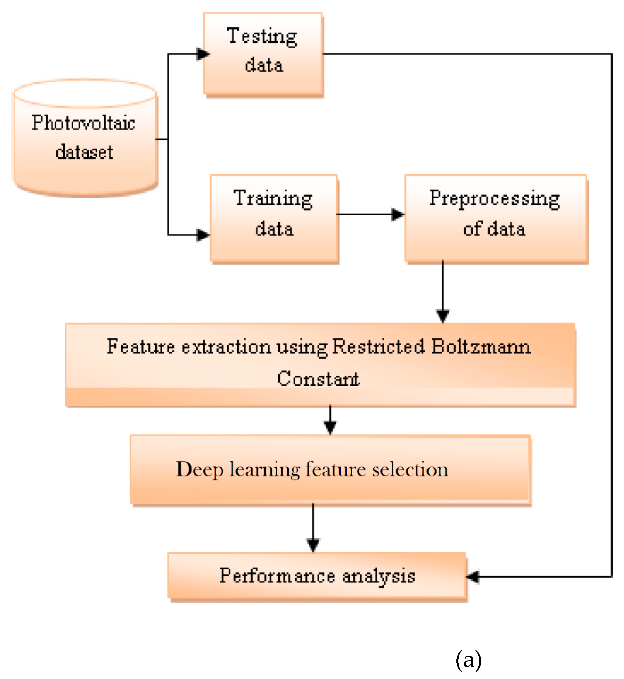
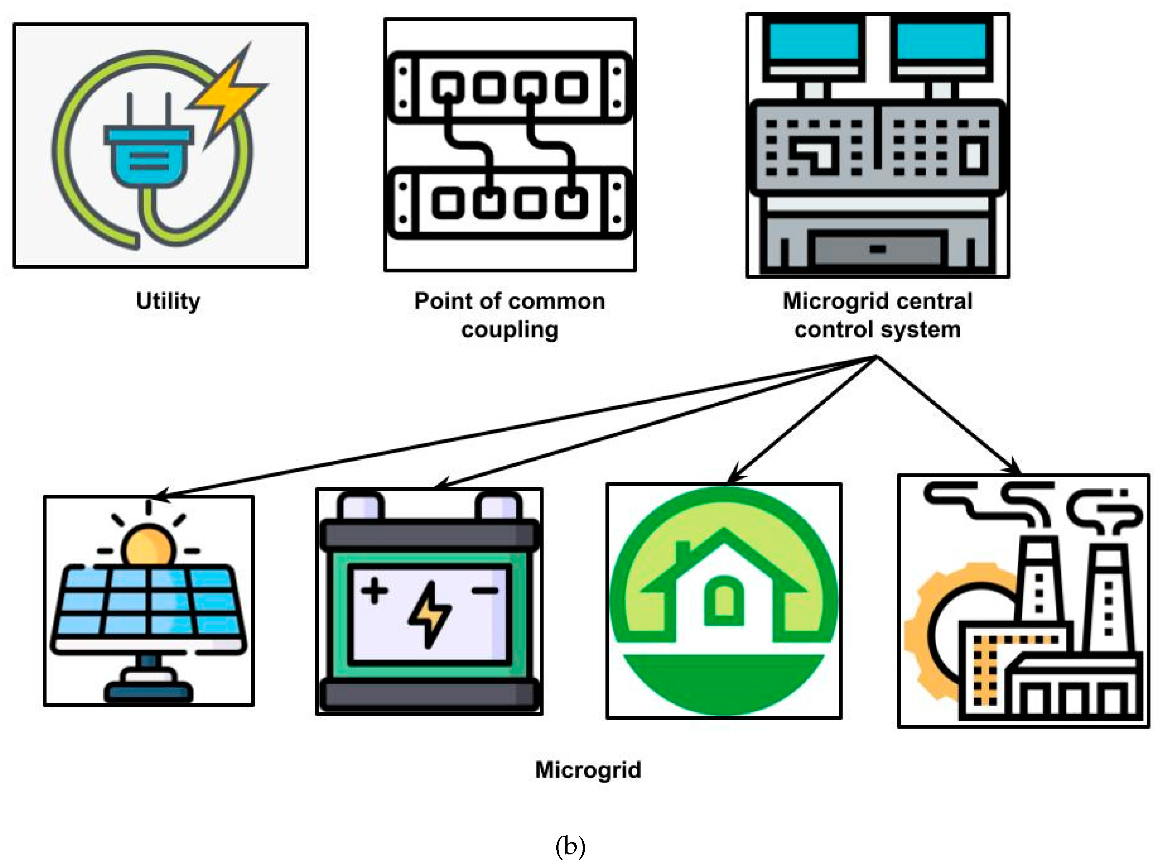
This section proposes a novel method in energy analysis based on microgrid photovoltaic cell data analysis by feature extraction and classification using deep learning techniques (Figure 1a). The energy optimization of the microgrid is carried out using a photovoltaic-based energy system with distributed power generation. The data analysis has been carried out for feature analysis and classification using a Gaussian radial Boltzmann with Markov encoder model. It is an algorithm for learning that assists individuals in finding intriguing characteristics hidden inside datasets that are made up of binary vectors. In networks with multiple layers of feature detectors, the learning process is often quite slow. However, the pace of the algorithm may be increased by adding a learning layer to the feature detectors in the network. The plug-and-play electric grid is one of the outstanding features of the microgrid since it can operate both independently and cooperatively with the power grids. The structural organization and linkages of the microgrid are shown in Figure 1b. With the capacity to choose the quantity and type of renewable energy sources that may be incorporated into the system, these tiny grids offer energy with improved stability, security, and resilience. It follows that microgrids have the capacity to effectively integrate a variety of diverse sources of distributed power generation, particularly renewable power sources. The microgrid is a small-scale local power system which integrates the clean renewable energy sources (RESs) made up of electric loads, control systems, and distributed energy resources (DERs). Energy storage systems (ESSs) and RERs are both used in a microgrid’s power generation or DERs. A new sort of contemporary active power distribution system for the use and advancement of renewable energy is the microgrid.

Photovoltaic-based energy system with distributed power generation:

The method is based on a series of newly developed 3D matrix-based equations that calculate the system’s overall load at the time of observation, the amount of power supplied to home DC, SLs from the utility’s main DC grid, and the efficiency of the entire system. Let “NT” be number of time samples within the observational period of time “T.” The following sets of indices, p q, and r, are provided in Equation (1) throughout the modeling.

$$\begin{gathered} \{\mathrm{superset} \mathrm{or} \mathrm{subset}\}= \\ \left\{\begin{array}{l}p\supseteq P_1=\{\mathrm{1,2},\dots ,x\}\mathrm{or}p\supset P_1^{\prime }=\{\mathrm{1,2},\dots ,x\}\\ q\supseteq Q=\{\mathrm{1,2},\dots ,y\}\mathrm{or}q\supset Q^{\prime }=\{\mathrm{1,2},\dots ,y\}\\ r\supseteq R=\{\mathrm{1,2},\dots ,n\}\mathrm{or}r\supset R^{\prime }=\{\mathrm{1,2},\dots ,n\}\end{array}\right\} \\ {L}_i={\sum }_{j=1}^N\left|V_i\right|\left|V_j\right|\mathrm{\angle }\left(G_{ij}\mathrm{c}\mathrm{o}\mathrm{s}\left({\phi }_i-{\phi }_j\right)+B_{ij}\mathrm{s}\mathrm{i}\mathrm{n}\left({\phi }_i-{\phi }_j\right)\right) \\ {M}_i={\sum }_{j=1}^N\left|V_i\right|\left|V_j\right|\mathrm{\angle }\left(G_{ij}\mathrm{s}\mathrm{i}\mathrm{n}\left({\phi }_i-{\phi }_j\right)-B_{ij}\mathrm{c}\mathrm{o}\mathrm{s}\left({\phi }_i-{\phi }_j\right)\right) \end{gathered}$$

(1)

where “x” is the largest number of possible loads in “y” and SL at the time “t_n” has maximum samples (“n”) in the system. The number “x” of DC loads that exist in the “y” MGs at time “t_n” is shown as (2). It is a huge 3D matrix of order [x, y] because each component of the matrix is a column matrix of NT of order 1.

$$\begin{gathered} {\mathrm{D}\mathrm{C}}_{\mathrm{L}\mathrm{y}\mathrm{M}\mathrm{G}\mathrm{s}}\left(t_n\right)={\left[{\left[p_{\mathrm{D}ij}\left(t_n\right)\right]}_{\mathrm{N}\mathrm{T}\times 1}\right]}_{x\times y} \\ \hspace{1em}\hspace{1em}\hspace{1em}\hspace{1em}\hspace{1em}\hspace{1em}\hspace{1em}\hspace{1em}\hspace{1em}\hspace{1em}\hspace{1em}\hspace{1em}\hspace{1em}\hspace{1em}=\left[\begin{array}{ccc}{\left[p_{\mathrm{D}11}\left(t_n\right)\right]}_{\mathrm{N}\mathrm{T}\times 1}& \cdots & {\left[p_{\mathrm{D}1y}\left(t_n\right)\right]}_{\mathrm{N}\mathrm{T}\times 1}\\ ⋮& \ddots & ⋮\\ {\left[p_{\mathrm{D}x1}\left(t_n\right)\right]}_{\mathrm{N}\mathrm{T}\times 1}& \cdots & {\left[p_{\mathrm{D}xy}\left(t_n\right)\right]}_{\mathrm{N}\mathrm{T}\times 1}\end{array}\right] \end{gathered}$$

(2)

This is [pD11 (t_n)]. The power of the first DC load present in the first MG at time “t_n” is represented by the column matrix NT × 1, which is further enlarged as Equation (3).

$$\begin{gathered} {\left[p_{\mathrm{D}ij}\left(t_n\right)\right]}_{\mathrm{N}\mathrm{T}\times 1}={\left[\begin{array}{c}{p}_{\mathrm{D}ij}\left(t_1\right)\\ p_{\mathrm{D}\mathrm{i}\mathrm{j}}\left(t_2\right)\\ ⋮\\ p_{\mathrm{D}ij}\left(t_n\right)\end{array}\right]}_{\mathrm{N}\mathrm{T}\times 1} \\ {\mathrm{A}\mathrm{C}}_{{\mathrm{L}}_{\mathrm{yMGs}}}\left(t_n\right)={\left[{\left[p_{\mathrm{Aij}}\left(t_n\right)\right]}_{\mathrm{N}\mathrm{T}\times 1}\right]}_{x\times y} \\ {\mathrm{I}}_{\mathrm{L}y\mathrm{M}\mathrm{G}\mathrm{s}}\left(t_n\right)={\left[{\left[p_{\mathrm{L}\mathrm{i}\mathrm{j}}\left(t_n\right)\right]}_{\mathrm{N}\mathrm{T}\times 1}\right]}_{x\times y} \\ {\mathrm{V}\mathrm{S}\mathrm{D}}_{{\mathrm{L}}_{\mathrm{y}\mathrm{M}\mathrm{G}\mathrm{s}}}\left(t_n\right)={\left[{\left[p_{\mathrm{V}\mathrm{S}\mathrm{D}ij}\left(t_n\right)\right]}_{\mathrm{N}\mathrm{T}\times 1}\right]}_{x\times y} \end{gathered}$$

(3)

Equation (4) provides a matrix that includes rated power of converters connected to appropriate loads.

$$(\mathrm{D}\mathrm{C}/\mathrm{D}\mathrm{C}{)}_{\mathrm{rating}}\left(t_{\mathrm{n}}\right)={\left[{\left[p_{\mathrm{r}\mathrm{D}\mathrm{i}\mathrm{j}}\left(t_{\mathrm{n}}\right)\right]}_{\mathrm{N}\mathrm{T}\times 1}\right]}_{x\times y}$$

(4)

Efficiency of the converter is evaluated as (5). The coefficients matrices’ generalized form is provided by (4). An efficiency-based 3D matrix can finally be displayed as (4). Similar matrices would be created for converters connected to A and VSD loads.

$$\begin{gathered} {\eta }_{{\mathrm{d}\mathrm{d}}_y}\left(t_n\right)={\alpha }_{mij}\left(t_n\right)·{\left(\frac{p_{\mathrm{D}ij}\left(t_n\right)}{p_{r\mathrm{D}ij}\left(t_n\right)}\right)}^n+{\alpha }_{(n-1)jj}\left(t_n\right)·{(\cdots )}^{n-1}+\cdots +{\alpha }_{0ij}\left(t_n\right)·{(\cdots )}^0, \\ {\alpha }_{nij}\left(t_n\right)=\left[\begin{array}{ccc}{\alpha }_{n11}\left(t_{\mathrm{n}}\right)& \cdots & {\alpha }_{n1y}\left(t_n\right)\\ ⋮& \ddots & ⋮\\ {\alpha }_{nx1}\left(t_n\right)& \cdots & {\alpha }_{nxy}\left(t_n\right)\end{array}\right]=\left[\begin{array}{c}{\alpha }_{nij}\left(t_1\right)\\ {\alpha }_{nij}\left(t_2\right)\\ ⋮\\ {\alpha }_{nij}\left(t_n\right)\end{array}\right]. \\ {\eta }_{(\mathrm{D}\mathrm{C}/\mathrm{D}\mathrm{C})}\left(t_n\right)={\left[{\left[{\eta }_{{\mathrm{d}\mathrm{d}}_{ij}}\left(t_n\right)\right]}_{\mathrm{N}\mathrm{T}\times 1}\right]}_{x\times y} \end{gathered}$$

(5)

Since each SL has its independent solar energy structure, therefore a PEC converter with an MPPT base connects it to the storage system. Solar energy can be expressed as Equation (6).

$$\begin{gathered} p_{\mathrm{solar}}\left(t_s\right)={\left[{\left[p_{\mathrm{s}j}\left(t_s\right)\right]}_{\mathrm{N}\mathrm{T}\times 1}\right]}_{y\times 1}^{\ast } \\ {p}_{{\mathrm{s}}_{,\mathrm{M}\mathrm{G}\mathrm{s}}}\left(t_s\right)={\left[{\lambda }_{\mathrm{S}\mathrm{D}j}\right]}_{1\times y}{\left[{\beta }_j\left(t_s\right)\right]}_{y\times \mathrm{N}\mathrm{T}}{\left[{\left[t_{sm}\cdots t_{s0}\right]}_{\mathrm{N}\mathrm{T}\times 1}\right]}^t \end{gathered}$$

(6)

In Equations (7) and (8), the first matrix is a matrix of conversion factors, the next matrix is a matrix of coefficients obtained from the fitting of curves, and the final matrix is a transposed time matrix with some power.

$$\begin{gathered} {\left[{\lambda }_{\mathrm{S}\mathrm{D}-j}\right]}_{1\times y}={\left[\begin{array}{cccc}{\lambda }_{\mathrm{S}\mathrm{D}-1}& {\lambda }_{\mathrm{S}\mathrm{D}-2}& \cdots & {\lambda }_{\mathrm{S}\mathrm{D}-y}\end{array}\right]}_{1\times y} \\ {\left[{\beta }_j\left(t_n\right)\right]}_{y\times \mathrm{N}\mathrm{T}}={\left[\begin{array}{cc}{\beta }_{m1}\left(t_n\right)& \cdots \\ ⋮& \ddots \\ & {\beta }_{01}\left(t_n\right)\\ & ⋮\\ & {\beta }_{my}\left(t_n\right)\cdots {\beta }_{0y}\left(t_n\right)\end{array}\right]}_{y\times \mathrm{N}\mathrm{T}} \\ {\beta }_{nj\left(t_n\right)}={\left[\begin{array}{c}{\beta }_{nj\left(t_1\right)}\\ {\beta }_{nj}\left(t_2\right)\\ ⋮\\ {\beta }_{nj\left(t_n\right)}\end{array}\right]}_{\mathrm{N}\mathrm{T}\times 1} \\ {\left[t_{sm}\cdots t_{s0}\right]}^t={\left[\left[t_{1m}^m\cdots t_{nm}^m\right]\cdots \left[t_{10}^0\cdots t_{n0}^0\right]\right]}^t \end{gathered}$$

(7)

$$\begin{gathered} P_{i,R_x=0}\approx \frac{V_i{V}_j}{X_i}\left[\mathrm{s}\mathrm{i}\mathrm{n}{\phi }_{ij}\right] \\ {Q}_{i,R_x=0}\approx \frac{V_i^2-V_i{V}_j\mathrm{c}\mathrm{o}\mathrm{s}{\phi }_{ij}}{X_i} \\ \left[\begin{array}{l}{f}_D\\ f_Q\end{array}\right]=\left[\begin{array}{cc}\mathrm{c}\mathrm{o}\mathrm{s}\left(\phi i\right)& -\mathrm{s}\mathrm{i}\mathrm{n}\left(\phi i\right)\\ \mathrm{s}\mathrm{i}\mathrm{n}\left(\phi i\right)& \mathrm{c}\mathrm{o}\mathrm{s}\left(\phi i\right)\end{array}\right]\left[\begin{array}{l}{f}_d\\ f_q\end{array}\right] \end{gathered}$$

(8)

Distributed secondary control layers are used as shown in Equation (9) to adjust frequency and voltage anomalies.

$$\begin{gathered} \overline{{\omega }_{avg}}=\frac{{\sum }_{i=1}^N{\omega }_{DGi}}{{\omega }_i=\left({\omega }_{ref}-\overline{{\omega }_{avg}}\right)} \\ {\omega }_i=\left({\omega }_{ref}-\overline{{\omega }_{avg}}\right) \\ {\omega }_i=k_{pf}{\omega }_i+k_{if}\int {\omega }_{i}dt \end{gathered}$$

(9)

Equation (10) can be used to express load voltage regulation methods.

$$s{V}_i=k_{pf}{V}_i+k_{if}\int V_{i}dt$$

(10)

From measured output current and voltage, instantaneous power is written as $p=v_{\mathrm{odi}i}·i_{odi}+v_{\mathrm{oqi}}i·i_{\mathrm{oqi}}i$ and $q=v_{\mathrm{odi}}.i_{\mathrm{oqi}i}-v_{\mathrm{oqi}}i·i_{\mathrm{odi}}$. By linearization, a tiny signal that represents active power is generated as shown in (11).

$$\begin{gathered} \Delta P_i=-{\omega }_{ci}\Delta P_i+{\omega }_{ci}\left(I_{odi}\Delta v_{odi}+I_{oqi}\Delta v_{oqi}+V_{odi}\Delta i_{odi}+V_{oqi}\Delta i_{oqi}\right) \\ {v}_{\mathrm{odqi}}={\left[\begin{array}{ll}{v}_{\mathrm{odi}}& v_{\mathrm{oqi}}\end{array}\right]}^T,i_{\mathrm{odqi}}={\left[\begin{array}{ll}{i}_{\mathrm{odi}}& i_{\mathrm{oqi}}\end{array}\right]}^T \end{gathered}$$

(11)

Equation (12) can be used to define the algebraic modeling for the voltage controller and current controller,

$$\begin{gathered} i^{\ast }{ }_{ldi}=F_i·v_{odi}-{\omega }_b·C_{fi}·\Delta v_{oqi}+K_{PVi}\left(v_{odi}^{\ast }-v_{odi}^{\ast }\right)+K_{IVi}{\phi }_{di} \\ {i}^{\ast }{ }_{lqi}=F_i·v_{oqi}+{\omega }_b·C_{fi}·\Delta v_{oqi}+K_{PVi}\left(v^{\ast }{ }_{oqi}-v^{\ast }{ }_{oqi}\right)+K_{IVi}{\phi }_{qi} \\ {v}^{\ast }{ }_{idi}=-{\omega }_b·L_{fi}·i_{lqi}+K_{PCi}\left(i^{\ast }ldi-i_{ldi}\right)+K_{IC}·{\gamma }_{di} \\ {v}^{\ast }{ }_{iqi}={\omega }_b·L_{fi}+K_{PCi}\left(i^{\ast }{ }_{lqi}-i_{lqi}\right)+K_{IC}·\Delta {\gamma }_{qi} \end{gathered}$$

(12)

$$\begin{gathered} \frac{d{i}_{ldqi}}{dt}=-\frac{R_{fi}}{L_{fi}}·i_{ldqi}+{\omega }_i·i_{ldqi}+\frac{1}{L_{fi}}·v_{idqi}-\frac{1}{L_{fi}}·v_{odqi} \\ \frac{d{v}_{odqi}}{dt}={\omega }_i·v_{oqqi}+\frac{1}{C_{fi}}·i_{ldqi}-\frac{1}{C_{fi}}·i_{odqi} \\ \frac{d{i}_{\mathrm{odqi}}}{dt}=-\frac{R_{ci}}{L_{ci}}·i_{\mathrm{odqi}}+{\omega }_i·i_{\mathrm{odqi}}+\frac{1}{L_{ci}}·v_{\mathrm{odiq}}-\frac{1}{L_{ci}}·v_{\mathrm{obdqi}} \end{gathered}$$

(13)

By using reverse transformation, Equation (14) transforms bus voltage back into an ith specific inverter reference frame.

$$\left[\Delta u_{\mathrm{Muq}}\right]=\left[T{\gamma }^{-1}\right]·\left[\Delta u_{b\mathrm{D}\mathrm{Q}}\right]+\left[T_{\sigma }^{-1}\right][\Delta \delta ], \mathrm{where}, T_{\sigma }^{-1}=\left[\begin{array}{l}-U_{bD}\mathrm{s}\mathrm{i}\mathrm{n}\left(\delta \right)+U_{bQ}\mathrm{c}\mathrm{o}\mathrm{s}\left(\delta \right)\\ -U_{bD}\mathrm{c}\mathrm{o}\mathrm{s}\left(\delta \right)-U_{bQ}\mathrm{s}\mathrm{i}\mathrm{n}\left(\delta \right)\end{array}\right]$$

(14)

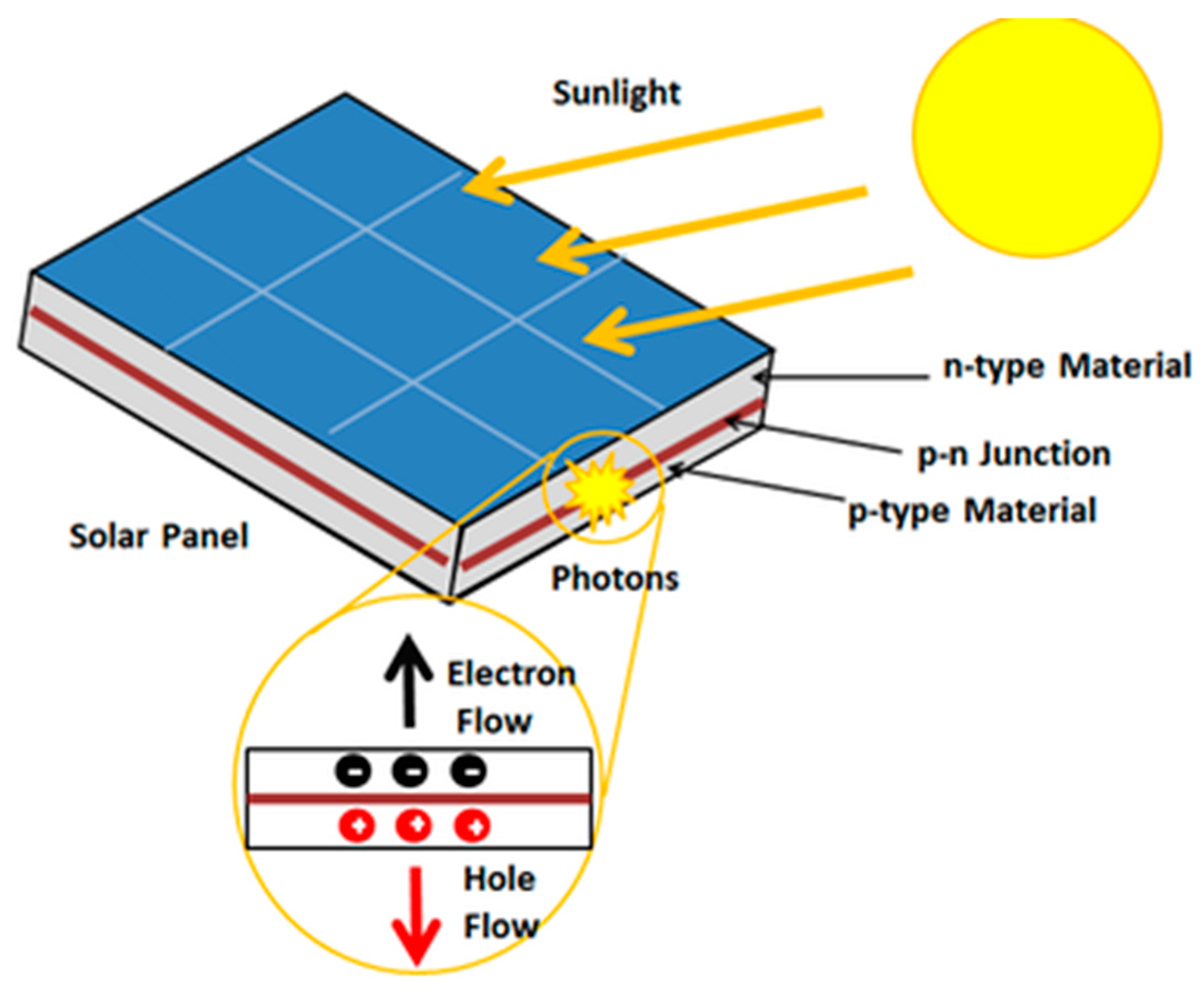
P-N junction diodes are utilized in the structure of the PV module. As they are semiconductor devices, they can convert the energy that is taken in into usable electrical power. These diodes can convert incident light into electrical energy when it reaches their surface. Figure 2 depicts the basic construction, connections, and functionality of a PV module:

As seen in the image below, there exist two distinct layers of silicon: a negative N layer and a boron-doped positive P layer. The PV module clad with tempered glass captures solar energy when subjected to sunlight. The energy collected eventually rises above the band gap energy level, causing electrons to pass across that band on their way from the conduction band to the valence band. The conduction band’s electrons can therefore move freely and create electron–hole pairs. The electricity generated during the process is used to power the load because the motion of electrons is what causes the passage of electric current. An array configuration is not sufficient to produce enough electricity because it suffers from multiple losses. The maximum power point tracking (MPPT) technique is the best way to maximize each string’s efficiency. By employing such control strategies, PV modules can produce the maximum amount of electricity achievable.

4. Methodology

Feature analysis and classification using Gaussian radial Boltzmann with Markov encoder model:

The weighted sum of the densities of the M component parts is known as the mixture density. The ith component density is denoted by the expression $s(x;\theta i)$, where θ_i stands for the component parameters. With the restrictions that ${\pi }_i\ge 0$ and ${\sum }_{i=1}^M{\pi }_i=1$, we use π_i to signify the weighting factor or “mixing proportions” of the i^th component in combination. The chance that a data sample belongs to the ith mixture component is represented by s(i), and M _i = 1. Equations (15) and (16) are then used to define an M component mixture density (16),

$$s(x)={\sum }_{i=1}^M{\pi }_{i}p\left(x;{\theta }_i\right),i=1,\dots ,M$$

(15)

$$s(\mathrm{x})={\sum }_{c=1}^c{\pi }_c{f}_c(\mathrm{x}\mid \theta )$$

(16)

The mixture model has a vector of parameters, $\underset{\_}{\theta }=\left\{{\theta }_1,\dots ,{\theta }_M,{\pi }_1,\dots {\pi }_M\right\}$

Hidden variables are treated as a latent variable, or z, in mixture models. It accepts values 1 through M as a discrete set that satisfies the conditions $z_Mϵ\left\{\mathrm{0,1}\right\}$ and ${\sum }_M{z}_M=1$. A conditional distribution p(x|z) and a marginal distribution p(z) are how we define the joint distribution p(x, z), i.e., from Equation (17),

$$p(z,x)=p\left(z\right)p(x\mid z)$$

(17)

Mixing coefficients k are used to specify the marginal distribution across z, as illustrated in Equation (18),

$$p\left(z_k=1\right)={\pi }_k$$

(18)

Equations (19) and (20) define probability density function of X.

$$p\left(x\mid {\mu }_k,{\mathsf{\Sigma }}_k\right)=\frac{1}{\sqrt{2\pi \left|{\mathsf{\Sigma }}^{-1}\right|}}\mathrm{e}\mathrm{x}\mathrm{p}\left(-\frac{1}{2}\left(x-{\mu }_x\right){\mathsf{\Sigma }}_x^{-1}{\left(x-{\mu }_x\right)}^T\right)$$

(19)

$$f_c\left(\mathrm{x}\mid {\mu }_c,{\mathsf{\Sigma }}_c\right)=\frac{1}{{(2\pi )}^{\frac{1}{t}}{\left|{\mathsf{\Sigma }}_c\right|}^{\frac{1}{2}}}\mathrm{e}\mathrm{x}\mathrm{p}\left(-\frac{1}{2}{\left(\mathrm{x}-{\mu }_c\right)}^t{\mathsf{\Sigma }}_c^{-1}\left(\mathrm{x}-{\mu }_c\right)\right)$$

(20)

where ${\mu }_x$ is an $\left({\mu }_{x1},\dots ,{\mu }_{xN}\right)$ and ${\mathsf{\Sigma }}_x$ covariance matrix and ${\mathsf{\Sigma }}_x$ is a vector of means (_x1,..., _xN). Equations (21)–(23), which are linear superpositions of Gaussians, can be used to represent Gaussian mixture distribution.

$$p\left(x\right)={\sum }_{k=1}^K{\pi }_{k}p\left(x\mid {\mu }_k,{\mathsf{\Sigma }}_k\right)$$

(21)

$$\begin{gathered} {\widehat{\pi }}_c=\frac{n_c}{n}, \\ {\dot{\mu }}_c=\frac{1}{n_c}{\sum }_{\left(i,y_i=c_j\right)}{\mathrm{x}}_i,p\left(x\mid z_k=1\right)=p\left(x\mid {\mu }_k,{\mathsf{\Sigma }}_k\right), \\ {\stackrel{\mathrm{ˆ}}{\mathsf{\Sigma }}}_c=\frac{1}{\left(n_c-1\right)}{\sum }_{\left(i\mid y_i=c\right)}\left({\mathbf{x}}_i-{\mu }_c\right){\left({\mathbf{x}}_i-{\mu }_c\right)}^t \end{gathered}$$

(22)

Conditional distribution of x for a specific value of z is a Gaussian, according to Equation (23):

$$p(x\mid z)={\prod }_{k=1}^{K}p{\left(x\mid {\mu }_k,{\mathsf{\Sigma }}_k\right)}^{z_k}$$

(23)

By adding joint distribution of all possible states of z to obtain Equation (24), one may determine the marginal distribution of x.

$$p(x)={\sum }_{z}p\left(z\right)p(x\mid z)={\sum }_{k=1}^K{\pi }_{k}p\left(x\mid {\mu }_k,{\mathsf{\Sigma }}_k\right)$$

(24)

The “posterior probability” on a mixture component for a specific data vector is a significant derived quantity and is indicated in Equation (25):

$$\gamma \left(z_{nk}\right)=\frac{{\pi }_{k}N\left(x_n\mid {\mu }_k,{\mathsf{\Sigma }}_k\right)}{{\sum }_{j=1}^K{\pi }_{j}N\left(x_n\mid {\mu }_j,{\mathsf{\Sigma }}_j\right)}=\frac{p\left(z_k=1\right)p\left(x\mid z_k=1\right)}{{\sum }_{j=1}^{K}p\left(z_j=1\right)p\left(x\mid z_j=1\right)}$$

(25)

Maximal likelihood is the learning objective of RBMs, which are energy-based approaches. Equation (26), in its combined structure, defines the energy of its hidden parameters (e) and visible parameters (f).

$$En(\mathrm{e},\mathrm{f};\theta )=-{\sum }_{ij}{\mathrm{W}}_{ij}{\mathrm{f}}_i{\mathrm{e}}_j-{\sum }_i{\mathrm{b}}_i{\mathrm{f}}_i-{\sum }_j{\mathrm{a}}_j{\mathrm{e}}_j.$$

(26)

θ represents the element W(a, b). Using Equation (27), one can determine the combined probability of v and h.

$$P_{\theta }(\mathrm{f},\mathrm{e})=\frac{1}{Z\left(\theta \right)}\mathrm{e}\mathrm{x}\mathrm{p}(-En(\mathrm{f},\mathrm{e};\theta )).$$

(27)

In this context, the partition function is denoted by Z(θ). The previous equation can be rewritten as Equation (28).

$$P_{\theta }(\mathrm{f},\mathrm{e})=\frac{1}{Z\left(\theta \right)}\mathrm{e}\mathrm{x}\mathrm{p}\left({\sum }_{i=1}^D{\sum }_{j=1}^F{\mathrm{W}}_{ij}{\mathrm{f}}_i{\mathrm{e}}_j+{\sum }_{i=1}^D{\mathrm{f}}_i{\mathrm{b}}_i+{\sum }_{j=1}^F{\mathrm{e}}_j{\mathrm{a}}_j\right)$$

(28)

Maximizing the probability function P(f) is the goal. The edge distribution of P(f, e) makes it easy to calculate P(f) by Equation (29):

$$P_{\theta }(\mathrm{f})=\frac{1}{Z\left(\theta \right)}{\sum }_{\mathrm{h}}\mathrm{e}\mathrm{x}\mathrm{p}\left[{\mathrm{f}}^T\mathrm{W}\mathrm{h}+{\mathrm{a}}^T\mathrm{h}+{\mathrm{b}}^T\mathrm{f}\right]$$

(29)

The RBM parameters are derived (f) by optimizing P. By optimizing log(P(f)) = L(), we can obtain maximum P(f) using Equation (30):

$$\begin{array}{c}L(\theta )=\frac{1}{N}{\sum }_{n=1}^N\mathrm{l}\mathrm{o}\mathrm{g}{P}_{\theta }\left({\mathrm{f}}^{\left(n\right)}\right)\hfill \\ \begin{array}{cc}\hfill \frac{\partial L\left(\theta \right)}{\partial {\mathrm{W}}_{ij}}=\frac{1}{N}{\sum }_{n=1}^N& \frac{\partial }{\partial W_{ij}}\mathrm{l}\mathrm{o}\mathrm{g}\left({\sum }_{\mathrm{h}}\mathrm{e}\mathrm{x}\mathrm{p}\left[{\mathrm{f}}^{\left(n\right)T}\mathrm{W}\mathrm{h}+{\mathrm{a}}^T\mathrm{h}+{\mathrm{b}}^T{\mathrm{f}}^{\left(n\right)}\right]\right)\hfill \\ \hfill -& \frac{\partial }{\partial W_{ij}}\mathrm{l}\mathrm{o}\mathrm{g}Z(\theta )=E_{P_{\mathrm{dut}}}\left[{\mathrm{f}}_i{\mathrm{e}}_j\right]-E_{P_{\theta }}\left[{\mathrm{f}}_i{\mathrm{e}}_j\right]\hfill \end{array}\end{array}$$

(30)

The original purpose of stochastic gradient descent was to maximize L(θ). Next, Equation (30) is used to calculate the L(θ) derivative for W.

The formula’s first part is easy to evaluate. Across all datasets, the values of fi and ej are averaged. It is computationally challenging to solve the remaining part of the equation, which comprises all 2|f|+|e| possible values of f and e. The formula’s second part is Equation (31).

$${\sum }_{f,e}{\mathrm{f}}_i{\mathrm{e}}_j{P}_{\theta }(\mathrm{f},\mathrm{e})$$

(31)

Monte Carlo simulations are used to estimate gradient as shown in the following equation:

$$\begin{gathered} \Delta {\mathrm{a}}_i=f_i^{\left(0\right)}-f_i^{\left(k\right)} \\ \Delta {\mathrm{b}}_i=P\left({\mathrm{e}}_j=1\mid {\mathrm{f}}^{\left(0\right)}\right)-P\left({\mathrm{e}}_j=1\mid {\mathrm{f}}^{\left(k\right)}\right) \\ \Delta {\mathrm{W}}_{ij}=P\left({\mathrm{e}}_j=1\mid {\mathrm{f}}^{\left(0\right)}\right){\mathrm{f}}_i^{\left(0\right)}-P\left({\mathrm{e}}_j=1\mid {\mathrm{f}}^{\left(k\right)}\right){\mathrm{f}}_i^{\left(k\right)} \end{gathered}$$

(32)

where f(0) I is sample value and f(k) I is a sample that satisfies distribution P(f) identified by sampling. Lastly, Equation (33) provides the parameter update equation.

$$\begin{array}{c}{\mathrm{a}}_i={\mathrm{a}}_i+\Delta {\mathrm{a}}_i\hfill \\ {\mathrm{b}}_j={\mathrm{b}}_j+\Delta {\mathrm{b}}_j\hfill \\ {\mathrm{W}}_{ij}={\mathrm{W}}_{ij}+\Delta {\mathrm{W}}_{ij}\hfill \end{array}$$

(33)

The probability distribution is shown below by Equation (34).

$$\begin{gathered} P\left(V,e^{\left(1\right)},e^{\left(2\right)}\right)=\frac{1}{\mathrm{Z}\left(\theta \right)}\mathrm{e}\mathrm{x}\mathrm{p}-E\left(V,e^{\left(0\right)},e^{\left(\mathsf{\Omega }\right)};\theta \right) \\ \mid P\left(V,e^{\left(1\right)},e^{\left(2\right)}\right)=-V^T{W}^{\left(1\right)}{e}^{\left(1\right)}-V^T{W}^{\left(2\right)}{e}^{\left(2\right)}+b \end{gathered}$$

(34)

Encoders and decoders are essential elements of its design. Encoder and decoder both implement standard matrix multiplication. As a normalizing function, an encoder gradient function is utilized. After adjusting the weight and biases of the autoencoder, Equation (35) operates network training.

$$e^{\left(0\right)}=a\left(b^{\left(n\right)}+V^T{W}^{\left(n\right)}\right)$$

(35)

$$e^{\left(n\right)}=\sigma \left(b_i^{\left(n\right)}+e^{(n-1)T}{W}^{\left(n\right)}\right)$$

where $n=\mathrm{1,2},3,\dots ,m$.

Consider training an HSI datacube with two hidden layers using Equations (36) and (37).

$$P\left(V_i=1;e^{\left(2\right)},e^{\left(2\right)}\right)=\alpha V^T{W}_1^{\left(1\right)}+\alpha V^T{W}_1^{\left(2\right)}$$

(36)

When n = 1:

$$\begin{gathered} P\left(V_i=1;e^{\left(1\right)},e^{\left(2\right)}\right)=\alpha V^T{W}_1^{\left(1\right)}+\alpha V^T{W}_i^{\left(2\right)} \\ P\left(V_i=2;e^{\left(1\right)},e^{\left(2\right)}\right)=a{V}^T{W}_2^{\left(1\right)}+a{V}^T{W}_2^{\left(2\right)} \end{gathered}$$

(37)

Mean-field value is represented by Equation (38):

$$P(x)={\sum }_{h=\mathrm{1,2}}Q\left(e^{\left(1\right)},e^{\left(2\right)}\right)\mathrm{l}\mathrm{o}\mathrm{g}\left(\frac{e^{\left(i\right)},e^{\left(2\right)}}{P\left(e^{\left(1\right)},e^{\left(2\right)}\right)}\right)$$

(38)

where Gibbs energy is represented by Equation (39):

$$E(x)=\frac{1}{Z\left(D\right)}\mathrm{e}\mathrm{x}\mathrm{p}(-P(x))$$

(39)

By indicating a weight change, (40) and (41) present a new weight value. Each stratum is assigned the b = 0 bias.

$$\Delta e_i^{\left(1\right)}=\alpha {\sum }_i{V}_i{W}^{\left(1\right)}$$

(40)

$$\Delta e_i^{\left(2\right)}=\alpha {\sum }_i{V}_i{W}^{\left(2\right)}$$

(41)

Convolution filters and the weights of fully connected layers are two model parameters that are optimized using the gradient descent approach. It is essential to classify the image into the correct category since the final layer has a significant impact on classification outcomes. This is carried out by properly linking the weights from the prior layers. Here, in order to improve classification accuracy, the training of the final weight vector is optimized utilizing a newly created modified whale optimization method. The number of search agents is limited to 50, the utmost number of iterations is limited to 100, and the final parameter (vector a) is linearly modified between [0,2].

5. Performance Analysis

To computationally evaluate the cloud DNSE algorithm, the simulation set contains sensitivity based on error in measurement, grid variables, DNSE efficiency, and pseudo measurements. Reading the voltages at the node from a smart meter is the initial stage in this endeavor since smart meters are not set up to determine the voltages in the LV grid under examination. If the powers and voltages at all nodes are being monitored concurrently, this phase can be avoided.

Table 1. Distributed Networks of LV Grid.

Distributed Networks	$\mathbf{Resistance} \mathsf{\Omega }/\mathbf{k}\mathbf{m}$	$\mathbf{Series} \mathbf{Reactance} \mathsf{\Omega }/\mathbf{k}\mathbf{m}$	$\mathbf{Shunt} \mathbf{Admittance} \mathsf{\mu }\mathbf{S}/\mathbf{k}\mathbf{m}$
Type 1	0.207	0.072	204.2
Type 2	0.320	0.075	175.9
Type 3	0.727	0.087	125.6

displays dispersed networks for the low-voltage grid’s resistance, reactance, and admittance by both series and shunt in accordance with their network types.

Table 2. Analysis based on various circuit models.

Circuit Model	Techniques	Power Analysis	Energy Efficiency	QoS	Accuracy	Precision	Recall
Resistance	EMS	79	88	66	81	77	66
	LSTM	81	89	68	83	79	68
	Proposed method	83	92	71	85	81	72
Reactance	EMS	82	89	69	82	79	69
	LSTM	85	93	72	84	82	73
	Proposed method	87	95	75	86	83	75
Admittance network type	EMS	84	91	75	85	81	72
	LSTM	86	93	76	91	83	75
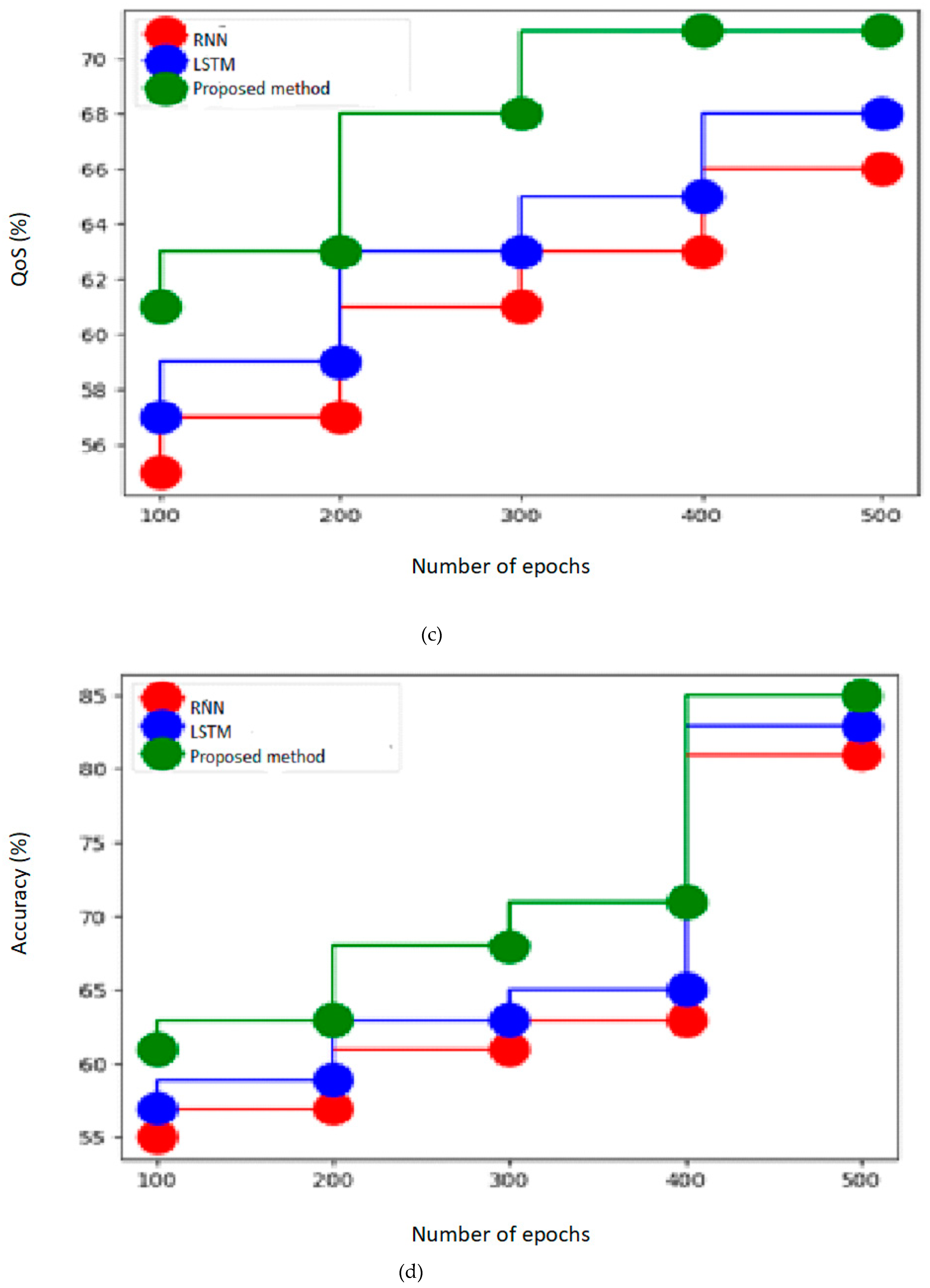
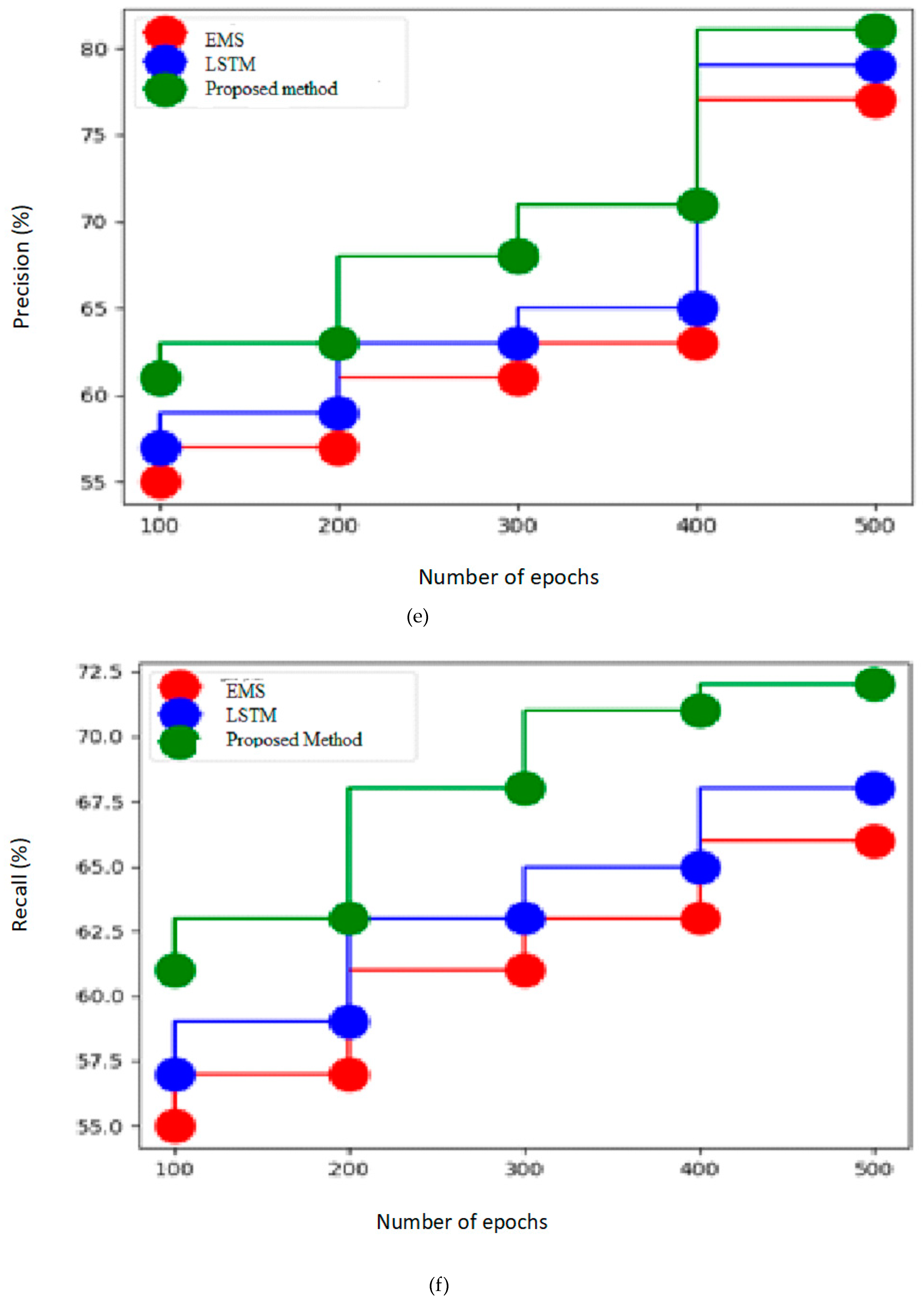
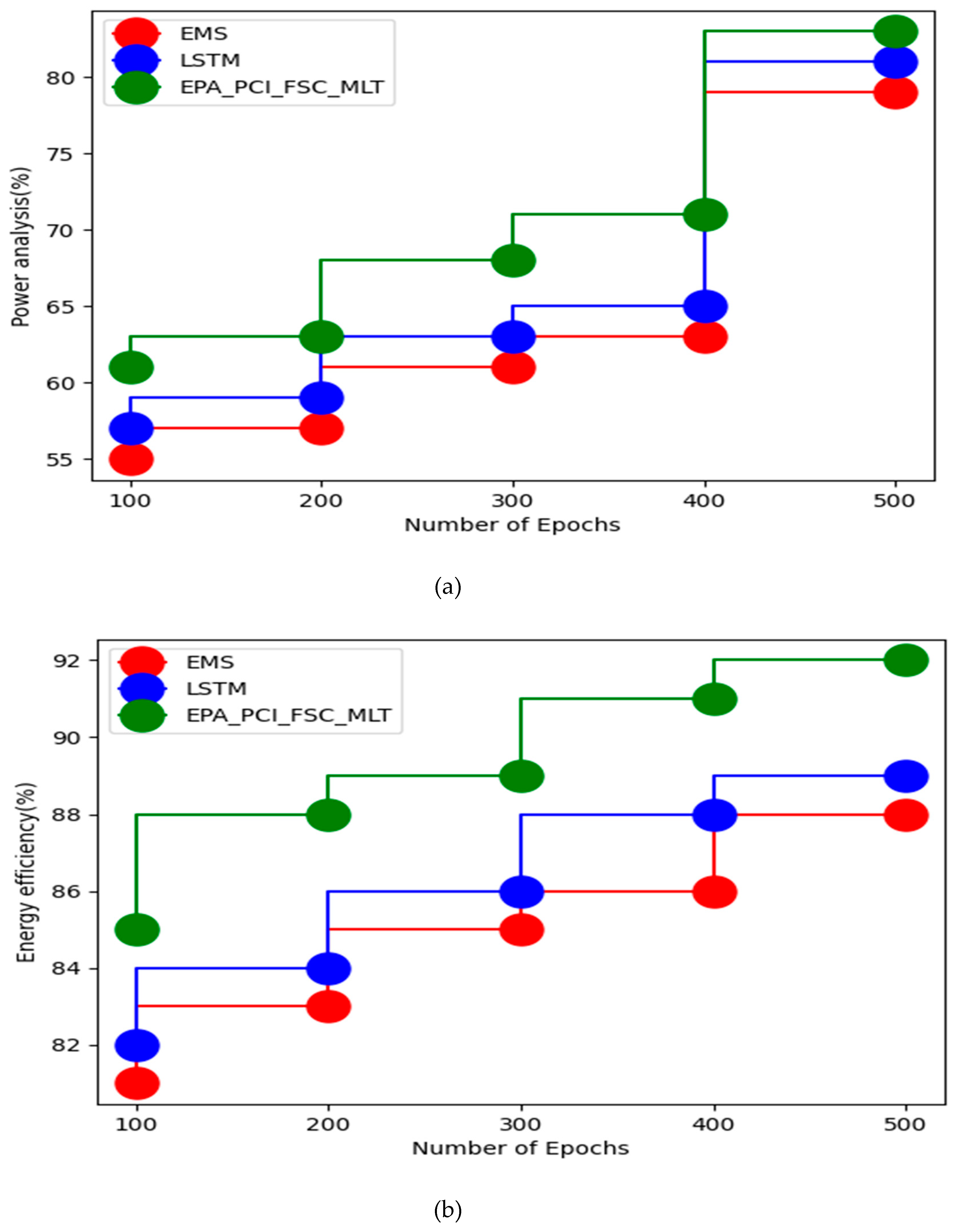
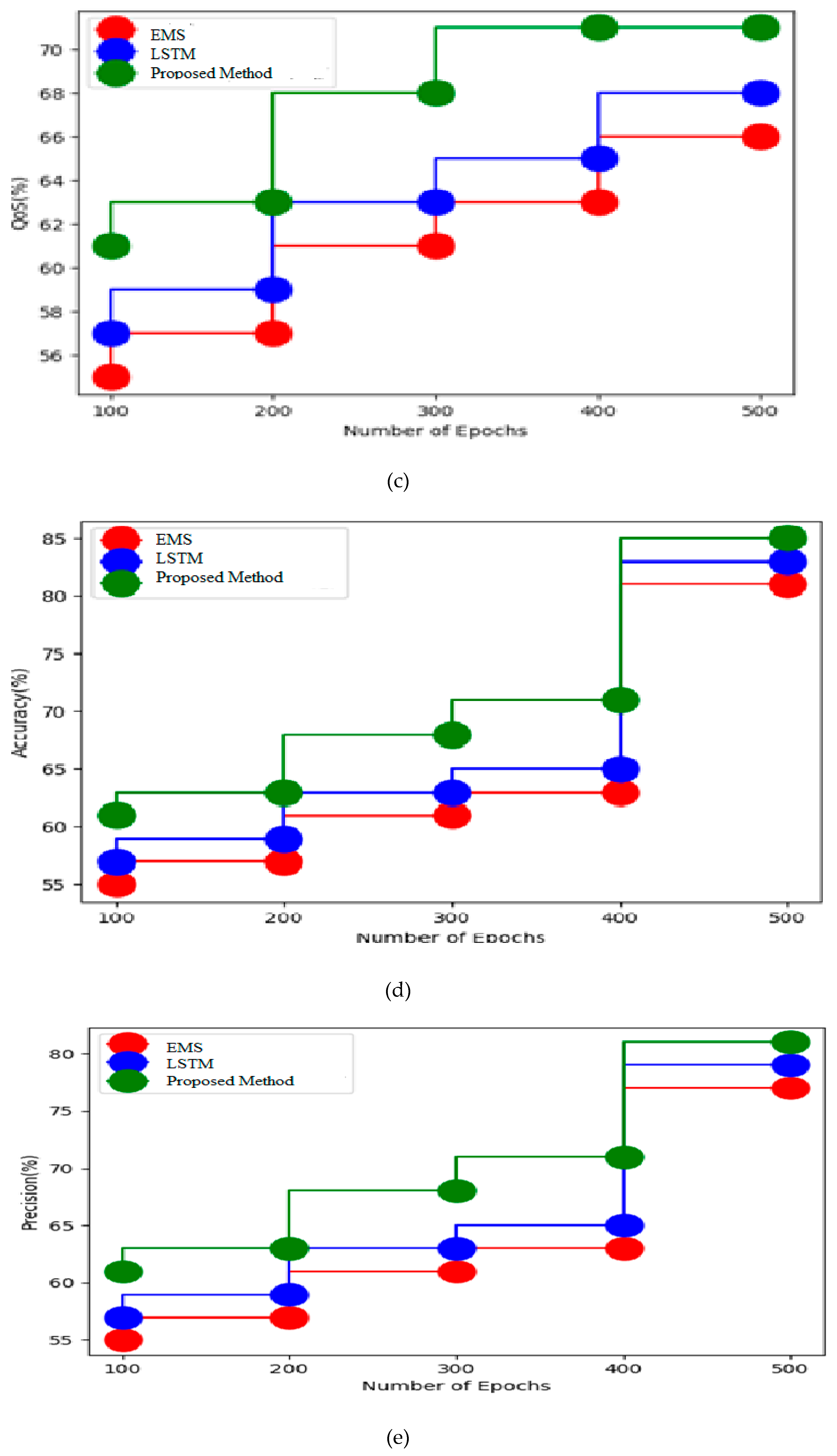
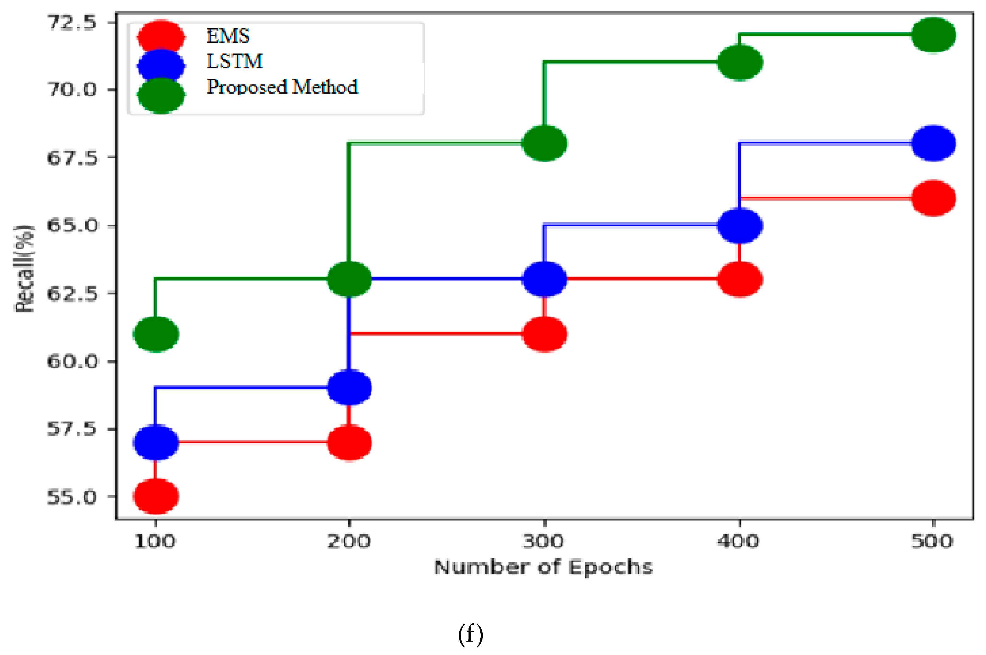
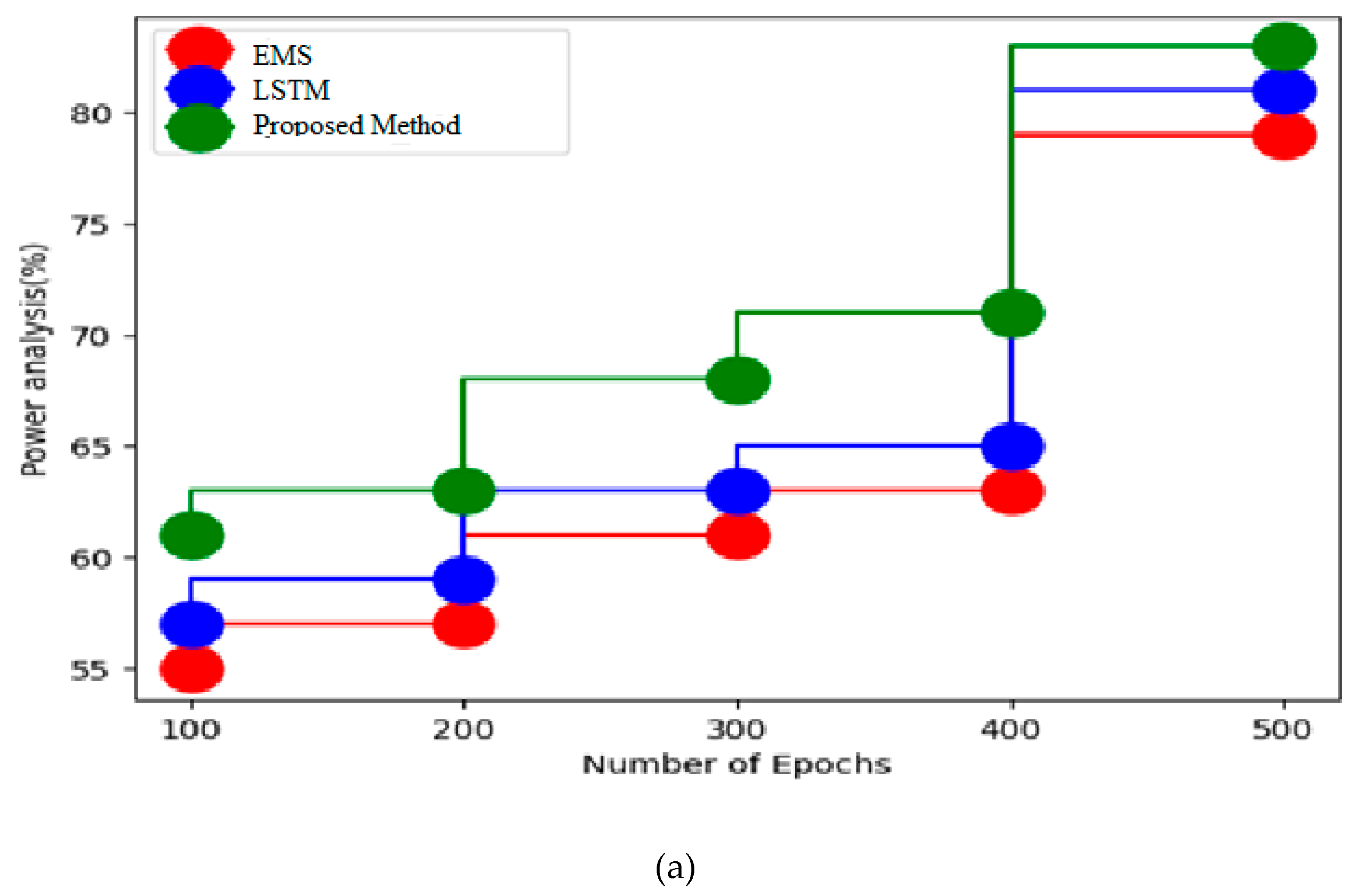
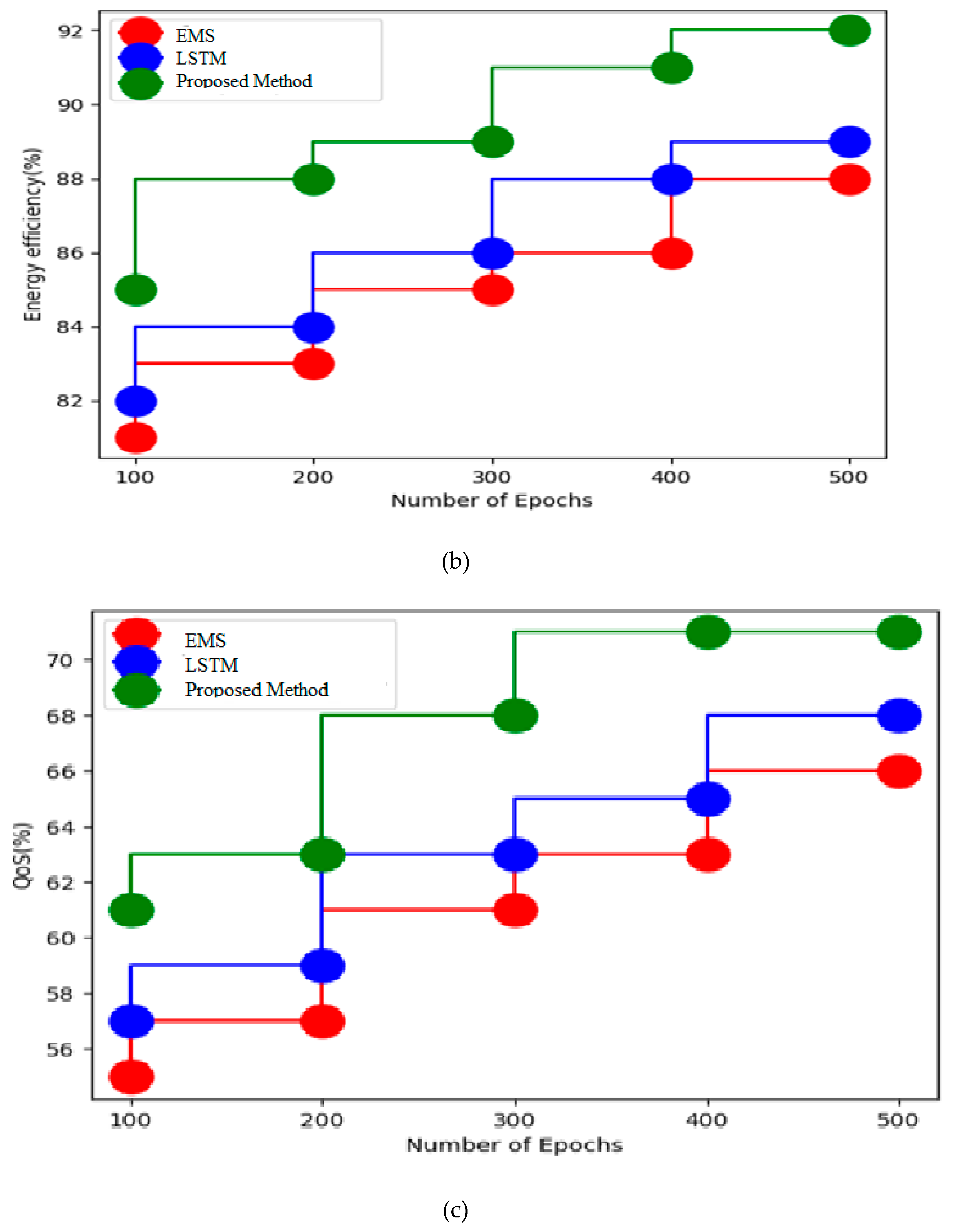
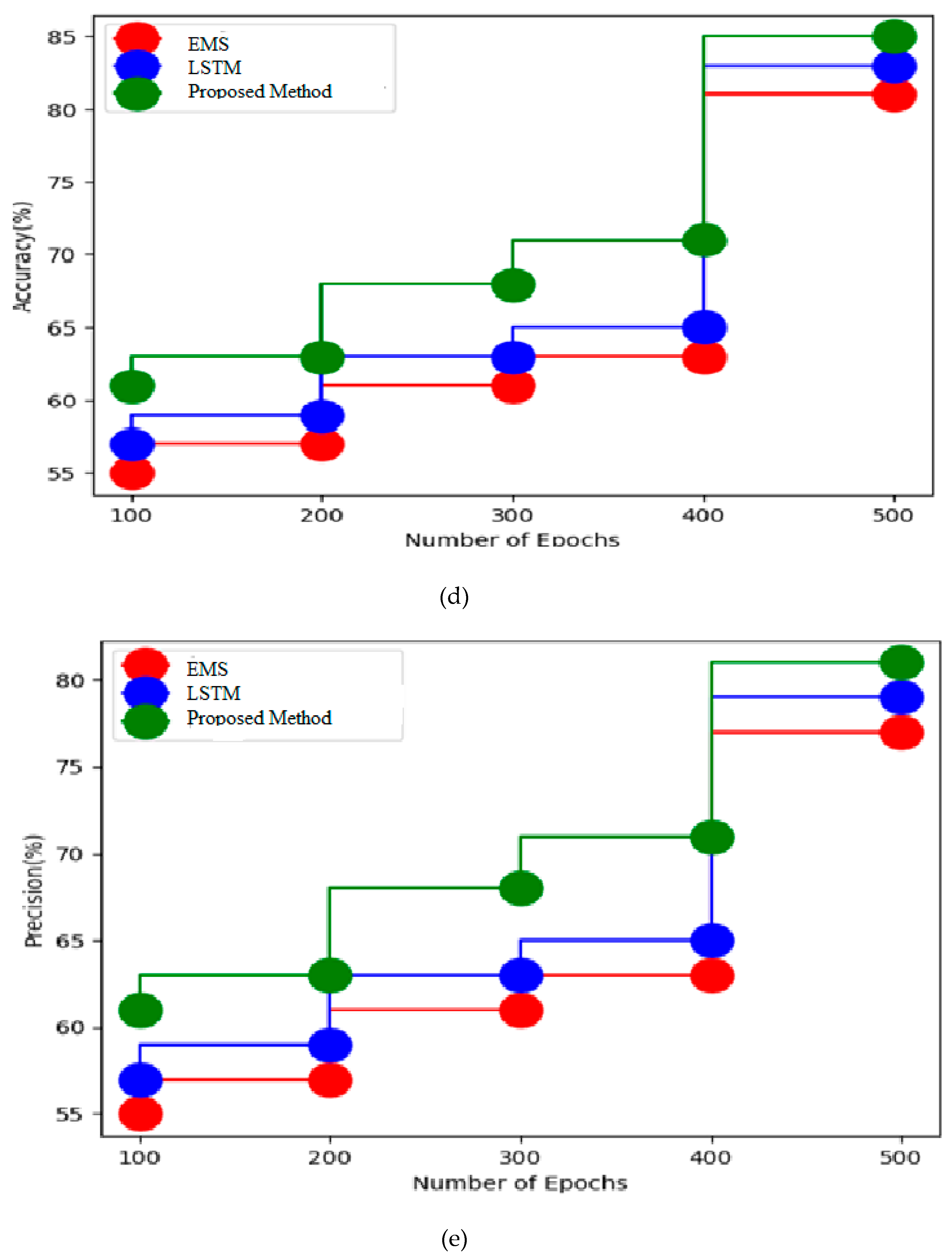
	Proposed method	88	95	77	93	85	77

gives analysis based on various circuit models. The circuit models analyzed are resistance, reactance and admittance network type in terms of power analysis, energy efficiency, QoS, accuracy, precision, and recall. The energy management system (EMS) and long short-term memory (LSTM) networks are compared.

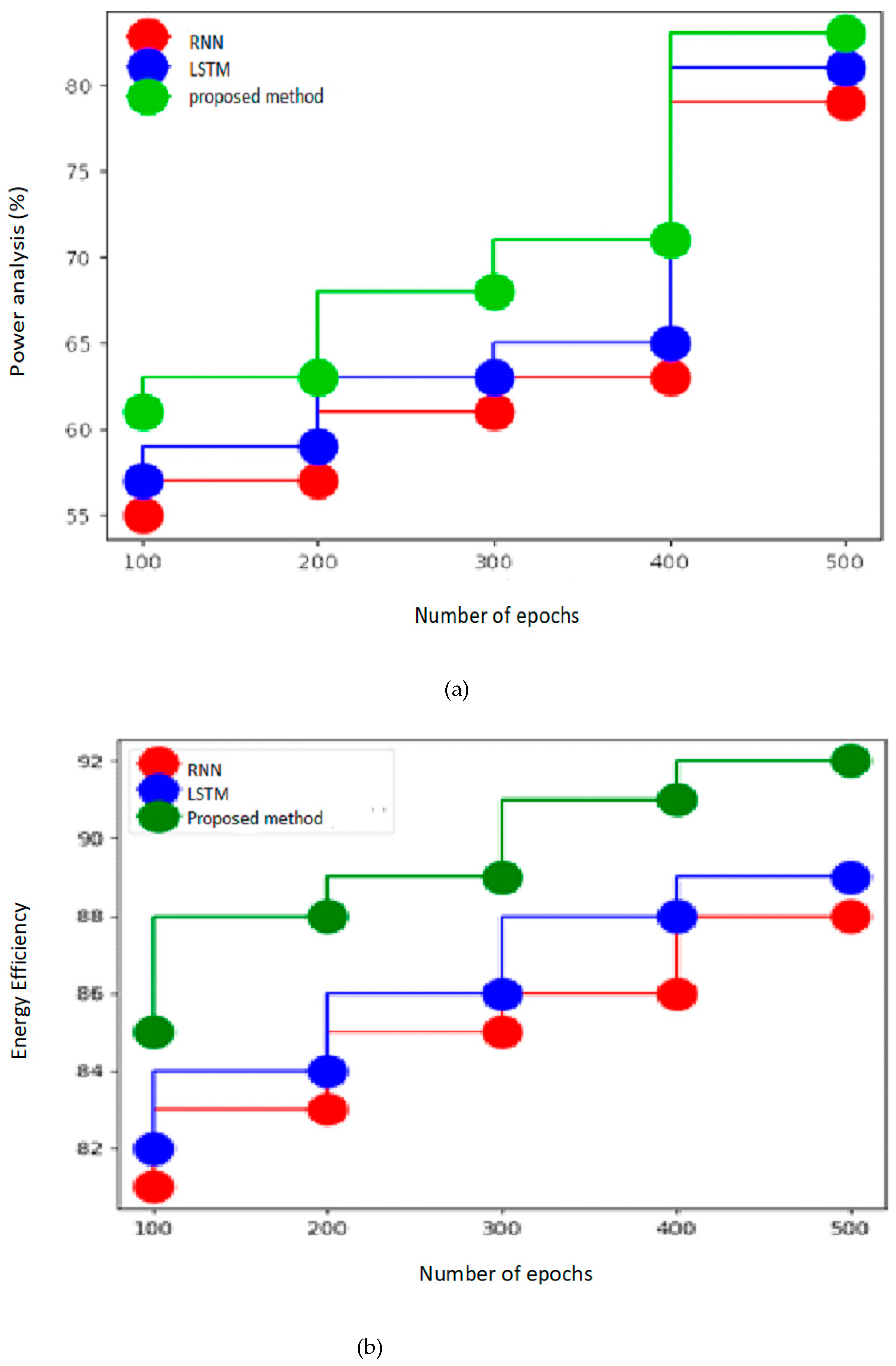
Figure 3a–f give analysis based on resistance type circuit model. The proposed technique attained power analysis of 83%, energy efficiency of 92%, QoS of 71%, accuracy of 85%, precision of 81%, and recall of 72%, EMS achieved a 79% power analysis, an 88% energy efficiency, a 66% quality of service, an 81% accuracy, a 77% precision, and a 66% recall, and power analysis of 83%, energy efficiency of 92%, QoS of 71%, accuracy of 85%, and precision of 81% were all achieved with LSTM.

Figure 4a–f show analysis for reactance circuit model. The proposed technique attained power analysis of 87%, energy efficiency of 95%, QoS of 75%, accuracy of 86%, precision of 83%, and recall of 75%, EMS achieved a power analysis of 82%, an energy efficiency of 89%, a QoS of 69%, an accuracy of 82%, a precision of 79%, and a recall of 69%, and 85% power analysis, 93% energy efficiency, 72% QoS, 82% accuracy, 81% precision, and 72% recall were achieved by LSTM.

Figure 5a–f give analysis based on admittance network type circuit model. Power analysis of 88%, energy efficiency of 95%, QoS of 77%, accuracy of 93%, precision of 85%, recall of 77%, and QoS of 93% were achieved with the proposed technique. In comparison to LSTM, EMS achieved power analysis of 86%, energy efficiency of 93%, QoS of 76%, accuracy of 85%, precision of 81%, and recall of 72%. EMS also achieved energy efficiency of 91%, QoS of 75%, accuracy of 85%, and recall of 72%.

6. Conclusions

This study proposes an idea for energy analysis based on a microgrid photovoltaic system using a deep learning method. The energy optimization of the microgrid was carried out using a photovoltaic-based energy system with distributed power generation. The data analysis has been carried out for feature analysis and classification using a Gaussian radial Boltzmann with Markov encoder model. When taking into account an MG with photovoltaics (PVs), solar radiations abruptly increase in intensity during the day. That will boost MG production at a specific moment. Table 2 presents the comparative analysis of the proposed method with EMS and LSTM and it was shown to achieve higher power analysis, energy efficiency, QoS, accuracy, precision, and recall for different circuit models. In power analysis, the proposed method achieves 5% and 2.4% increases compared to EMS and LSTM models, respectively, for resistance models. Similarly, it has shown an increase of 6% and 2.3% and 4.7% and 2.3% for reactance and admittance circuit models.