
A New Hybrid Multi-Population GTO-BWO Approach for Parameter Estimation of Photovoltaic Cells and Modules

 , , ,
, , ,  ,
,  and
and 
Abstract
:1. Introduction
- A novel approach of hybrid multi-population GTO-BWO is proposed in this work.
- The classical and CEC-C06 2019 benchmark functions are utilized to test and assess the proposed technique’s performance.
- The proposed HGTO-BWO is implemented to determine the ungiven parameters of TDM and DDM equivalent circuits of PV cells/panels.
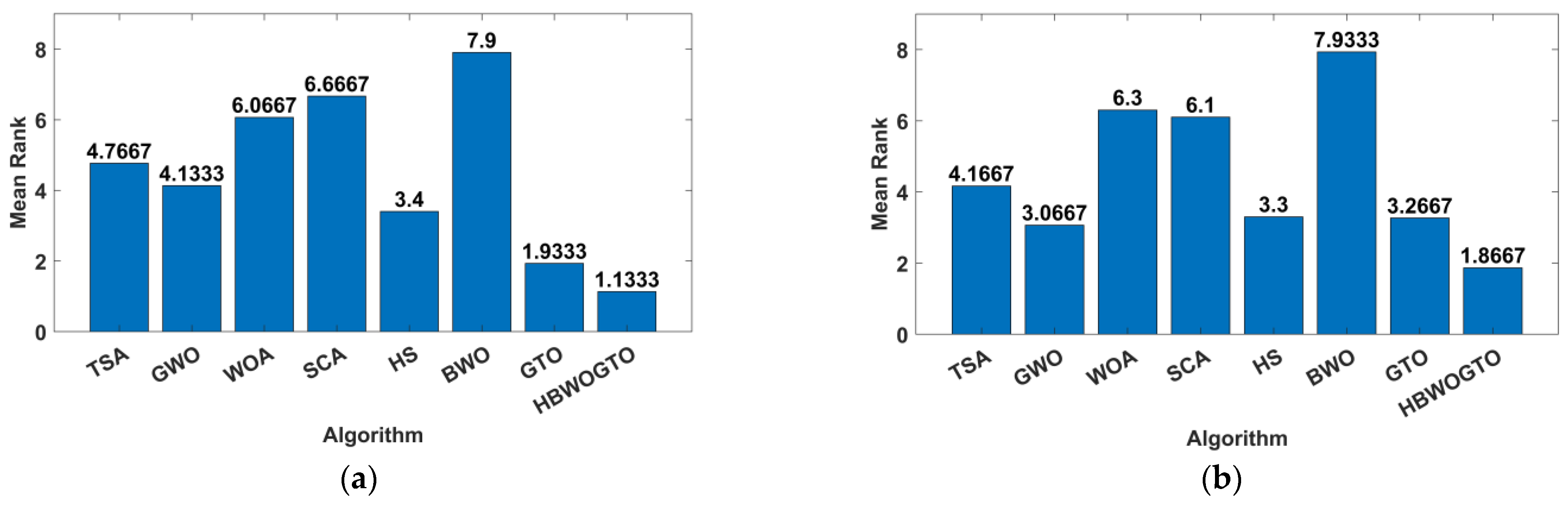
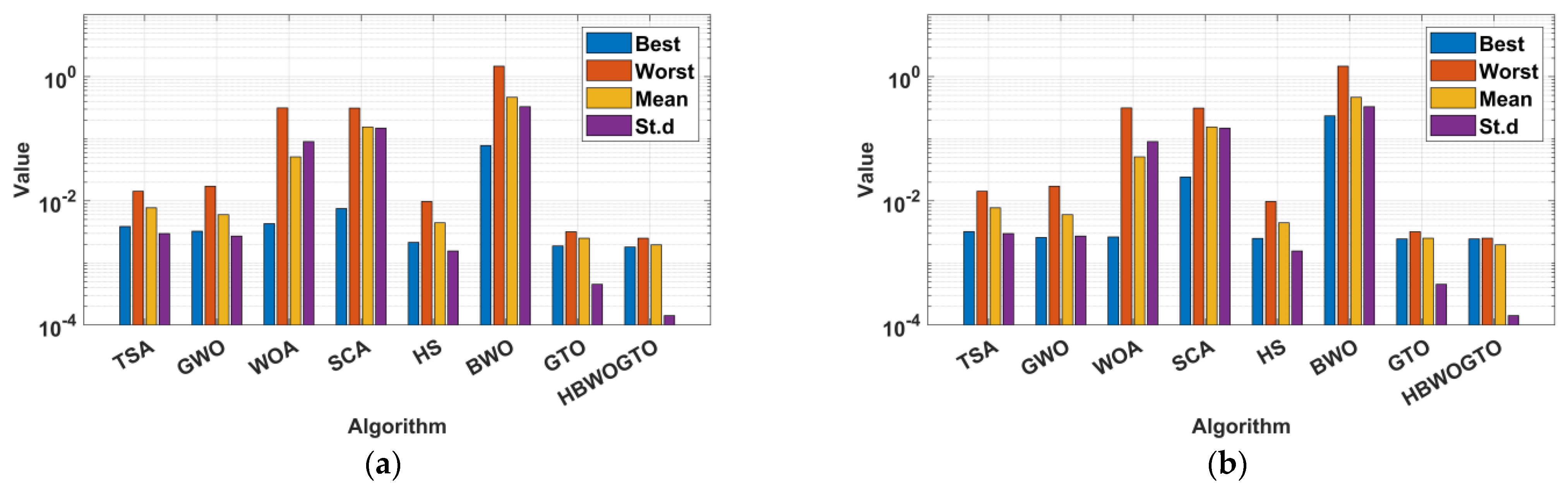
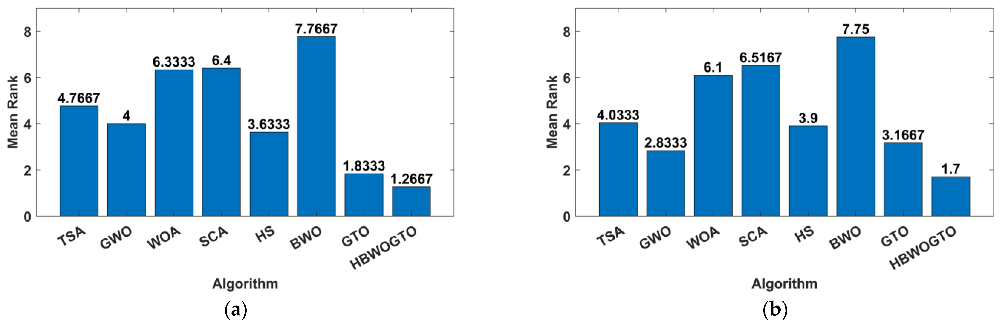
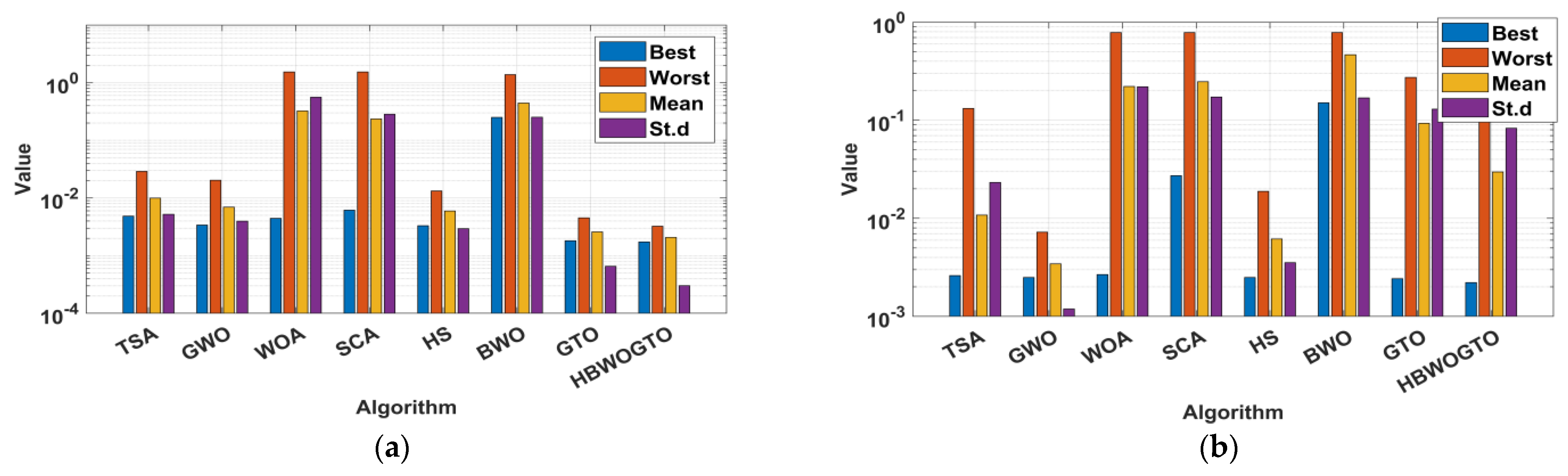
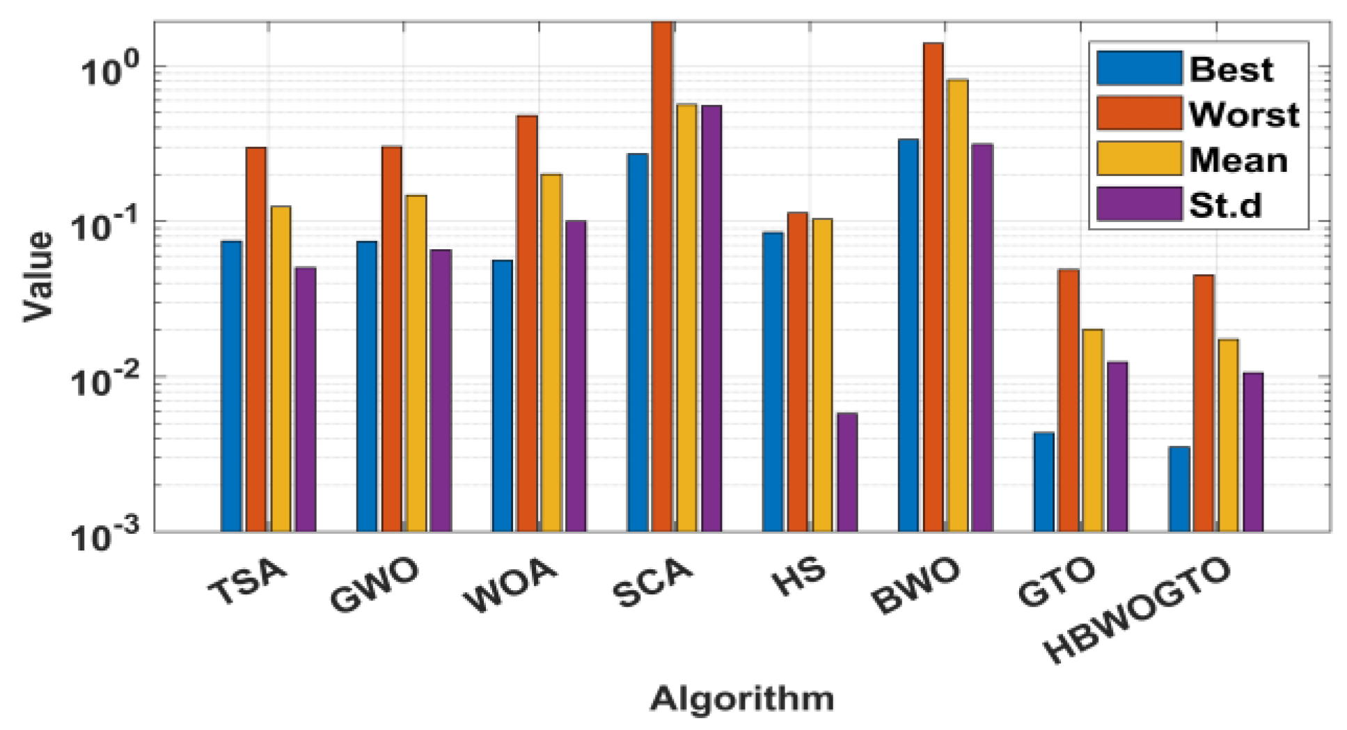
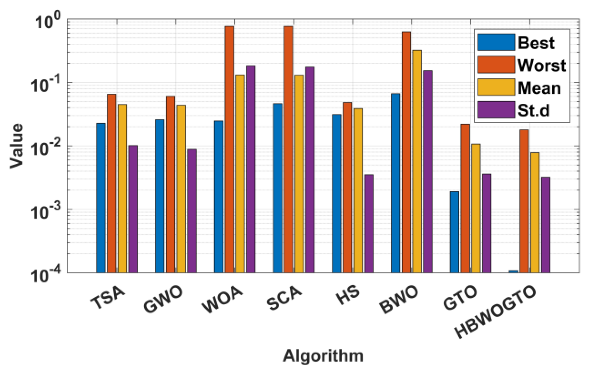
- A comparison is made with TSA, the grey wolf optimizer (GWO), the whale optimization algorithm (WOA), the sine cosine algorithm (SCA), harmony search (HS), beluga whale optimization (BWO), and the artificial gorilla troops optimizer (GTO).
- The fetched results assure the effectiveness and validity of the suggested HGTO-BWO.
2. Modeling of Solar Photovoltaic (PV)
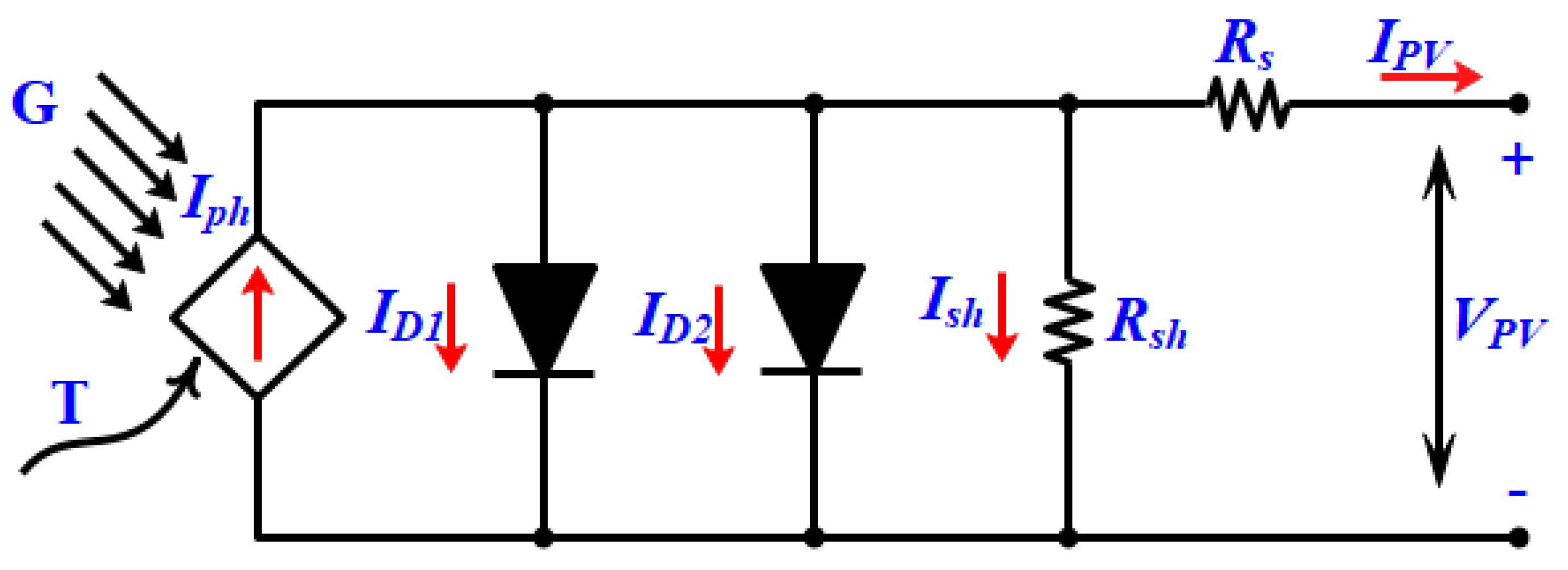
2.1. Double Diode Model (DDM)
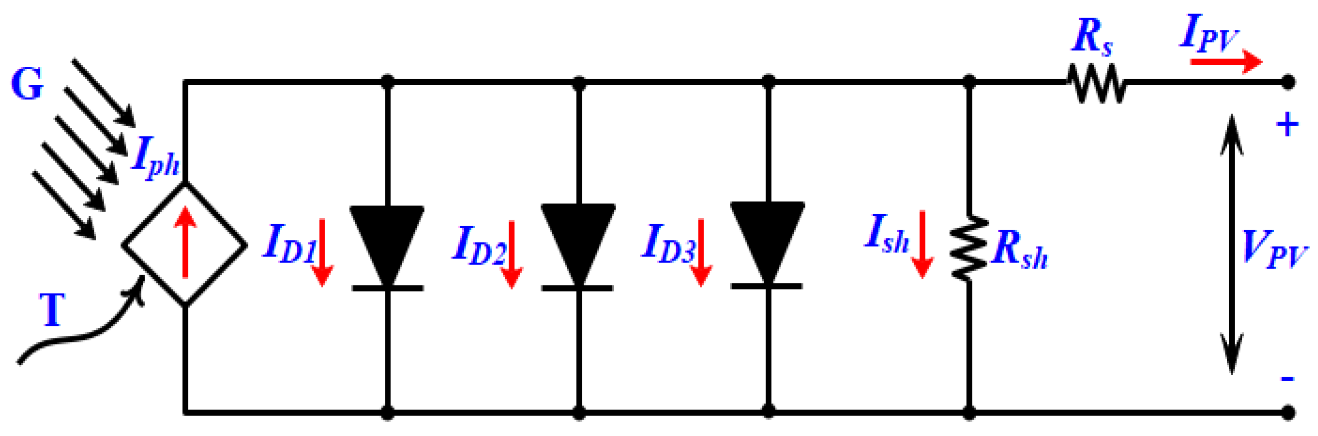
2.2. Triple Diode Model (TDM)
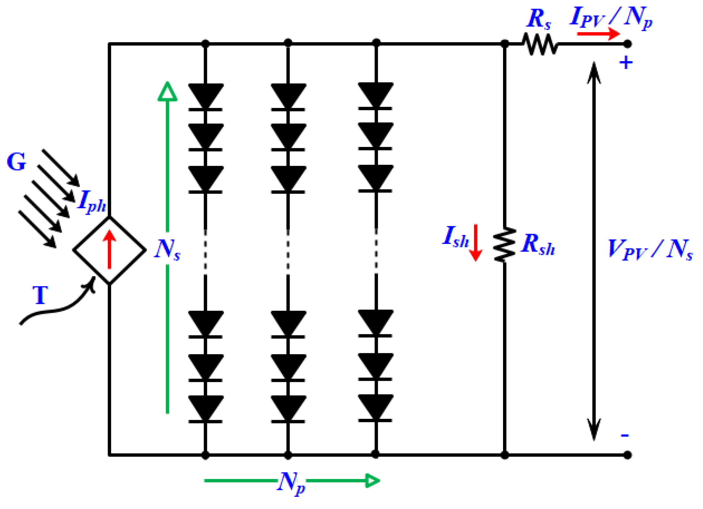
2.3. PV Panel Model
3. Problem Expression
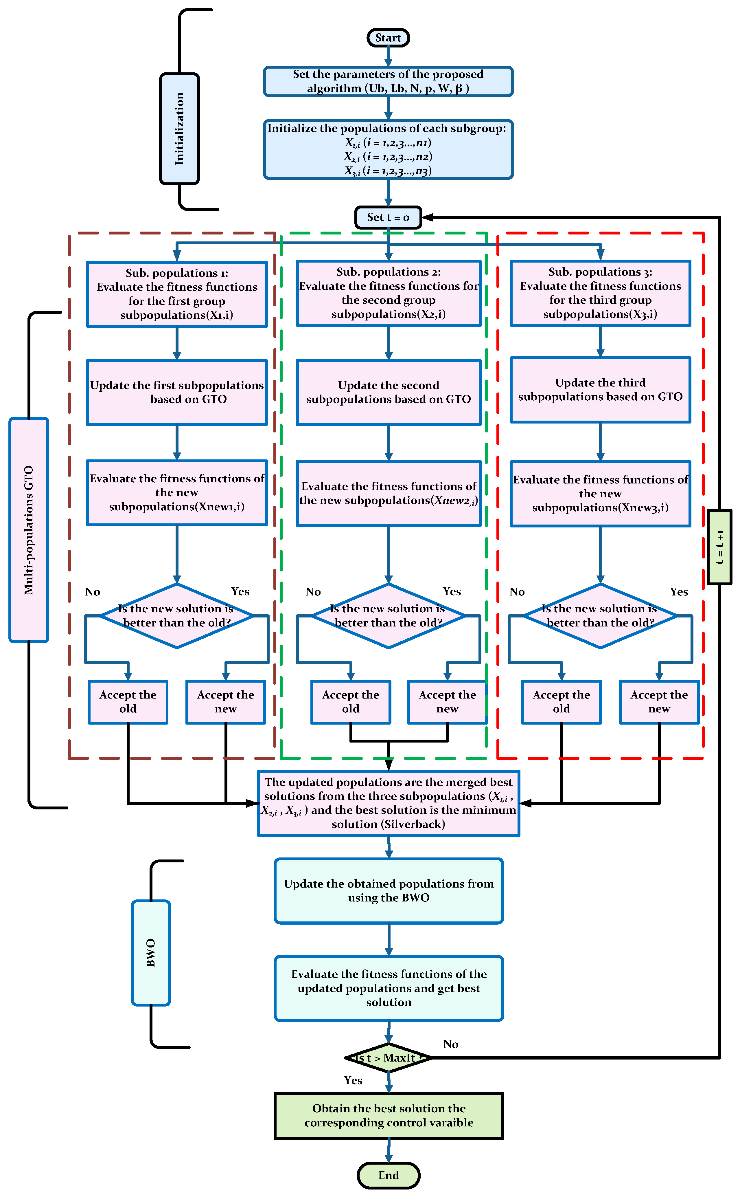
4. The Proposed Solution Methodology
4.1. Gorilla Troops Optimizer (GTO)
| Algorithm 1 The Pseudocode of GTO |
| Start GTO the corresponding fitness function. Initialize the populations and calculate the objective functions and assign the best result. using Equations (13) and (15). Update the positions of the gorillas according to (12). Compute the fitness function and assign the best solution. Update the positions of the gorillas using Equation (18). Otherwise Update the positions of the gorillas using Equation (21). end Calculate the objective functions for the new locations and include them, if their values are better than the previous solutions End while End GTO |
4.2. Beluga Whale Optimization (BWO)
| Algorithm 2 The Pseudocode of the BWO |
| Start BWO of the populations and the corresponding fitness function. Update the values of the using , and using Equations (27), (30) and (34). // Exploration phase Update the locations of the BWs using Equation (25). Otherwise // Exploitation phase Update the locations of the gorillas using Equation (26). end Compute the fitness functions for the new positions and select the best result. // whale fall Update the locations of the BWs using Equation (31). End Compute the fitness functions for the new positions and select the best result. End while End BWO |
4.3. The Proposed Hybrid Multi-Population GTO and BWO
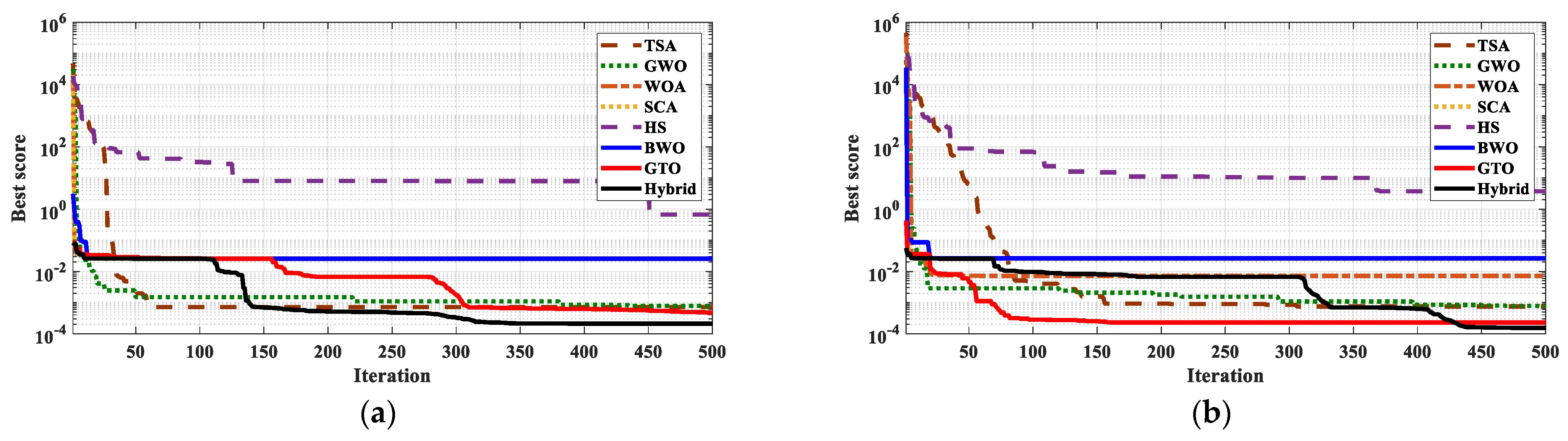
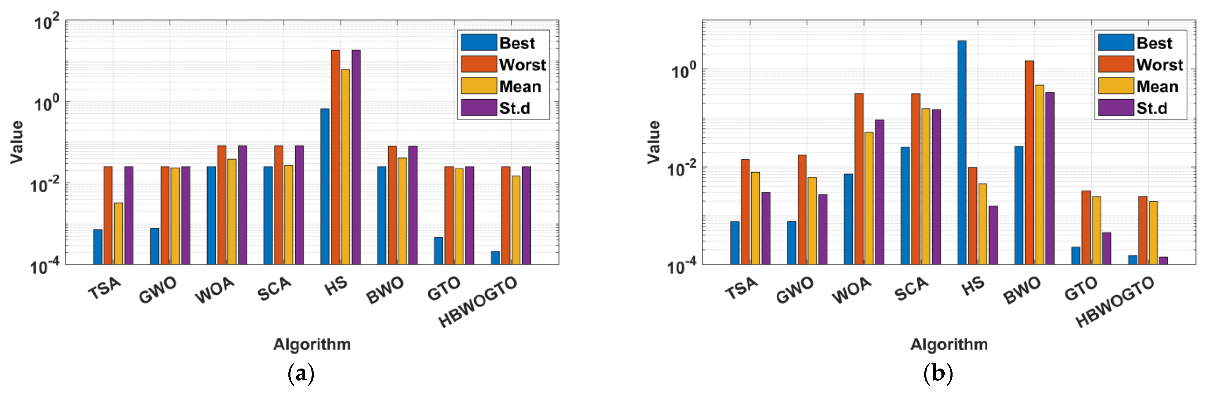
5. Testing of Benchmark Function
5.1. Traditional Benchmark Functions
5.2. CEC-C06 2019 Benchmark Functions
6. Application of HGTO-BWO: Parameter Estimation of PV Cell/Module
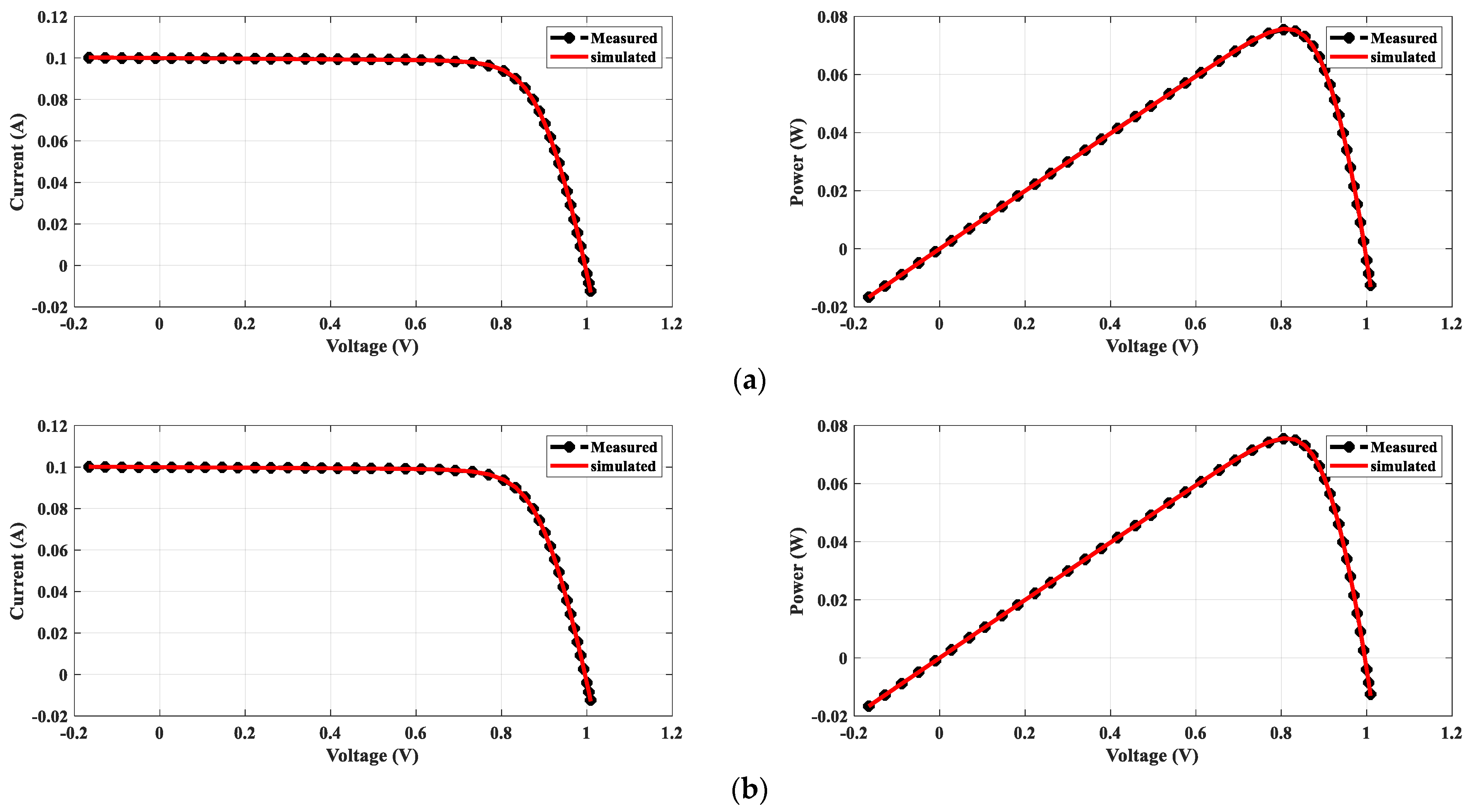
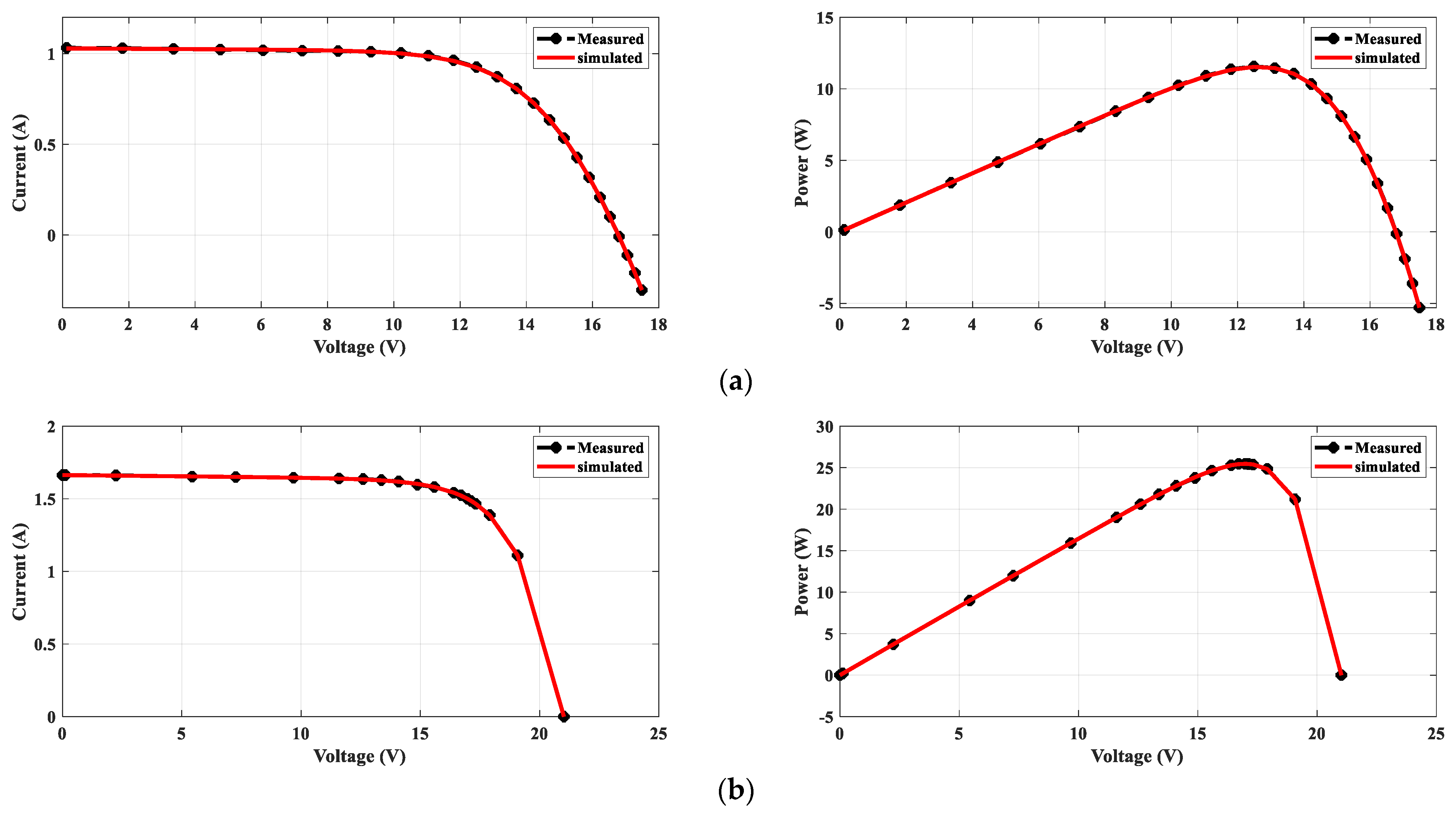
6.1. Case 1: Constant Weather Conditions
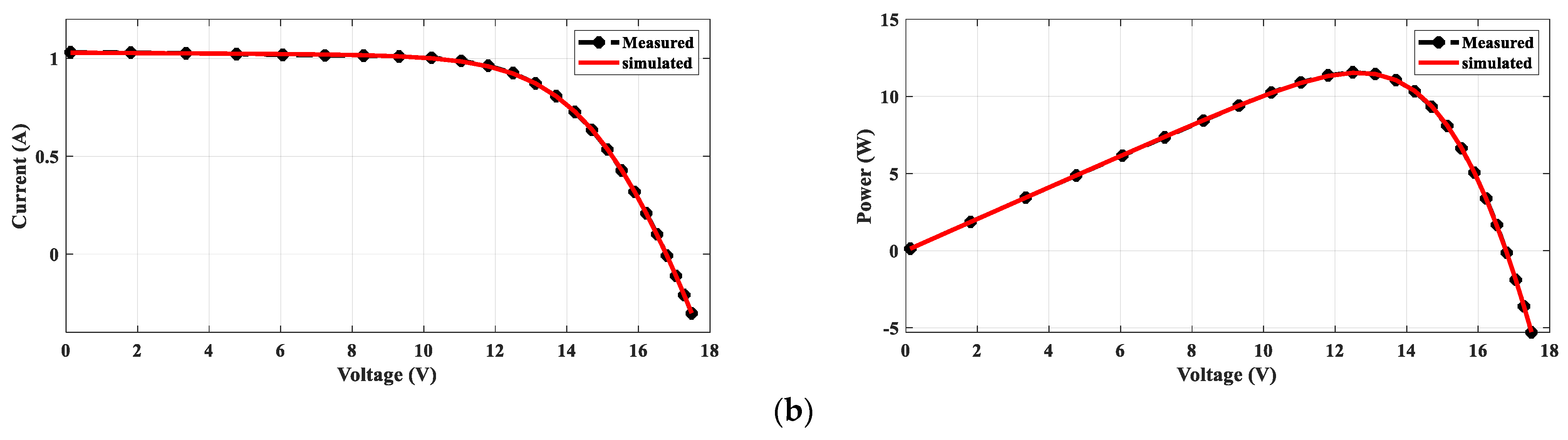
6.1.1. PVW 752 Cell
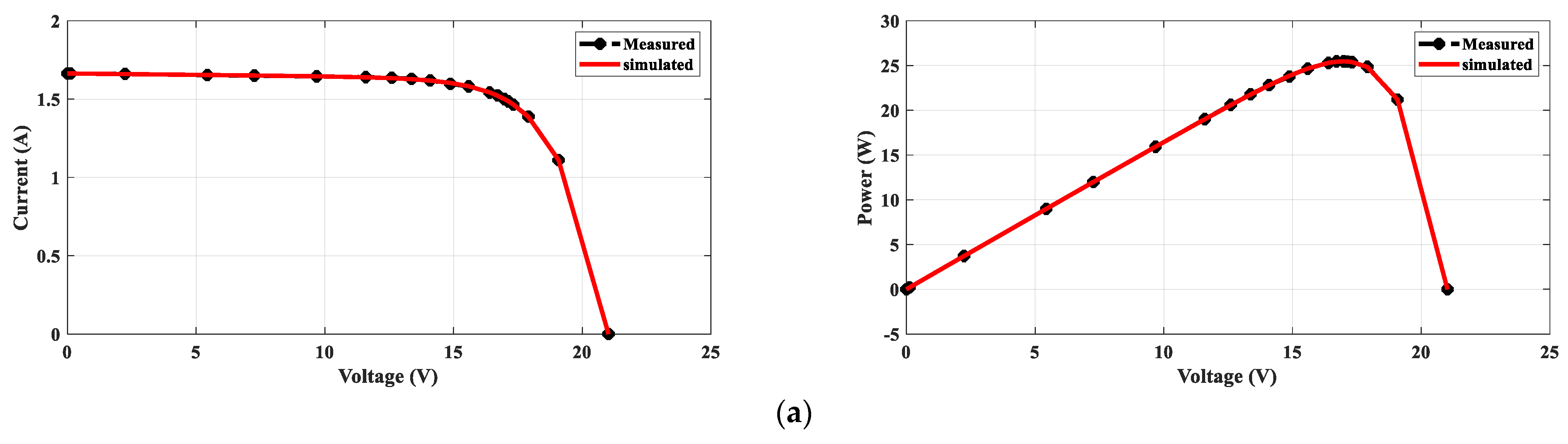
6.1.2. PV Panel
6.2. Case 2: Variable Weather Conditions
7. Conclusions
- For the PVW 752 cell, the proposed HGTO-BWO achieved the best fitness values of 1.527 × 10⁻⁴ and 2.0886 × 10⁻⁴ for the TDM and DDM, respectively.
- The proposed approach achieved the lowest RMSEs of 2.42508 × 10⁻³ for the PWP-201 and 1.8032 × 10⁻³ for the STM6-40/36 DDM.
- The HGTO-BWO achieved the best fitness values of 2.2068 × 10⁻³ for the PWP-201 panel and 1.7435 × 10⁻³ for the STM6-40/36 TDM.
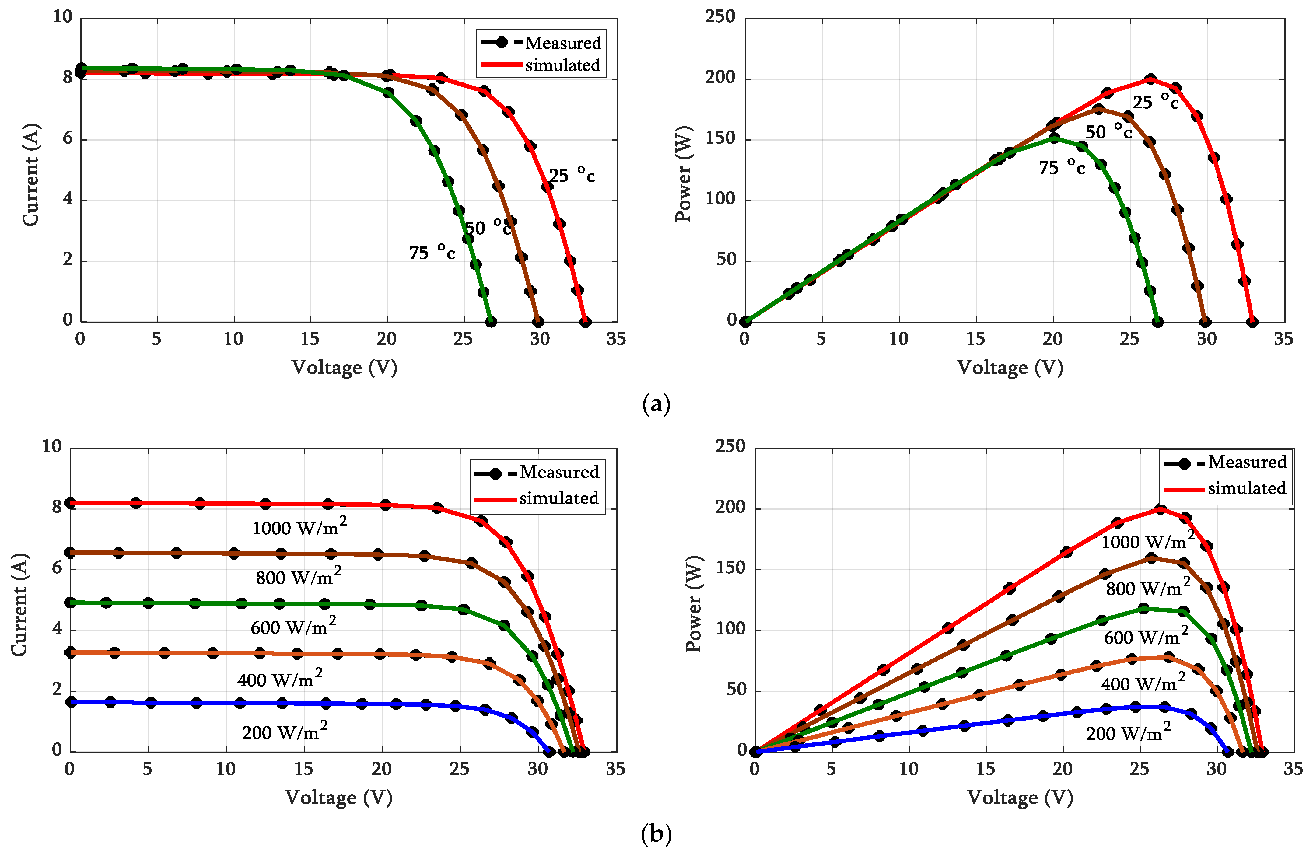
- For KC200GT, the minimum fitness values were 2.3850 × 10⁻⁴, 7.7891 × 10⁻⁴, 6.3910 × 10⁻⁴, and 9.1596 × 10⁻⁴ during operation at 200 W/m2, 400 W/m2, 600 W/m2, and 800 W/m2, respectively.
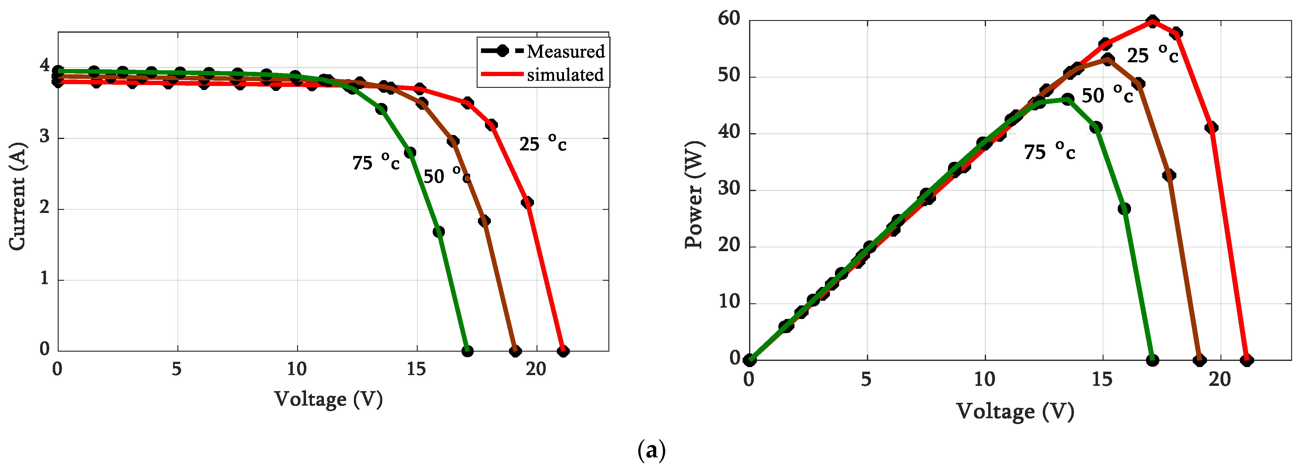
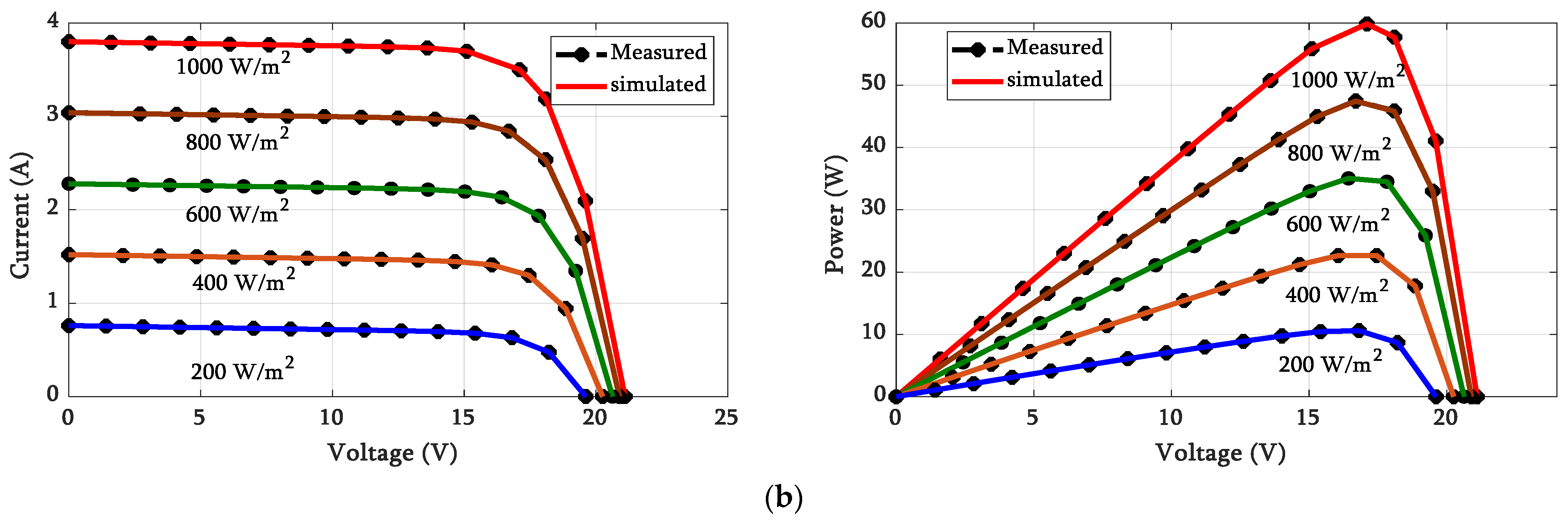
- For MSX60, the proposed methodology realized the best RMSE values of 1.0765 × 10⁻⁴, 1.9324 × 10⁻⁴, and 2.9790 × 10⁻⁵ at 25 °C, 50 °C, and 75 °C, respectively, while at 25 °C the fitness values were 1.1336 × 10⁻³ at 800 W/m2, 6.7775 × 10⁻⁴ at 600 W/m2, 2.4366 × 10⁻⁵ at 400 W/m2, and 5.9828 × 10⁻⁵ at 200 W/m2.
Supplementary Materials
Author Contributions
Funding
Institutional Review Board Statement
Informed Consent Statement
Data Availability Statement
Conflicts of Interest
Appendix A

| Algorithms | Parameter | All Algorithms |
|---|---|---|
| TSA | pmin = 1, pmax = 4 | Pop.size = 30 Max_Iter = 500 No. Run = 30 |
| SCA | a = 2 | |
| GWO | a = 2 to 0 | |
| WOA | a = 2 to 0, a2 = −1 to −2, b = 1 | |
| HS | HMCR = 0.8, PAR = 0.2, FW_d = 0.995 | |
| BWO | Wf = [0.1 0.05] | |
| GTO | β = 3, p = 0.03, w = 0.8 |
References
- Long, W.; Jiao, J.; Liang, X.; Xu, M.; Tang, M.; Cai, S. Parameters Estimation of Photovoltaic Models Using a Novel Hybrid Seagull Optimization Algorithm. Energy 2022, 249, 123760. [Google Scholar] [CrossRef]
- D’Adamo, I.; Mammetti, M.; Ottaviani, D.; Ozturk, I. Photovoltaic Systems and Sustainable Communities: New Social Models for Ecological Transition. The Impact of Incentive Policies in Profitability Analyses. Renew. Energy 2023, 202, 1291–1304. [Google Scholar] [CrossRef]
- D’Adamo, I.; Gastaldi, M.; Morone, P.; Ozturk, I. Economics and Policy Implications of Residential Photovoltaic Systems in Italy’s Developed Market. Util. Policy 2022, 79, 101437. [Google Scholar] [CrossRef]
- Ganesan, S.; David, P.W.; Balachandran, P.K.; Senjyu, T. Fault Identification Scheme for Solar Photovoltaic Array in Bridge and Honeycomb Configuration. Electr. Eng. 2023. [Google Scholar] [CrossRef]
- Ayyarao, T.S.L.V.; Kumar, P.P. Parameter Estimation of Solar PV Models with a New Proposed War Strategy Optimization Algorithm. Int. J. Energy Res. 2022, 46, 7215–7238. [Google Scholar] [CrossRef]
- Shaheen, M.A.M.; Hasanien, H.M.; Alkuhayli, A. A Novel Hybrid GWO-PSO Optimization Technique for Optimal Reactive Power Dispatch Problem Solution. Ain Shams Eng. J. 2021, 12, 621–630. [Google Scholar] [CrossRef]
- Vankadara, S.K.; Chatterjee, S.; Balachandran, P.K.; Mihet-Popa, L. Marine Predator Algorithm (MPA)-Based MPPT Technique for Solar PV Systems under Partial Shading Conditions. Energies 2022, 15, 6172. [Google Scholar] [CrossRef]
- Libra, M.; Mrázek, D.; Tyukhov, I.; Severová, L.; Poulek, V.; Mach, J.; Šubrt, T.; Beránek, V.; Svoboda, R.; Sedláček, J. Reduced Real Lifetime of PV Panels—Economic Consequences. Sol. Energy 2023, 259, 229–234. [Google Scholar] [CrossRef]
- Pourmousa, N.; Ebrahimi, S.M.; Malekzadeh, M.; Gordillo, F. Using a Novel Optimization Algorithm for Parameter Extraction of Photovoltaic Cells and Modules. Eur. Phys. J. Plus 2021, 136, 470. [Google Scholar] [CrossRef]
- Nayagam, V.S.; Kumar, S.S.; Thiyagarajan, V.; Kamal, N.; Nisha, N.; Isaac, J.S.; Kassa, A. A Novel Optimization Algorithm for Modifying the Parameter Unit of Solar PV Cell. Int. J. Photoenergy 2022, 2022, 5240115. [Google Scholar] [CrossRef]
- Prince Winston, D.; Kumaravel, S.; Praveen Kumar, B.; Devakirubakaran, S. Performance Improvement of Solar PV Array Topologies during Various Partial Shading Conditions. Sol. Energy 2020, 196, 228–242. [Google Scholar] [CrossRef]
- Vankadara, S.K.; Chatterjee, S.; Balachandran, P.K. An Accurate Analytical Modeling of Solar Photovoltaic System Considering Rs and Rsh under Partial Shaded Condition. Int. J. Syst. Assur. Eng. Manag. 2022, 13, 2472–2481. [Google Scholar] [CrossRef]
- Gude, S.; Jana, K.C. Parameter Extraction of Photovoltaic Cell Using an Improved Cuckoo Search Optimization. Sol. Energy 2020, 204, 280–293. [Google Scholar] [CrossRef]
- Wang, L.; Chen, Z.; Guo, Y.; Hu, W.; Chang, X.; Wu, P.; Han, C.; Li, J. Accurate Solar Cell Modeling via Genetic Neural Network-Based Meta-Heuristic Algorithms. Front. Energy Res. 2021, 9, 1–14. [Google Scholar] [CrossRef]
- Repalle, N.B.; Sarala, P.; Mihet-Popa, L.; Kotha, S.R.; Rajeswaran, N. Implementation of a Novel Tabu Search Optimization Algorithm to Extract Parasitic Parameters of Solar Panel. Energies 2022, 15, 4515. [Google Scholar] [CrossRef]
- Sarjila, R.; Ravi, K.; Edward, J.B.; Kumar, K.S.; Prasad, A. Parameter Extraction of Solar Photovoltaic Modules Using Gravitational Search Algorithm. J. Electr. Comput. Eng. 2016, 2016, 2143572. [Google Scholar] [CrossRef] [Green Version]
- Singh, A.; Sharma, A.; Rajput, S.; Mondal, A.K.; Bose, A.; Ram, M. Parameter Extraction of Solar Module Using the Sooty Tern Optimization Algorithm. Electronics 2022, 11, 564. [Google Scholar] [CrossRef]
- Singla, M.K.; Nijhawan, P.; Oberoi, A.S. A Novel Hybrid Particle Swarm Optimization Rat Search Algorithm for Parameter Estimation of Solar PV and Fuel Cell Model. COMPEL—Int. J. Comput. Math. Electr. Electron. Eng. 2022, 41, 1505–1527. [Google Scholar] [CrossRef]
- Ridhor, S.I.A.; Isa, Z.M.; Nayan, N.M. Parameter Extraction of PV Cell Single Diode Model Using Animal Migration Optimization. Int. J. Electr. Eng. Appl. Sci. 2020, 3, 1–6. [Google Scholar]
- Oliva, D.; Abd El Aziz, M.; Ella Hassanien, A. Parameter Estimation of Photovoltaic Cells Using an Improved Chaotic Whale Optimization Algorithm. Appl. Energy 2017, 200, 141–154. [Google Scholar] [CrossRef]
- Ramadan, T.; Kamel, S.; Neggaz, N.; Alghamdi, A.S. Developing Photovoltaic Cells Parameter Estimation Algorithm Based on Equilibrium Optimization Technique. J. Eng. Res. 2021, 10, 1–27. [Google Scholar] [CrossRef]
- Saha, C.; Agbu, N.; Jinks, R. 2—Review Article of the Solar PV Parameters Estimation Using Evolutionary Algorithms. MOJ Sol. Photoen Sys. 2018, 2, 66–78. [Google Scholar] [CrossRef]
- Ahmed, W.A.E.M.; Mageed, H.M.A.; Mohamed, S.A.E.; Saleh, A.A. Fractional Order Darwinian Particle Swarm Optimization for Parameters Identification of Solar PV Cells and Modules. Alexandria Eng. J. 2022, 61, 1249–1263. [Google Scholar] [CrossRef]
- Rawa, M.; Abusorrah, A.; Al-Turki, Y.; Calasan, M.; Micev, M.; Ali, Z.M.; Mekhilef, S.; Bassi, H.; Sindi, H.; Abdel Aleem, S.H.E. Estimation of Parameters of Different Equivalent Circuit Models of Solar Cells and Various Photovoltaic Modules Using Hybrid Variants of Honey Badger Algorithm and Artificial Gorilla Troops Optimizer. Mathematics 2022, 10, 1057. [Google Scholar] [CrossRef]
- Ginidi, A.; Ghoneim, S.M.; Elsayed, A.; El-Sehiemy, R.; Shaheen, A.; El-Fergany, A. Gorilla Troops Optimizer for Electrically Based Single and Double-Diode Models of Solar Photovoltaic Systems. Sustainability 2021, 13, 9459. [Google Scholar] [CrossRef]
- Bayoumi, A.S.A.; El-Sehiemy, R.A.; Abaza, A. Effective PV Parameter Estimation Algorithm Based on Marine Predators Optimizer Considering Normal and Low Radiation Operating Conditions. Arab. J. Sci. Eng. 2022, 47, 3089–3104. [Google Scholar] [CrossRef]
- El Sattar, M.A.; Al Sumaiti, A.; Ali, H.; Diab, A.A.Z. Marine Predators Algorithm for Parameters Estimation of Photovoltaic Modules Considering Various Weather Conditions. Neural Comput. Appl. 2021, 33, 11799–11819. [Google Scholar] [CrossRef]
- Rezk, H.; Abdelkareem, M.A. Optimal Parameter Identification of Triple Diode Model for Solar Photovoltaic Panel and Cells. Energy Rep. 2022, 8, 1179–1188. [Google Scholar] [CrossRef]
- Xu, S.; Qiu, H. A Modified Stochastic Fractal Search Algorithm for Parameter Estimation of Solar Cells and PV Modules. Energy Rep. 2022, 8, 1853–1866. [Google Scholar] [CrossRef]
- Abbassi, A.; Ben Mehrez, R.; Touaiti, B.; Abualigah, L.; Touti, E. Parameterization of Photovoltaic Solar Cell Double-Diode Model Based on Improved Arithmetic Optimization Algorithm. Optik (Stuttg). 2022, 253, 168600. [Google Scholar] [CrossRef]
- Muhammadsharif, F.F. A New Simplified Method for Efficient Extraction of Solar Cells and Modules Parameters from Datasheet Information. Silicon 2022, 14, 3059–3067. [Google Scholar] [CrossRef]
- Lin, X.; Wu, Y. Parameters Identification of Photovoltaic Models Using Niche-Based Particle Swarm Optimization in Parallel Computing Architecture. Energy 2020, 196, 117054. [Google Scholar] [CrossRef]
- Gude, S.; Jana, K.C. A Multiagent System Based Cuckoo Search Optimization for Parameter Identification of Photovoltaic Cell Using Lambert W-Function. Appl. Soft Comput. 2022, 120, 108678. [Google Scholar] [CrossRef]
- Ali, F.; Sarwar, A.; Ilahi Bakhsh, F.; Ahmad, S.; Ali Shah, A.; Ahmed, H. Parameter Extraction of Photovoltaic Models Using Atomic Orbital Search Algorithm on a Decent Basis for Novel Accurate RMSE Calculation. Energy Convers. Manag. 2023, 277, 116613. [Google Scholar] [CrossRef]
- Beşkirli, A.; Dağ, İ. Parameter Extraction for Photovoltaic Models with Tree Seed Algorithm. Energy Rep. 2023, 9, 174–185. [Google Scholar] [CrossRef]
- Wang, D.; Sun, X.; Kang, H.; Shen, Y.; Chen, Q. Heterogeneous Differential Evolution Algorithm for Parameter Estimation of Solar Photovoltaic Models. Energy Rep. 2022, 8, 4724–4746. [Google Scholar] [CrossRef]
- Yu, Y.; Wang, K.; Zhang, T.; Wang, Y.; Peng, C.; Gao, S. A Population Diversity-Controlled Differential Evolution for Parameter Estimation of Solar Photovoltaic Models. Sustain. Energy Technol. Assess. 2022, 51, 101938. [Google Scholar] [CrossRef]
- Alanazi, M.; Alanazi, A.; Almadhor, A.; Rauf, H.T. Photovoltaic Models’ Parameter Extraction Using New Artificial Parameterless Optimization Algorithm. Mathematics 2022, 10, 4617. [Google Scholar] [CrossRef]
- Fan, Y.; Wang, P.; Heidari, A.A.; Chen, H.; HamzaTurabieh; Mafarja, M. Random Reselection Particle Swarm Optimization for Optimal Design of Solar Photovoltaic Modules. Energy 2022, 239, 121865. [Google Scholar] [CrossRef]
- Ridha, H.M.; Hizam, H.; Mirjalili, S.; Othman, M.L.; Ya’acob, M.E.; Abualigah, L. A Novel Theoretical and Practical Methodology for Extracting the Parameters of the Single and Double Diode Photovoltaic Models (December 2021). IEEE Access 2022, 10, 11110–11137. [Google Scholar] [CrossRef]
- Lin, H.; Ahmadianfar, I.; Amiri Golilarz, N.; Jamei, M.; Heidari, A.A.; Kuang, F.; Zhang, S.; Chen, H. Adaptive Slime Mould Algorithm for Optimal Design of Photovoltaic Models. Energy Sci. Eng. 2022, 10, 2035–2064. [Google Scholar] [CrossRef]
- Chen, N.; Bi, W.; Xu, G.; Wu, Z.; Wu, M.; Luo, K. Mayfly Optimization Algorithm–Based PV Cell Triple-Diode Model Parameter Identification. Front. Energy Res. 2022, 10, 1–10. [Google Scholar] [CrossRef]
- El-Dabah, M.A.; El-Sehiemy, R.A.; Hasanien, H.M.; Saad, B. Photovoltaic Model Parameters Identification Using Northern Goshawk Optimization Algorithm. Energy 2023, 262, 125522. [Google Scholar] [CrossRef]
- Kumar, C.; Magdalin Mary, D. A Novel Chaotic-Driven Tuna Swarm Optimizer with Newton-Raphson Method for Parameter Identification of Three-Diode Equivalent Circuit Model of Solar Photovoltaic Cells/Modules. Optik (Stuttg). 2022, 264, 169379. [Google Scholar] [CrossRef]
- Bo, Q.; Cheng, W.; Khishe, M.; Mohammadi, M.; Mohammed, A.H. Solar Photovoltaic Model Parameter Identification Using Robust Niching Chimp Optimization. Sol. Energy 2022, 239, 179–197. [Google Scholar] [CrossRef]
- Gupta, J.; Hussain, A.; Singla, M.K.; Nijhawan, P.; Haider, W.; Kotb, H.; AboRas, K.M. Parameter Estimation of Different Photovoltaic Models Using Hybrid Particle Swarm Optimization and Gravitational Search Algorithm. Appl. Sci. 2023, 13, 249. [Google Scholar] [CrossRef]
- Ramadan, A.; Kamel, S.; Hussein, M.M.; Hassan, M.H. A New Application of Chaos Game Optimization Algorithm for Parameters Extraction of Three Diode Photovoltaic Model. IEEE Access 2021, 9, 51582–51594. [Google Scholar] [CrossRef]
- Yu, S.; Chen, Z.; Heidari, A.A.; Zhou, W.; Chen, H.; Xiao, L. Parameter Identification of Photovoltaic Models Using a Sine Cosine Differential Gradient Based Optimizer. IET Renew. Power Gener. 2022, 16, 1535–1561. [Google Scholar] [CrossRef]
- Jiang, Y.; Luo, Q.; Zhou, Y. Improved Gradient-based Optimizer for Parameters Extraction of Photovoltaic Models. IET Renew. Power Gener. 2022, 16, 1602–1622. [Google Scholar] [CrossRef]
- Wang, J.; Yang, B.; Li, D.; Zeng, C.; Chen, Y.; Guo, Z.; Zhang, X.; Tan, T.; Shu, H.; Yu, T. Photovoltaic Cell Parameter Estimation Based on Improved Equilibrium Optimizer Algorithm. Energy Convers. Manag. 2021, 236, 114051. [Google Scholar] [CrossRef]
- Shaheen, A.M.; Ginidi, A.R.; El-Sehiemy, R.A.; Ghoneim, S.S.M. A Forensic-Based Investigation Algorithm for Parameter Extraction of Solar Cell Models. IEEE Access 2021, 9, 1–20. [Google Scholar] [CrossRef]
- Shaheen, A.M.; El-Seheimy, R.A.; Xiong, G.; Elattar, E.; Ginidi, A.R. Parameter Identification of Solar Photovoltaic Cell and Module Models via Supply Demand Optimizer. Ain Shams Eng. J. 2022, 13, 101705. [Google Scholar] [CrossRef]
- Yu, S.; Heidari, A.A.; He, C.; Cai, Z.; Althobaiti, M.M.; Mansour, R.F.; Liang, G.; Chen, H. Parameter Estimation of Static Solar Photovoltaic Models Using Laplacian Nelder-Mead Hunger Games Search. Sol. Energy 2022, 242, 79–104. [Google Scholar] [CrossRef]
- Lekouaghet, B.; Boukabou, A.; Boubakir, C. Estimation of the Photovoltaic Cells/Modules Parameters Using an Improved Rao-Based Chaotic Optimization Technique. Energy Convers. Manag. 2021, 229, 113722. [Google Scholar] [CrossRef]
- Ridha, H.M.; Hizam, H.; Mirjalili, S.; Othman, M.L.; Ya’acob, M.E.; Ahmadipour, M. Parameter Extraction of Single, Double, and Three Diodes Photovoltaic Model Based on Guaranteed Convergence Arithmetic Optimization Algorithm and Modified Third Order Newton Raphson Methods. Renew. Sustain. Energy Rev. 2022, 162, 112436. [Google Scholar] [CrossRef]
- Ibrahim, I.A.; Hossain, M.J.; Duck, B.C. A Hybrid Wind Driven-Based Fruit Fly Optimization Algorithm for Identifying the Parameters of a Double-Diode Photovoltaic Cell Model Considering Degradation Effects. Sustain. Energy Technol. Assessments 2022, 50, 101685. [Google Scholar] [CrossRef]
- Saha, A.K. Multi-Population-Based Adaptive Sine Cosine Algorithm with Modified Mutualism Strategy for Global Optimization. Knowl. -Based Syst. 2022, 251, 109326. [Google Scholar] [CrossRef]
- Ma, H.; Shen, S.; Yu, M.; Yang, Z.; Fei, M.; Zhou, H. Multi-Population Techniques in Nature Inspired Optimization Algorithms: A Comprehensive Survey. Swarm Evol. Comput. 2019, 44, 365–387. [Google Scholar] [CrossRef]
- Satria, H.; Syah, R.B.Y.; Nehdi, M.L.; Almustafa, M.K.; Adam, A.O.I. Parameters Identification of Solar PV Using Hybrid Chaotic Northern Goshawk and Pattern Search. Sustainability 2023, 15, 5027. [Google Scholar] [CrossRef]
- Ben Aribia, H.; El-Rifaie, A.M.; Tolba, M.A.; Shaheen, A.; Moustafa, G.; Elsayed, F.; Elshahed, M. Growth Optimizer for Parameter Identification of Solar Photovoltaic Cells and Modules. Sustainability 2023, 15, 7896. [Google Scholar] [CrossRef]
- Bogar, E. Chaos Game Optimization-Least Squares Algorithm for Photovoltaic Parameter Estimation. Arab. J. Sci. Eng. 2023, 48, 6321–6340. [Google Scholar] [CrossRef]
- Rawat, N.; Thakur, P.; Singh, A.K.; Bhatt, A.; Sangwan, V.; Manivannan, A. A New Grey Wolf Optimization-Based Parameter Estimation Technique of Solar Photovoltaic. Sustain. Energy Technol. Assess. 2023, 57, 103240. [Google Scholar] [CrossRef]
- Qaraad, M.; Amjad, S.; Hussein, N.K.; Badawy, M.; Mirjalili, S.; Elhosseini, M.A. Photovoltaic Parameter Estimation Using Improved Moth Flame Algorithms with Local Escape Operators. Comput. Electr. Eng. 2023, 106, 108603. [Google Scholar] [CrossRef]
- Changmai, P.; Deka, S.; Kumar, S.; Babu, T.S.; Aljafari, B.; Nastasi, B. A Critical Review on the Estimation Techniques of the Solar PV Cell’s Unknown Parameters. Energies 2022, 15, 7212. [Google Scholar] [CrossRef]
- Yang, B.; Wang, J.; Zhang, X.; Yu, T.; Yao, W.; Shu, H.; Zeng, F.; Sun, L. Comprehensive Overview of Meta-Heuristic Algorithm Applications on PV Cell Parameter Identification. Energy Convers. Manag. 2020, 208, 112595. [Google Scholar] [CrossRef]
- Ali, H.H.; Fathy, A.; Al-dhaifallah, M.; Abdelaziz, A.Y.; Ebeed, M. An Efficient Capuchin Search Algorithm for Extracting the Parameters of Different PV Cells / Modules. Front. Energy Res. 2022, 10, 1028816. [Google Scholar] [CrossRef]
- Diab, A.A.Z.; Ezzat, A.; Rafaat, A.E.; Denis, K.A.; Abdelsalam, H.A.; Abdelhamid, A.M. Optimal Identification of Model Parameters for PVs Using Equilibrium, Coot Bird and Artificial Ecosystem Optimisation Algorithms. IET Renew. Power Gener. 2022, 16, 2172–2190. [Google Scholar] [CrossRef]
- Fathy, A.; Rezk, H. Parameter Estimation of Photovoltaic System Using Imperialist Competitive Algorithm. Renew. Energy 2017, 111, 307–320. [Google Scholar] [CrossRef]
- Abdollahzadeh, B.; Gharehchopogh, F.S.; Mirjalili, S. Artificial Gorilla Troops Optimizer: A New Nature-inspired Metaheuristic Algorithm for Global Optimization Problems. Int. J. Intell. Syst. 2021, 36, 5887–5958. [Google Scholar] [CrossRef]
- Zhong, C.; Li, G.; Meng, Z. Beluga Whale Optimization: A Novel Nature-Inspired Metaheuristic Algorithm. Knowledge-Based Syst. 2022, 251, 109215. [Google Scholar] [CrossRef]
- Mirjalili, S.; Mirjalili, S.M.; Lewis, A. Grey Wolf Optimizer. Adv. Eng. Softw. 2014, 69, 46–61. [Google Scholar] [CrossRef] [Green Version]
- Szabo, R.; Gontean, A. Photovoltaic Cell and Module I-V Characteristic Approximation Using Bézier Curves. Appl. Sci. 2018, 8, 655. [Google Scholar] [CrossRef] [Green Version]
- Abdullah, J.M.; Ahmed, T. Fitness Dependent Optimizer: Inspired by the Bee Swarming Reproductive Process. IEEE Access 2019, 7, 43473–43486. [Google Scholar] [CrossRef]
- Premkumar, M.; Jangir, P.; Ramakrishnan, C.; Nalinipriya, G.; Alhelou, H.H.; Kumar, B.S. Identification of Solar Photovoltaic Model Parameters Using an Improved Gradient-Based Optimization Algorithm with Chaotic Drifts. IEEE Access 2021, 9, 62347–62379. [Google Scholar] [CrossRef]
- Darmansyah; Robandi, I. Photovoltaic Parameter Estimation Using Grey Wolf Optimization. In Proceedings of the 2017 3rd International Conference on Control, Automation and Robotics (ICCAR), Nagoya, Japan, 24-26 April 2017; pp. 593–597. [Google Scholar] [CrossRef]
- Elazab, O.S.; Hasanien, H.M.; Elgendy, M.A.; Abdeen, A.M. Whale Optimisation Algorithm for Photovoltaic Model Identification. J. Eng. 2017, 2017, 1906–1911. [Google Scholar] [CrossRef]
- Naeijian, M.; Rahimnejad, A.; Ebrahimi, S.M.; Pourmousa, N.; Gadsden, S.A. Parameter Estimation of PV Solar Cells and Modules Using Whippy Harris Hawks Optimization Algorithm. Energy Rep. 2021, 7, 4047–4063. [Google Scholar] [CrossRef]
- Libra, M.; Petrik, T.; Poulek, V.; Tyukhov, I.I.; Kourim, P. Changes in the Efficiency of Photovoltaic Energy Conversion in Temperature Range with Extreme Limits. IEEE J. Photovolt. 2021, 11, 1479–1484. [Google Scholar] [CrossRef]
- Arias García, R.M.; Pérez Abril, I. Photovoltaic Module Model Determination by Using the Tellegen’s Theorem. Renew. Energy 2020, 152, 409–420. [Google Scholar] [CrossRef]


| Ref. | Obj. Function | Model Type | Algorithm | Remark |
|---|---|---|---|---|
| [59] | RMSE | SDM, DDM and TDM | Hybrid chaotic NSO-PS | One type of PV is R.T.C used in all case studies; complexity and improved performance |
| [60] | RMSE | SDM and DDM | Growth optimizer | Ability to determine ungiven PV model parameters; low convergence |
| [61] | RMSE | SDM, DDM, and TDM | Chaos game optimization with least squares | Speed convergence and the RMSE values are similar to those of some other methods |
| [62] | Non-linear square with RMSE | SDM | GWO | Complexity in obj. function |
| [63] | RMSE | SDM, DDM, and TDM | Improved moth–flame algorithms | Low obj. function |
| Proposed | RMSE | SDM, DDM and TDM | HGTO-BWO | High performance and efficiency; avoids local optimum; fast convergence |
| Function No | Algorithm | Worst | Mean | Best | std | p-Value |
|---|---|---|---|---|---|---|
| F1 | TSA | 6.062× 10⁻²¹ | 8.593 × 10⁻²² | 1.829 × 10⁻²⁴ | 1.367 × 10⁻²¹ | 1.21 × 10⁻¹² |
| GWO | 3.300 × 10⁻²⁶ | 2.105 × 10⁻²⁷ | 4.759 × 10⁻²⁹ | 6.022 × 10⁻²⁷ | 1.21 × 10⁻¹² | |
| WOA | 6.553 × 10−70 | 2.364 × 10−71 | 2.778 × 10−83 | 1.197 × 10−70 | 1.21 × 10⁻¹² | |
| SCA | 4.516 × 10² | 3.588 × 101 | 2.339 × 10⁻² | 1.003 × 10² | 1.21 × 10⁻¹² | |
| HS | 3.079 × 10³ | 2.476 × 10³ | 1.562 × 10³ | 3.939 × 10² | 1.21 × 10⁻¹² | |
| BWO | 1.925 × 10−257 | 1.272 × 10−258 | 1.274 × 10−272 | 0.00 × 100 | 1.21 × 10⁻¹² | |
| GTO | 0.00 × 100 | 0.00 × 100 | 0.00 × 100 | 0.00 × 100 | 1.21 × 10⁻¹² | |
| HGTO-BWO | 0.00 × 100 | 0.00 × 100 | 0.00 × 100 | 0.00 × 100 | NAN | |
| F2 | TSA | 4.979 × 10⁻¹³ | 1.128 × 10⁻¹³ | 1.047 × 10⁻¹⁴ | 1.206 × 10⁻¹³ | 3.02 × 10⁻¹¹ |
| GWO | 4.515 × 10⁻¹⁶ | 9.566 × 10⁻¹⁷ | 1.246 × 10⁻¹⁷ | 8.300 × 10⁻¹⁷ | 3.02 × 10⁻¹¹ | |
| WOA | 1.156 × 10−48 | 7.100 × 10−50 | 1.076 × 10−56 | 2.454 × 10−49 | 3.02 × 10⁻¹¹ | |
| SCA | 1.346 × 10⁻¹ | 2.449 × 10⁻² | 8.107 × 10⁻⁵ | 3.647 × 10⁻² | 3.02 × 10⁻¹¹ | |
| HS | 1.370 × 101 | 1.057 × 101 | 7.436 × 100 | 1.673 × 100 | 3.02 × 10⁻¹¹ | |
| BWO | 1.849 × 10−129 | 6.467 × 10−131 | 1.310 × 10−137 | 3.37 × 10−130 | 3.02 × 10⁻¹¹ | |
| GTO | 1.835 × 10−190 | 6.261 × 10−192 | 3.521 × 10−206 | 0.00 × 100 | 3.02 × 10⁻¹¹ | |
| HGTO-BWO | 6.916 × 10−247 | 2.305 × 10−248 | 5.079 × 10−268 | 0.00 × 100 | NAN | |
| F3 | TSA | 2.826 × 10⁻³ | 3.329 × 10⁻⁴ | 1.572 × 10⁻⁸ | 7.279 × 10⁻⁴ | 1.21 × 10⁻¹² |
| GWO | 3.698 × 10⁻⁴ | 2.062 × 10⁻⁵ | 7.248 × 10⁻⁹ | 6.741 × 10⁻⁵ | 1.21 × 10⁻¹² | |
| WOA | 7.244 × 10⁴ | 3.723 × 10⁴ | 2.987 × 10³ | 1.716 × 10⁴ | 1.21 × 10⁻¹² | |
| SCA | 2.274 × 10⁴ | 9.511 × 10³ | 1.459 × 10³ | 5.359 × 10³ | 1.21 × 10⁻¹² | |
| HS | 3.362 × 10⁴ | 2.686 × 10⁴ | 1.965 × 10⁴ | 3.983 × 10³ | 1.21 × 10⁻¹² | |
| BWO | 1.555 × 10−242 | 1.060 × 10−243 | 2.864 × 10−257 | 0.00 × 100 | 1.21 × 10⁻¹² | |
| GTO | 0.00 × 100 | 0.00 × 100 | 0.00 × 100 | 0.00 × 100 | 1.21 × 10⁻¹² | |
| HGTO-BWO | 0.00 × 100 | 0.00 × 100 | 0.00 × 100 | 0.00 × 100 | NAN | |
| F4 | TSA | 7.663 × 10⁻¹ | 2.588 × 10⁻¹ | 1.258 × 10⁻² | 2.234 × 10⁻¹ | 3.02 × 10⁻¹¹ |
| GWO | 7.987 × 10⁻⁶ | 8.996 × 10⁻⁷ | 4.183 × 10⁻⁸ | 1.485 × 10⁻⁶ | 3.02 × 10⁻¹¹ | |
| WOA | 9.425 × 101 | 5.178 × 101 | 7.053 × 10⁻² | 3.113 × 101 | 3.02 × 10⁻¹¹ | |
| SCA | 5.758 × 101 | 3.099 × 101 | 1.005 × 101 | 1.173 × 101 | 3.02 × 10⁻¹¹ | |
| HS | 4.145 × 101 | 3.622 × 101 | 3.042 × 101 | 2.199 × 100 | 3.02 × 10⁻¹¹ | |
| BWO | 3.880 × 10−126 | 3.095 × 10−127 | 2.571 × 10−133 | 7.804 × 10−127 | 3.02 × 10⁻¹¹ | |
| GTO | 1.694 × 10−192 | 8.353 × 10−194 | 9.838 × 10−208 | 0.00 × 100 | 3.02 × 10⁻¹¹ | |
| HGTO-BWO | 6.349 × 10−238 | 2.187 × 10−239 | 5.440 × 10−257 | 0.00 × 100 | NAN | |
| F5 | TSA | 2.889 × 101 | 2.838 × 101 | 2.609 × 101 | 7.737 × 10⁻¹ | 2.37 × 10⁻¹² |
| GWO | 2.852 × 101 | 2.682 × 101 | 2.566 × 101 | 7.761 × 10⁻¹ | 2.37 × 10⁻¹² | |
| WOA | 2.877 × 101 | 2.794 × 101 | 2.728 × 101 | 5.032 × 10⁻¹ | 2.37 × 10⁻¹² | |
| SCA | 4.983 × 10⁵ | 4.696 × 10⁴ | 1.048 × 10² | 9.858 × 10⁴ | 2.37 × 10⁻¹² | |
| HS | 1.768 × 10⁶ | 1.070 × 10⁶ | 6.292 × 10⁵ | 2.773 × 10⁵ | 2.37 × 10⁻¹² | |
| BWO | 8.153 × 10⁻⁶ | 1.346 × 10⁻⁶ | 1.618 × 10⁻⁹ | 2.176 × 10⁻⁶ | 2.37 × 10⁻¹² | |
| GTO | 2.477 × 101 | 2.445 × 100 | 6.987 × 10⁻⁸ | 7.461 × 100 | 2.37 × 10⁻¹² | |
| HGTO-BWO | 1.395 × 10⁻²⁸ | 5.853 × 10⁻³⁰ | 0.00 × 100 | 2.608 × 10⁻²⁹ | NAN | |
| F6 | TSA | 4.820 × 100 | 3.817 × 100 | 2.590 × 100 | 6.004 × 10⁻¹ | 1.212 × 10⁻¹² |
| GWO | 1.754 × 100 | 8.393 × 10⁻¹ | 6.737 × 10⁻⁵ | 4.021 × 10⁻¹ | 1.212 × 10⁻¹² | |
| WOA | 9.864 × 10⁻¹ | 3.725 × 10⁻¹ | 1.355 × 10⁻¹ | 1.979 × 10⁻¹ | 1.212 × 10⁻¹² | |
| SCA | 2.624 × 10² | 2.762 × 101 | 4.337 × 100 | 4.997 × 101 | 1.212 × 10⁻¹² | |
| HS | 3.225 × 10³ | 2.582 × 10³ | 1.422 × 10³ | 4.447 × 10² | 1.212 × 10⁻¹² | |
| BWO | 2.490 × 10⁻¹³ | 1.879 × 10⁻¹⁴ | 1.153 × 10⁻¹⁷ | 4.703 × 10⁻¹⁴ | 1.212 × 10⁻¹² | |
| GTO | 7.369 × 10⁻⁷ | 1.292 × 10⁻⁷ | 7.310 × 10⁻¹¹ | 1.675 × 10⁻⁷ | 1.212 × 10⁻¹² | |
| HGTO-BWO | 0.00 × 100 | 0.00 × 100 | 0.00 × 100 | 0.00 × 100 | NAN | |
| F7 | TSA | 2.022 × 10⁻² | 9.471 × 10⁻³ | 1.816 × 10⁻³ | 4.734 × 10⁻³ | 3.02 × 10⁻¹¹ |
| GWO | 6.588 × 10⁻³ | 1.963 × 10⁻³ | 6.607 × 10⁻⁴ | 1.299 × 10⁻³ | 3.02 × 10⁻¹¹ | |
| WOA | 1.522 × 10⁻² | 3.099 × 10⁻³ | 5.474 × 10⁻⁵ | 3.995 × 10⁻³ | 3.16 × 10⁻¹⁰ | |
| SCA | 4.586 × 10⁻¹ | 8.768 × 10⁻² | 9.960 × 10⁻³ | 9.341 × 10⁻² | 3.02 × 10⁻¹¹ | |
| HS | 1.093 × 100 | 7.266 × 10⁻¹ | 3.535 × 10⁻¹ | 1.790 × 10⁻¹ | 3.02 × 10⁻¹¹ | |
| BWO | 4.232 × 10⁻⁴ | 1.563 × 10⁻⁴ | 3.893 × 10⁻⁷ | 1.160 × 10⁻⁴ | 1.70 × 10⁻² | |
| GTO | 3.524 × 10⁻⁴ | 1.005 × 10⁻⁴ | 1.298 × 10⁻⁵ | 8.193 × 10⁻⁵ | 4.12 × 10⁻¹ | |
| HGTO-BWO | 3.263 × 10⁻⁴ | 8.538 × 10⁻⁵ | 2.321 × 10⁻⁶ | 7.039 × 10⁻⁵ | NAN | |
| F8 | TSA | −4.628 × 10³ | −5.706 × 10³ | −6.921 × 10³ | 5.559 × 10² | 1.720 × 10⁻¹² |
| GWO | −3.023 × 10³ | −6.026 × 10³ | −7.397 × 10³ | 9.273 × 10² | 1.720 × 10⁻¹² | |
| WOA | −6.738 × 10³ | −1.051 × 10⁴ | −1.257 × 10⁴ | 1.872 × 10³ | 1.720 × 10⁻¹² | |
| SCA | −3.240 × 10³ | −3.726 × 10³ | −4.747 × 10³ | 3.438 × 10² | 1.720 × 10⁻¹² | |
| HS | −1.130 × 10⁴ | −1.160 × 10⁴ | −1.196 × 10⁴ | 1.851 × 10² | 1.720 × 10⁻¹² | |
| BWO | −1.257 × 10⁴ | −1.257 × 10⁴ | −1.257 × 10⁴ | 1.548 × 10⁻⁸ | 4.562 × 10⁻¹¹ | |
| GTO | −1.257 × 10⁴ | −1.257 × 10⁴ | −1.257 × 10⁴ | 1.868 × 10⁻⁵ | 4.562 × 10⁻¹¹ | |
| HGTO-BWO | −1.257 × 10⁴ | −1.257 × 10⁴ | −1.257 × 10⁴ | 3.317 × 10⁻³ | NAN | |
| F9 | TSA | 2.745 × 10² | 1.924 × 10² | 1.364 × 10² | 3.806 × 101 | 1.212 × 10⁻¹² |
| GWO | 1.195 × 101 | 2.920 × 100 | 5.684 × 10⁻¹⁴ | 3.451 × 100 | 1.188 × 10⁻¹² | |
| WOA | 5.684 × 10⁻¹⁴ | 1.895 × 10⁻¹⁵ | 0.00 × 100 | 1.038 × 10⁻¹⁴ | 3.337 × 10⁻¹ | |
| SCA | 1.144 × 10² | 3.067 × 101 | 1.303 × 10⁻² | 3.118 × 101 | 1.212 × 10⁻¹² | |
| HS | 6.129 × 101 | 5.208 × 101 | 3.510 × 101 | 6.576 × 100 | 1.212 × 10⁻¹² | |
| BWO | 0.00 × 100 | 0.00 × 100 | 0.00 × 100 | 0.00 × 100 | NAN | |
| GTO | 0.00 × 100 | 0.00 × 100 | 0.00 × 100 | 0.00 × 100 | NAN | |
| HGTO-BWO | 0.00 × 100 | 0.00 × 100 | 0.00 × 100 | 0.00 × 100 | NAN | |
| F10 | TSA | 1.926 × 101 | 1.676 × 100 | 1.077 × 10⁻¹² | 3.633 × 100 | 1.212 × 10⁻¹² |
| GWO | 1.714 × 10⁻¹³ | 1.039 × 10⁻¹³ | 6.839 × 10⁻¹⁴ | 2.216 × 10⁻¹⁴ | 1.112 × 10⁻¹² | |
| WOA | 7.994 × 10⁻¹⁵ | 4.796 × 10⁻¹⁵ | 8.882 × 10⁻¹⁶ | 2.529 × 10⁻¹⁵ | 1.233 × 10⁻⁹ | |
| SCA | 2.035 × 101 | 1.628 × 101 | 1.762 × 10−02 | 7.960 × 100 | 1.212 × 10⁻¹² | |
| HS | 1.198 × 101 | 1.022 × 101 | 9.181 × 100 | 7.230 × 10⁻¹ | 1.212 × 10⁻¹² | |
| BWO | 8.882 × 10⁻¹⁶ | 8.882 × 10⁻¹⁶ | 8.882 × 10⁻¹⁶ | 0.00 × 100 | NAN | |
| GTO | 8.882 × 10⁻¹⁶ | 8.882 × 10⁻¹⁶ | 8.882 × 10⁻¹⁶ | 0.00 × 100 | NAN | |
| HGTO-BWO | 8.882 × 10⁻¹⁶ | 8.882 × 10⁻¹⁶ | 8.882 × 10⁻¹⁶ | 0.00 × 100 | NAN | |
| F11 | TSA | 7.086 × 10⁻² | 1.139 × 10⁻² | 0.00 × 100 | 1.437 × 10⁻² | 3.453 × 10⁻⁷ |
| GWO | 1.466 × 10⁻² | 2.227 × 10⁻³ | 0.00 × 100 | 4.603 × 10⁻³ | 1.104 × 10⁻² | |
| WOA | 1.334 × 10⁻¹ | 8.450 × 10⁻³ | 0.00 × 100 | 3.220 × 10⁻² | 1.608 × 10⁻¹ | |
| SCA | 1.395 × 100 | 9.139 × 10⁻¹ | 3.508 × 10⁻¹ | 3.097 × 10⁻¹ | 1.212 × 10⁻¹² | |
| HS | 3.395 × 101 | 2.408 × 101 | 1.598 × 101 | 4.187 × 100 | 1.212 × 10⁻¹² | |
| BWO | 0.00 × 100 | 0.00 × 100 | 0.00 × 100 | 0.00 × 100 | NAN | |
| GTO | 0.00 × 100 | 0.00 × 100 | 0.00 × 100 | 0.00 × 100 | NAN | |
| HGTO-BWO | 0.00 × 100 | 0.00 × 100 | 0.00 × 100 | 0.00 × 100 | NAN | |
| F12 | TSA | 1.763 × 1001 | 8.358 × 100 | 1.229 × 100 | 4.909 × 100 | 1.2 × 10⁻¹² |
| GWO | 8.906 × 10⁻² | 4.194 × 10⁻² | 1.302 × 10⁻² | 1.904 × 10⁻² | 1.2 × 10⁻¹² | |
| WOA | 4.461 × 100 | 1.803 × 10⁻¹ | 6.551 × 10⁻³ | 8.092 × 10⁻¹ | 1.2 × 10⁻¹² | |
| SCA | 7.264 × 10⁶ | 2.860 × 10⁵ | 6.013 × 10⁻¹ | 1.328 × 10⁶ | 1.2 × 10⁻¹² | |
| HS | 2.270 × 10⁵ | 5.098 × 10⁴ | 1.847 × 10³ | 5.045 × 10⁴ | 1.2 × 10⁻¹² | |
| BWO | 6.621 × 10⁻¹³ | 7.690 × 10⁻¹⁴ | 1.117 × 10⁻¹⁶ | 1.543 × 10⁻¹³ | 1.2 × 10⁻¹² | |
| GTO | 1.505 × 10⁻⁷ | 3.881 × 10⁻⁸ | 3.088 × 10⁻¹⁰ | 4.298 × 10⁻⁸ | 1.2 × 10⁻¹² | |
| HGTO-BWO | 1.571 × 10⁻³² | 1.571 × 10⁻³² | 1.571 × 10⁻³² | 5.567 × 10−48 | NAN | |
| F13 | TSA | 4.576 × 100 | 2.978 × 100 | 1.628 × 100 | 6.748 × 10⁻¹ | 1.2 × 10⁻¹² |
| GWO | 1.141 × 100 | 6.990 × 10⁻¹ | 1.132 × 10⁻¹ | 2.570 × 10⁻¹ | 1.2 × 10⁻¹² | |
| WOA | 1.704 × 100 | 6.341 × 10⁻¹ | 6.034 × 10⁻² | 3.425 × 10⁻¹ | 1.2 × 10⁻¹² | |
| SCA | 2.870 × 10⁶ | 2.229 × 10⁵ | 2.964 × 100 | 6.961 × 10⁵ | 1.2 × 10⁻¹² | |
| HS | 2.840 × 10⁶ | 1.215 × 10⁶ | 3.453 × 10⁵ | 5.884 × 10⁵ | 1.2 × 10⁻¹² | |
| BWO | 8.110 × 10⁻¹² | 4.565 × 10⁻¹³ | 2.230 × 10⁻¹⁵ | 1.484 × 10⁻¹² | 1.2 × 10⁻¹² | |
| GTO | 6.478 × 10⁻² | 4.357 × 10⁻³ | 8.216 × 10⁻¹² | 1.414 × 10⁻² | 1.2 × 10⁻¹² | |
| HGTO-BWO | 1.35 × 10⁻³² | 1.35 × 10⁻³² | 1.35 × 10⁻³² | 5.567 × 10−48 | NAN | |
| F14 | TSA | 1.830 × 101 | 9.339 × 100 | 9.98 × 10⁻¹ | 4.957 × 100 | 1.21 × 10⁻¹² |
| GWO | 1.267 × 101 | 4.948 × 100 | 9.98 × 10⁻¹ | 4.243 × 100 | 1.21 × 10⁻¹² | |
| WOA | 1.076 × 101 | 3.154 × 100 | 9.98 × 10⁻¹ | 3.622 × 100 | 1.21 × 10⁻¹² | |
| SCA | 1.076 × 101 | 2.114 × 100 | 9.98 × 10⁻¹ | 2.498 × 100 | 1.21 × 10⁻¹² | |
| HS | 9.980 × 10⁻¹ | 9.980 × 10⁻¹ | 9.98 × 10⁻¹ | 1.873 × 10⁻⁷ | 1.21 × 10⁻¹² | |
| BWO | 1.992 × 100 | 1.064 × 100 | 9.98 × 10⁻¹ | 2.522 × 10⁻¹ | 1.21 × 10⁻¹² | |
| GTO | 9.980 × 10⁻¹ | 9.980 × 10⁻¹ | 9.98 × 10⁻¹ | 5.831 × 10⁻¹⁷ | 1.61 × 10−01 | |
| HGTO-BWO | 9.980 × 10⁻¹ | 9.980 × 10⁻¹ | 9.98 × 10⁻¹ | 0.00 × 100 | NAN | |
| F15 | TSA | 1.103 × 10⁻¹ | 1.267 × 10⁻² | 3.077 × 10⁻⁴ | 2.256 × 10⁻² | 6.542 × 10⁻¹⁰ |
| GWO | 2.036 × 10⁻² | 6.373 × 10⁻³ | 3.075 × 10⁻⁴ | 9.316 × 10⁻³ | 1.651 × 10⁻⁹ | |
| WOA | 1.590 × 10⁻³ | 7.336 × 10⁻⁴ | 3.223 × 10⁻⁴ | 3.649 × 10⁻⁴ | 3.411 × 10⁻⁹ | |
| SCA | 1.624 × 10⁻³ | 1.029 × 10⁻³ | 5.172 × 10⁻⁴ | 3.986 × 10⁻⁴ | 9.499 × 10⁻¹⁰ | |
| HS | 1.562 × 10⁻² | 2.036 × 10⁻³ | 6.734 × 10⁻⁴ | 2.721 × 10⁻³ | 4.490 × 10⁻¹⁰ | |
| BWO | 7.762 × 10⁻⁴ | 3.639 × 10⁻⁴ | 3.091 × 10⁻⁴ | 9.203 × 10⁻⁵ | 8.286 × 10⁻⁹ | |
| GTO | 1.223 × 10⁻³ | 3.991 × 10⁻⁴ | 3.075 × 10⁻⁴ | 2.794 × 10⁻⁴ | 7.665 × 10⁻¹ | |
| HGTO-BWO | 1.223 × 10⁻³ | 3.685 × 10⁻⁴ | 3.075 × 10⁻⁴ | 2.323 × 10⁻⁴ | NAN | |
| F16 | TSA | −1.000 × 100 | −1.028 × 100 | −1.032 × 100 | 9.652 × 10⁻³ | 6.319 × 10⁻¹² |
| GWO | −1.032 × 100 | −1.032 × 100 | −1.032 × 100 | 3.067 × 10⁻⁸ | 6.319 × 10⁻¹² | |
| WOA | −1.032 × 100 | −1.032 × 100 | −1.032 × 100 | 2.284 × 10⁻⁹ | 6.319 × 10⁻¹² | |
| SCA | −1.031 × 100 | −1.032 × 100 | −1.032 × 100 | 3.080 × 10⁻⁵ | 6.319 × 10⁻¹² | |
| HS | −1.031 × 100 | −1.032 × 100 | −1.032 × 100 | 1.986 × 10⁻⁴ | 6.319 × 10⁻¹² | |
| BWO | −1.03 × 100 | −1.031 × 100 | −1.032 × 100 | 3.914 × 10⁻⁴ | 6.319 × 10⁻¹² | |
| GTO | −1.032 × 100 | −1.032 × 100 | −1.032 × 100 | 6.321 × 10⁻¹⁶ | 7.639 × 10⁻¹ | |
| HGTO-BWO | −1.032 × 100 | −1.032 × 100 | −1.032 × 100 | 6.388 × 10⁻¹⁶ | NAN | |
| F17 | TSA | 3.985 × 10⁻¹ | 3.980 × 10⁻¹ | 3.979 × 10⁻¹ | 1.141 × 10⁻⁴ | 1.21 × 10⁻¹² |
| GWO | 3.988 × 10⁻¹ | 3.979 × 10⁻¹ | 3.979 × 10⁻¹ | 1.706 × 10⁻⁴ | 1.21 × 10⁻¹² | |
| WOA | 3.980 × 10⁻¹ | 3.979 × 10⁻¹ | 3.979 × 10⁻¹ | 2.229 × 10⁻⁵ | 1.21 × 10⁻¹² | |
| SCA | 4.262 × 10⁻¹ | 4.010 × 10⁻¹ | 3.979 × 10⁻¹ | 6.015 × 10⁻³ | 1.21 × 10⁻¹² | |
| HS | 3.997 × 10⁻¹ | 3.981 × 10⁻¹ | 3.979 × 10⁻¹ | 4.448 × 10⁻⁴ | 1.21 × 10⁻¹² | |
| BWO | 4.087 × 10⁻¹ | 4.011 × 10⁻¹ | 3.979 × 10⁻¹ | 2.804 × 10⁻³ | 1.21 × 10⁻¹² | |
| GTO | 3.979 × 10⁻¹ | 3.979 × 10⁻¹ | 3.979 × 10⁻¹ | 0.00 × 100 | NAN | |
| HGTO-BWO | 3.979 × 10⁻¹ | 3.979 × 10⁻¹ | 3.979 × 10⁻¹ | 0.00 × 100 | NAN | |
| F18 | TSA | 3.0 × 101 | 6.600 × 100 | 3.0 × 100 | 9.335 × 100 | 5.21 × 10⁻¹² |
| GWO | 3.0 × 100 | 3.0 × 100 | 3.0 × 100 | 3.081 × 10⁻⁵ | 5.21 × 10⁻¹² | |
| WOA | 3.0 × 100 | 3.0 × 100 | 3.0 × 100 | 6.025 × 10⁻⁵ | 5.21 × 10⁻¹² | |
| SCA | 3.0 × 100 | 3.0 × 100 | 3.0 × 100 | 1.173 × 10⁻⁴ | 5.21 × 10⁻¹² | |
| HS | 3.006 × 100 | 3.001 × 100 | 3.0 × 100 | 1.271 × 10⁻³ | 5.21 × 10⁻¹² | |
| BWO | 6.659 × 100 | 3.914 × 100 | 3.009 × 100 | 9.835 × 10⁻¹ | 5.21 × 10⁻¹² | |
| GTO | 3.0 × 100 | 3.0 × 100 | 3.0 × 100 | 9.257 × 10⁻¹⁶ | 3.146 × 10−02 | |
| HGTO-BWO | 3.0 × 100 | 3.0 × 100 | 3.0 × 100 | 1.414 × 10⁻¹⁵ | NAN | |
| F19 | TSA | −3.862 × 100 | −3.863 × 100 | −3.86 × 100 | 1.091 × 10⁻⁴ | 7.57 × 10⁻¹² |
| GWO | −3.855 × 100 | −3.862 × 100 | −3.86 × 100 | 2.427 × 10⁻³ | 7.57 × 10⁻¹² | |
| WOA | −3.834 × 100 | −3.855 × 100 | −3.86 × 100 | 7.989 × 10⁻³ | 7.57 × 10⁻¹² | |
| SCA | −3.843 × 100 | −3.854 × 100 | −3.862 × 100 | 3.439 × 10⁻³ | 7.57 × 10⁻¹² | |
| HS | −3.863 × 100 | −3.863 × 100 | −3.86 × 100 | 2.946 × 10⁻⁵ | 7.57 × 10⁻¹² | |
| BWO | −3.852 × 100 | −3.858 × 100 | −3.862 × 100 | 3.045 × 10⁻³ | 7.57 × 10⁻¹² | |
| GTO | −3.863 × 100 | −3.863 × 100 | −3.86 × 100 | 2.612 × 10⁻¹⁵ | 1.000 | |
| HGTO-BWO | −3.863 × 100 | −3.863 × 100 | −3.86 × 100 | 2.612 × 10⁻¹⁵ | NAN | |
| F20 | TSA | −2.840 × 100 | −3.248 × 100 | −3.321 × 100 | 1.106 × 10⁻¹ | 2.646 × 10⁻⁷ |
| GWO | −3.103 × 100 | −3.262 × 100 | −3.322 × 100 | 7.766 × 10⁻² | 2.646 × 10⁻⁷ | |
| WOA | −3.055 × 100 | −3.248 × 100 | −3.322 × 100 | 9.266 × 10⁻² | 6.828 × 10⁻⁷ | |
| SCA | −1.454 × 100 | −2.918 × 100 | −3.220 × 100 | 3.302 × 10⁻¹ | 2.319 × 10⁻¹¹ | |
| HS | −3.203 × 100 | −3.302 × 100 | −3.322 × 100 | 4.509 × 10⁻² | 6.360 × 10⁻⁶ | |
| BWO | −3.169 × 100 | −3.267 × 100 | −3.317 × 100 | 4.963 × 10⁻² | 2.667 × 10⁻⁶ | |
| GTO | −3.203 × 100 | −3.298 × 100 | −3.322 × 100 | 4.837 × 10⁻² | 8.819 × 10⁻¹ | |
| HGTO-BWO | −3.203 × 100 | −3.298 × 100 | −3.322 × 100 | 4.837 × 10⁻² | NAN | |
| F21 | TSA | −2.603 × 100 | −7.082 × 100 | −1.012 × 101 | 3.387 × 100 | 1.406 × 10⁻¹¹ |
| GWO | −2.682 × 100 | −9.564 × 100 | −1.015 × 101 | 1.828 × 100 | 1.406 × 10⁻¹¹ | |
| WOA | −2.585 × 100 | −8.285 × 100 | −1.015 × 101 | 2.950 × 100 | 1.406 × 10⁻¹¹ | |
| SCA | −4.973 × 10⁻¹ | −2.264 × 100 | −5.364 × 100 | 1.829 × 100 | 1.406 × 10⁻¹¹ | |
| HS | −2.629 × 100 | −5.921 × 100 | −1.015 × 101 | 3.755 × 100 | 1.406 × 10⁻¹¹ | |
| BWO | −1.013 × 101 | −1.015 × 101 | −1.015 × 101 | 4.298 × 10⁻³ | 1.406 × 10⁻¹¹ | |
| GTO | −1.015 × 101 | −1.015 × 101 | −1.015 × 101 | 5.827 × 10⁻¹⁵ | 3.882 × 10⁻³ | |
| HGTO-BWO | −1.015 × 101 | −1.015 × 101 | −1.015 × 101 | 6.506 × 10⁻¹⁵ | NAN | |
| F22 | TSA | −1.826 × 100 | −7.195 × 100 | −1.034 × 101 | 3.555 × 100 | 6.387 × 10⁻¹² |
| GWO | −5.088 × 100 | −1.022 × 101 | −1.04 × 101 | 9.702 × 10⁻¹ | 6.387 × 10⁻¹² | |
| WOA | −1.836 × 100 | −8.237 × 100 | −1.04 × 101 | 3.179 × 100 | 6.387 × 10⁻¹² | |
| SCA | −9.062 × 10⁻¹ | −4.124 × 100 | −7.417 × 100 | 1.629 × 100 | 6.387 × 10⁻¹² | |
| HS | −2.75 × 100 | −5.982 × 100 | −1.04 × 101 | 3.471 × 100 | 6.387 × 10⁻¹² | |
| BWO | −1.039 × 101 | −1.04 × 101 | −1.04 × 101 | 4.324 × 10⁻³ | 6.387 × 10⁻¹² | |
| GTO | −1.04 × 101 | −1.04 × 101 | −1.04 × 101 | 8.080 × 10⁻¹⁶ | 1.000 | |
| HGTO-BWO | −1.04 × 101 | −1.04 × 101 | −1.04 × 101 | 8.080 × 10⁻¹⁶ | NAN | |
| F23 | TSA | −1.671 × 100 | −5.757 × 100 | −1.041 × 101 | 3.745 × 100 | 7.574 × 10⁻¹² |
| GWO | −2.422 × 100 | −1.026 × 101 | −1.054 × 101 | 1.481 × 100 | 7.574 × 10⁻¹² | |
| WOA | −1.672 × 100 | −8.079 × 100 | −1.054 × 101 | 3.345 × 100 | 7.574 × 10⁻¹² | |
| SCA | −9.436 × 10⁻¹ | −3.886 × 100 | −5.962 × 100 | 1.374 × 100 | 7.574 × 10⁻¹² | |
| HS | −2.518 × 101 | −6.977 × 100 | −1.054 × 101 | 3.631 × 100 | 7.574 × 10⁻¹² | |
| BWO | −1.052 × 101 | −1.053 × 101 | −1.054 × 101 | 3.777 × 10⁻³ | 7.574 × 10⁻¹² | |
| GTO | −1.054 × 101 | −1.054 × 101 | −1.054 × 101 | 1.189 × 10⁻¹⁵ | 3.648 × 10⁻¹ | |
| HGTO-BWO | −1.054 × 101 | −1.054 × 101 | −1.054 × 101 | 2.356 × 10⁻¹⁵ | NAN |
| Function No | Algorithm | Worst | Mean | Best | Std | p-Value |
|---|---|---|---|---|---|---|
| CEC01 | TSA | 3.841 × 10⁹ | 2.210 × 10⁸ | 7.038 × 10⁴ | 7.170 × 10⁸ | 3.020 × 10⁻¹¹ |
| GWO | 4.821 × 10⁹ | 3.646 × 10⁸ | 4.506 × 10⁴ | 9.087 × 10⁸ | 3.020 × 10⁻¹¹ | |
| WOA | 1.447 × 10¹¹ | 2.554 × 10¹⁰ | 3.498 × 10⁶ | 4.112 × 10¹⁰ | 3.020 × 10⁻¹¹ | |
| SCA | 3.788 × 10¹⁰ | 8.327 × 10⁹ | 2.425 × 10⁷ | 8.725 × 10⁹ | 3.020 × 10⁻¹¹ | |
| HS | 9.231 × 10¹⁰ | 2.119 × 10¹⁰ | 3.137 × 10⁹ | 1.969 × 10¹⁰ | 3.020 × 10⁻¹¹ | |
| BWO | 8.286 × 10⁴ | 6.219 × 10⁴ | 4.906 × 10⁴ | 8.071 × 10³ | 3.020 × 10⁻¹¹ | |
| GTO | 3.981 × 10⁴ | 3.769 × 10⁴ | 3.549 × 10⁴ | 9.246 × 10² | 3.387 × 10⁻² | |
| HGTO-BWO | 3.889 × 10⁴ | 3.704 × 10⁴ | 3.224 × 10⁴ | 1.215 × 10³ | NAN | |
| CEC02 | TSA | 1.956 × 101 | 1.840 × 101 | 1.735 × 101 | 7.225 × 10⁻¹ | 1.061 × 10⁻¹¹ |
| GWO | 1.734 × 101 | 1.734 × 101 | 1.734 × 101 | 2.575 × 10⁻⁴ | 1.061 × 10⁻¹¹ | |
| WOA | 1.747 × 101 | 1.735 × 101 | 1.734 × 101 | 2.329 × 10⁻² | 1.061 × 10⁻¹¹ | |
| SCA | 1.772 × 101 | 1.749 × 101 | 1.737 × 101 | 8.718 × 10⁻² | 1.061 × 10⁻¹¹ | |
| HS | 1.147 × 10² | 5.717 × 101 | 2.004 × 101 | 2.245 × 101 | 1.061 × 10⁻¹¹ | |
| BWO | 1.780 × 101 | 1.755 × 101 | 1.744 × 101 | 8.285 × 10⁻² | 1.061 × 10⁻¹¹ | |
| GTO | 1.734 × 101 | 1.734 × 101 | 1.734 × 101 | 6.032 × 10⁻¹³ | 1.506 × 10⁻¹ | |
| HGTO-BWO | 1.734 × 101 | 1.734 × 101 | 1.734 × 101 | 1.108 × 10⁻¹⁴ | NAN | |
| CEC03 | TSA | 1.271 × 101 | 1.27 × 101 | 1.27 × 101 | 1.298 × 10⁻³ | 1.720 × 10⁻¹² |
| GWO | 1.27 × 101 | 1.27 × 101 | 1.27 × 101 | 1.158 × 10⁻⁵ | 1.720 × 10⁻¹² | |
| WOA | 1.27 × 101 | 1.27 × 101 | 1.27 × 101 | 2.173 × 10⁻⁶ | 1.720 × 10⁻¹² | |
| SCA | 1.27 × 101 | 1.27 × 101 | 1.27 × 101 | 1.158 × 10⁻⁴ | 1.720 × 10⁻¹² | |
| HS | 1.27 × 101 | 1.27 × 101 | 1.27 × 101 | 6.272 × 10⁻⁷ | 1.720 × 10⁻¹² | |
| BWO | 1.27 × 101 | 1.27 × 101 | 1.27 × 101 | 1.160 × 10⁻⁴ | 1.720 × 10⁻¹² | |
| GTO | 1.27 × 101 | 1.27 × 101 | 1.27 × 101 | 3.688 × 10⁻¹⁵ | 1.000 | |
| HGTO-BWO | 1.27 × 101 | 1.27 × 101 | 1.27 × 101 | 3.917 × 10⁻¹⁵ | NAN | |
| CEC04 | TSA | 9.665 × 10³ | 4.501 × 10³ | 1.712 × 10² | 2.214 × 10³ | 3.020 × 10⁻¹¹ |
| GWO | 4.212 × 10³ | 2.409 × 10² | 2.141 × 101 | 7.933 × 10² | 4.204 × 10⁻¹ | |
| WOA | 6.893 × 10² | 3.777 × 10² | 1.490 × 10² | 1.541 × 10² | 3.020 × 10⁻¹¹ | |
| SCA | 4.111 × 10³ | 1.666 × 10³ | 7.541 × 10² | 8.432 × 10² | 3.020 × 10⁻¹¹ | |
| HS | 1.427 × 10² | 7.831 × 101 | 4.261 × 101 | 2.816 × 101 | 4.218 × 10⁻⁴ | |
| BWO | 1.211 × 10⁴ | 7.614 × 10³ | 2.383 × 10³ | 2.226 × 10³ | 3.020 × 10⁻¹¹ | |
| GTO | 4.388 × 10² | 1.015 × 10² | 3.383 × 101 | 7.859 × 101 | 5.264 × 10⁻⁴ | |
| HGTO-BWO | 1.264 × 10² | 5.574 × 101 | 2.189 × 101 | 2.474 × 101 | NAN | |
| CEC05 | TSA | 4.893 × 100 | 3.033 × 100 | 1.560 × 100 | 8.286 × 10⁻¹ | 4.504 × 10⁻¹¹ |
| GWO | 1.891 × 100 | 1.455 × 100 | 1.055 × 100 | 2.840 × 10⁻¹ | 1.221 × 10⁻² | |
| WOA | 2.786 × 100 | 1.862 × 100 | 1.287 × 100 | 3.340 × 10⁻¹ | 4.616 × 10⁻¹⁰ | |
| SCA | 2.442 × 100 | 2.188 × 100 | 2.004 × 100 | 9.594 × 10⁻² | 3.020 × 10⁻¹¹ | |
| HS | 1.495 × 100 | 1.278 × 100 | 1.099 × 100 | 1.014 × 10⁻¹ | 2.170 × 10⁻¹ | |
| BWO | 4.149 × 100 | 3.617 × 100 | 2.867 × 100 | 3.177 × 10⁻¹ | 3.020 × 10⁻¹¹ | |
| GTO | 1.871 × 100 | 1.249 × 100 | 1.032 × 100 | 2.017 × 10⁻¹ | 4.643 × 10⁻¹ | |
| HGTO-BWO | 1.780 × 100 | 1.261 × 100 | 1.047 × 100 | 1.684 × 10⁻¹ | NAN | |
| CEC06 | TSA | 1.184 × 101 | 1.106 × 101 | 9.047 × 100 | 6.621 × 10⁻¹ | 3.020 × 10⁻¹¹ |
| GWO | 1.210 × 101 | 1.095 × 101 | 9.122 × 100 | 7.040 × 10⁻¹ | 3.020 × 10⁻¹¹ | |
| WOA | 1.141 × 101 | 9.831 × 100 | 7.546 × 100 | 9.329 × 10⁻¹ | 4.504 × 10⁻¹¹ | |
| SCA | 1.218 × 101 | 1.101 × 101 | 9.583 × 100 | 7.444 × 10⁻¹ | 3.020 × 10⁻¹¹ | |
| HS | 1.118 × 101 | 9.057 × 100 | 6.929 × 100 | 1.404 × 100 | 2.922 × 10⁻⁹ | |
| BWO | 1.200 × 101 | 1.090 × 101 | 9.780 × 100 | 5.720 × 10⁻¹ | 3.020 × 10⁻¹¹ | |
| GTO | 1.207 × 101 | 8.029 × 100 | 5.137 × 100 | 1.503 × 100 | 3.835 × 10⁻⁶ | |
| HGTO-BWO | 7.922 × 100 | 6.194 × 100 | 3.711 × 100 | 1.058 × 100 | NAN | |
| CEC07 | TSA | 1.035 × 10³ | 5.909 × 10² | 1.111 × 10² | 2.431 × 10² | 1.010 × 10⁻⁸ |
| GWO | 1.091 × 10³ | 5.154 × 10² | −1.534 × 101 | 3.448 × 10² | 4.639 × 10⁻⁵ | |
| WOA | 1.429 × 10³ | 6.162 × 10² | 1.365 × 10² | 3.478 × 10² | 2.602 × 10⁻⁸ | |
| SCA | 1.140 × 10³ | 7.929 × 10² | 4.640 × 10² | 1.563 × 10² | 3.020 × 10⁻¹¹ | |
| HS | 7.648 × 10² | 2.673 × 10² | −2.514 × 10² | 2.779 × 10² | 5.943 × 10⁻² | |
| BWO | 1.183 × 10³ | 8.537 × 10² | 5.020 × 10² | 1.761 × 10² | 3.020 × 10⁻¹¹ | |
| GTO | 1.098 × 10³ | 3.736 × 10² | −1.016 × 10² | 2.990 × 10² | 1.680 × 10⁻³ | |
| HGTO-BWO | 4.571 × 10² | 1.388 × 10² | −1.506 × 10² | 1.838 × 10² | NAN | |
| CEC08 | TSA | 7.051 × 100 | 6.333 × 100 | 5.427 × 100 | 4.589 × 10⁻¹ | 9.063 × 10⁻⁸ |
| GWO | 6.584 × 100 | 4.984 × 100 | 3.182 × 100 | 8.750 × 10⁻¹ | 3.711 × 10⁻¹ | |
| WOA | 7.060 × 100 | 5.965 × 100 | 4.795 × 100 | 5.548 × 10⁻¹ | 1.493 × 10⁻⁴ | |
| SCA | 6.828 × 100 | 6.055 × 100 | 4.697 × 100 | 4.921 × 10⁻¹ | 1.337 × 10⁻⁵ | |
| HS | 6.117 × 100 | 4.841 × 100 | 2.763 × 100 | 9.617 × 10⁻¹ | 2.062 × 10⁻¹ | |
| BWO | 6.843 × 100 | 6.311 × 100 | 5.657 × 100 | 2.931 × 10⁻¹ | 2.922 × 10⁻⁹ | |
| GTO | 6.668 × 100 | 5.235 × 100 | 3.694 × 100 | 6.907 × 10⁻¹ | 9.000 × 10⁻¹ | |
| HGTO-BWO | 6.183 × 100 | 5.159 × 100 | 3.630 × 100 | 7.707 × 10⁻¹ | NAN | |
| CEC09 | TSA | 1.579 × 10³ | 2.795 × 10² | 3.468 × 100 | 4.309 × 10² | 3.020 × 10⁻¹¹ |
| GWO | 6.206 × 100 | 4.419 × 100 | 3.038 × 100 | 8.261 × 10⁻¹ | 3.020 × 10⁻¹¹ | |
| WOA | 2.169 × 101 | 5.703 × 100 | 3.495 × 100 | 3.128 × 100 | 3.020 × 10⁻¹¹ | |
| SCA | 3.871 × 10² | 1.150 × 10² | 9.989 × 100 | 9.173 × 101 | 3.020 × 10⁻¹¹ | |
| HS | 5.387 × 100 | 3.612 × 100 | 2.680 × 100 | 6.163 × 10⁻¹ | 4.077 × 10⁻¹¹ | |
| BWO | 1.964 × 10³ | 1.230 × 10³ | 6.707 × 10² | 3.098 × 10² | 3.020 × 10⁻¹¹ | |
| GTO | 4.680 × 100 | 2.803 × 100 | 2.413 × 100 | 4.563 × 10⁻¹ | 1.091 × 10⁻⁵ | |
| HGTO-BWO | 2.804 × 100 | 2.476 × 100 | 2.369 × 100 | 1.148 × 10⁻¹ | NAN | |
| CEC10 | TSA | 2.065 × 101 | 2.047 × 101 | 2.022 × 101 | 1.108 × 10⁻¹ | 3.338 × 10⁻¹¹ |
| GWO | 2.065 × 101 | 2.050 × 101 | 2.031 × 101 | 8.815 × 10⁻² | 3.020 × 10⁻¹¹ | |
| WOA | 2.052 × 101 | 2.028 × 101 | 2.007 × 101 | 1.117 × 10⁻¹ | 2.371 × 10⁻¹⁰ | |
| SCA | 2.064 × 101 | 2.049 × 101 | 2.028 × 101 | 9.279 × 10⁻² | 3.020 × 10⁻¹¹ | |
| HS | 2.054 × 101 | 2.033 × 101 | 2.008 × 101 | 1.281 × 10⁻¹ | 1.464 × 10⁻¹⁰ | |
| BWO | 2.061 × 101 | 2.044 × 101 | 2.020 × 101 | 1.031 × 10⁻¹ | 3.338 × 10⁻¹¹ | |
| GTO | 2.031 × 101 | 1.954 × 101 | 3.734 × 100 | 2.988 × 100 | 2.921 × 10⁻² | |
| HGTO-BWO | 2.023 × 101 | 1.937 × 101 | 7.754 × 10⁻¹³ | 3.658 × 100 | NAN |
| Parameters | PVW 752 | STM6-40/36 | PWP-201 | MSX60 | KC200GT | |||||
|---|---|---|---|---|---|---|---|---|---|---|
| Lb | Ub | Lb | Ub | Lb | Ub | Lb | Ub | Lb | Ub | |
| A1,2,3 | 1 | 2 | 1 | 60 | 1 | 50 | 1 | 2 | 1 | 2 |
| Rs | 0 | 0.8 | 0 | 0.36 | 0 | 2 | 0 | 2 | 0 | 2 |
| Rsh | 0 | 1000 | 0 | 1000 | 0 | 2000 | 0 | 500 | 0 | 500 |
| Id1, Id2, Id3 | 0 | 1 × 10⁻⁶ | 0 | 50 × 10−6 | 0 | 50 × 10−6 | 0 | 10 × 10−6 | 0 | 10 × 10−6 |
| Iph | 0 | 0.5 | 0 | 2 | 0 | 2 | 0 | 8 | 0 | 16.4 |
| Alg. | TSA | GWO [75] | WOA [76] | SCA | HS | BWO | GTO | HGTO-BWO |
|---|---|---|---|---|---|---|---|---|
| DDM | ||||||||
| A1 | 1.7120 | 1.3103 | 1.7975 | 2.0000 | 1.9999 | 1.0000 | 1.9910 | 1.3954 |
| A2 | 2.0000 | 2.0000 | 1.7975 | 2.0000 | 1.9998 | 1.0000 | 1.8486 | 1.8296 |
| Rs | 0.5153 | 0.5188 | 0.0000 | 0.0000 | 0.1255 | 0.0000 | 0.5764 | 0.6759 |
| Rsh | 1000.000 | 602.772 | 14.589 | 14.559 | 995.383 | 15.763 | 996.861 | 616.390 |
| Id1 | 2.173 × 10⁻¹⁶ | 0.0 × 100 | 0.0 × 100 | 0.0 × 100 | 3.303 × 10⁻¹⁰ | 0.0 × 100 | 0.0 × 100 | 4.698 × 10⁻¹⁴ |
| Id2 | 3.824 × 10⁻¹⁰ | 3.803 × 10⁻¹⁰ | 0.0 × 100 | 0.0 × 100 | 7.259 × 10⁻⁹ | 0.0 × 100 | 7.798 × 10⁻¹¹ | 2.822 × 10⁻¹¹ |
| Iph | 0.1002 | 0.1004 | 0.1138 | 0.1139 | 0.5000 | 0.1096 | 0.1000 | 0.1001 |
| RMSE | 7.1892 × 10⁻⁴ | 7.6797 × 10⁻⁴ | 2.5400 × 10⁻² | 2.5400 × 10⁻² | 6.6870 × 10⁻¹ | 2.5504 × 10⁻² | 4.6815 × 10⁻⁴ | 2.0886 × 10⁻⁴ |
| Worst | 2.5405 × 10⁻² | 2.5416 × 10⁻² | 8.3219 × 10⁻² | 8.3219 × 10⁻² | 1.8163 × 101 | 8.1095 × 10⁻² | 2.5400 × 10⁻² | 2.5400 × 10⁻² |
| Mean | 3.3031 × 10⁻³ | 2.3763 × 10⁻² | 3.8904 × 10⁻² | 2.7333 × 10⁻² | 6.1022 × 100 | 4.1477 × 10⁻² | 2.2662 × 10⁻² | 1.4662 × 10⁻² |
| std | 4.7330 × 10⁻³ | 6.2492 × 10⁻³ | 2.4866 × 10⁻² | 1.0555 × 10⁻² | 4.4800 × 100 | 1.4131 × 10⁻² | 6.5555 × 10⁻³ | 1.1001 × 10⁻² |
| p-value | 7.9106 × 10⁻³ | 1.6060 × 10⁻⁹ | 2.1821 × 10⁻¹¹ | 2.262 × 10⁻¹¹ | 2.262 × 10⁻¹¹ | 2.262 × 10⁻¹¹ | 1.0147 × 10⁻³ | NAN |
| TDM | ||||||||
| A1 | 1.9293 | 1.6268 | 1.9620 | 1.0000 | 1.9987 | 1.0000 | 1.6157 | 1.9993 |
| A2 | 2.0000 | 2.0000 | 1.9893 | 1.1864 | 1.9981 | 1.0000 | 1.0000 | 1.1530 |
| A3 | 2.0000 | 1.9859 | 1.9977 | 1.1541 | 1.9995 | 1.0000 | 1.0050 | 1.9992 |
| Rs | 0.5356 | 0.5161 | 0.0000 | 0.0000 | 0.0027 | 0.0131 | 0.6605 | 0.7163 |
| Rsh | 853.5804 | 628.6429 | 94.9593 | 14.6251 | 996.7450 | 19.8767 | 608.0249 | 720.9139 |
| Id1 | 2.471 × 10⁻¹¹ | 0.0 × 100 | 2.422 × 10⁻¹⁰ | 0.0 × 100 | 6.784 × 10⁻⁹ | 0.0 × 100 | 3.779 × 10⁻¹² | 1.708 × 10⁻¹⁰ |
| Id2 | 3.088 × 10⁻¹⁰ | 3.559 × 10⁻¹⁰ | 0.0 × 100 | 0.0 × 100 | 1.092 × 10⁻⁹ | 0.0 × 100 | 0.0 × 100 | 1.371 × 10⁻¹⁶ |
| Id3 | 2.362 × 10⁻¹¹ | 2.097 × 10⁻¹¹ | 0.0 × 100 | 0.0 × 100 | 2.872 × 10⁻⁸ | 0.0 × 100 | 0.0 × 100 | 2.894 × 10⁻²⁰ |
| Iph | 0.1004 | 0.1003 | 0.0996 | 0.1137 | 0.4999 | 0.1015 | 0.1001 | 0.1000 |
| RMSE | 7.510 × 10⁻⁴ | 7.603 × 10⁻⁴ | 7.171 × 10⁻³ | 2.540 × 10⁻² | 3.738 × 100 | 2.642 × 10⁻² | 2.278 × 10⁻⁴ | 1.527 × 10⁻⁴ |
| Worst | 1.4277 × 10⁻² | 1.7234 × 10⁻² | 3.1417 × 10⁻¹ | 3.1109 × 10⁻¹ | 9.7810 × 10⁻³ | 1.4804 × 100 | 3.1880 × 10⁻³ | 2.4999 × 10⁻³ |
| Mean | 7.7371 × 10⁻³ | 5.9997 × 10⁻³ | 5.1015 × 10⁻² | 1.5508 × 10⁻¹ | 4.4487 × 10⁻³ | 4.6697 × 10⁻¹ | 2.5146 × 10⁻³ | 1.9473 × 10⁻³ |
| std | 2.9796 × 10⁻³ | 2.7148 × 10⁻³ | 8.9905 × 10⁻² | 1.4850 × 10⁻¹ | 1.5576 × 10⁻³ | 3.2987 × 10⁻¹ | 4.5441 × 10⁻⁴ | 1.4158 × 10⁻⁴ |
| p-value | 3.019 × 10⁻¹¹ | 3.019 × 10⁻¹¹ | 3.019 × 10⁻¹¹ | 3.019 × 10⁻¹¹ | 3.6897 × 10⁻¹¹ | 3.019 × 10⁻¹¹ | 3.2555 × 10⁻⁷ | NAN |
| Alg. | TSA | GWO [75] | WOA [76] | SCA | HS | BWO | GTO | HGTO-BWO |
|---|---|---|---|---|---|---|---|---|
| PWP201 | ||||||||
| A1 | 50.0000 | 50.0000 | 46.5652 | 50.0000 | 49.2825 | 1.0000 | 48.6368 | 48.6477 |
| A2 | 48.3674 | 46.5502 | 49.9999 | 42.6562 | 49.5258 | 50.0000 | 1.0000 | 48.6330 |
| Rs | 1.1616 | 1.1824 | 1.1658 | 0.9700 | 1.1852 | 1.8645 | 1.2013 | 1.2012 |
| Rsh | 880.7826 | 1220.8951 | 1999.9965 | 904.1055 | 1420.8958 | 109.5641 | 977.9933 | 982.7504 |
| Id1 | 4.343 × 10⁻⁶ | 4.180 × 10⁻⁶ | 0.0 × 100 | 4.661 × 10⁻⁶ | 3.556 × 10⁻⁶ | 0.0 × 100 | 3.477 × 10⁻⁶ | 2.886 × 10⁻⁶ |
| Id2 | 3.688 × 10⁻⁷ | 2.946 × 10⁻⁷ | 4.923 × 10⁻⁶ | 0.0 × 100 | 5.916 × 10⁻⁷ | 3.483 × 10⁻⁶ | 0.0 × 100 | 5.988 × 10⁻⁷ |
| Iph | 1.0345 | 1.0303 | 1.0275 | 1.0158 | 1.0285 | 0.8628 | 1.0305 | 1.0305 |
| RMSE | 3.20292 × 10⁻³ | 2.56748 × 10⁻³ | 2.63181 × 10⁻³ | 2.42124 × 10⁻² | 2.49283 × 10⁻³ | 2.34014 × 10⁻¹ | 2.42511 × 10⁻³ | 2.42508 × 10⁻³ |
| Worst | 1.4277 × 10⁻² | 1.7234 × 10⁻² | 3.1417 × 10⁻¹ | 3.1109 × 10⁻¹ | 9.7810 × 10⁻³ | 1.4804 × 100 | 3.1880 × 10⁻³ | 2.4999 × 10⁻³ |
| Mean | 7.7371 × 10⁻³ | 5.9997 × 10⁻³ | 5.1015 × 10⁻² | 1.5508 × 10⁻¹ | 4.4487 × 10⁻³ | 4.6697 × 10⁻¹ | 2.5146 × 10⁻³ | 1.9473 × 10⁻³ |
| std | 2.9796 × 10⁻³ | 2.7148 × 10⁻³ | 8.9905 × 10⁻² | 1.4850 × 10⁻¹ | 1.5576 × 10⁻³ | 3.2987 × 10⁻¹ | 4.5441 × 10⁻⁴ | 1.4158 × 10⁻⁴ |
| p-value | 3.019 × 10⁻¹¹ | 3.019 × 10⁻¹¹ | 3.019 × 10⁻¹¹ | 3.019 × 10⁻¹¹ | 3.6897 × 10⁻¹¹ | 3.019 × 10⁻¹¹ | 3.2555 × 10⁻⁷ | NAN |
| STM6-40/36 | ||||||||
| A1 | 55.8706 | 54.3091 | 59.9590 | 60.0000 | 57.9886 | 54.6034 | 59.9962 | 60.0000 |
| A2 | 60.0000 | 55.3299 | 59.9590 | 26.9562 | 48.3514 | 54.8365 | 45.6821 | 43.5068 |
| Rs | 0.0902 | 0.1768 | 0.0190 | 0.0000 | 0.2181 | 0.0056 | 0.2450 | 0.2818 |
| Rsh | 929.6713 | 768.3818 | 999.3155 | 484.4850 | 649.1660 | 87.2447 | 611.4645 | 574.3640 |
| Id1 | 1.121 × 10⁻⁶ | 1.564 × 10⁻⁶ | 5.814 × 10⁻⁶ | 5.764 × 10⁻⁶ | 1.966 × 10⁻⁶ | 7.834 × 10⁻⁷ | 2.858 × 10⁻⁶ | 2.855 × 10⁻⁶ |
| Id2 | 3.006 × 10⁻⁶ | 3.692 × 10⁻⁹ | 0.000 | 0.000 | 1.356 × 10⁻⁷ | 7.834 × 10⁻⁷ | 5.815 × 10⁻⁸ | 2.551 × 10⁻⁸ |
| Iph | 1.6596 | 1.6584 | 1.6613 | 1.6695 | 1.6616 | 1.8222 | 1.6635 | 1.6643 |
| RMSE | 3.8737 × 10⁻³ | 3.2441 × 10⁻³ | 4.3087 × 10⁻³ | 7.5372 × 10⁻³ | 2.1464 × 10⁻³ | 7.7568 × 10⁻² | 1.8800 × 10⁻³ | 1.8032 × 10⁻³ |
| Worst | 1.4277 × 10⁻² | 1.7234 × 10⁻² | 3.1417 × 10⁻¹ | 3.1109 × 10⁻¹ | 9.7810 × 10⁻³ | 1.4804 × 100 | 3.1880 × 10⁻³ | 2.4999 × 10⁻³ |
| Mean | 7.7371 × 10⁻³ | 5.9997 × 10⁻³ | 5.1015 × 10⁻² | 1.5508 × 10⁻¹ | 4.4487 × 10⁻³ | 4.6697 × 10⁻¹ | 2.5146 × 10⁻³ | 1.9473 × 10⁻³ |
| std | 2.9796 × 10⁻³ | 2.7148 × 10⁻³ | 8.9905 × 10⁻² | 1.4850 × 10⁻¹ | 1.5576 × 10⁻³ | 3.2987 × 10⁻¹ | 4.5441 × 10⁻⁴ | 1.4158 × 10⁻⁴ |
| p-value | 3.0199 × 10⁻¹¹ | 3.0199 × 10⁻¹¹ | 3.0199 × 10⁻¹¹ | 3.0199 × 10⁻¹¹ | 3.6897 × 10⁻¹¹ | 3.0199 × 10⁻¹¹ | 3.2555 × 10⁻⁷ | NAN |
| Alg. | TSA | GWO [75] | WOA [76] | SCA | HS | BWO | GTO | HGTO-BWO |
|---|---|---|---|---|---|---|---|---|
| PWP201 | ||||||||
| A1 | 50.0000 | 47.4470 | 50.0000 | 50.0000 | 49.3165 | 42.8772 | 49.9856 | 44.4743 |
| A2 | 50.0000 | 49.7858 | 49.4766 | 6.9151 | 48.5919 | 1.0000 | 1.0000 | 14.9639 |
| A3 | 49.2038 | 47.8414 | 9.1965 | 4.9402 | 48.4106 | 42.0707 | 48.6492 | 47.8405 |
| Rs | 1.1754 | 1.1860 | 1.1625 | 1.1260 | 1.1985 | 1.7161 | 1.2011 | 1.2922 |
| Rsh | 1434.1924 | 1248.8693 | 2000.0000 | 116.3588 | 1117.9430 | 171.5803 | 984.7595 | 1030.1916 |
| Id1 | 4.635 × 10⁻⁸ | 5.765 × 10⁻⁷ | 4.924 × 10⁻⁶ | 4.681 × 10⁻⁶ | 8.715 × 10⁻⁷ | 0.0 × 100 | 0.0 × 100 | 4.465 × 10⁻⁹ |
| Id2 | 3.161 × 10⁻⁶ | 3.603 × 10⁻⁶ | 0.0 × 100 | 0.0 × 100 | 2.462 × 10⁻⁶ | 0.0 × 100 | 0.0 × 100 | 4.699 × 10⁻²⁰ |
| Id3 | 1.405 × 10⁻⁶ | 0.0 × 100 | 0.0 × 100 | 0.0 × 100 | 2.458 × 10⁻⁷ | 3.997 × 10⁻⁷ | 3.488 × 10⁻⁶ | 2.730 × 10⁻⁶ |
| Iph | 1.0297 | 1.0291 | 1.0274 | 1.1189 | 1.0299 | 0.9035 | 1.0305 | 1.0297 |
| RMSE | 2.6051 × 10⁻³ | 2.4976 × 10⁻³ | 2.6738 × 10⁻³ | 2.7293 × 10⁻² | 2.4956 × 10⁻³ | 1.5132 × 10⁻¹ | 2.4251 × 10⁻³ | 2.2068 × 10⁻³ |
| Worst | 1.3165 × 10⁻¹ | 7.2474 × 10⁻³ | 7.8391 × 10⁻¹ | 7.8391 × 10⁻¹ | 1.8873 × 10⁻² | 7.8391 × 10⁻¹ | 2.7425 × 10⁻¹ | 2.7425 × 10⁻¹ |
| Mean | 1.0840 × 10⁻² | 3.4417 × 10⁻³ | 2.2133 × 10⁻¹ | 2.4793 × 10⁻¹ | 6.1577 × 10⁻³ | 4.6665 × 10⁻¹ | 9.3345 × 10⁻² | 2.9811 × 10⁻² |
| std | 2.3150 × 10⁻² | 1.1862 × 10⁻³ | 2.2042 × 10⁻¹ | 1.7304 × 10⁻¹ | 3.5373 × 10⁻³ | 1.6864 × 10⁻¹ | 1.3011 × 10⁻¹ | 8.2878 × 10⁻² |
| p-value | 6.5238 × 10⁻⁷ | 3.8338 × 10⁻⁶ | 2.4324 × 10⁻⁹ | 4.1950 × 10⁻¹⁰ | 1.3848 × 10⁻⁶ | 5.4773 × 10⁻¹¹ | 9.2129 × 10⁻³ | NAN |
| STM6-40/36 | ||||||||
| A1 | 60.0000 | 18.8859 | 27.4319 | 60.0000 | 58.0623 | 50.3727 | 59.8760 | 59.8001 |
| A2 | 60.0000 | 55.1060 | 59.9990 | 56.4263 | 57.8885 | 49.1217 | 45.3316 | 37.5844 |
| A3 | 60.0000 | 56.1273 | 59.9990 | 60.0000 | 55.5272 | 49.1043 | 59.9974 | 59.9783 |
| Rs | 0.0003 | 0.1634 | 0.0123 | 0.0000 | 0.0883 | 0.0003 | 0.2649 | 0.3455 |
| Rsh | 933.7652 | 1000.00 | 861.6239 | 577.2329 | 901.7309 | 54.1090 | 570.3259 | 595.6377 |
| Id1 | 1.215 × 10⁻⁶ | 0.0 × 100 | 0.0 × 100 | 0.0 × 100 | 2.489 × 10⁻⁶ | 3.932 × 10⁻⁸ | 1.808 × 10⁻¹³ | 3.100 × 10⁻⁶ |
| Id2 | 2.828 × 10⁻⁶ | 1.365 × 10⁻⁶ | 5.857 × 10⁻⁶ | 0.0 × 100 | 7.033 × 10⁻⁷ | 3.932 × 10⁻⁸ | 5.465 × 10⁻⁸ | 1.456 × 10⁻⁹ |
| Id3 | 1.804 × 10⁻⁶ | 7.092 × 10⁻⁷ | 0.0 × 100 | 5.828 × 10⁻⁶ | 3.482 × 10⁻⁷ | 3.932 × 10⁻⁸ | 2.653 × 10⁻⁶ | 8.272 × 10⁻⁹ |
| Iph | 1.6619 | 1.6569 | 1.6627 | 1.6656 | 1.6599 | 1.6349 | 1.6643 | 1.6643 |
| RMSE | 4.8420 × 10⁻³ | 3.4043 × 10⁻³ | 4.4379 × 10⁻³ | 6.1808 × 10⁻³ | 3.3162 × 10⁻³ | 2.4985 × 10⁻¹ | 1.8235 × 10⁻³ | 1.7435 × 10⁻³ |
| Worst | 2.9048 × 10⁻² | 2.0280 × 10⁻² | 1.5378 × 100 | 1.5378 × 100 | 1.3253 × 10⁻² | 1.3756 × 100 | 4.5153 × 10⁻³ | 3.2509 × 10⁻³ |
| Mean | 9.9667 × 10⁻³ | 6.9313 × 10⁻³ | 3.2435 × 10⁻¹ | 2.3526 × 10⁻¹ | 5.9740 × 10⁻³ | 4.4539 × 10⁻¹ | 2.5938 × 10⁻³ | 2.0732 × 10⁻³ |
| std | 5.2223 × 10⁻³ | 3.9683 × 10⁻³ | 5.6249 × 10⁻¹ | 2.8494 × 10⁻¹ | 2.9328 × 10⁻³ | 2.5235 × 10⁻¹ | 6.5633 × 10⁻⁴ | 3.0115 × 10⁻⁴ |
| p-value | 3.0199 × 10⁻¹¹ | 3.019 × 10⁻¹¹ | 2.9822 × 10⁻¹¹ | 3.0199 × 10⁻¹¹ | 3.019 × 10⁻¹¹ | 3.0199 × 10⁻¹¹ | 1.8575 × 10⁻³ | NAN |
| Alg. | TSA | GWO [75] | WOA [76] | SCA | HS | BWO | GTO | HGTO-BWO |
|---|---|---|---|---|---|---|---|---|
| 25 °C −1000 W/m2 | ||||||||
| Worst | 2.9928 × 10⁻¹ | 3.0217 × 10⁻¹ | 4.8023 × 10⁻¹ | 1.9379 | 1.1325 × 10⁻¹ | 1.4025 | 4.8847 × 10⁻² | 4.4998 × 10⁻² |
| Mean | 1.2413 × 10⁻¹ | 1.4665 × 10⁻¹ | 2.0105 × 1001 | 5.6411 × 10⁻¹ | 1.0267 × 10⁻¹ | 8.1383 × 10⁻¹ | 2.0235 × 10⁻² | 1.7427 × 10⁻² |
| Best | 7.4638 × 10⁻² | 7.4290 × 10⁻² | 5.6054 × 10⁻² | 2.7115 × 10⁻¹ | 8.4595 × 10⁻² | 3.3635 × 10⁻¹ | 4.3534 × 10⁻³ | 3.5092 × 10⁻³ |
| std | 5.0151 × 10⁻² | 6.5383 × 10⁻² | 1.0046 × 10⁻¹ | 5.5487 × 10⁻¹ | 5.7736 × 10⁻³ | 3.1312 × 10⁻¹ | 1.2395 × 10⁻² | 1.0633 × 10⁻² |
| p-value | 3.019 × 10⁻¹¹ | 3.0199 × 10⁻¹¹ | 3.0199 × 10⁻¹¹ | 3.0199 × 10⁻¹¹ | 3.0199 × 10⁻¹¹ | 3.0199 × 10⁻¹¹ | 4.3764 × 10⁻¹ | NAN |
| 50 °C −1000 W/m2 | ||||||||
| Worst | 3.6628 × 10⁻¹ | 4.1794 × 10⁻¹ | 5.4631 × 10⁻¹ | 1.8390 | 7.5862 × 10⁻² | 1.2964 | 9.7639 × 10⁻³ | 6.5681 × 10⁻³ |
| Mean | 8.4434 × 10⁻² | 1.1236 × 10⁻¹ | 1.7634 × 10⁻¹ | 6.2204 × 10⁻¹ | 5.7186 × 10⁻² | 7.9166 × 10⁻¹ | 5.5423 × 10⁻³ | 3.5076 × 10⁻³ |
| Best | 3.7404 × 10⁻² | 2.3983 × 10⁻² | 3.6157 × 10⁻² | 2.3277 × 10⁻¹ | 4.2992 × 10⁻² | 2.7384 × 10⁻¹ | 1.7663 × 10⁻³ | 1.6067 × 10⁻³ |
| std | 6.0767 × 10⁻² | 1.2209 × 10⁻¹ | 1.3871 × 10⁻¹ | 4.9262 × 10⁻¹ | 7.9771 × 10⁻³ | 2.3545 × 10⁻¹ | 1.7398 × 10⁻³ | 1.2797 × 10⁻³ |
| p-value | 3.019 × 10⁻¹¹ | 3.0199 × 10⁻¹¹ | 3.0199 × 10⁻¹¹ | 3.0199 × 10⁻¹¹ | 3.0199 × 10⁻¹¹ | 3.0199 × 10⁻¹¹ | 7.7387 × 10⁻⁶ | NAN |
| 75 °C −1000 W/m2 | ||||||||
| Worst | 6.2182 × 10⁻¹ | 1.0621 × 10⁻¹ | 7.1242 × 10⁻¹ | 1.7607 | 6.3285 × 10⁻² | 1.5777 | 2.2913 × 10⁻² | 1.6548 × 10⁻² |
| Mean | 9.0915 × 10⁻² | 4.9024 × 10⁻² | 1.7288 × 10⁻¹ | 5.6890 × 10⁻¹ | 2.5581 × 10⁻² | 7.3398 × 10⁻¹ | 8.9380 × 10⁻³ | 7.5146 × 10⁻³ |
| Best | 1.6338 × 10⁻² | 9.4445 × 10⁻³ | 1.1059 × 10⁻² | 1.0406 × 10⁻¹ | 7.6656 × 10⁻³ | 2.0249 × 10⁻¹ | 6.6018 × 10⁻³ | 6.6031 × 10⁻³ |
| std | 1.3247 × 10⁻¹ | 2.1144 × 10⁻² | 2.2991 × 10⁻¹ | 3.8031 × 10⁻¹ | 1.5386 × 10⁻² | 3.1381 × 10⁻¹ | 3.3844 × 10⁻³ | 1.8398 × 10⁻³ |
| p-value | 3.3384 × 10⁻¹¹ | 3.3384 × 10⁻¹¹ | 3.3384 × 10⁻¹¹ | 3.0199 × 10⁻¹¹ | 1.4643 × 10⁻¹⁰ | 3.0199 × 10⁻¹¹ | 1.0315 × 10⁻² | NAN |
| 25 °C −800 W/m2 | ||||||||
| Worst | 1.4449 × 10⁻¹ | 2.2284 × 10⁻¹ | 7.0500 × 10⁻¹ | 1.4772 | 1.5979 × 10⁻¹ | 1.1877 | 3.3746 × 10⁻² | 3.2627 × 10⁻² |
| Mean | 9.0134 × 10⁻² | 1.0398 × 10⁻¹ | 1.9967 × 10⁻¹ | 2.5799 × 10⁻¹ | 8.4035 × 10⁻² | 6.0816 × 10⁻¹ | 1.4743 × 10⁻² | 1.1191 × 10⁻² |
| Best | 3.5152 × 10⁻² | 4.3232 × 10⁻² | 6.5955 × 10⁻² | 1.4555 × 10⁻¹ | 6.0633 × 10⁻² | 2.8132 × 10⁻¹ | 1.2057 × 10⁻³ | 9.1596 × 10⁻⁴ |
| std | 2.6954 × 10⁻² | 3.9288 × 10⁻² | 1.5380 × 10⁻¹ | 2.3535 × 10⁻¹ | 1.8618 × 10⁻² | 2.6438 × 10⁻¹ | 9.0202 × 10⁻³ | 7.1797 × 10⁻³ |
| p-value | 3.019 × 10⁻¹¹ | 3.0199 × 10⁻¹¹ | 3.0199 × 10⁻¹¹ | 3.0199 × 10⁻¹¹ | 3.0199 × 10⁻¹¹ | 3.0199 × 10⁻¹¹ | 8.2357 × 10⁻² | NAN |
| 25 °C −600 W/m2 | ||||||||
| Worst | 1.0078 × 10⁻¹ | 1.0134 × 10⁻¹ | 1.0689 | 1.0695 | 9.9952 × 10⁻² | 1.1223 | 3.4077 × 10⁻² | 2.8480 × 10⁻² |
| Mean | 6.0087 × 10⁻² | 6.2787 × 10⁻² | 2.0351 × 10⁻¹ | 2.7402 × 10⁻¹ | 6.0285 × 10⁻² | 4.7936 × 10⁻¹ | 1.1981 × 10⁻² | 7.9571 × 10⁻³ |
| Best | 2.5294 × 10⁻² | 2.9938 × 10⁻² | 6.4945 × 10⁻² | 6.0119 × 10⁻² | 4.9966 × 10⁻² | 2.5931 × 10⁻¹ | 1.2080 × 10⁻³ | 6.3910 × 10⁻⁴ |
| std | 1.6177 × 10⁻² | 1.6123 × 10⁻² | 1.8811 × 10⁻¹ | 3.6424 × 10⁻¹ | 1.1376 × 10⁻² | 1.7777 × 10⁻¹ | 7.7565 × 10⁻³ | 5.7342 × 10⁻³ |
| p-value | 3.3384 × 10⁻¹¹ | 3.0199 × 10⁻¹¹ | 3.0199 × 10⁻¹¹ | 3.0199 × 10⁻¹¹ | 3.0199 × 10⁻¹¹ | 3.0199 × 10⁻¹¹ | 1.0315 × 10⁻² | NAN |
| 25 °C −400 W/m2 | ||||||||
| Worst | 9.3298 × 10⁻² | 8.1703 × 10⁻² | 2.4730 × 10⁻¹ | 7.1507 × 10⁻¹ | 1.2053 × 10⁻¹ | 6.0211 × 10⁻¹ | 2.3817 × 10⁻² | 2.4774 × 10⁻² |
| Mean | 5.3040 × 10⁻² | 4.5807 × 10⁻² | 1.0975 × 10⁻¹ | 9.7278 × 10⁻² | 4.4209 × 10⁻² | 3.1765 × 10⁻¹ | 9.7556 × 10⁻³ | 7.0046 × 10⁻³ |
| Best | 2.3846 × 10⁻² | 1.2940 × 10⁻² | 2.9330 × 10⁻² | 3.0107 × 10⁻² | 2.1731 × 10⁻² | 1.1111 × 10⁻¹ | 1.4399 × 10⁻³ | 7.7891 × 10⁻⁴ |
| std | 1.7438 × 10⁻² | 1.8296 × 10⁻² | 5.9500 × 10⁻² | 1.1921 × 10⁻¹ | 1.8535 × 10⁻² | 1.2998 × 10⁻¹ | 6.7435 × 10⁻³ | 5.4953 × 10⁻³ |
| p-value | 3.6897 × 10⁻¹¹ | 6.0658 × 10⁻¹¹ | 3.0199 × 10⁻¹¹ | 3.0199 × 10⁻¹¹ | 3.6897 × 10⁻¹¹ | 3.0199 × 10⁻¹¹ | 4.5146 × 10⁻² | NAN |
| 25 °C −200 W/m2 | ||||||||
| Worst | 4.7413 × 10⁻² | 5.4922 × 10⁻² | 3.4134 × 10⁻¹ | 3.3976 × 10⁻¹ | 6.1243 × 10⁻² | 2.5166 × 1001 | 6.0751 × 10⁻³ | 9.9241 × 10⁻³ |
| Mean | 3.3437 × 10⁻² | 3.3552 × 10⁻² | 1.2126 × 10⁻¹ | 5.6296 × 10⁻² | 3.4866 × 10⁻² | 1.2785 × 10⁻¹ | 3.8762 × 10⁻³ | 2.6626 × 10⁻³ |
| Best | 8.0880 × 10⁻³ | 7.1727 × 10⁻³ | 4.4441 × 10⁻² | 1.3225 × 10⁻² | 1.3280 × 10⁻² | 5.2239 × 10⁻² | 3.8039 × 10⁻⁴ | 2.3850 × 10⁻⁴ |
| std | 1.1001 × 10⁻² | 1.3676 × 10⁻² | 9.2663 × 10⁻² | 5.4823 × 10⁻² | 1.0797 × 10⁻² | 5.6607 × 10⁻² | 1.6824 × 10⁻³ | 2.2870 × 10⁻³ |
| p-value | 4.5043 × 10⁻¹¹ | 3.6897 × 10⁻¹¹ | 3.0199 × 10⁻¹¹ | 3.0199 × 10⁻¹¹ | 3.0199 × 10⁻¹¹ | 3.0199 × 10⁻¹¹ | 1.9527 × 10−03 | NAN |
| Alg. | TSA | GWO [75] | WOA [76] | SCA | HS | BWO | GTO | HGTO-BWO |
|---|---|---|---|---|---|---|---|---|
| 25 °C −1000 W/m2 | ||||||||
| Worst | 6.5103 × 10⁻² | 6.0081 × 10⁻² | 7.6505 × 10⁻¹ | 7.6471 × 10⁻¹ | 4.8401 × 10⁻² | 6.2681 × 10⁻¹ | 2.1971 × 10⁻² | 1.7942 × 10⁻² |
| Mean | 4.4751 × 10⁻² | 4.3733 × 10⁻² | 1.3110 × 10⁻¹ | 1.2951 × 10⁻¹ | 3.8764 × 10⁻² | 3.2185 × 10⁻¹ | 1.0675 × 10⁻² | 7.8333 × 10⁻³ |
| Best | 2.2794 × 10⁻² | 2.5944 × 10⁻² | 2.4565 × 10⁻² | 4.6448 × 10⁻² | 3.1247 × 10⁻² | 6.6376 × 10⁻² | 1.8986 × 10⁻³ | 1.0765 × 10⁻⁴ |
| std | 1.0134 × 10⁻² | 8.8505 × 10⁻³ | 1.8165 × 10⁻¹ | 1.7389 × 10⁻¹ | 3.5080 × 10⁻³ | 1.5338 × 10⁻¹ | 3.6012 × 10⁻³ | 3.2102 × 10⁻³ |
| p-value | 3.0199 × 10⁻¹¹ | 3.0199 × 10⁻¹¹ | 3.0199 × 10⁻¹¹ | 3.0199 × 10⁻¹¹ | 3.0199 × 10⁻¹¹ | 3.0199 × 10⁻¹¹ | 1.5846 × 10⁻⁴ | NAN |
| 50 °C −1000 W/m2 | ||||||||
| Worst | 9.4706 × 10⁻² | 1.0820 × 10⁻¹ | 2.1100 × 10⁻¹ | 7.7056 × 10⁻¹ | 5.1888 × 10⁻² | 6.8428 × 10⁻¹ | 6.7625 × 10⁻³ | 5.6571 × 10⁻³ |
| Mean | 3.7155 × 10⁻² | 4.3804 × 10⁻² | 9.3860 × 10⁻² | 1.4572 × 10⁻¹ | 2.8151 × 10⁻² | 3.5886 × 10⁻¹ | 5.2558 × 10⁻³ | 1.9660 × 10⁻³ |
| Best | 1.8231 × 10⁻² | 7.3825 × 10⁻³ | 1.8017 × 10⁻² | 6.7026 × 10⁻² | 2.3209 × 10⁻² | 1.3748 × 10⁻¹ | 2.3178 × 10⁻³ | 1.9324 × 10⁻⁴ |
| std | 2.0419 × 10⁻² | 3.0053 × 10⁻² | 5.3859 × 10⁻² | 1.2205 × 10⁻¹ | 5.3028 × 10⁻³ | 1.5568 × 10⁻¹ | 1.4676 × 10−03 | 1.4357 × 10⁻³ |
| p-value | 3.0199 × 10⁻¹¹ | 3.0199 × 10⁻¹¹ | 3.0199 × 10⁻¹¹ | 3.0199 × 10⁻¹¹ | 3.0199 × 10⁻¹¹ | 3.0199 × 10⁻¹¹ | 8.4848 × 10−09 | NAN |
| 75 °C −1000 W/m2 | ||||||||
| Worst | 1.6542 × 10⁻¹ | 1.3157 × 10⁻¹ | 2.5008 × 10⁻¹ | 2.3490 × 10⁻¹ | 3.6143 × 10⁻² | 4.9704 × 10⁻¹ | 5.2441 × 10⁻³ | 1.4355 × 10⁻³ |
| Mean | 3.0890 × 10⁻² | 2.6953 × 10⁻² | 8.4518 × 10⁻² | 1.6671 × 10⁻¹ | 1.2211 × 10⁻² | 2.5469 × 10⁻¹ | 1.0018 × 10⁻³ | 2.7448 × 10⁻⁴ |
| Best | 7.9526 × 10⁻³ | 5.4140 × 10⁻³ | 4.1026 × 10⁻³ | 3.1053 × 10⁻² | 5.7215 × 10⁻³ | 7.9537 × 10⁻² | 4.2011 × 10⁻⁵ | 2.9790 × 10⁻⁵ |
| std | 3.5408 × 10⁻² | 3.1096 × 10⁻² | 7.2347 × 10⁻² | 5.0708 × 10⁻² | 6.4175 × 10⁻³ | 1.0582 × 10⁻¹ | 1.6193 × 10⁻³ | 2.6447 × 10⁻⁴ |
| p-value | 3.0199 × 10⁻¹¹ | 3.0199 × 10⁻¹¹ | 3.0199 × 10⁻¹¹ | 3.0199 × 10⁻¹¹ | 3.0199 × 10⁻¹¹ | 3.0199 × 10⁻¹¹ | 3.6322 × 10⁻¹ | NAN |
| 25 °C −800 W/m2 | ||||||||
| Worst | 5.2262 × 10⁻² | 5.8604 × 10⁻² | 6.1242 × 10⁻¹ | 6.1262 × 10⁻¹ | 4.0953 × 10⁻² | 4.4466 × 10⁻¹ | 1.2853 × 10⁻² | 1.2248 × 10⁻² |
| Mean | 3.5046 × 10⁻² | 3.1685 × 10⁻² | 1.0641 × 10⁻¹ | 7.3537 × 10⁻² | 2.9988 × 10⁻² | 2.2502 × 10⁻¹ | 8.6485 × 10⁻³ | 6.6717 × 10⁻³ |
| Best | 2.0629 × 10⁻² | 1.0734 × 10⁻² | 2.7649 × 10⁻² | 3.4265 × 10⁻² | 2.4251 × 10⁻² | 6.6000 × 10⁻² | 1.9350 × 10⁻³ | 1.1336 × 10⁻³ |
| std | 7.1751 × 10⁻³ | 9.9180 × 10⁻³ | 1.0964 × 10⁻¹ | 1.0260 × 10⁻¹ | 3.6823 × 10⁻³ | 9.9871 × 10⁻² | 2.4842 × 10⁻³ | 2.6766 × 10⁻³ |
| p-value | 3.019 × 10⁻¹¹ | 3.6897 × 10⁻¹¹ | 3.019 × 10⁻¹¹ | 3.019 × 10⁻¹¹ | 3.019 × 10⁻¹¹ | 3.019 × 10⁻¹¹ | 2.2658 × 10⁻³ | NAN |
| 25 °C −600 W/m2 | ||||||||
| Worst | 6.8702 × 10⁻² | 5.1465 × 10⁻² | 4.5790 × 10⁻¹ | 4.5562 × 10⁻¹ | 3.9280 × 10⁻² | 3.7030 × 10⁻¹ | 1.6311 × 10⁻² | 1.3913 × 10⁻² |
| Mean | 3.3254 × 10⁻² | 2.8439 × 10⁻² | 9.7793 × 10⁻² | 6.3663 × 10⁻² | 2.2989 × 10⁻² | 1.9982 × 10⁻¹ | 8.7540 × 10⁻³ | 5.6637 × 10⁻³ |
| Best | 9.8529 × 10⁻³ | 1.0988 × 10⁻² | 1.5243 × 10⁻² | 2.4905 × 10⁻² | 1.3734 × 10⁻² | 6.0603 × 10⁻² | 1.0329 × 10⁻³ | 6.7775 × 10⁻⁴ |
| std | 1.3240 × 10⁻² | 1.0653 × 10⁻² | 1.0243 × 10⁻¹ | 7.5057 × 10⁻² | 7.5049 × 10⁻³ | 8.0178 × 10⁻² | 3.4223 × 10⁻³ | 3.1345 × 10⁻³ |
| p-value | 6.0658 × 10⁻¹¹ | 4.0772 × 10⁻¹¹ | 3.0199 × 10⁻¹¹ | 3.0199 × 10⁻¹¹ | 3.6897 × 10⁻¹¹ | 3.0199 × 10⁻¹¹ | 1.4067 × 10⁻⁴ | NAN |
| 25 °C −400 W/m2 | ||||||||
| Worst | 3.8949 × 10⁻² | 4.4247 × 10⁻² | 3.0055 × 10⁻¹ | 2.9852 × 10⁻¹ | 4.8025 × 10⁻² | 1.8624 × 10⁻¹ | 8.5444 × 10⁻³ | 8.5110 × 10⁻³ |
| Mean | 2.7298 × 10⁻² | 2.7571 × 10⁻² | 8.3476 × 10⁻² | 6.4845 × 10⁻² | 1.9225 × 10⁻² | 1.0319 × 10⁻¹ | 5.1743 × 10⁻³ | 3.1605 × 10⁻³ |
| Best | 1.1747 × 10⁻² | 5.9229 × 10⁻³ | 2.0784 × 10⁻² | 1.2556 × 10⁻² | 6.7426 × 10⁻³ | 4.3302 × 10⁻² | 8.5576 × 10⁻⁵ | 2.4366 × 10⁻⁵ |
| std | 7.4119 × 10⁻³ | 1.0414 × 10⁻² | 5.8035 × 10⁻² | 7.9820 × 10⁻² | 8.3822 × 10⁻³ | 3.8071 × 10⁻² | 2.2684 × 10⁻³ | 1.9135 × 10⁻³ |
| p-value | 3.019 × 10⁻¹¹ | 4.0772 × 10⁻¹¹ | 3.0199 × 10⁻¹¹ | 3.0199 × 10⁻¹¹ | 4.5043 × 10⁻¹¹ | 3.0199 × 10⁻¹¹ | 1.7836 × 10⁻⁴ | NAN |
| 25 °C −200 W/m2 | ||||||||
| Worst | 2.9797 × 10⁻² | 2.6406 × 10⁻² | 7.1457 × 10⁻² | 1.4110 × 10⁻¹ | 3.2667 × 10⁻² | 1.6797 × 10⁻¹ | 7.5735 × 10⁻³ | 3.2257 × 10⁻³ |
| Mean | 1.6498 × 10⁻² | 1.8636 × 10⁻² | 3.4480 × 10⁻² | 2.7961 × 10⁻² | 1.7397 × 10⁻² | 5.8459 × 10⁻² | 1.7579 × 10⁻³ | 1.0399 × 10⁻³ |
| Best | 9.7357 × 10⁻³ | 1.0787 × 10⁻³ | 7.8442 × 10⁻³ | 6.3339 × 10⁻³ | 5.7370 × 10⁻³ | 2.6227 × 10⁻² | 4.6560 × 10⁻⁴ | 5.9828 × 10⁻⁵ |
| std | 4.3918 × 10⁻³ | 6.1085 × 10⁻³ | 1.5446 × 10⁻² | 2.2766 × 10⁻² | 6.4824 × 10⁻³ | 2.5259 × 10⁻² | 1.9112 × 10⁻³ | 7.0129 × 10⁻⁴ |
| p-value | 3.019 × 10⁻¹¹ | 1.3289 × 10⁻¹⁰ | 3.0199 × 10⁻¹¹ | 3.0199 × 10⁻¹¹ | 3.0199 × 10⁻¹¹ | 3.0199 × 10⁻¹¹ | 2.8378 × 10⁻¹ | NAN |
Disclaimer/Publisher’s Note: The statements, opinions and data contained in all publications are solely those of the individual author(s) and contributor(s) and not of MDPI and/or the editor(s). MDPI and/or the editor(s) disclaim responsibility for any injury to people or property resulting from any ideas, methods, instructions or products referred to in the content. |
© 2023 by the authors. Licensee MDPI, Basel, Switzerland. This article is an open access article distributed under the terms and conditions of the Creative Commons Attribution (CC BY) license (https://creativecommons.org/licenses/by/4.0/).
Share and Cite
Ali, H.H.; Ebeed, M.; Fathy, A.; Jurado, F.; Babu, T.S.; A. Mahmoud, A. A New Hybrid Multi-Population GTO-BWO Approach for Parameter Estimation of Photovoltaic Cells and Modules. Sustainability 2023, 15, 11089. https://doi.org/10.3390/su151411089
Ali HH, Ebeed M, Fathy A, Jurado F, Babu TS, A. Mahmoud A. A New Hybrid Multi-Population GTO-BWO Approach for Parameter Estimation of Photovoltaic Cells and Modules. Sustainability. 2023; 15(14):11089. https://doi.org/10.3390/su151411089
Chicago/Turabian StyleAli, Hossam Hassan, Mohamed Ebeed, Ahmed Fathy, Francisco Jurado, Thanikanti Sudhakar Babu, and Alaa A. Mahmoud. 2023. "A New Hybrid Multi-Population GTO-BWO Approach for Parameter Estimation of Photovoltaic Cells and Modules" Sustainability 15, no. 14: 11089. https://doi.org/10.3390/su151411089