Article

The Linkage between Carbon Market and Green Bond Market: Evidence from Quantile Regression Based on Wavelet Analysis

1
Department of Economics and Management, Nanjing Polytechnic Institute, Nanjing 210044, China
2
School of Journalism and Communication, Renmin University of China, Beijing 100086, China
3
School of Insurance and Economics, University of International Business and Economics, Beijing 100029, China
4
Business School, Woosong University, Daejeon 14696, Republic of Korea
5
Business School, Shandong University of Technology, Zibo 255049, China
*
Author to whom correspondence should be addressed.
Sustainability 2023, 15(13), 10634; https://doi.org/10.3390/su151310634
Submission received: 20 May 2023 / Revised: 30 June 2023 / Accepted: 3 July 2023 / Published: 5 July 2023

Abstract

:
The carbon market and the green bond market are important institutions for reducing greenhouse gas emissions and achieving economic low-carbon transformation. Accurately understanding the characteristics and correlations of the two markets is of great significance for promoting the achievement of the “dual carbon” goal. From the perspective of different time scales and market conditions, this study selected the maximal overlap discrete wavelet transform (MODWT) to decompose the price time series data of China’s carbon market and green bond market. The quantile Granger causality test was used to calculate the causal relationship between the two markets at different quantiles, and the association between the two markets was estimated based on quantile-to-quantile regression (QQR). The results show that, regardless of the time scale and market conditions, the Chinese carbon market is always the Granger cause of the green bond market. When the green bond market is in a slump state (i.e., in a “bear” market), it will have a certain negative impact on the carbon market in the short term, but in the medium and long term, the impact of the green bond market on the carbon market is positive. In addition, as the time scale increases, the synergistic effect between the green bond market and the carbon market becomes more and more significant. At medium- to long-term time scales, extreme market conditions can easily cause extreme shocks from the green bond market to the carbon market.

1. Introduction

In China’s 14th Five-Year Plan, it is pointed out that “a green development system should be constructed, and green finance should be vigorously developed; a modern environmental governance system should be improved, and carbon emission trading in the market should be promoted.” The green bond market and the carbon market both belong to the green financial system, which consists of effective financial instruments proposed by China for actively addressing climate change and achieving green and low-carbon development. Palao pointed out that the carbon market seeks to promote carbon reduction and energy structure transformation at the minimum cost through the optimal allocation of carbon reduction resources guided and incentivized by price signals [1]. In the green bond market, by virtue of its long-term liquidity, the objective is to promote the internalization of environmental externalities while modifying risk perception, thereby increasing environmentally friendly investments and achieving carbon reduction goals, while reducing financing costs for investors [2]. Both markets aim to reduce carbon emissions and achieve sustainable development through different approaches and are often mentioned together in arrangements related to low-carbon development policies [3,4]. Therefore, an in-depth study of the linkage between the carbon market and the green bond market can not only maximize the carbon reduction effectiveness of both markets but also contribute to achieving economic sustainability.
Although the development of China’s green bond market started later than that of countries such as those in the European Union, it has grown rapidly since its establishment. According to the “China Green Bond Market Report (2021),” the Chinese green bond market rebounded strongly in 2021, and the total issuance amount of labeled green bonds in China’s domestic and overseas markets increased by 140% compared with 2016, reaching USD 109.5 billion; this has led to it becoming the second-largest green bond market globally. A review of past research on the green bond market reveals that the majority of studies focus on analyzing the relationships and connections between the green bond market and traditional financial markets, as well as assessing risk propagation. Reboredo’s study explored the connections between the green bond market and the energy market, stock market, and fixed-income market. According to the findings, the green bond market exhibits robust integration with the fixed-income market while displaying relatively weaker connections with the energy and stock markets [5]. Pham utilized quantile regression analysis to examine the relationship between the green bond market and the stock market. The findings indicated that during extreme market conditions, the two markets exhibited a closer association, with spillover effects being most pronounced in the short run and gradually diminishing over extended periods of time [6]. Due to the belated onset of China’s green bond market, there has been insufficient exploration into how it interrelates with other financial markets associated with environmentally friendly companies. Moreover, little consideration has been given to the nexus between the green bond market and the carbon market.
The “carbon market,” also referred to as the “carbon trading market,” was created as a means of curtailing carbon dioxide emissions and has emerged as a significant impetus for fostering sustainable development [7]. It has also become a significant area for global investment, risk mitigation, and financial planning [8]. Research on the carbon market mainly focuses on its spillover effects with regard to energy markets and its correlation with financial markets. Firstly, Mansanet-Bataller and Soriano found evidence of bidirectional wave propagation between the carbon market and the oil market [9]. Chen’s study identified a positive correlation and the presence of wave spillover effects between the carbon market and energy markets, specifically oil, natural gas, and coal [10]. However, some scholars have presented contradictory conclusions. For example, Reboredo utilized a multivariate conditional autoregressive model to assess the correlation between the carbon market and the oil market in their study. The findings revealed that there were no noteworthy spillover effects between the two markets [11]. Secondly, research on the correlation between the carbon market and financial markets has highlighted the significant role of financial institutions and investors in driving the progress and expansion of the carbon market [12].
This paper has the following marginal contributions to existing research: Firstly, we explored the relationship between China’s carbon market and the green bond market for the first time with the help of MODWT wavelet decomposition, providing empirical evidence and new research perspectives for future scholars to explore the relationship between the two markets. Secondly, we decompose the data into multiple time periods from a short-term, medium-term, and long-term perspective to reduce the impact of special event shocks. By combining the MODWT method with the quantile Glenmorangie distillery causality test and QQR regression, the causality and correlation characteristics between different time scales are obtained, which can provide a good reference for future investment optimization decisions and government policy making.
The research idea of this paper is as follows: Section 2 presents the data and research methods, Section 3 presents the results analysis, Section 4 reports the analysis of maximum overlapping discrete wavelet transform, and Section 5 reports the quantile Granger causality inference. Section 6 reports the quantile-to-quantile regression results. Section 7 reports the robustness test. Section 8 is the conclusion and suggestions. Lastly, Section 9 is limitations and future research.

2. Data and Research Methods

2.1. Variable Selection and Data Source

2.1.1. Green Bond Market (GBM)

Based on the previous findings, this paper employs the logarithmic returns of the China Green Bond Index as a proxy variable to represent the green bond market. The China Green Bond Index, denominated in Chinese renminbi, encompasses green bonds listed on the interbank bond market, as well as the Shanghai and Shenzhen stock exchanges, with 31 December 2009 serving as the base period. The selection standards for the China Green Bond Index are strict, the index construction is rigorous, and the time span is long. As a result, it can systematically and continuously reflect the comprehensive development and changes in the green bond market.

2.1.2. Carbon Market (CM)

On 16 July 2021, China established a nationwide carbon trading market. However, due to the short statistical period and limited data, we focus mainly on the operation of the carbon market in the eight pilot cities (Chongqing, Shenzhen, Hubei, Beijing, Shanghai, Tianjin, Guangdong, and Fujian). The Shenzhen carbon market was the first carbon emission trading pilot city established in China, with the longest trading period, the highest trading volume, and the most active trading among the eight pilots. Liu found that the Shenzhen carbon market is a leading example in terms of market maturity, market size, market structure, and market efficiency [13,14], and has the highest Jaccard similarity coefficient [15]. Therefore, considering factors such as activity, representativeness, and maturity, this paper selects the Shenzhen carbon market as the focus of research. As the Shenzhen carbon market launches different carbon trading varieties, such as SZA-2013 and SZA-2014, this paper uses the proportion of daily turnover in the Shenzhen carbon emission trading market to weight the closing price, then takes the average value of the weighted carbon price on that day, and finally takes the logarithmic returns, which are used as a proxy variable for the carbon market.

2.1.3. Data Source

Although China developed a green finance system in 2016, the initial green bond was issued on 12 August 2010, by the Agricultural Development Bank of China, based on data provided by Wind Information. The issuance of green bonds experienced a “vacuum period” from 2011 to 2012 but has since shown a steady growth trend starting from 2013. In addition, the Shenzhen Carbon Trading Market was established in June 2013. Therefore, given the availability of relevant data, the two variables provided were based on daily frequency time series data from 9 August 2013 to 29 June 2022 in China. To minimize estimation bias and the effects of heteroscedasticity, both the Green Bond Index and Carbon Price Index were standardized using the logarithmic return formula.
r i = 100 × l n p i l n p i 1
where i represents the ith day.
The China Green Bond Index data were obtained from the Wind database, while data pertaining to the carbon emission trading market were sourced from the CSMAR database.

2.2. Research Methods

2.2.1. Maximum Overlapping Discrete Wavelet Transform

Following Das’s research, the sample data were decomposed, and the basic sequence for analysis was generated using wavelet decomposition [16]. This retains pertinent information correlated to specific time ranges and positions within the time series data. Simultaneously, wavelet analysis is capable of extracting stabilized trends at various frequencies, mitigating interference from short-term sudden events and noise, and adapting the research frequency to accommodate specific research requirements. The wavelet decomposition method essentially creates two specialized functions: father wavelets and mother wavelets. During the designated research timeframe, the parent wavelet primarily captures the low-frequency and stable segment of the sequence, integrating to 1. On the other hand, the mother wavelet primarily captures the high-frequency and distinct components of the sequence, integrating to 0. Their expressions are as follows:
ϕ j k = 2 j 2 ϕ t 2 j k 2 j , ϕ ( t ) d t = 1
ψ j k = 2 j 2 ψ t 2 j k 2 j , ψ ( t ) d t = 0
where j = 1 , , j , k = 1 , , k , respectively, represent scaling parameters and wavelet displacement parameters.
The expressions of the smoothing coefficient of the parent wavelet and the detail coefficient of the parent wavelet are as follows:
S J , K = f ( t ) ϕ j , k
d J , K = f ( t ) ψ j , k
The maximal scale expression of the former is 2 j . The latter refers to the detail coefficients obtained from the mother function for 1...j. The mathematical expression and simplified form of f ( t ) are as follows:
f ( t ) = k S J , k ϕ J , k ( t ) + k d J , k ψ J , k ( t ) + k d j , k ψ j , k ( t ) + k d 1 , k ψ 1 , k ( t )
f ( t ) = S J + D J + D J 1 + + D j + + D 1
The definition of orthogonal components S J and D J in Equation (6) is as follows:
S j = k S j , k ϕ j , k ( t )
D j = k d j , k ψ j , k ( t ) , j = 1,2 , , J
The decomposition representation of the multilevel and multiscale analysis of f ( t ) is calculated by S J , D J 1 , , D 1 . D j computes the wavelet details for the j level, which is related to changes in the sequence at the λ j level. S j is defined as the accumulated total of changes at each level, and as j increases continuously, S j becomes smoother and smoother.
Using the maximal overlap discrete wavelet transform (MODWT) to estimate scale coefficients and wavelet coefficients has the following advantages: First, MODWT is not limited by the sample size ( 2 j ). Second, the efficiency of filters utilizing discrete wavelet transform is inferior compared to that of MODWT. Third, while the discrete wavelet transform averages weighted differences across a greater number of observed sets, MODWT utilizes a moving difference and average operator, ensuring accurate observations at each wavelet decomposition scale.
According to Mishra’s research [17], the choice of the length 8 Daubechies Least Asymmetric (LA) filter is mainly due to the LA8 filter being smoother than the HAAR wavelet filter and providing better cross-scale non-correlation.

2.2.2. Quantile Autoregression (QAR) Unit Root Test

To test the stationarity of the sequence, we employed the quantile autoregression (QAR) unit root test proposed by Koenker and Xiao [18] and included covariates as well as a linear time trend in the model [19].
Assuming that Y t has strict stationarity with respect to the information set I t Y = ( Y t 1 , . . , Y t S ) R S , which includes all past information, where A is the transpose matrix of A , let F Y ( · | I t Y ) be the conditional distribution function of Y t under the given I t Y . We performed the QAR unit root test:
Q τ Y Y t I t Y = μ 1 τ + μ 2 τ t + α τ Y t 1 + j = 1 p α j ( τ ) Δ Y t j + F u 1 ( τ )
in which Q τ Y Y t I t Y is the τ -quantile of F Y ( · | I t Y ) , μ 1 τ is the drift term, t is the linear trend, α τ is the persistence parameter, F u 1 is the inverse conditional distribution of errors, and the distribution for each quantile τ ϵ Γ is [ 0 , 1 ] . By utilizing the above model, we detect the persistence parameter at each quantile and test the null hypothesis α τ = 1; for each quantile τ ϵ Γ , we utilized the t statistic proposed by Koenker and Galvao.

2.2.3. Quantile Granger Causality Test

We adopt the quantile Granger causality test method to examine the causal relationship between the green bond market and the carbon market at different quantiles. Assuming the existence of two sequences X t and Y t , according to the Granger causality test, if the past X t cannot predict Y t , it will not lead to Y t , and time t can be set according to the research purpose. Suppose there is an explanatory vector I t ( I t Y , I t X ) R d , d = s + q, where I t X is the past information set of X t , I t X ( X t 1 , . , X t q ) R q . The null hypothesis of the Granger non-causality test from X t to Y t is
H 0 X Y : F Y y I t Y , I t X = F Y y I t Y . y R .
where F Y y . is the conditional distribution given ( I t Y , I t X ) . If X t is not Granger-causal to Y t on mean, then it satisfies
E Y t I t Y , I t X = E Y I t Y , a . s .
where E Y t I t Y , I t X and E Y I t Y are the mean of ( I t Y , I t X ) and Y I t Y , respectively. However, Granger causality tests based on means cannot reflect the relationship at different quantiles and are susceptible to various sources of uncertainty. Therefore, Jeong proposed quantile Granger causality tests [20]. Assuming that Q T Y , X ( . | I t Y , I t X ) is the τ -quantile of F Y . I t Y , I t X , the value of Q τ Y ( . | I t Y ) can be obtained. The null hypothesis of the Granger non-causality test from X t to Y t is rewritten as (where Γ is a compact set and satisfies Γ [ 0,1 ] ):
H 0 Q C : X Y : Q τ Y , X Y t I t Y , I t X = Q τ Y Y t I t Y , a . s . τ Γ
The conditional τ -quantile of Y t satisfies the following conditions:
Pr Y t Q τ Y Y t I t Y I t Y τ , a . s . τ Γ
Pr Y t Q τ Y Y t I t Y , I t X I t Y , I t X τ , a . s . τ Γ
For a given independent variable I t , Pr Y t Q τ Y Y t I t Y I t Y = E { 1 [ Y t Q τ Y Y t I t Y ] | I t } , 1 [ Y t y ] is the indicator function of Y t y . The null hypothesis in the Granger non-causality test of Formula (12) can be expressed as:
E 1 Y t Q τ Y , X Y t I t Y , I t X I t Y , I t X = E { 1 [ Y t Q τ Y Y t I t Y ] | I t } , a . s . τ Γ .
By definition, the left-hand side of Formula (15) is equal to F Y . I t Y , I t X . According to Troster’s research [21], the τ -quantile of F Y . I t is modeled using a parametric model. Assuming that Q τ ( . | I t ) can be determined by a parameter model which is based on M = { m ( . | θ τ ) | θ . : τ θ . Θ R p } , then under the null hypothesis of Formula (15), the conditional quantile Q τ ( . | I t Y ) of τ can be determined by a parameter quantile model m ( I t Y , θ 0 ( τ ) ) that uses only a limited information set. Therefore, the non-Granger causality of Formula (15) can be rewritten in the following form:
H 0 X Y = E 1 Y t m I t Y , θ 0 τ I t Y , I t X = τ , a . s . τ Γ .
Here, m ( I t Y , θ 0 τ ) is the true conditional quantile of Q τ Y ( . | I t Y ) for any τ Γ . Based on the unconditional moment restriction sequence, the original hypothesis (Formula (16)) is reconstructed as follows:
E 1 Y t m I t Y , θ 0 ( τ ) 0 τ exp i ω I t = 0 ,   τ Γ ,
Here, exp i ω I t : = exp i ω 1 Y t 1 , Z t 1 + + ω r Y t r , Z t r is a weighted function for all ω R r , and r d .i is an imaginary root. The test statistic is simulated by the sample of E 1 Y t m I t Y , θ 0 ( τ ) 0 τ exp i ω I t :
v T ( ω , τ ) : = 1 T t = 1 T 1 Y t m I t Y , θ T ( τ ) 0 τ exp i ω I t
Here, θ T ( τ ) is a consistent estimator of θ 0 ( τ ) , and then we apply the T-test statistic proposed by Troster to conduct the test [21]:
S T : = T W v T ( ω , τ ) 2 d F ω ( ω ) d F τ ( τ )
In the above equation, F ω ( · ) is the conditional distribution function of a variable standard normal random vector, F τ ( · ) follows a uniform discrete distribution on a Γ -grid of n equidistant points, Γ n = τ j j = 1 n , and the weight vector ω R d satisfies a standard normal distribution. The test statistic of Formula (19) can be estimated using its sample simulation. Assuming that ψ is a matrix of T × n with elements of ψ i , j = Ψ τ j Y i m I i Y , θ T τ j , Ψ τ j ( ) is a function of Ψ τ j ( ε ) : = 1 ( ε 0 ) τ j , then the test statistic is calculated using the following formula:
S T = 1 T n j = 1 n ψ j W ψ j
In Formula (20), W is a T × T matrix with elements of w t , s = exp 0.5 I t I s 2 ; ψ j is the j-th column of ψ . When S T exceeds the critical value, we can reject the null hypothesis of non-Granger causality and consider that the sequence X t can cause Y t or Y t can cause X t . The calculation of the critical values for the test statistic S T mainly draws on Troster’s research [20]. Although applying the quantile Granger causality test cannot provide strong causal relationships between two sequences, it can clearly show the Granger causality relationship at different quantiles. This can help verify that there is a certain causal relationship between the two and whether this relationship is a one-way or two-way causal relationship, providing more scientific empirical evidence for subsequent quantile regression results.

2.2.4. Quantile-to-Quantile Regression

To further distinguish the interaction between the two markets, we conducted additional investigation using the quantile regression on quantiles (QQR), as proposed by Sim and Zhou [22]. The utilization of the QQR method provides several advantages: Firstly, it is a relatively robust method when dealing with outliers and non-normal distributions within the data. Secondly, being a non-parametric local linear regression approach, QQR has the ability to reflect conditional distribution and unveil potential structural changes. Thirdly, compared with OLS regression and traditional quantile regression, QQR can more comprehensively analyze specific marginal effects between variables at different quantiles [23,24].
The first step of conducting QQR is to set up the regression equation. We define the non-parametric regression equation of the carbon market ( C M t ) as a function of the green bond market ( G B M t ).
C M t = β θ G B M t + ε t θ
In this equation, C M t and G B M t represent the development levels of the carbon market and green bond market, respectively, at time t. θ represents the θ -th quantile of the development level of the green bond market. β θ ( ) represents the impact of G B M t on C M t , which is the focus of future QQR tests.
To examine the impact of G B M t ’s τ -quantile on C M t ’s θ -quantile, expanding around β θ ( ) using the first-order Taylor series, we obtain
β θ G B M t β θ G B M τ + β ˙ θ G B M τ G B M t G B M τ β 0 ( θ , τ ) + β 1 ( θ , τ ) G B M t G B M τ
By combining Equations (21) and (22), we obtain
C M t = β 0 ( θ , τ ) + β 1 ( θ , τ ) G B M t G B M τ + ε t θ
As β 0 and β 1 are related to θ and τ , the relationship between GBM and CM at specific quantiles can be well captured. Then, by considering Formula (23) below, we can solve for:
β ^ 0 θ , τ β ^ 1 ( θ , τ ) = a r g m i n b 0 , b 1 , α t = 1 T ρ θ C M t β 0 β 1 G B M t G B M τ K F G B M t τ h
where ρ θ ( y ) = y θ I { y < 0 } , I A are functions of set A, K ( ) is the Gaussian kernel, h is the bandwidth parameter of the kernel method, which is set to 0.05 in this paper, and F G B M t 1 = 1 T k = 1 T I G B M k < G B M t 1 is the empirical distribution function.

3. Results Analysis

3.1. Descriptive Statistics

Table 1 presents descriptive statistical results. Specifically, the 25th and 75th percentiles of CM are −0.066 and 0.068, respectively. The 25th and 75th percentiles of GBM are −0.008, −0.0001, and 0.0006, respectively. Judging from the percentile characteristics of CM and GBM, both exhibit an upward trend as the percentiles rise, indicating a correlation between the two. The descriptive statistical results in Table 1 indicate that the minimum and maximum values of CM are −1.891 and 1.964, respectively, with a standard deviation of 0.204. On the other hand, the minimum and maximum values of GBM are −0.008 and 0.193, respectively, with a standard deviation of 0.001. Notably, the difference between the maximum and minimum values of CM is greater than that of GBM. Additionally, the standard deviation of CM is larger than that of GBM. The results indicate that the fluctuations in CM are more distinct than those observed in GBM. This could be due to the difference in market characteristics: GBM belongs to the fixed-income market, while the carbon market is characterized by frequent trading.
According to the time series graphs of the logarithmic returns of CM and GBM in Figure 1, the temporal changes in the yield rates of CM and GBM both exhibit varying degrees of volatility clustering characteristics, with their fluctuations changing over time, and there exist large and small volatility clustering areas for both. In the first half of 2020, both CM and GBM showed significant fluctuations, indicating that they were impacted by the COVID-19 pandemic and showing the rationality of the data selection. The results in Table 1 indicate that the Jarque–Bera test for both CM and GBM rejects the null hypothesis H0: the sample data follow a normal distribution at the 1% significance level. This suggests that the yield rate sequences of CM and GBM do not follow a normal distribution, highlighting the need to use the QQR method subsequently. The kurtosis values of the yield rate sequences of CM and GBM are 27.954 and 52.174, respectively, both exceeding 3. This suggests that the distribution shape of the total sample data is steeper than that of a normal distribution, indicating the presence of peaked features. Notably, GBM demonstrates a more pronounced peaked shape than that of CM. The skewness values of CM and GBM are 0.339 and 2.411, respectively, both greater than 0, indicating that the distribution shape of the total sample data is right-skewed compared to a normal distribution, and the right-skewness of GBM is more pronounced than that of CM. From the comparison of the kernel density estimate graphs and normal distribution graphs in Figure 2, it is evident that both CM and GBM demonstrate heavy-tailed features. In summary, the total sample data of the two markets demonstrate non-normal distribution features of volatility clustering and “peaked and heavy-tailed” characteristics.

3.2. Quantile Autoregression (QAR) Unit Root Test

The QAR unit root test was employed to establish the stationary characteristics of both carbon and green bond market sequences. Table 2 demonstrates the persistence coefficients, T-values, and critical values derived from the QAR unit root test. In addition, we employed the quantile unit root test to investigate the persistence parameters and T-values of 19 quantiles ranging from 0.05 to 0.95. Specifically, the null hypothesis H0 of the QAR unit root test is that the sample sequence possesses a unit root, with α τ = 1 in Formula (9). To address the issue of serial correlation, we employed 10 lagged endogenous variables. The QAR test results show that the T-values of the conditional distribution quantiles are all smaller than the boundary value (CV), thereby rejecting the null hypothesis that the sequence has no unit roots. This confirms that the sample sequence is stationary, which can avoid the occurrence of spurious regression.

4. Analysis of Maximum Overlapping Discrete Wavelet Transform

In order to gain a better understanding of the relationship between the CM and GBM over different time periods, we employed the MODWT technique to decompose the yield rate sequences of CM and GBM into six frequencies. The six wavelet signals, denoted as D1, D2, …, D6, correspond to time periods of 2–4 days, 4–8 days, …, 64–128 days, respectively. Additionally, it should be noted that D1 corresponds to the short-term scale; D4 pertains to the medium-term scale, spanning 16–32 trading days (approximately 3–6 weeks); and D6 relates to the long-term scale, covering 64–128 trading days (equivalent to 3–6 months). Through this method, we can better understand the interrelationships between the two markets across different time scales.
Figure 3 portrays the signal that emerged from processing the CM and GBM sequence data using the MODWT technique. According to the CM-D1 to CM-D6 and GBM-D1 to GBM-D6 shown in Figure 3, there is no obvious synergy or regularity between CM and GBM. Nevertheless, with increasing time scale, the noise level of both methods decreases gradually, resulting in smoother signal curves from short-term to long-term periods. Thus, MODWT was utilized to effectively capture the unique data features during various time periods, minimizing estimation errors caused by anomalies and ultimately uncovering the dynamic correlation between the CM and GBM.

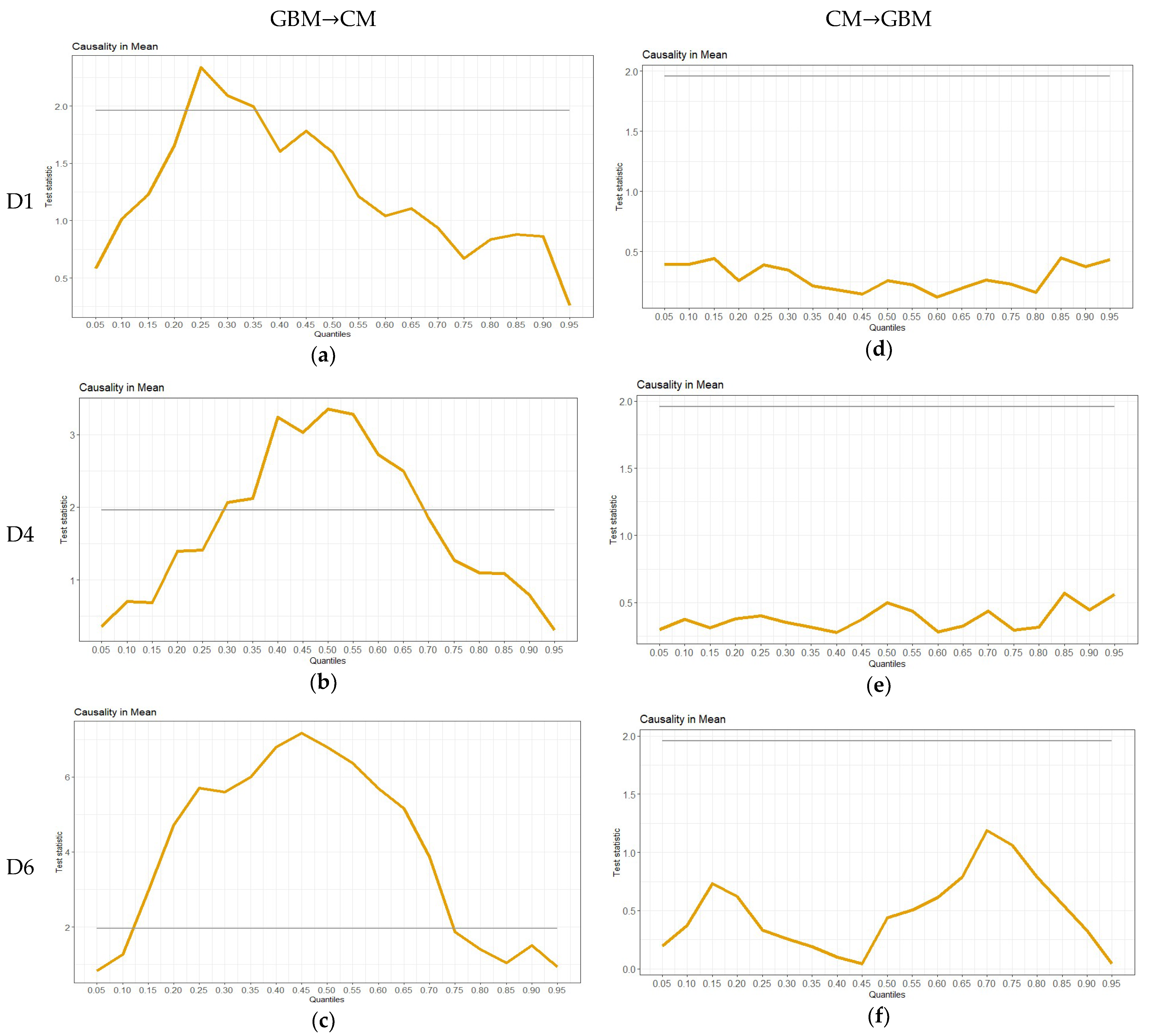
5. Quantile Granger Causality Inference

In order to provide additional clarity regarding the Granger causal relationship between the CM and GBM, we performed a quantile Granger causality test on the MODWT-decomposed sequence. Figure 4 presents the non-parametric Granger average causal relationships at 19 quantiles (ranging from 0.05 to 0.95) within short-term (D1), medium-term (D4), and long-term (D6) time scales—with the gray line indicating the Granger causal relationship at a 5% significance level. As posited by Mensi and Selmi, the position of the quantiles for CM and GBM represents their market performance [25,26], broadly classified into bear markets (q = 0.05 to 0.45), normal markets (q = 0.50), and bull markets (q = 0.55 to 0.95).
Firstly, the Granger causality test of the GBM on the CM (GBMCM)—as depicted in Figure 4a–c—highlights a statistically significant Granger causal relationship between the two markets in the short-term when the quantile range falls between 0.25 and 0.35. For medium- to long-term time scales, a non-smooth inverted U-shaped relationship is detected between the GBM and the CM, indicating that the Granger causal relationship between the two markets is most prominent at the middle quantile position (q = 0.50). Essentially, this implies that under typical market conditions, the GBM has the most substantial impact on the CM.
Furthermore, comparing Figure 4a–c, it is apparent that an increase in time scale expands the quantile range of the GBM with a significant Granger causal relationship on the CM. This suggests that the influence of the GBM on the CM becomes increasingly evident as time goes on. Specifically, in the short term, a Granger causal relationship between the GBM and the CM is observed roughly within the 0.25–0.35 quantile range. In the medium term, this range extends to 0.30–0.70 quantile points, and in the long term, it stretches even further to the 0.15–0.75 quantile range. The findings indicate that although the Granger causal relationship between the GBM and the CM is narrower in range during the short term, it expands gradually over time. Additionally, even under adverse market conditions such as bear and bull markets, the green bond market still exerts a considerable influence on the carbon market.
The results depicted in (d), (e), and (f) of Figure 4 demonstrate that, in the Granger causality test of the CM on the GBM, the threshold of the gray line at the 5% significance level was not surpassed. In simpler terms, the carbon market is unable to effectively forecast the developmental trend of the GBM, irrespective of whether it pertains to the short term, medium term, or long term. These findings demonstrating that green bonds not only deepen the financial market but also contribute to the healthy growth of the carbon market, which is consistent with the study of Yves Rannou (2021) [27]. Consequently, due to the lack of a significant Granger causality relationship between the CM and the GBM, we have plans to undertake a comprehensive investigation on the impact of the GBM on the CM in the future.

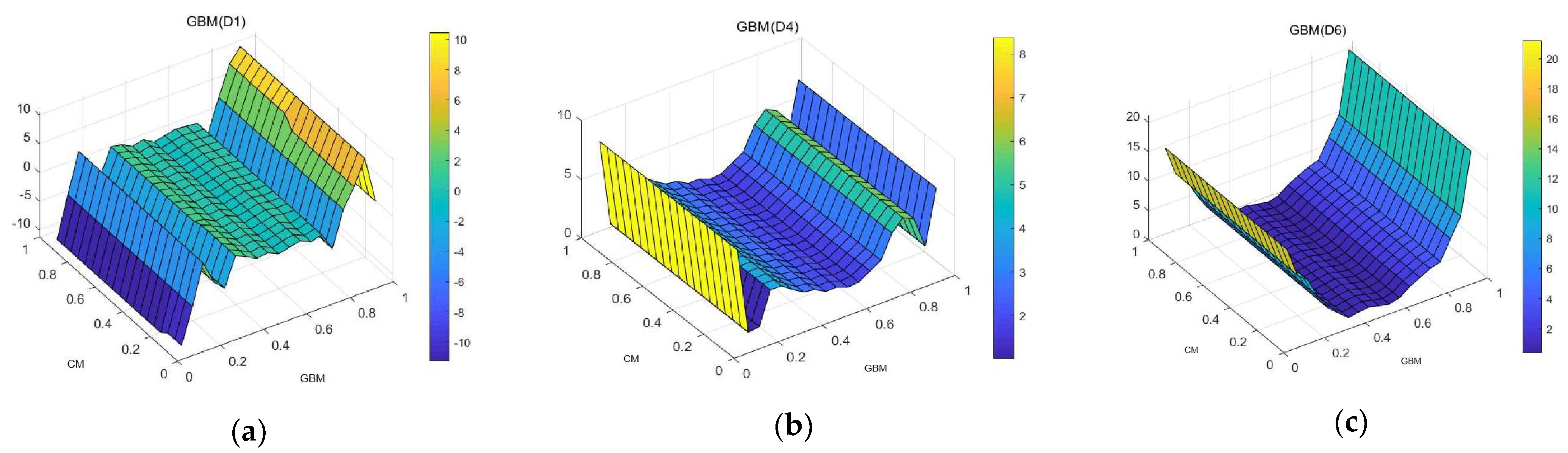
6. Quantile-to-Quantile Regression Results

To comprehensively and systematically comprehend the true impact of the GBM on the CM, this research utilizes the QQR method to investigate the dynamic relationship between the two at three distinct time frames, namely, short term, medium term, and long term. The outcomes are illustrated in (a), (b), and (c) of Figure 5. The main analysis in this study is β 1 ( θ , τ ) , which represents the effect of the θ th quantile of the GBM on the τ th quantile of the CM.
Looking first at the results from the short-term time scale in Figure 5a, β 1 ( θ , τ ) varies with changes in θ , while the effect of the CM quantile τ is relatively small. This implies that the GBM plays a dominant role in the relationship between the CM and the GBM. When the GBM is at a lower quantile ( θ = 0.05 to θ = 0.4), when it is in a “bear market,” it exhibits a strong negative effect on the carbon market. As θ increases, the effect of the GBM on the CM experiences fluctuation in the range of θ = 0.4 to θ = 0.8, with alternating positive and negative effects. Although the favorable impact of the GBM on the CM emerges gradually, it is not consistent. The strongest positive effect of the GBM on the CM is observed when its quantile range falls within 0.85–0.95. Notably, when the GBM is in a “bull market,” this effect is further amplified. Nonetheless, the impacts are somewhat limited. Moreover, when these outcomes are integrated with the Granger causality test outcomes at varying quantiles, it is evident that a statistically significant Granger causality relationship between the CM and the GBM exists at the 0.25–0.30 quantile point within the short-term time frame. Hence, during periods of low activity within the GBM in the short term, it significantly impedes the growth of the CM.
Next, looking at the results of the medium-term time scale in Figure 5b, throughout the quantiles (0.05–0.95), the GBM has a relatively stable and positive dominant effect on the CM ( β 1 ( θ , τ ) fluctuates between 1.156 and 8.384), and this effect exhibits a U-shaped relationship as θ increases. In the medium term, when the GBM increases by one unit, the corresponding increase in the CM fluctuates between 1.156 and 8.384. It is worth noting that when the GBM is at a lower quantile ( θ = 0.05 ), it will have the strongest positive effect on the CM, with β 1 θ , τ = 8.384 ; under this highly optimistic market condition, the result is completely opposite to that under the short-term market condition. As θ gradually increases, when the GBM stabilizes slowly from a sluggish state, after a small peak appears at θ = 0.25 , the positive effect of the GBM on the carbon market gradually decreases, reaching a low point when θ = 0.55 ; at this point β 1 θ , τ = 1.666 . With further increase in θ , after a trough appears at θ = 0.90 , β 1 θ , τ reaches another high point at θ = 0.95 ; at this point β 1 θ , τ = 7.257 . According to the Granger causality test results of the quantiles, the causal relationship between the GBM and the CM is evident at the 0.30–0.70 quantile points. Therefore, in the medium term, the green bond market has a moderate and positive effect on the CM.
Finally, the long-term-scale results in Figure 5c indicate that the GBM still plays a dominant role. A typical U-shaped relationship is observed between the impact of the GBM on the CM across all quantiles, with effect coefficients ranging from 0.370 to 22.227; for every one-unit increase in the GBM, the CM increases by 0.370 to 22.227 units. When θ = 0 .1, the effect of the GBM on the CM is β 1 θ , τ = 15.969 . When θ = 0.55, with β 1 θ , τ = 0.370 , the effect reaches its minimum value. With the further increase of θ , the effect of the GBM on the CM strengthens and reaches its peak at θ = 0.95 with β 1 θ , τ = 21.227 . In the long run, the positive effect of the GBM on the CM stabilizes gradually.
The outcomes indicate that the GBM has a dominant role, irrespective of the considered time horizon. Furthermore, the influence of the GBM on the CM changes from being “restrictive” to “stimulative,” whereby in the short term, when the GBM is lackluster (in the “bear market”), it curbs the growth of the CM [26]. Nevertheless, in the medium and long term, the influence of the GBM on the CM is reasonably favorable for different quantiles. Lastly, in the medium and long term, extreme market conditions in the GBM can cause severe shockwaves. As the quantile θ increases, the impact of the GBM on the CM follows a U-shaped pattern. This U-shaped relationship becomes more prominent with an increase in the time horizon, and this result has also been confirmed by scholars [27,28,29].

7. Robustness Test

7.1. OLS Regression

The OLS regression results are illustrated in Table 3, indicating that during the short-term time frame, the coefficient of GBM on CM is −3.193, which is nonsignificant and suggests that the GBM has a slightly negative impact on the CM in the short term. However, in the medium- and long-term time horizons, the coefficients of GBM are 3.112 and 6.665, respectively, and both pass the 1% significance level test, thereby demonstrating that the GBM has a considerable positive impact on the CM in the medium and long term. These findings not only affirm the robustness of the earlier conclusions but also highlight the inability of the OLS model to capture the asymmetric effects under diverse market conditions and time horizons. As an example, the OLS model fails to reflect the favorable influence of GBM on CM in the short term, suggesting that the QQR method is more suited for analyzing complex and diverse issues by exposing the connection between the GBM and the CM at various combined quantiles.

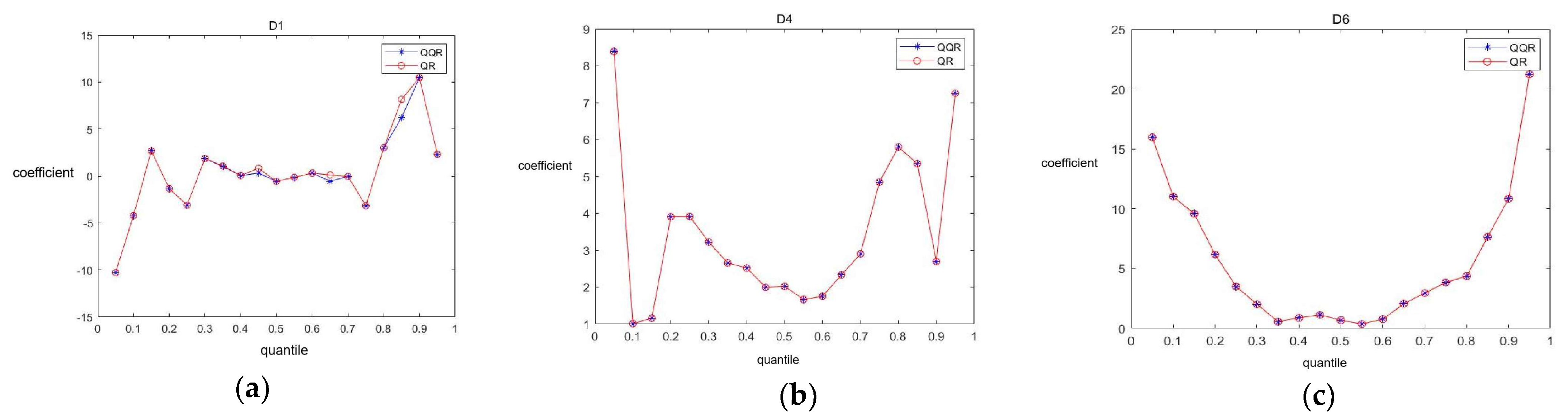
7.2. Comparison of Regression Coefficient between QQR and QR

To further verify the robustness of the research results mentioned above, this paper compares the QR coefficient with the τ -average coefficient of QQR. The formula for calculating the τ -average coefficient is as follows:
γ 0 ( θ ) β ^ ^ 0 ( θ ) = 1 D τ β ^ 0 ( θ , τ )
γ 1 ( θ ) β ^ ^ 1 ( θ ) = 1 D τ β ^ 1 ( θ , τ )
In the above equation, D is the number of grid points for τ , that is, D = 19. Figure 6a, 6b, and 6c, respectively, show the coefficient curves of QQR and QR on short-term, medium-term, and long-term time horizons. From the perspective of the short-term time horizon, there is a deviation between the coefficients of QQR and QR at the 0.45, 0.65, and 0.85 quantiles. The reason for the deviation in the results of QQR and QR in the short term may be due to the interference of noise caused by some short-term unexpected events. However, the sequence becomes more stable in the medium- and long-term time horizons, and the results of QQR are consistent with those of QR. Therefore, the above results indicate the robustness of the research conclusions mentioned above.

8. Conclusions and Suggestions

To explore the correlation effect between the GBM and CM, daily frequency time series data from 9 August 2013, to 29 June 2022, are selected as the original sequence. Then, the MODWT is used to generate the basic research sequence. Subsequently, the quantile Granger causality test and QQR method are utilized to analyze the causal relationship and the effects of the two markets at short-, medium-, and long-term time horizons. The following research findings are obtained:
First, utilizing the quantile Granger causality test, it is established that a statistically significant Granger causality relationship exists between the CM and the GBM, regardless of the market conditions and time horizon. Meanwhile, the GBM demonstrates a discernible causal association with the CM, which becomes more noticeable as the time horizon expands. This implies that the one-way connection between the GBM and the CM becomes more apparent as time progresses.
Second, the GBM plays a prevailing role in both markets. During a bear market phase, the green bond market can negatively affect the CM in the short term. However, it exerts a positive impact on the CM in the medium- to long-term time horizons. Moreover, as the time horizon extends, the synergies between the GBM and the CM become more apparent. In the medium to long term, severe market conditions can lead to a remarkable impact of the GBM on the CM.
Based on the research findings above, we propose the following policy recommendations:
Firstly, policymakers should consider the interrelated effects between the two markets when formulating policies and timely implement corresponding measures. In the short term, attention should be paid to preventing risk contagion between the markets under extreme market conditions; in the long term, risk contagion under normal market conditions should be prevented to maximize the synergistic promotion effect of the CM and the GBM. In addition, the carbon market trading system should be further improved by introducing carbon emission quota auctions to increase carbon prices. The price constraint mechanism of the CM should be fully utilized to guide energy transformation and promote the development of the green industry. Secondly, for CM investors, investment portfolios and risk mitigation strategies should be adjusted according to market changes to maximize investment returns. Thirdly, for companies engaged in emission control, given the similarity between the GBM and the CM, issuing more green bonds to fund their low-carbon transformation projects can help them achieve their emission reduction targets and minimize their reliance on the carbon market.

9. Limitations and Future Research

First, due to the reality of China’s unique national conditions, there are still many influencing factors in the relationship between the carbon market and the green bond market, so future research should further analyze the influencing factors of their correlation characteristics. Second, the indicators of the carbon market and the green bond market adopted in this study are still immature, and a more reasonable indicator system should be analyzed in the future. Third, there is still significant room for improvement in the economic reasons behind the results and more appropriate policy measures, which will be a major focus of our future research.

Author Contributions

D.W.: data curation, formal analysis, writing, and supervision; Z.L.: data curation and software; T.Z.: data curation, formal analysis, and writing; L.T.: data curation and software; M.A.: data curation and software; X.F.: data curation, formal analysis, and writing. All authors have read and agreed to the published version of the manuscript.

Funding

This research received no external funding.

Institutional Review Board Statement

Not applicable.

Informed Consent Statement

Not applicable.

Data Availability Statement

The data used in this article come from a study conducted in 2022.

Acknowledgments

Many thanks to Ding Wu for their guidance on this article.

Conflicts of Interest

The authors declare no conflict of interest.

References

  1. Palao, F.; Pardo, A. Assessing price clustering in European carbon markets. Appl. Energy 2012, 92, 51–56. [Google Scholar] [CrossRef]
  2. Liu, M. The driving forces of green bond market volatility and the response of the market to the COVID-19 pandemic. Econ. Anal. Policy 2022, 75, 288–309. [Google Scholar] [CrossRef]
  3. Lin, B.; Huang, C. Analysis of emission reduction effects of carbon trading: Market mechanism or government intervention? Sustain. Prod. Consum. 2022, 33, 28–37. [Google Scholar] [CrossRef]
  4. Flammer, C. Corporate green bonds. J. Financ. Econ. 2021, 142, 499–516. [Google Scholar] [CrossRef]
  5. Reboredo, J.C. Green bond and financial markets: Co-movement, diversification and price spillover effects. Energy Econ. 2018, 74, 38–50. [Google Scholar] [CrossRef]
  6. Pham, L. Frequency connectedness and cross-quantile dependence between green bond and green equity markets. Energy Econ. 2021, 98, 105257. [Google Scholar] [CrossRef]
  7. Fan, Y.; Jia, J.-J.; Wang, X.; Xu, J.-H. What policy adjustments in the EU ETS truly affected the carbon prices? Energy Policy 2017, 103, 145–164. [Google Scholar] [CrossRef]
  8. Ren, X.; Dou, Y.; Dong, K.; Li, Y. Information spillover and market connectedness: Multi-scale quantile-on-quantile analysis of the crude oil and carbon markets. Appl. Econ. 2022, 54, 4465–4485. [Google Scholar] [CrossRef]
  9. Mansanet-Bataller, M.; Soriano, P. Volatility transmission in the CO2 and energy markets. In Proceedings of the 6th International Conference on the European Energy Market, Leuven, Belgium, 27–29 May 2009; pp. 1–7. [Google Scholar]
  10. Chen, Y.; Qu, F.; Li, W.; Chen, M. Volatility spillover and dynamic correlation between the carbon market and energy markets. J. Bus. Econ. Manag. 2019, 20, 979–999. [Google Scholar] [CrossRef] [Green Version]
  11. Reboredo, J.C. Volatility spillovers between the oil market and the European Union carbon emission market. Econ. Model. 2014, 36, 229–234. [Google Scholar] [CrossRef]
  12. Mol, A.P.J. Carbon flows, financial markets and climate change mitigation. Environ. Dev. 2012, 1, 10–24. [Google Scholar] [CrossRef]
  13. Liu, Z.; Zhang, Y.-X. Assessing the maturity of China’s seven carbon trading pilots. Adv. Clim. Chang. Res. 2019, 10, 150–157. [Google Scholar] [CrossRef]
  14. Lin, B.; Chen, Y. Carbon price in China: A CO2 abatement cost of wind power perspective. Emerg. Mark. Financ. Trade 2018, 54, 1653–1671. [Google Scholar] [CrossRef]
  15. Fan, X.; Li, X.; Yin, J.; Tian, L.; Liang, J. Similarity and heterogeneity of price dynamics across China’s regional carbon markets: A visibility graph network approach. Appl. Energy 2019, 235, 739–746. [Google Scholar] [CrossRef]
  16. Das, D.; Kannadhasan, M. Do global factors impact bitcoin prices? Evidence from wavelet approach. J. Econ. Res. 2018, 23, 227–264. [Google Scholar]
  17. Mishra, S.; Sharif, A.; Khuntia, S.; Meo, M.S.; Khan, S.A.R. Does oil prices impede Islamic stock indices? Fresh insights from wavelet-based quantile-on-quantile approach. Resour. Policy 2019, 62, 292–304. [Google Scholar] [CrossRef]
  18. Koenker, R.; Xiao, Z. Unit root quantile autoregression inference. J. Am. Stat. Assoc. 2004, 99, 775–787. [Google Scholar] [CrossRef] [Green Version]
  19. Galvao, A.F., Jr. Unit root quantile autoregression testing using covariates. J. Econom. 2009, 152, 165–178. [Google Scholar] [CrossRef]
  20. Jeong, K.; Härdle, W.K.; Song, S. A consistent nonparametric test for causality in quantile. Econom. Theory 2012, 28, 861–887. [Google Scholar] [CrossRef] [Green Version]
  21. Troster, V. Testing for Granger-causality in quantiles. Econom. Rev. 2018, 37, 850–866. [Google Scholar] [CrossRef]
  22. Sim, N.; Zhou, H. Oil prices, US stock return, and the dependence between their quantiles. J. Bank. Financ. 2015, 55, 1–8. [Google Scholar] [CrossRef]
  23. Ren, X.; Lu, Z.; Cheng, C.; Shi, Y.; Shen, J. On dynamic linkages of the state natural gas markets in the USA: Evidence from an empirical spatio-temporal network quantile analysis. Energy Econ. 2019, 80, 234–252. [Google Scholar] [CrossRef]
  24. Wen, F.; Shui, A.; Cheng, Y.; Gong, X. Monetary policy uncertainty and stock returns in G7 and BRICS countries: A quantile-on-quantile approach. Int. Rev. Econ. Financ. 2022, 78, 457–482. [Google Scholar] [CrossRef]
  25. Mensi, W.; Hammoudeh, S.; Tiwari, A.K. New evidence on hedges and safe havens for Gulf stock markets using the wavelet-based quantile. Emerg. Mark. Rev. 2016, 28, 155–183. [Google Scholar] [CrossRef]
  26. Selmi, R.; Mensi, W.; Hammoudeh, S.; Bouoiyour, J. Is Bitcoin a hedge, a safe haven or a diversifier for oil price movements? A comparison with gold. Energy Econ. 2018, 74, 787–801. [Google Scholar] [CrossRef]
  27. Rannou, Y.; Boutabba, M.A.; Barneto, P. Are Green Bond and Carbon Markets in Europe complements or substitutes? Insights from the activity of power firms. Energy Econ. 2021, 104, 105651. [Google Scholar] [CrossRef]
  28. Ahmad, M.; Ahmed, Z.; Khan, S.A.; Alvarado, R. Towards environmental sustainability in E−7 countries: Assessing the roles of natural resources, economic growth, country risk, and energy transition. Resour. Policy 2023, 82, 103486. [Google Scholar] [CrossRef]
  29. Ahmad, M.; Ahmed, Z.; Yang, X.; Can, M. Natural Resources Depletion, Financial Risk, and Human Well-Being: What is the Role of Green Innovation and Economic Globalization? Soc. Indic. Res. 2023, 167, 269–288. [Google Scholar] [CrossRef]
Figure 1. Carbon market and green bond market time series graph.
Sustainability 15 10634 g001
Figure 2. Nuclear density estimates for carbon markets and green bond markets.
Sustainability 15 10634 g002
Figure 3. MODWT chart of carbon market and green bond market.
Sustainability 15 10634 g003aSustainability 15 10634 g003b
Figure 4. Quantile Granger causality inference. Note: The gray lines represent T-values at the 5% significance level.
Sustainability 15 10634 g004
Figure 5. Quantile-to-quantile regression results.
Sustainability 15 10634 g005
Figure 6. QR and QQR regression coefficient comparison.
Sustainability 15 10634 g006
Table 1. Descriptive statistics and JB test.
CMGBM
Obs18081808
Mean0.00040.0003
Minimum−1.891−0.008
25% quantile−0.066−0.0001
75% quantile0.0680.0006
Maximum1.9640.193
Std.Dev0.2040.001
Skewness0.3392.411
Kurtosis27.95452.174
Jarque–Bera test46,943.147 ***183,916.170 ***
Note: Bold font in the text indicates data with special characteristics, which are retained to four decimal places for distinction. The significance levels are denoted by ***, which correspond to 10%, 5%, and 1%, respectively.
Table 2. Quantile unit root test.
GBMCM
Quantile α τ T-ValueCV α τ T-ValueCV
0.050.297−7.093−3.279 −0.367−14.301−2.310
0.10.371−15.273−3.317 −0.351−31.837−2.553
0.150.368−22.250−3.355 −0.307−49.3862−2.468
0.200.380−30.440−3.401 −0.275−60.670−2.638
0.250.375−34.513−3.337 −0.265−66.040−2.732
0.300.370−39.352−3.327 −0.258−72.014−2.832
0.350.374−42.826−3.269 −0.250−75.923−2.847
0.400.382−43.830−3.272 −0.262−80.462−2.927
0.450.382−46.104−3.237 −0.267−85.669−2.896
0.500.386−46.3145−3.287 −0.252−86.437−2.852
0.550.402−45.566−3.238 −0.255−88.133−2.801
0.600.408−42.313−3.193 −0.271−93.759−2.760
0.650.420−38.819−3.116 −0.265−84.966−2.757
0.700.435−32.769−3.074 −0.262−80.750−2.582
0.750.434−29.072−3.046 −0.250−71.484−2.510
0.800.409−26.190−2.971 −0.279−60.926−2.310
0.850.406−21.589−2.922 −0.309−44.966−2.310
0.900.431−15.227−2.755 −0.333−29.725−2.310
0.950.382−7.128−2.486 −0.424−16.049−2.510
Note: CV represents a critical value of 5% significance.
Table 3. OLS regression results.
Short-TermMedium-TermLong-Term
CMCMCM
GBM−3.1933.112 **6.665 ***
(−0.50)(2.16)(7.75)
_cons−0.0000.0000.000
(−0.00)(0.00)(0.00)
N180818081808
Note: ** means p < 0.05, *** means p < 0.01, and the T value is in parentheses.
Disclaimer/Publisher’s Note: The statements, opinions and data contained in all publications are solely those of the individual author(s) and contributor(s) and not of MDPI and/or the editor(s). MDPI and/or the editor(s) disclaim responsibility for any injury to people or property resulting from any ideas, methods, instructions or products referred to in the content.

