Article

Regulation and Optimization of Urban Water and Land Resources Utilization for Low Carbon Development: A Case Study of Tianjin, China

1
School of Economics and Management, Hebei University of Technology, Tianjin 300401, China
2
Tianjin Academy of Eco-Environmental Sciences, Tianjin 300191, China
*
Author to whom correspondence should be addressed.
Sustainability 2022, 14(5), 2760; https://doi.org/10.3390/su14052760
Submission received: 26 January 2022 / Revised: 23 February 2022 / Accepted: 24 February 2022 / Published: 26 February 2022

Abstract

:
The consumption of energy and resources produces carbon emissions and exacerbates global warming. As the basic resources for urban development, the development and utilization of water and land resources consume a large amount of energy, which results in carbon emissions. This paper presents a study aimed at analyzing the interaction of urban water–land–energy and its carbon emission effects and finding ways to achieve the win-win situation of carbon emission reduction and economic development. We used an SD-MOP model combined with system dynamics (SD) and multi-objective programming (MOP) to describe the feedback relationship between urban water and land resources utilization and carbon emissions, designed a comprehensive scheme for carbon emission reduction goal and optimized it in order to achieve the low carbon development goal. Tianjin, one of the four province-level municipalities, was investigated as a case study for this research. The simulation results indicate that Tianjin’s carbon emissions from water and land utilization will peak around 2025 when applying the comprehensive regulation scheme. After optimization, the optimal regulation scheme would achieve considerable social, economic and environmental benefits. We suggest the implementation of measures including the optimization of the industrial, energy and land use structure; the improvement of energy efficiency; increasing residents’ low carbon awareness; and strengthening industrial and domestic water savings to realize the low carbon development of the city. The findings of this study will be useful for the management of urban water and land utilization.

1. Introduction

Carbon emissions are a main cause of the global temperature rise witnessed over the past 100 years [1]. The global CO2 concentration increased from 227 ppm in 1750 to 409.85 ppm in 2019. About 81% of total carbon emissions came from fossil fuel combustion and 19% came from land use change [2]. A series of problems caused by global warming pose challenges to the survival and development of human society. As a country with the largest carbon emissions in the world, the Chinese government promised at the Paris Climate Change Conference in 2015 that carbon dioxide emissions would peak around 2030 and that the carbon dioxide emissions per unit of GDP at this time would be 60–65% lower than they were in 2005. In 2020, the Chinese government promised the world a new goal, which was to strive to achieve carbon neutrality by 2060 [3]. Facing the commitments made by the Chinese government to the world, how to achieve the emission reduction goal while maintaining economic growth, which is the path to low-carbon development is an important issue that policymakers should consider.
The utilization of natural resources consumes energy and generates carbon emissions. With a large number of industries and residents, the city is not only the main contributor to energy consumption and greenhouse gas emissions, but also a critical region where carbon emission reduction action needs to be considered. Land resource is the spatial carrier of the city, and land use change affects industrial and population distribution, which in turn affects energy consumption and carbon emissions [2]. Water resources are the limiting factor for urban development, and their quantity and quality determine urban population growth, urbanization level, and industrial development patterns. Urban water production and treatment consume a lot of energy, resulting in carbon emissions. Meanwhile, the utilization modes of water and land resources also change the habitats of biota and affect the biological health status [4,5], ultimately affecting urban development and human survival. In 2012, the U.S. Department of Energy [6] systematically analyzed the carbon emissions of water and land resources utilization, which is a new approach to carbon emission research. Zhao et al. [7] introduced this idea into China and carried out empirical research. China’s development is facing resource and environmental pressures, and the problem of carbon emissions from the utilization of water and land resources has been attracting more and more attention.
Research in the field of water and land resources for low carbon development began to appear around 2000. The research objective has changed from the initial single element to all water and land resources over the years. In the field of water resource, the research focuses on issues such as the coupling of crop water, energy and carbon flux [8,9]; carbon emissions of regional water resource development and utilization [10,11]; and carbon and water resource planning [12]. In the field of land resource, early studies focused on the impact of land use change on soil carbon flux [13] and natural ecosystem carbon balance [14]. In recent years, the area of study has expanded to the relationship between land use, energy consumption and carbon budget [15,16], and land use regulation for the low carbon goals [17]. Recently, more and more scholars have come to the realization that water resources and land resources are interrelated and mutual resources in different ways and constitute the resource base of regional social and economic development, with the two being impossible to completely separate. Therefore, the research has gradually expanded from focusing on a single element to considering the interaction between water and land resources as a whole and their interaction with other elements such as energy and carbon emissions. In terms of the coupling effect of water and land resources, energy, and carbon emissions, Skaggs et al. [6] explored the mechanism of climate change from a new perspective—through the coupling of water and land resources’ development and utilization, energy inputs, and carbon emissions. They took the United States as an example to analyze the role of the energy–water–land system in climate change mitigation and adaptation. Then, different scholars studied agricultural carbon emissions in different regions from this perspective. For example, Zhao et al. [7] found the ratio of water to land resources can promote or inhibit agricultural carbon emissions in different provinces in China. Some scholars have carried out research from the perspective of carbon footprints [18,19], and proposed a comprehensive analysis method that combines the ecological footprint, energy footprint, carbon footprint and water footprint. In addition, some scholars [20] used an energy analysis method to research the impact of land use change on carbon water ecosystem services in sparse grassland areas, and found that the carbon water ecosystem service function under traditional farming methods is the lowest.
At present, most studies on the regulation of water and land resources are carried out in the form of resource planning and allocation. The regulation goal has changed from maximizing the benefits of water and land supply to seeking benefits for society, the economy, resource balance, and the environment. This change shows that human beings constantly reflect on the impact of their own behavior on the natural environment and pursue the sustainable development of both human society and nature. The research into water resource allocation began in the mid-20th century with the reservoir optimal scheduling problem, then the research objective extended from the reservoir or irrigation area to regions [21], watersheds [22], and cities [23]. The allocation goal has changed from only focusing on the benefits of water use to pursuing comprehensive benefits to the economy, society and the ecological environment. Studies of land resource allocation have been produced and enriched with the establishment of land systems and the development of land system reform all over the world. In recent years, based on the status quo of social and economic development, scholars have used a variety of methods to study land use allocation and land management modes at different scales, including watersheds [24], cities [25] and industry [26], and the allocation goals have gradually diversified. If only single element allocation is carried out, it may have an adverse effect on the comprehensive utilization of resources. Scholars have gradually realized that joint allocation of water and land resources should be conducted. The early research mainly focused on the joint allocation of water and land resources in irrigation areas [27]. After 2000, the research objectives expanded to multiple scales such as regions [28] and watersheds [29]. The research contents and methods were gradually enriched, and the allocation objectives were transformed from single objectives to multiple objectives. Other scholars [30] have paid attention to the role of water resources in transnational land investment, and found that the potential of rainfed crop production in target areas and the abundance of land resources are important driving factors for transnational land investment.
The system engineering method is the main method for water and land resource regulation, including the linear programming model, the MOP model, the SD model, etc. The linear programming model calculates the optimal solution of water and land resources regulation that meets the constraints and objectives. Das et al. [31] used the linear programming model to study the optimal allocation of water and land resources in irrigation areas of the United States and India with the goal of maximizing the net income of crops. With the evolution of the regulation objectives for water and land resources to the comprehensive coordination of economic, social and ecological benefits, the application of the MOP model is becoming widespread. The multiple objectives of water and land resources regulation usually include economic objectives such as the economic output of water resources [32] and land use benefits [33]; social objectives, such as water consumption satisfaction [32] and the land use intensity level [34]; and environmental objectives, such as water pollutant discharge [35], forest coverage [36], ecosystem services [37], and carbon emissions [38]. The SD model has the advantages of simulating the dynamic process of the system and solving nonlinear and complex time-varying system problems. Since the regulation of water and land resources involves feedback among multiple subsystems such as the water and land resources system and the socioeconomic system, the SD model has been more and more widely used in related research in recent years [39,40,41]. However, the SD model has no advantages in multi-objective optimization. Consequently, some scholars combine it with other models, such as the SD-MOP integration model, which combines the SD model with the MOP model, to study urban resource planning [42], but research in this area is scarce [43].
Through a literature review, we found that the existing research has the following two shortcomings. First, it does not explore the impact of human activities on urban carbon emissions from the perspective of resource development and utilization or the coupling mechanism of water and land resource development and utilization, energy input, economic development, population growth, and carbon emissions. Second, there are few studies on the comprehensive regulation of water and land resources for low carbon development goals using multiple methods. In this paper, we adopt the SD-MOP model, which establishes a MOP model considering economic, social, and environmental benefits on the basis of identifying important decision variables of the SD model, to study the low carbon development of urban water and land resources utilization. The NSGA-II algorithm is used to solve the MOP problem and the technique for order preference, similar to an ideal solution and analytic hierarchy process integrated model (TOPSIS-AHP), is used to choose the optimal solution. Then, the urban low carbon water and land resources utilization scheme considering multi-objectives is obtained, which will be useful for the management of urban water and land utilization. This paper makes three contributions. First, it constructs a conceptual model of urban water and land resources regulation for low carbon development and clarifies the coupling mechanism of urban water and land resource utilization and carbon emissions. Second, this paper builds a carbon emission system dynamics model of urban water and land resources utilization composed of five subsystems, including population, economy, energy, water resource utilization and land use, designs the regulation schemes to observe the changes of output variables, and selects the optimal scheme. Third, this paper builds a MOP model including multi-objectives from the aspects of society, economy, and environment to further optimize the allocation of water and land resources of the selected scheme, finally obtaining the optimal urban water and land resources utilization scheme in line with the goal of low carbon development.

2. Methods and Data

2.1. The Regulation Mechanism of Urban Water and Land Resources Utilization for Low Carbon Development

Learning from the theories proposed by Skaggs et al. [6] and Zhao et al. [7], we put forward the regulation mechanism of urban water and land resources utilization for low carbon development, which consists of three key elements: water, land, and energy. Water resources are necessary for the survival of urban residents, animals, and plants and provide raw materials and production conditions for the production processes of various industries. Land resources provide physical places for urban human activities, the survival of animals and plants, industrial production, transportation, and other socioeconomic activities, and also provide the means of production for agriculture. Energy provides a source of power for various socioeconomic activities. The development and utilization of water, land and energy interact with each other and produce carbon emissions. Carbon emissions are not only the metabolites of the interaction of the three elements, but also the external environmental effects produced by the interaction.
The conceptual model of urban water and land resources utilization and regulation mechanism for low carbon development is shown in Figure 1. Activities of water resource utilization, land use and energy development and utilization are the main elements of the system and are also the resource basis of urban socioeconomic development. Water resource utilization includes the whole life cycle of water resource utilization, including water intake, water production, water delivery, water use, and water treatment. Land use includes agricultural production activities on agricultural land, construction activities on construction land and other land resource development and utilization activities. Energy development and utilization include energy extraction, processing, transportation and consumption. Water, land, and energy are coupled and influenced by supply and demand relationships, forming a variety of complex feedback loops and interactions through the water–land relationship, the land–energy relationship, and the water–energy relationship. The water cycle, land use activities, energy flow, and the carbon cycle constitute the main contents of urban equilibria, and are affected by external factors such as socioeconomic development, resource endowment, technical progress, government regulation and the social environment, which are continuously in the process of dynamic evolution. The regulation goal is to realize urban low carbon development, intensive utilization of natural resources, and sustainable socioeconomic development in order to finally achieve a harmonious coexistence between human society and nature.

2.2. SD-MOP Model

The SD-MOP model combines the SD model with the MOP model and is a planning decision support method that has emerged in the past ten years [44]. The SD model can easily and flexibly conduct decision-making simulations and multi-scheme comparisons and is suitable for studying the structural function coordination of complex systems and the dynamic development of medium and long-term systems. It focuses on the long-term, comprehensive description of system behaviors and trends. However, some parameters in the model are difficult to quantify accurately, and the answer provided is often not the optimal solution. The MOP model is suitable for solving the problem from a definite and static viewpoint and can find the optimal solution of the parameters, but it is difficult to examine the comprehensive dynamic process of the system. The SD-MOP model overcomes the limitations of the two models, which can fully reflect the trend of system development, and precisely describes the structure and function of the system. The carbon emissions of urban water and land resource utilization are influenced by many factors, and there is a feedback relationship between each element of the system; thus it can be simulated with the SD model. Moreover, low-carbon development should yield a win-win situation in terms of low carbon development. Urban managers need to consider multiple objectives that are contradictory and irreducible when regulating water and land resources, which is why the MOP model needs to be used simultaneously. Therefore, this paper selected the SD-MOP model to seek the optimal scheme.
The modeling steps of the SD-MOP model are shown in Figure 2 and described as follows:
(1)
On the basis of conducting a system analysis, the SD model is established to simulate the system development. Then, the key decision variables that have a greater impact on the system are identified through the sensitivity analysis and system running.
(2)
Taking the key decision variables as independent variables, the objective functions and constraints are used to build a MOP model. An appropriate method is chosen to solve the model and obtain the optimal values of the key decision variables.
(3)
The optimal values of the key decision variables are fed into the SD model, the model is run and the simulation results are analyzed. Then, the MOP model is adjusted according to the decision requirements. Finally, a satisfied optimal decision scheme is found.

2.3. SD Model and Regulation Scheme Design

The SD model of carbon emissions for urban water and land resources utilization composed of the land use subsystem, the water resource utilization subsystem, the economic subsystem, the population subsystem and the energy consumption subsystem was established using Vensim. The causal loop diagram of the system is shown in Figure 3.
The land use subsystem involves the agricultural production activities on farmland (including arable land, forest land, garden land, grassland, and other farmland), the development and construction activities on construction land (including residential and industrial land, transportation land, and water conservancy facilities land), as well as the land use carbon sink of arable land, forest land, garden land, grassland area and unused land. The water resource utilization subsystem involves the service activities of each phase of the municipal water system (including water supply, water use, and water treatment). The economic subsystem includes the urban economic development speed and industrial structure. The population subsystem includes the total population, urban population and rural population. The energy consumption subsystem includes the industrial and household energy consumption. The main variables of each subsystem are shown in Table 1.
After the model is established, a running test, historical test and sensitivity analysis needed to be performed to ensure that the model could meet the running conditions and could be used to simulate the carbon emissions of urban water and land resources utilization. Then, we selected variables from the subsystems, and designed the comprehensive regulation schemes for carbon emission reduction.

2.4. Mop Model and Regulation Scheme Optimization

2.4.1. Key Decision Variables Identification

Considering that the allocation area of each land type in the regulation schemes is set artificially, it is difficult to reach the optimal solution. Meanwhile, since water resource is the limiting factor of urban development and plays a bottom-line role in maintaining the operation of the city, thus we selected the parameters with high sensitivity from the land use and water resource utilization subsystems as the key decision variables, and optimized them with the MOP model.

2.4.2. Objective Function Establishment

The regulation of urban water and land resources utilization for low carbon development needs to achieve multi-objective coordination, which means the city can obtain more development opportunities while meeting carbon emission reduction targets. Water and land resources, as the basic resources supporting urban development, should meet the needs of urban development under the premise of intensive utilization. The values of other parameters in the MOP model except the key decision variables equal the values in the SD model. Accordingly, this paper established the following three objective functions consisting of social, economic and environmental benefits.
The objective function of social benefit is to minimize the total water demand, and can be expressed as follows:
M i n F 1 = y x g g + q n + q s + i = 1 2 p c i d c i + m = 1 3 j g m y g m
where F 1 is the total water demand; y x is the size of irrigated area; g g is the irrigation water demand per unit area; q n is the other water demand of agriculture; q s is the ecological water demand; p c i is the population; d c i is the per capita domestic water demand; i = 1 , 2 represents urban and rural areas, respectively; j g m is the manufacturing industry GDP; y g m is the water demand per unit GDP; m = 1 , 2 , 3 represents manufacturing industry, construction industry and tertiary industry, respectively.
The objective function of economic benefit is to maximize the total GDP, and can be formulated as follows:
M a x F 2 = y c × n = 1 4 n d n + ( e c + f c ) × j = 1 3 j s j
where F 2 is the total GDP; y c is the agriculture GDP per unit farmland area; n d n is the area of each type of farmland; n = 1 , 2 , 3 , 4 represents the arable land area, garden land area, forest land area, and other farmland area, respectively; e c is the secondary industry GDP per unit construction land area; f c is the tertiary industry GDP per unit construction land area; j s j is the area of each type of construction land; j = 1 , 2 , 3 represents residential and industrial land area, traffic land area and water conservancy facilities land area, respectively.
The objective function of environmental benefit is to minimize the net carbon emissions of urban water and land resources utilization, and can be calculated as follows:
M i n F 3 = c t + n d 1 ( g t g h ) + n d 4 o t j s 3 s h + k = 1 4 y s k p f k + j = 1 2 j s j j t j n = 2 3 n d n l h n
where F 3 is the net carbon emissions of urban water and land resources utilization; c t is the carbon emissions of water supply and sewage treatment; g t is the carbon emission intensity per unit arable land area; g h is the carbon sink intensity per unit arable land area; o t is the carbon emission intensity per unit other farmland area; s h is the carbon sink intensity per unit water conservancy facilities land area; y s k is the water demand; p f k is the carbon emission intensity per unit water consumption; k = 1 , 2 , 3 , 4 represents agriculture, secondary industry, tertiary industry and household, respectively; j t j is the carbon emission intensity per unit residential and industrial land area/traffic land area; l h n is the carbon sink intensity per unit garden land/forest land area.

2.4.3. Constraint Conditions Determination

According to urban land use planning, water supply and water use planning, we selected parameters related to water and land resources allocation in the SD model and set parameter constraints.
The water resource and land resource constraint conditions can be expressed as follows:
G G max y x g g G G min
S H max i = 1 2 p c i d c i S H min
C Y max m = 1 3 j g m y g m C Y min
N D max n = 1 4 n d n N D min
J S max j = 1 3 j s j J S min
where G G max and G G min represent the maximum and minimum of irrigation water demand; S H max and S H min represent the maximum and minimum of domestic water demand; C Y max and C Y min represent the maximum and minimum of manufacturing water demand; N D max and N D min represent the maximum and minimum of farmland area; J S max and J S min represent the maximum and minimum of construction land area.

2.4.4. Optimal Solution to the MOP Model

The classical MOP model is usually solved by transforming the multi-objective problem to a single objective problem through objective weighting, objective programming and ε –constraint method, for which some parameters need to be manually specified, resulting in strong subjectivity and unsatisfactory optimization results. In recent years, scholars began to use intelligent algorithms to solve the MOP problem, which reduces the subjective impact on solutions and improves the solution accuracy. The genetic algorithm is one of the intelligent algorithms suggested by Holland in 1975. Based on the evolutionary principle of “survival of the fittest”, the solution of the problem is expressed as “chromosome”. Through the evolution of chromosomes, a better individual, that is, the optimal solution of the problem, is finally obtained. Due to the high parallelism and global search ability, the genetic algorithm has been widely used in solving MOP problems. Of them, NSGA-II, PESA-II and SPEA-II enjoyed more attention and have been widely used in engineering and scientific fields [45,46,47]. PESA-II algorithm has good astringency especially when solving high-dimensional optimization problems, but the selection takes a long time and has poor diversity. SPEA-II algorithm has the advantage in solving high-dimensional optimization problems, and can obtain uniformly distributed Pareto-optimal solutions, but the clustering process is time-consuming and inefficient. The NSGA-II algorithm has high efficiency and good solution distribution [44], which is suitable for low-dimensional MOP problems. Our study has three objective functions; thus the NSGA-II algorithm can be used to solve the MOP problem.
The NSGA-II algorithm includes the following steps: initially, an initial random parent population of size N is generated. Fast, non-dominated sorting is assumed and a first offspring population of size N is created through the usual selection, crossover, and mutation operators. Then, starting from the second generation, the parent population and the offspring population are combined to obtain a population of size 2N. Then, the combined population is subjected to fast, non-dominated sorting and crowding distance calculation, and appropriate individuals are selected to form a new parent population of size N. Finally, a new offspring population is generated through using the usual population operators of the genetic algorithm. The loop will stop until the maximum evolutionary algebra is reached, and the Pareto-optimal solutions will be output.
The solution of the MOP problem is divided into two steps. One is to use the NSGA-II algorithm to obtain the Pareto-optimal solutions; the other is to find an optimal decision scheme from Pareto-optimal solutions, which is determined by using a combination method of TOPSIS and AHP. The TOPSIS method selects the solution with the shortest distance from the positive ideal solution and the farthest distance from the negative ideal solution as the optimal decision scheme. It has the advantages of robust logical structure, simple calculation process and considering both the positive and negative ideal solutions at the same time. The AHP method is assumed to calculate the weight of each objective and is one of the input parameters for the TOPSIS. The decision-making steps of the TOPSIS-AHP method are as follows:
  • Constructing the normalized initial matrix.
Assuming there are n Pareto-optimal solutions and each solution has m attributes, the initial matrix is constructed as:
X = [ x 11 x 12 x 1 m x 21 x 22 x 2 m x n 1 x n 2 x n m ]
Creating the weighted normalization matrix, and the attributes are vector normalized. The formula is shown in Equation (10) and the normalized matrix Z is obtained.
z i j = x i j i = 1 n x i j 2
2.
Determining the positive and negative solutions.
For the optimization problem whose purpose is to minimize the objective function, the positive ideal solution ( Z + ) is composed of the minimum value of each column, and the negative ideal solution ( Z ) is composed of the maximum value of each column.
Z + = ( max { z 11 , z 21 , , z n 1 } , max { z 12 , z 22 , , z n 2 } , , max { z 1 m , z 2 m , , z n m } ) = ( Z 1 + , Z 2 + , , Z m + )
Z = ( min { z 11 , z 21 , , z n 1 } , max { z 12 , z 22 , , z n 2 } , , max { z 1 m , z 2 m , , z n m } ) = ( Z 1 , Z 2 , , Z m )
3.
Setting weights of objective functions.
First, experts are invited to score the relative importance of pairwise attributes. The score of relative importance takes a number from 1 to 9, and the judgment matrix A is formed. A value of 1 indicates that the two factors are of equal importance, while a value of 9 indicates that the former is extremely important compared with the latter. Six experts are considered valid [48]. Second, the matrix A is normalized by column to obtain the matrix b i j , then finding the sum by row to obtain the matrix W j ¯ , and calculating the weights of each objective function w j and feature vector W . Finally, the maximum eigenvalue λ max is used to calculate the consistency index CI and consistency ratio CR (RI = 0.58). When CR < 0.1, the judgment matrix passes the consistency test.
b i j = a i j i = 1 m a i j
W j ¯ = j = 1 m b i j
w j = W j ¯ / j = 1 m W j ¯
W = [ w 1 , w 2 , , w m ] T
λ max = 1 m j = 1 m ( A W ) j w j
C I = λ max m m 1
C R = C I R I
4.
Calculating the distances between the Pareto-optimal solutions and the positive and negative ideal solutions, which are expressed as D i + and D i , respectively.
D i + = j = 1 m w j ( Z j + z i j ) 2
D i = j = 1 m w j ( Z j z i j ) 2
5.
Calculating the distances between the Pareto-optimal solutions and the optimal scheme C i ( 0 C i 1 ). The closer the distance value is to 1, the better the evaluation scheme is.
C i = D i D i + + D i

2.5. Data

This paper selected Tianjin, a city in eastern China, as the research area, and collected relevant data from 2004 to 2019. The water resource utilization data came from the Tianjin Water Resources Bulletin, data including land use areas, consumption of fertilizers and pesticides, the irrigated areas, agriculture, secondary and tertiary industry GDP and population came from the Tianjin Statistical Yearbook. The energy consumption data of industries and household came from the China Energy Statistical Yearbook. The prices used in this paper were converted according to the price in 2004 to eliminate the multiyear price impact.

3. Results and Analysis

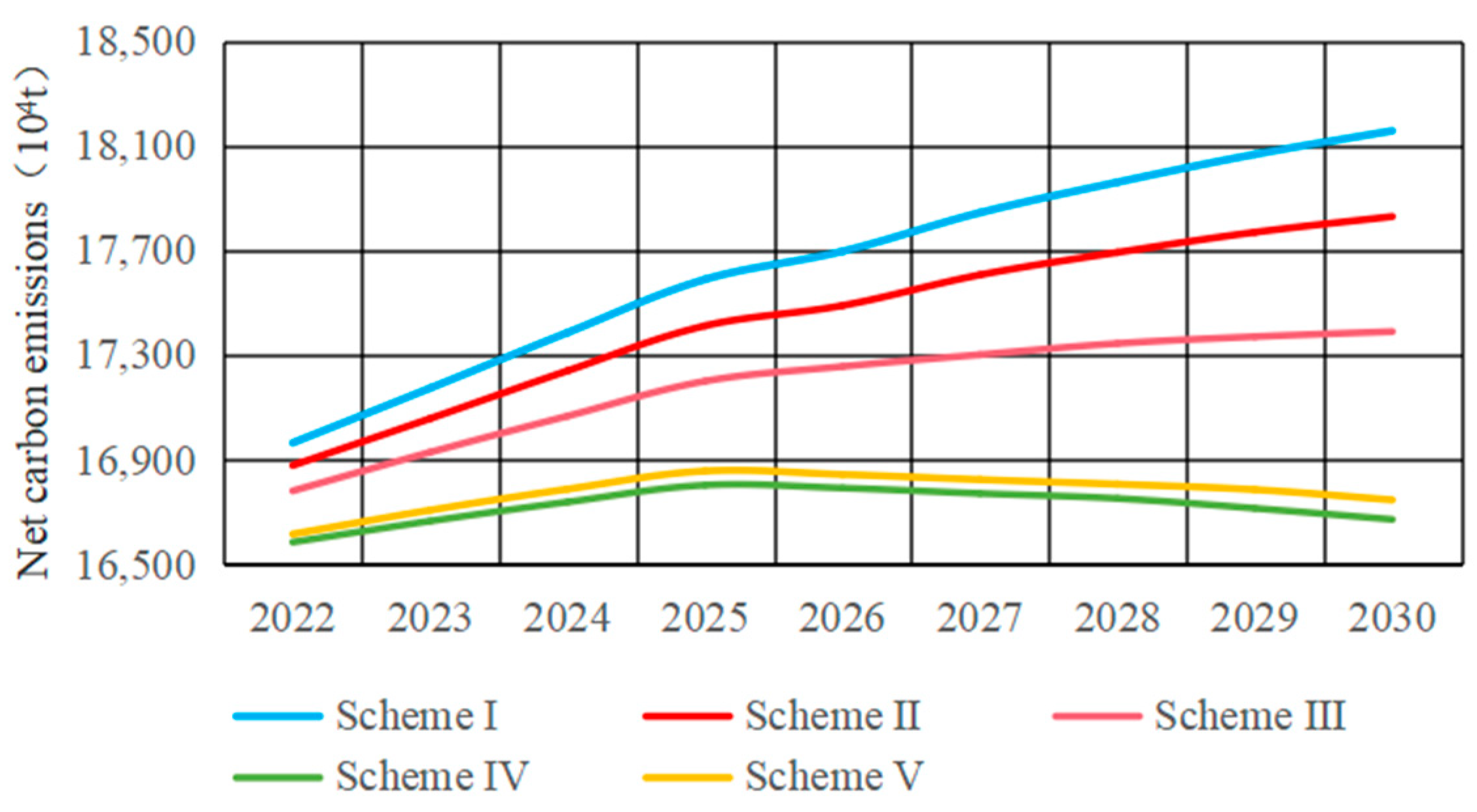
3.1. Design of Regulation Scheme for Carbon Reduction Goal

The spatial boundary of the SD model was the administrative region of Tianjin. The starting time of simulation was 2004 and the simulation time was from 2005 to 2030. The historical test period was from 2005 to 2019, and the time step was one year. We determined the model parameters according to historical data and development trend forecast. First, we used the Check Model and Units Check that comes with the Vensim software to perform the running test. The test results showed that the model structure and variable units passed the test, and the model could run normally. Additionally, we carried out the historical test by taking total population, total GDP, water demand of agriculture, water demand of manufacturing industry, domestic water demand, total water supply, arable land area, construction land area, raw coal consumption of secondary industry, household natural gas consumption, carbon sink and net carbon emissions of water and land resources utilization from 2005 to 2019 as the test variables. The simulated values of the model were compared with the actual values, and the error rate of each variable was calculated. The results showed that all the error rates were less than 10%, which are acceptable [49]. In addition, we selected twenty parameters shown in Figure 4 for model sensitivity analysis. Each parameter was increased by 15% of the original value to calculate the corresponding change range of each output variable of the system. As shown in Figure 4, the sensitivity of all the parameters was less than 15%, indicating that the model had good stability. The secondary industry GDP per unit construction land area and the tertiary industry GDP per unit construction land area were more sensitive than the other parameters. The other parameters with higher sensitivity included the net population growth rate, irrigation water quota, change in per capita residential and industrial land area, water demand per unit industry GDP, change in forest land area and the domestic water demand coefficient for urban residents. The above test results show that the SD model can be used for carbon emission simulation and prediction of water and land resources utilization in Tianjin.
Tianjin’s 13th Five Year Plan for Climate Change Mitigation put forward the goal to achieve a peak in carbon emissions around 2025, five years ahead of the 2030 promised by the state to the world. It is difficult to achieve this by taking a single measure. In real policy practice, it is also necessary to combine various emission reduction measures and adopt a comprehensive regulation scheme in order to reach the established goal of peaking carbon emissions while maintaining steady economic growth. To this end, we selected variables from each subsystem of the SD model and combined them to set up five comprehensive regulation schemes (Table 2). The increase or decrease of variables in the energy structure optimization and land use structure optimization schemes give the change in 2030 compared with the forecast results of the original model, and the increase or decrease of variables in the other regulation measures give the change in 2030 compared with the current value in 2019.
The model parameters were modified in turn according to the five schemes, and after running the model, the simulation results of the annual net carbon emissions of water and land resource utilization predicted by each scheme are shown in Figure 5. It can be seen that the carbon emissions of each scheme are sorted in descending order: scheme I > scheme II > scheme III > scheme V > scheme IV. Observing the variable settings of schemes, because the emission reduction efforts of scheme I, scheme II and scheme III are lower than those of the other two schemes, the net carbon emissions of water and land resources utilization are significantly higher than those of the other two schemes, and the net carbon emissions will continue to grow and will not reach the peak in 2030.
Tianjin is a typical resource-based water-scarce city, where the water supply is partly dependent on transfer water from other provinces. Thus, water saving is particularly important for Tianjin. Meanwhile, economic development is also the premise to ensure the sustainable development of the city. Therefore, we chose the total water demand and total GDP of scheme IV and scheme V for further analysis. The results are shown in Figure 6. It can be seen that the total water demand of scheme V is less than that of scheme IV, indicating that scheme V has higher water utilization efficiency and performs better than scheme IV in water resource utilization. The total GDP of the scheme V is larger than that of scheme IV, and has the faster economic development speed. The main reason is that the conversion of construction land into farmland in scheme V is less than that in scheme IV, and construction land can generate more GDP than farmland. Since Tianjin needs to ensure economic growth while achieving the carbon emission reduction target, Scheme V also performs better than Scheme IV considering urban economic development. Generally, the overall performance of Scheme V is better than Scheme IV.

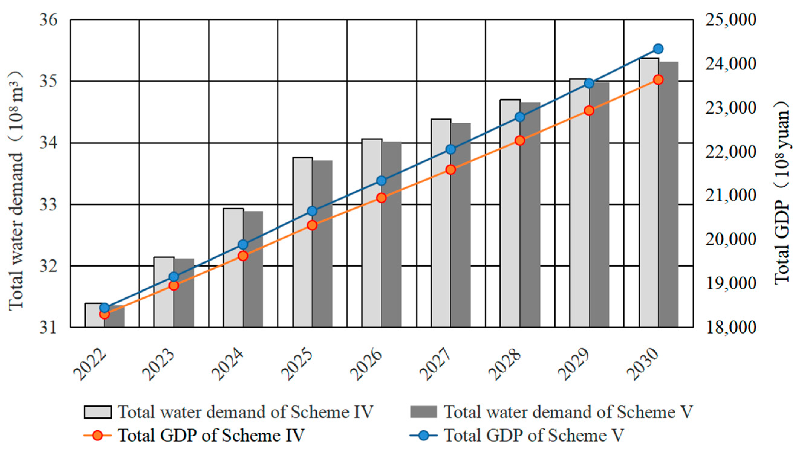
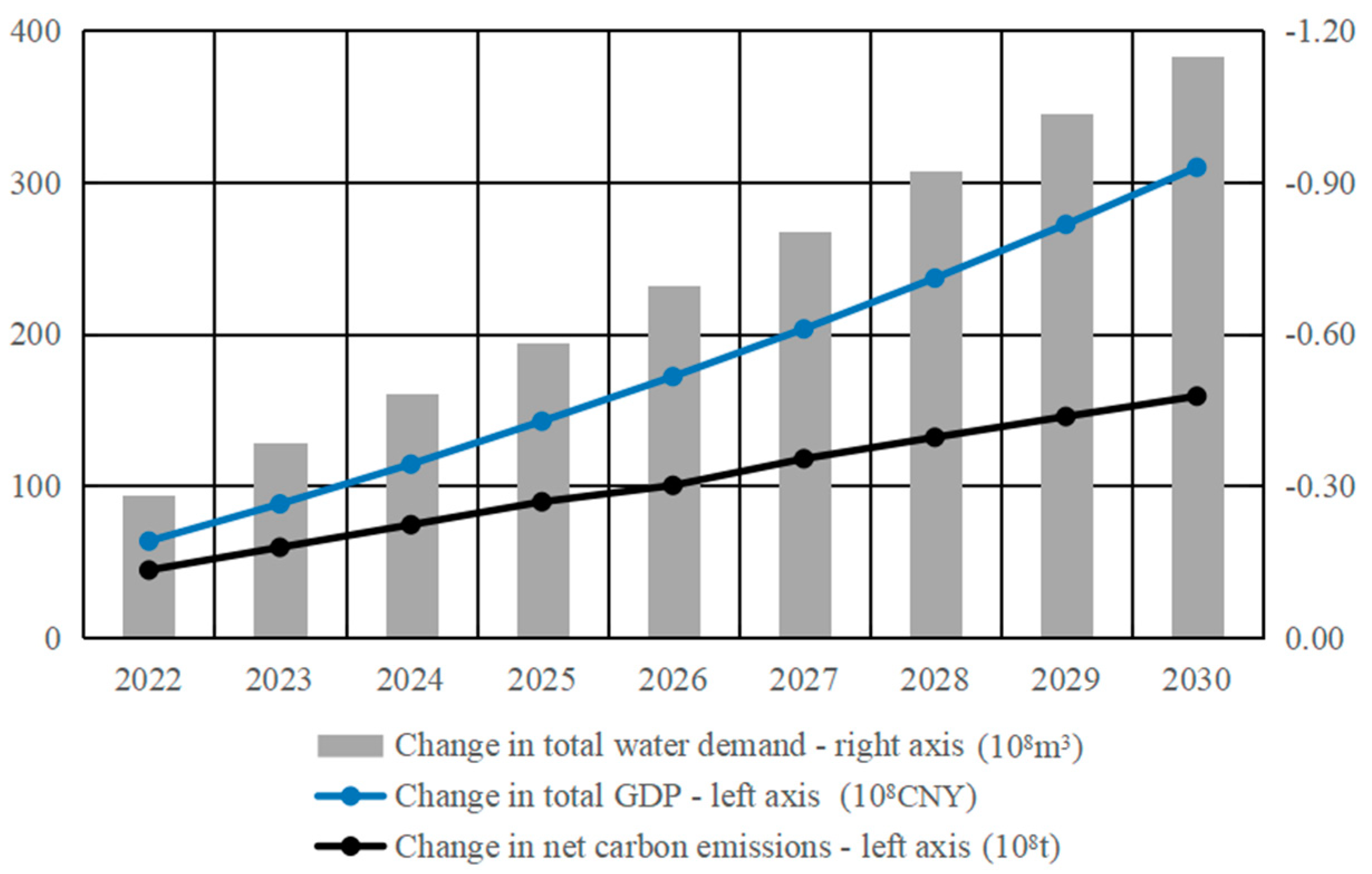
3.2. Optimization of Regulation Scheme for Low Carbon Development Goal

Urban low carbon development means coordinated promotion of economy, society and environment, which is a typical multi-objective problem. The key decision variables selected in this paper are: change in irrigation water quota ( x 1 ), change in water demand per unit industry GDP ( x 2 ), change in domestic water demand coefficient for urban residents ( x 3 ), change in per capita arable land area ( x 4 ), change in garden area ( x 5 ), change in forest land area ( x 6 ), and change in other farmland area ( x 7 ), changes in per capita residential and industrial land area ( x 8 ), and change in per capita traffic land area ( x 9 ). According to the urban water supply planning, drainage planning, land use planning, combined with the prediction of the SD model, the specific values of independent variable constraints were determined.
We wrote the NSGA-II program using Matlab software (version R2020a). The relevant parameters set were as follows: the population size was 200, the number of iterations was 500, the crossover and mutation rates were 1 and 0.11, the number of model objective functions was 3, and the number of independent variables was 9. The economic benefit objective function took a negative value, so that the optimization directions of the three objective functions were consistent, all of which were minimized. After 500 generations of evolution, individuals were distributed evenly on the Pareto front shown in Figure 7, which shows that NSGA-II has advantages in maintaining population diversity.
We assumed the TOPSIS–AHP method to seek the optimal scheme from the Pareto-optimal solutions following the four steps. Firstly, constructing the normalized initial matrix with the three objective functions including total urban water demand, total GDP and net carbon emissions of water and land resources utilization. Then, since the objective function takes minimization as the optimization objective, the minimum value of each column was selected as the positive ideal solution and the maximum value of each column was selected as the negative ideal solution. Thirdly, seven experts from universities and research institutions were invited to score the relative importance of the three objectives at a meeting in May 2021 and the judgment matrix was constructed. Among the experts, three are in the field of environmental science, two are in the field of management science and the other two are in the field of resource planning. The weight matrix of the three objective functions is W = ( 0.1226 , 0.3202 , 0.5571 ) T and CR = 0.0009 < 0.1, which passes the consistency test. Finally, we calculated the distances between the Pareto-optimal solutions and the optimal scheme, and sorted the distances. The maximum value of C i is 0.61, and the optimal solution is: x 1 = 3.13 × 10 5 , x 2 = 5.96 × 10 6 , x 3 = 3.81 × 10 5 , x 4 = 7.03 × 10 3 , x 5 = 6.12 , x 6 = 34.3 , x 7 = 15.06 , x 8 = 3.05 , x 9 = 1.88 .

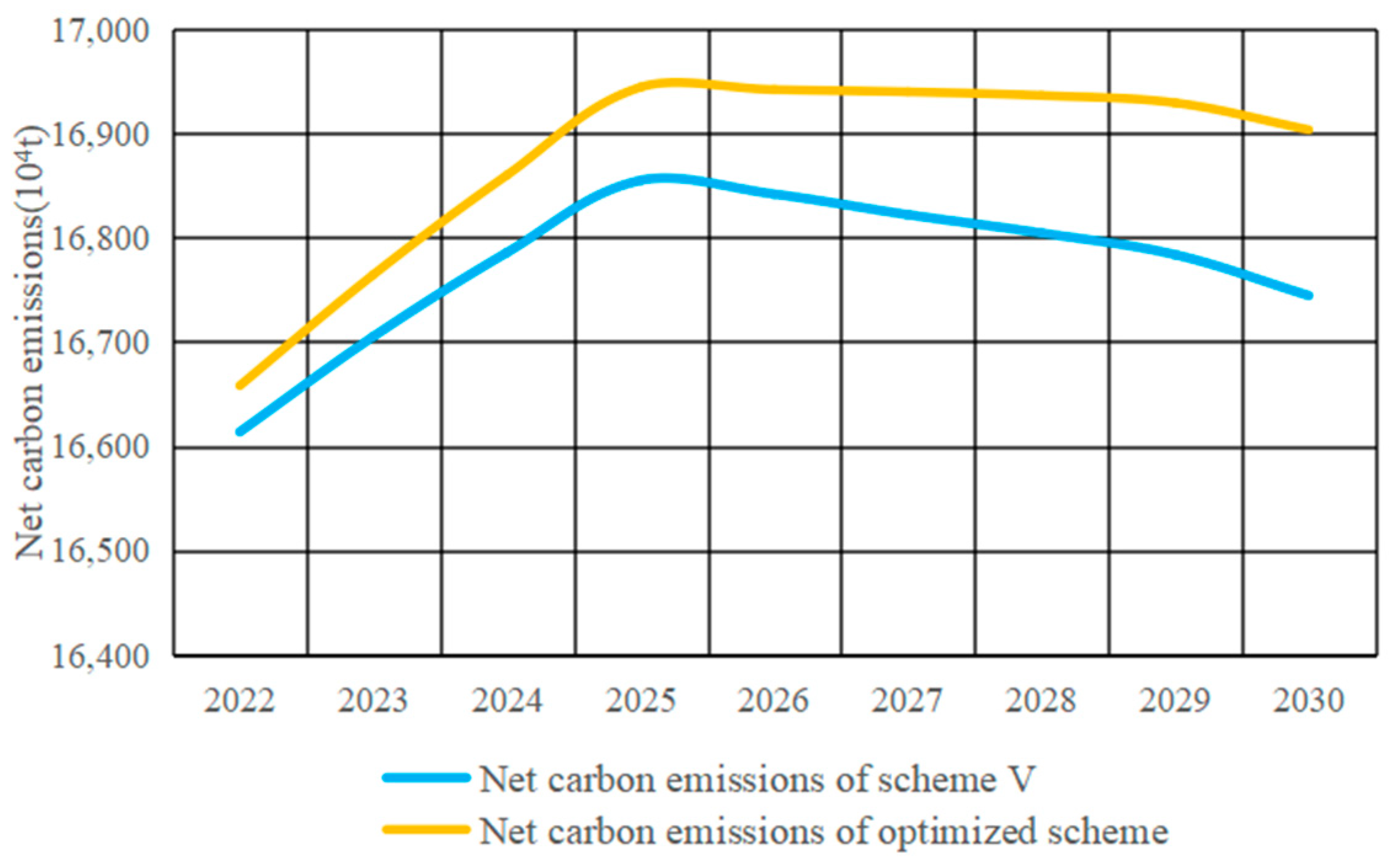
3.3. Analysis of Optimal Regulation Scheme

We substituted the optimal parameters into the SD model to compare the changes in the operating results of scheme V.
Initially, we subtracted the total water demand, total GDP and net carbon emissions of the original scheme V during the prediction period from the values of the optimized scheme to compare the changes of the objective function value, as shown in Figure 8. The results show that the total water demand of the optimized scheme was slightly lower than that of the original scheme V. It would decrease by 0.28 × 10⁴ m3 in 2022 and 1.15 × 10⁴ m3 in 2030. The total GDP of the optimized scheme was higher than that of the original scheme V. It would increase by CNY 63.4 × 10⁸ in 2022 and CNY 309.7 × 10⁸ in 2030. The net carbon emissions of the optimized scheme were also higher than that of the original scheme V. They would increase by 44.3 × 10⁴ t in 2022 and 158.9 × 10⁴ t in 2030. Since the growth rate of net carbon emissions was lower than that of total GDP, the annual carbon emissions per unit GDP during the forecast period of the optimized scheme was lower than that of the original scheme V. As shown in Figure 9, the optimized scheme would achieve the carbon peak target in 2025, which would meet the carbon emission reduction target of Tianjin. Since the GDP of the optimized scheme was higher than the original scheme, it would create greater economic development space in the future for the city in the context of COVID-19’s negative impact on society and economy.
Additionally, we analyzed the water and land resources allocation of the optimized scheme, and compared the changes between each land use type and water use of each section. The values of arable land area, garden land area, forest land area, other farmland area, residential and industrial land area, traffic land area, agricultural water demand, water demand of manufacturing industry and domestic water demand in the original scheme V during the prediction period were subtracted from the values of the optimized scheme, and they are shown in Figure 10. The results show that in terms of farmland, the arable land area, garden land area and forest land area of the optimized scheme were larger than those of the original scheme V, with an increase of 54.67 km2, 32.78 km2 and 51.7 km2, respectively in 2030. The optimized scheme has more sufficient arable land resource, which is more conducive to maintaining food security. As the main carbon sink land, garden land and forest land have a larger area after optimization, which is more conducive to absorbing carbon emissions. In addition, the increase of the area of the two land types is advantageous to improving the urban ecological environment, forest coverage and citizens’ living environment. As an important carbon source land, the area of other farmland in the optimization scheme is less than that in the original scheme V, with a reduction of 177.84 km2 in 2030, which helps to reduce carbon emissions. In terms of construction land, the area of residential and industrial land area and traffic land in the optimized scheme are higher than those in the original scheme V, with an increase of 33 km2 and 19.63 km2 in 2030, giving more space for the development of urban industry and transportation. After optimization, the area of construction land in 2030 will be basically the same as the current area, which is in line with the goal of not increasing the construction land area after 2020 proposed in Tianjin’s land use planning. In terms of water demand, the agricultural water demand, manufacturing water demand, and domestic water demand of the optimized scheme are smaller than those of the original scheme V, which will be reduced by 0.43 × 10⁸ m3, 0.23 × 10⁸ m3, and 56 × 108 m3, respectively in 2030, indicating more economical and efficient water use mode.
To sum up, although the optimized scheme produced more carbon emissions than the original scheme V, it could still reach the carbon peak goal of Tianjin. Additionally, the total economic volume of the optimized scheme was larger, which would give the urban economy more room for growth in the future. The optimized scheme would have better performance in water use efficiency, which has great significance for Tianjin, a typical resource-based water-scarce city. The allocation of urban land resource would be more reasonable, as it not only protects arable land resource, develops forest land resource that ensure food security and improve the urban ecological environment, but also strictly controls the expansion of construction land and keeps the dynamic balance of construction land by meeting the construction land objective determined in the city’s land use development plan and reserving more space for future urban development. Thus, the optimized scheme can be used as a reference decision scheme for Tianjin.

4. Conclusions and Policy Implications

4.1. Conclusions

We assumed the SD-MOP model to study the carbon emissions of urban water and land resources, which can provide a decision-making scheme for urban low carbon development. We began by describing the regulation mechanism of urban water and land resources utilization for low carbon development consisting of three elements: water resource utilization, land use, and energy development and utilization. The three elements are interrelated and are mutual resources through their water–land, land–energy, and water–energy relationships, jointly supporting human socioeconomic activities, and taking carbon emissions as the environmental effect. The coupling interactions are influenced by external factors such as socioeconomic development, resource endowment, technical progress, government regulation and social environment, and are in the process of dynamic evolution. Additionally, we established a SD model of carbon emissions for urban water and land resources utilization, and designed five regulation schemes for Tianjin. The simulation results show that two of the schemes would achieve the carbon peak in 2025, scheme V was the better option in terms of its higher total GDP and less total water demand. In closing, we identified the key variables of the SD model, and built a MOP model considering society, economy and environment benefits to further optimize the allocation parameters of water and land resources in scheme V according to the requirements of urban planning. Then, the optimized parameters obtained by the NSGA-II algorithm and TOPSIS-AHP method were input into the SD model, and the simulation results show that after optimization, Tianjin would still achieve the urban carbon peak in 2025. The urban economic level would be further improved, and the allocation of water and land resources would be more reasonable after optimization.

4.2. Policy Implications

The coupling interaction of urban water and land resources utilization and energy consumption produces carbon emissions, which are affected by socioeconomic, technology and resource endowment. Accordingly, the carbon emissions of water and land resources utilization need to be regulated by comprehensive rather than a single measure from the aspects of industrial structure, energy structure, energy efficiency, water utilization, land use structure and residents’ low carbon awareness to achieve the emission reduction target.
At present, the proportion of industrial structures in Tianjin is 1.5:34.1:64.4, while the proportion of tertiary industry in developed countries is higher than 70%. In contrast, Tianjin’s secondary industry accounts for a large proportion, while the development of tertiary industry lags far behind. The tertiary industry has greater economic contribution and comsumes less energy, thus it is necessary to further adjust the industrial structure and vigorously develop the tertiary industry to reduce carbon emissions while promoting economic growth.
With the implementation of Tianjin’s “coal-to-electricity” and “coal-to-gas” plans, Tianjin’s raw coal consumption has been greatly reduced. In the future, the energy structure adjustment to reduce coal and increase natural gas has limited potential for carbon emission reduction. The proportion of other clean energy, such as wind energy, solar energy and bioenergy, etc., should to be increased, and the energy efficiency should be improved through technological innovation, so as to promote carbon emission reduction from the energy consumption side.
Improving water use efficiency and strengthening industrial and domestic water conservation are of great significance to Tianjin, a typical water-scarce city in China. It is necessary to implement water-saving technology and strengthen water-saving publicity to reduce urban water demand, thereby reducing the carbon emissions of water resource utilization. Construction land is the main carbon source, and forest land and garden land are carbon sinks. Thus the allocation of land resources should be further optimized, which not only reserves construction land for urban development, but also strictly controls its scale by making room for carbon sink land, and enhances the land use of intensity level of construction. The forest land should be protected and developed to increase carbon sink, thereby reducing land use carbon emissions. Meanwhile, the protection and low carbon utilization of arable land should be strengthened to ensure urban food security.
Residents’ carbon emissions from daily living are an important contributor to carbon emissions of urban water and land resources utilization. It is important to improve residents’ low carbon awareness through various measures to enable them to practice low carbon lifestyles and achieve carbon emission reduction. For example, restricting the excessive packaging of commodities and the use of disposable products, encouraging green travel methods such as walking, shared bicycles, and public transportation, and inspiring the conservation and utilization of energy for daily living, such as electricity and gas saving.
Our study still has some limitations and provides opportunities for future study. First, the carbon emission accounting in this paper is based on statistical data. With the rise of the internet of things and big data, it is possible to combine the real-time monitoring data with statistical data to calculate the carbon emissions. In addition, in terms of the limitations of statistical data, some factors are simplified in the SD model. In future research, the model variables and equations can be improved in combination with the utilization characteristics of water and land resources in different cities, so as to make them more consistent with particular cities. Finally, this paper constructs an MOP model including economic, social and environmental benefits. Other optimization objectives could be added according to different research needs, such as maximizing the urban ecosystem services or maximizing water use satisfaction, etc., in future research to meet the different needs of decision makers.

Author Contributions

Conceptualization, W.J. and Z.Z. (Zhenxiang Zeng); methodology, W.J. and Z.Z. (Zhenxiang Zeng); software, W.J.; validation, Z.Z. (Zhengyun Zhang); formal analysis, W.J. and Z.Z. (Zhengyun Zhang); investigation, Y.Z.; resources, Y.Z.; data curation, Y.Z.; writing—original draft preparation, W.J.; writing—review and editing, Z.Z. (Zhenxiang Zeng); visualization, W.J.; supervision, Z.Z. (Zhengyun Zhang); project administration, Z.Z. (Zhengyun Zhang); funding acquisition, Y.Z. All authors have read and agreed to the published version of the manuscript.

Funding

This research was funded by the National Water Pollution Control and Treatment Science and Technology Major Project (2017ZX07107-001).

Institutional Review Board Statement

Not applicable.

Informed Consent Statement

Not applicable.

Data Availability Statement

The data presented in this study are available on request from the corresponding author.

Conflicts of Interest

The authors declare no conflict of interest.

References

  1. Bai, Y.; Deng, X.; Gibson, J.; Zhao, Z.; Xu, H. How does urbanization affect residential CO2 emissions? An analysis on urban agglomerations of China. J. Clean. Prod. 2019, 209, 876–885. [Google Scholar] [CrossRef]
  2. Friedlingstein, P.; O’Sullivan, M.; Jones, M.W.; Andrew, R.M.; Hauck, J.; Olsen, A.; Peters, G.P.; Peters, W.; Pongratz, J.; Sitch, S.; et al. Global carbon budget 2020. Earth Syst. Sci. Data 2020, 12, 3269–3340. [Google Scholar] [CrossRef]
  3. Mallapaty, S. How China could be carbon neutral by mid-century. Nature 2020, 586, 482–483. [Google Scholar] [CrossRef]
  4. Stoyanova, S.; Nyeste, K.; Georgieva, E.; Uchikov, P.; Velcheva, I.; Yancheva, V. Toxicological impact of a neonicotinoid insecticide and an organophosphorus fungicide on bighead carp (Hypophthalmichthys nobilis Richardson, 1845) gills: A comparative study. North-West. J. Zool. 2020, 16, 64–73. [Google Scholar]
  5. Yancheva, V.; Georgieva, E.; Stoyanova, S.; Velcheva, I.; Somogyi, D.; Nyeste, K.; Antal, L. A histopathological study on the Caucasian dwarf goby from an anthropogenically loaded site in Hungary using multiple tissues analyses. Acta Zool. 2020, 101, 431–446. [Google Scholar] [CrossRef]
  6. Skaggs, R.; Hibbard, K.A.; Frumhoff, P.C.; Lowry, T.; Middleton, R.; Pate, R.; Tidwell, V.C.; Arnold, J.G.; Averyt, K.; Janetos, A.C.; et al. Climate and Energy-Water-Land System Interactions Technical Report to the U.S. Department of Energy in Support of the National Climate Assessment; Pacific Northwest National Lab. (PNNL): Richland, WA, USA, 2012. [Google Scholar] [CrossRef] [Green Version]
  7. Zhao, R.Q.; Liu, Y.; Tian, M.M.; Ding, M.L.; Cao, L.H.; Zhang, Z.P.; Chuai, X.W.; Xiao, L.G.; Yao, L.G. Impacts of water and land resources exploitation on agricultural carbon emissions: The water-land- energy- carbon nexus. Land Use Pol. 2018, 72, 480–492. [Google Scholar] [CrossRef]
  8. Kothavala, Z.; Arain, M.A.; Black, T.A. The simulation of energy, water vapor and carbon dioxide fluxes over common crops by the Canadian Land Surface Scheme (CLASS). Agric. For. Meteorol. 2005, 133, 89–108. [Google Scholar] [CrossRef]
  9. Zhang, Y.C.; Shen, Y.J.; Xu, X.L.; Sun, H.Y.; Li, F.; Wang, Q. Characteristics of the water-energy-carbon fluxes of irrigated pear (Pyrus bretschneideri Rehd) orchards in the North China Plain. Agric. Water Manag. 2013, 128, 140–148. [Google Scholar] [CrossRef]
  10. Chhipi-Shrestha, G.; Hewage, K.; Sadiq, R. Water-energy-carbon nexus modeling for urban water systems: System dynamics approach. J. Water Resour. Plan. Manage.-ASCE 2017, 143, 04017016. [Google Scholar] [CrossRef]
  11. Wang, X.C.; Klemes, J.J.; Wang, Y.T.; Dong, X.B.; Wei, H.J.; Xu, Z.H.; Varbanov, P.S. Water-energy-carbon emissions nexus analysis of China: An environmental input-output model-based approach. Appl. Energy 2020, 261, 114431. [Google Scholar] [CrossRef]
  12. Rodriguez, N.; Armenteras, D.; Retana, J. National ecosystems services priorities for planning carbon and water resource management in Colombia. Land Use Pol. 2015, 42, 609–618. [Google Scholar] [CrossRef]
  13. Wang, J.; Epstein, H.E.; Wang, L.X. Soil CO2 flux and its controls during secondary succession. J. Geophys. Res.-Biogeosci. 2010, 115, G02005. [Google Scholar] [CrossRef]
  14. Fang, J.Y.; Chen, A.P.; Peng, C.H.; Zhao, S.Q.; Ci, L.J. Changes in forest biomass carbon storage in China between 1949 and 1998. Science 2001, 292, 2320–2322. [Google Scholar] [CrossRef] [PubMed]
  15. Ali, G.; Nitivattananon, V. Exercising multidisciplinary approach to assess interrelationship between energy use, carbon emission and land use change in a metropolitan city of Pakistan. Renew. Sust. Energ. Rev. 2012, 16, 775–786. [Google Scholar] [CrossRef]
  16. Zhang, R.S.; Matsushima, K.; Kobayashi, K. Can land use planning help mitigate transport-related carbon emissions? A case of Changzhou. Land Use Pol. 2018, 74, 32–40. [Google Scholar] [CrossRef]
  17. Chuai, X.W.; Huang, X.J.; Wang, W.J.; Zhao, R.Q.; Zhang, M.; Wu, C.Y. Land use, total carbon emissions change and low carbon land management in coastal Jiangsu, China. J. Clean. Prod. 2015, 103, 77–86. [Google Scholar] [CrossRef]
  18. Fang, K.; Heijungs, R.; Snoo, G.R.D. Theoretical exploration for the combination of the ecological, energy, carbon, and water footprints: Overview of a footprint family. Ecol. Indic. 2014, 36, 508–518. [Google Scholar] [CrossRef]
  19. Ali, Y. Carbon, water and land use accounting: Consumption vs production perspectives. Renew. Sust. Energ. Rev. 2017, 67, 921–934. [Google Scholar] [CrossRef]
  20. Watanabe, M.D.B.; Ortega, E. Dynamic emergy accounting of water and carbon ecosystem services: A model to simulate the impacts of land-use change. Ecol. Model. 2014, 271, 113–131. [Google Scholar] [CrossRef]
  21. Ballestero, E.; Alarcòn, S.; García-Bernabeu, A. Establishing politically feasible water markets: A multi-criteria approach. J. Environ. Manage. 2002, 65, 411–429. [Google Scholar] [CrossRef]
  22. Liu, D.; Ji, X.; Tang, J. A fuzzy cooperative game theoretic approach for multinational water resource spatiotemporal allocation. Eur. J. Oper. Res. 2020, 282, 1025–1037. [Google Scholar] [CrossRef]
  23. Murali, K.; Lim, M.K.; Petruzzi, N.C. Municipal groundwater management: Optimal allocation and control of a renewable natural resource. Prod. Oper. Manag. 2015, 24, 1453–1472. [Google Scholar] [CrossRef]
  24. Pennington, D.N.; Dalzell, B.; Nelson, E.; Mulla, D.; Taff, S.; Hawthorne, P.; Polasky, S. Cost-effective land use planning: Optimizing land use and land management patterns to maximize social benefits. Ecol. Econ. 2017, 139, 75–90. [Google Scholar] [CrossRef]
  25. Leibowicz, B.D. Urban land use and transportation planning for climate change mitigation: A theoretical framework. Eur. J. Oper. Res. 2020, 284, 604–616. [Google Scholar] [CrossRef]
  26. Biswas, A.; Pal, B.B. Application of fuzzy goal programming technique to land use planning in agricultural system. Omega 2005, 33, 391–398. [Google Scholar] [CrossRef]
  27. Peralta, R.C.; Cantiller, R.R.A.; Terry, J.E. Optimal large-scale conjunctive water-use planning: Case Study. J. Water Resour. Plan. Manage.-ASCE. 1995, 121, 471–478. [Google Scholar] [CrossRef]
  28. Cheng, K.; Fu, Q.; Li, T.X.; Jiang, Q.X. Regional food security risk assessment under the coordinated development of water resources. Nat. Hazards. 2015, 78, 603–619. [Google Scholar] [CrossRef]
  29. Xu, H.; Brown, D.G.; Moore, M.R.; Currie, W.S. Optimizing spatial land management to balance water quality and economic returns in a Lake Erie Watershed. Ecol. Econ. 2018, 145, 104–114. [Google Scholar] [CrossRef]
  30. Hirsch, C.; Krisztin, T.; See, L. Water resources as determinants for foreign direct investments inland-A gravity analysis of foreign land acquisitions. Ecol. Econ. 2020, 170, 106516. [Google Scholar] [CrossRef]
  31. Das, B.; Singh, A.; Panda, S.N.; Yasuda, H. Optimal land and water resources allocation policies for sustainable irrigated agriculture. Land Use Pol. 2015, 42, 527–537. [Google Scholar] [CrossRef]
  32. Chen, J.F.; Yu, C.; Cai, M.; Wang, H.; Zhou, P. Multi-objective optimal allocation of urban water resources while considering conflict resolution based on the PSO algorithm: A case study of Kunming, China. Sustainability 2020, 12, 1337. [Google Scholar] [CrossRef] [Green Version]
  33. Sepaskhah, A.R.; Azizian, A.; Tavakoli, A.R. Optimal applied water and nitrogen for winter wheat under variable seasonal rainfall and planning scenarios for consequent crops in semi-arid region. Agric. Water Manag. 2006, 84, 113–122. [Google Scholar] [CrossRef]
  34. Schwaab, J.; Deb, K.; Goodman, E.; Lautenbach, S.; Strien, M.J.V.; Grêt-Regamey, A. Improving the performance of genetic algorithms for land-use allocation problems. Int. J. Geogr. Inf. Sci. 2018, 32, 907–930. [Google Scholar] [CrossRef]
  35. Tian, J.; Guo, S.L.; Liu, D.D.; Pan, Z.K.; Hong, X.J. A fair approach for multi-objective water resources allocation. Water Resour. Manag. 2019, 33, 3633–3653. [Google Scholar] [CrossRef]
  36. West, T.A.P.; Grogan, K.A.; Swisher, M.E.; Caviglia-Harris, J.L.; Sills, E.; Harris, D.; Roberts, D.; Putz, F.E. A hybrid optimization-agent-based model of REDD plus payments to households on an old deforestation frontier in the Brazilian Amazon. Environ. Modell. Softw. 2018, 100, 159–174. [Google Scholar] [CrossRef]
  37. Lahiji, R.N.; Dinan, N.M.; Liaghati, H.; Ghaffarzadeh, H.; Vafaeinejad, A. Scenario-based estimation of catchment carbon storage: Linking multi-objective land allocation with InVEST model in a mixed agriculture-forest landscape. Front. Earth Sci. 2020, 14, 637–646. [Google Scholar] [CrossRef]
  38. Esteves, E.M.M.; Brigagao, G.V.; Morgado, C.R.V. Multi-objective optimization of integrated crop-livestock system for biofuels production: A life-cycle approach. Renew. Sust. Energ. Rev. 2021, 152, 111671. [Google Scholar] [CrossRef]
  39. Mirchi, A.; Madani, K.; Watkins, D.; Ahmad, S. Synthesis of system dynamics tools for holistic conceptualization of water resources problems. Water Resour. Manag. 2012, 26, 2421–2442. [Google Scholar] [CrossRef]
  40. Ramezanian, R.; Hajipour, M. Integrated framework of system dynamics and meta-heuristic for multi-objective land use planning problem. Landsc. Ecol. Eng. 2020, 16, 113–133. [Google Scholar] [CrossRef]
  41. Wang, Y.Z.; Alexander, F.; Ping, G. A model integrating the system dynamic model with the risk based two-stage stochastic robust programming model for agricultural-ecological water resources management. Stoch. Environ. Res. Risk Assess. 2021, 35, 1953–1968. [Google Scholar] [CrossRef]
  42. Zhang, X.H.; Zhang, H.W.; Zhang, B.A.; Liu, H.B. SD-MOP integrate model and its application in water resources plan: A case study of Qinhuangdao. Kybernetes 2010, 39, 1384–1391. [Google Scholar] [CrossRef]
  43. Xu, J.P.; Yang, J.; Yao, L.M. Transportation structure analysis using SD-MOP in World Modern Garden City: A case study in China. Discrete Dyn. Nat. Soc. 2012, 2012, 710854. [Google Scholar] [CrossRef]
  44. Deb, K.; Pratap, A.; Agarwal, S.; Meyarivan, T. A fast and elitist multi-objective genetic algorithm: NSGA-II. IEEE Trans. Evol. Comput. 2002, 6, 182–197. [Google Scholar] [CrossRef] [Green Version]
  45. Sofia, A.S.; GaneshKumar, P. Multi-objective task scheduling to minimize energy consumption and makespan of cloud computing using NSGA-II. J. Netw. Syst. Manag. 2018, 26, 463–485. [Google Scholar] [CrossRef]
  46. Azari, A.; Hamzeh, S.; Naderi, S. Multi-objective optimization of the reservoir system operation by using the hedging policy. Water Resour. Manag. 2018, 32, 2061–2078. [Google Scholar] [CrossRef]
  47. Azizi, E.; Javanshir, H.; Jafari, F.; Ebrahimnejad, S. Designing a sustainable agile retail supply chain using multi-objective optimization methods (Case study: SAIPA Company). Sci. Iran. 2021, 28, 2933–2947. [Google Scholar] [CrossRef] [Green Version]
  48. Saaty, T.L. Absolute and relative measurement with the AHP.The most livable cities in the United States. Socio-Econ. Plann. Sci. 1986, 20, 327–331. [Google Scholar] [CrossRef]
  49. Arslan, M.O.; Altinok, H. A system dynamics model of income distribution between labor and capital for turkey. Econ. Comput. Econ. Cybern. Stud. 2018, 52, 241–256. [Google Scholar] [CrossRef]
Figure 1. The conceptual model of urban water and land resources utilization and regulation mechanisms for low carbon development.
Sustainability 14 02760 g001
Figure 2. Modeling steps of the SD-MOP model. SD represents the system dynamics; MOP represents the multi-objective programming.
Sustainability 14 02760 g002
Figure 3. The causal loop diagram of the system. POP represents the population; NPGR represents the net population growth rate; UPOP represents the urban population; RPOP represents the rural population; UR represents the urbanization rate; IWD represents the irrigation water demand; WDA represents the water demand of agriculture; DWD represents the domestic water demand; UDWD represents the urban domestic water demand; RDWD represents the rural domestic water demand; ADWS represents the awareness of domestic water saving; WDGL represents the water demand of garden land; WDTI represents the water demand of tertiary industry; WDCI represents the water demand of construction industry; WDMI represents the water demand of manufacturing industry; WSP represents the water saving promotion; EWD represents the ecological water demand; TWD represents the total water demand; UDS represents the urban domestic sewage; STI represents the sewage of tertiary industry; RWS represents the reused water supply; SWGS represents the surface water and groundwater supply; TFWS represents the transfer water supply; DWS represents the desalination water supply; TWS represents the total water supply; DBWSD represents the difference between water supply and demand; ALA represents the arable land area; PL represents the protection level; FLA represents the forest land area; GLA represents the garden land area; FC represents the forest coverage; GA represents the grassland area; AOF represents the area of other farmland; FA represents the farmland area; RILA represents the residential and industrial land area; TLA represents the traffic land area; LUIL represents the land use intensity level; WCFLA represents the water conservancy facilities land area; CLA represents the construction land area; ULA represents the unused land area; AGDP represents the agriculture gross domestic product (GDP); AGPUFA represents the agriculture GDP per unit farmland area; SIGDP represents the secondary industry GDP; SIGPUCLA represents the secondary industry GDP per unit construction land area; CIGDP represents the construction industry GDP; MIGDP represents the manufacturing industry GDP; TIGDP represents the tertiary industry GDP; TIGPUCLA represents the tertiary industry GDP per unit construction land area; TGDP represents the total GDP; HGC represents the household gasoline consumption; HDC represents the household diesel consumption; HEC represents the household electricity consumption; HHC represents the household heat consumption; OFFCH represents the other fossil fuel consumption of household; RLCA represents the residents’ low carbon awareness; TPAM represents the total power of agricultural machinery; CFP represents the consumption of fertilizers and pesticides; ALCDL represents the agricultural low carbon development level; ECSI represents the electricity consumption of secondary industry; HCSI represents the heat consumption of secondary industry; OFFCSI represents the other fossil fuel consumption of secondary industry; DCTI represents the diesel consumption of tertiary industry; GCTI represents the gasoline consumption of tertiary industry; ECTI represents the electricity consumption of tertiary industry; HCTI represents the heat consumption of tertiary industry; OFFCTI represents the other fossil fuel consumption of tertiary industry; EE represents the energy efficiency; CEHWU represents the carbon emissions of household water utilization; CERL represents the carbon emissions of residential land; CEAL represents the carbon emissions of arable land; CEAW represents the carbon emissions of agricultural water; CEOF represents the carbon emissions of other farmland; CEWSST represents the carbon emissions of water supply and sewage treatment; CETL represents the carbon emissions of traffic land; CESTIWU represents the carbon emissions of secondary and tertiary industry water utilization; CESTIL represents the carbon emissions of secondary and tertiary industry land; CEWRU represents the carbon emissions of water resource utilization carbon emissions of water resource utilization; CELU represents the carbon emissions of land use; CS represents the carbon sink; NCEWLRU represents the net carbon emissions of water and land resources utilization.
Sustainability 14 02760 g003
Figure 4. The sensitivity analysis of SD model. 1. Secondary industry GDP per unit construction land area; 2. Tertiary industry GDP per unit construction land area; 3. Net population growth rate; 4. Irrigation water quota; 5. Change in per capita residential and industrial land area; 6. Water demand per unit industry GDP; 7. Change in forest land area; 8. Domestic water demand coefficient for urban residents; 9. Raw coal consumption per unit industry GDP; 10. Change in per capita traffic land area; 11. Electricity consumption per unit tertiary GDP; 12. Change in garden land area; 13. Heat consumption per unit industry GDP; 14. Per capita heat consumption; 15. Domestic water demand coefficient for rural residents; 16. Change in per capita arable land area; 17. Change in other farmland area; 18. Per capita gasoline consumption; 19. Agriculture industry GDP per unit farmland area; 20. Raw coal consumption per unit tertiary GDP.
Sustainability 14 02760 g004
Figure 5. The net carbon emissions of five comprehensive regulation schemes.
Sustainability 14 02760 g005
Figure 6. The net carbon emissions of five comprehensive regulation schemes.
Sustainability 14 02760 g006
Figure 7. The Pareto front.
Sustainability 14 02760 g007
Figure 8. Changes of simulation results between the optimized scheme and the original scheme V.
Sustainability 14 02760 g008
Figure 9. Comparison of net carbon emissions between the optimized scheme and the original scheme V.
Sustainability 14 02760 g009
Figure 10. Comparison of water and land resources allocation between the optimized scheme and the original scheme V.
Sustainability 14 02760 g010
Table 1. The main variables of each subsystem.
SubsystemMain Variables
Land use subsystemArable land area, forest land area, garden land area, grassland area, other farmland area, residential and industrial land area, traffic land area, water conservancy facilities land area, and unused land area.
Water resource utilization subsystemTotal water demand, water demand of agriculture, water demand of manufacturing industry, water demand of tertiary industry, water demand of construction industry, domestic water demand, ecological water demand, total water supply, surface water and groundwater supply, transfer water supply, desalination water supply, and reused water supply.
Economic subsystemTotal GDP, agriculture GDP, secondary industry GDP, tertiary industry GDP, agriculture GDP per unit farmland area, secondary industry GDP per unit construction land area, and tertiary industry GDP per unit construction land area.
Population subsystemTotal population, urban population, rural population, and net population growth rate.
Energy consumption subsystemElectricity/heat/other fossil fuel consumption of secondary industry, electricity/heat/diesel/gasoline/other fossil fuel consumption of tertiary industry and household, and total power of agricultural machinery.
Table 2. The comprehensive regulation schemes for carbon emissions of water and land resources in Tianjin.
Regulation MeasuresVariable SettingsScheme IScheme IIScheme IIIScheme IVScheme V
Industrial structure optimizationProportion of secondary industry GDP6 percentage points decrease7 percentage points decrease7 percentage points decrease8 percentage points decrease8 percentage points decrease
Proportion of tertiary industry GDP6 percentage points increase7 percentage points increase7 percentage points increase8 percentage points increase8 percentage points increase
Industrial energy efficiency improvementEnergy consumption per unit GDP of secondary industry/tertiary industry32% decrease34% decrease34% decrease35% decrease35% decrease
Increasing of residents’ low carbon awarenessPer capita residential energy consumption2% decrease2% decrease4% decrease4% decrease5% decrease
Energy structure optimizationProportion of raw coal consumption of secondary industry0.65 percentage points decrease1 percentage points decrease1 percentage points decrease1.35 percentage points decrease1.35 percentage points decrease
Proportion of natural gas consumption of secondary industry0.65 percentage points increase1 percentage points increase1 percentage points increase1.35 percentage points increase1.35 percentage points increase
Proportion of raw coal consumption of tertiary industry/household0.03 percentage points decrease0.04 percentage points decrease0.04 percentage points decrease0.05 percentage points decrease0.05 percentage points decrease
Proportion of natural gas consumption of tertiary industry/household0.03 percentage points increase0.04 percentage points increase0.04 percentage points increase0.05 percentage points increase0.05 percentage points increase
Water saving irrigationIrrigation water quota2% decrease2% decrease3% decrease3% decrease5% decrease
Industrial water savingWater demand per unit of industry GDP3% decrease3% decrease5% decrease5% decrease7% decrease
Domestic water savingDomestic water demand coefficient for urban residents1% decrease1% decrease2% decrease2% decrease3% decrease
Land use structure optimizationProportion of farmland1.5 percentage points increase2 percentage points increase2 percentage points increase3.5 percentage points increase2.5 percentage points increase
Proportion of construction land1.5 percentage points decrease2 percentage points decrease2 percentage points decrease3.5 percentage points decrease2.5 percentage points decrease
Publisher’s Note: MDPI stays neutral with regard to jurisdictional claims in published maps and institutional affiliations.

