What Are the Sectors Contributing to the Exceedance of European Air Quality Standards over the Iberian Peninsula? A Source Contribution Analysis

Abstract

The Iberian Peninsula, located in southwestern Europe, is exposed to frequent exceedances of different threshold and limit values of air pollution, mainly related to particulate matter, ozone, and nitrous oxide. Source apportionment modeling represents a useful modeling tool for evaluating the contribution of different emission sources or sectors and for designing useful mitigation strategies. In this sense, this work assesses the impact of various emission sectors on air pollution levels over the Iberian Peninsula using a source contribution analysis (zero-out method). The methodology includes the use of the regional WRF + CHIMERE modeling system (coupled to EMEP emissions). In order to represent the sensitivity of the chemistry and transport of gas-phase pollutants and aerosols, several emission sectors have been zeroed-out to quantify the influence of different sources in the area, such as on-road traffic or other mobile sources, combustion in energy generation, industrial emissions or agriculture, among others. The sensitivity analysis indicates that large reductions of precursor emissions (coming mainly from energy generation, road traffic, and maritime-harbor emissions) are needed for improving air quality and attaining the thresholds set in the European Directive 2008/50/EC over the Iberian Peninsula.

1. Introduction

Atmospheric pollution has become one of the most important health and environmental problems worldwide, affecting industrialized and developing countries around the world. Its importance and implications for sustainability have been recognized by the United Nations in their Sustainable Development Goals (SDGs) [1]. Health-relevant indicators of household and ambient pollution exposure and disease burden are included in the formal system of SDG indicators. Targets of particular relevance to ambient and household air pollution include SDG target 3.9.1, which calls for a substantial reduction in the number of deaths and illnesses from air pollution [2,3], or SDG target 11.6.2, which aims to reduce the environmental impact of cities by improving air quality [4,5].

The exposure of humans to air pollution (both photochemical and particulate matter) may be the source of many health problems ([6,7,8,9,10,11,12], among many others). The use of chemistry transport models (CTMs) can be a useful tool for assessing these air quality-related health problems. Recently, the premature deaths and the costs of the health impacts of air pollution in Europe were calculated by using ground-level concentrations from different CTMs, indicating that the total number of premature deaths (acute and chronic) ranges from 500,000 to 800,000; their associated costs are around EUR 300 billion [11,13,14].

The Iberian Peninsula (IP), especially, presents serious problems that are related mainly to tropospheric ozone (O${}_3$) [15], sulphur dioxide (SO${}_2$), nitrogen dioxide (NO${}_2$), and particles of different diameters: particulate matter with a diameter of less than 10 (PM${}_{10}$) and more than 2.5 $\mathsf{\mu }$m (PM${}_{2.5}$) [16]. In this sense, a number of studies have covered the entire IP using modeling techniques [17,18,19,20,21,22]. The results of these previous works indicate that achieving the objectives proposed by the EU directives are more difficult in the IP when compared northern countries, partly due to their particular emission distribution [23,24], and partly due to different meteorological situations, namely: (1) a lower precipitation rate (and, hence, a higher resuspension rate due to soil dryness); (2) the increased formation of secondary aerosols associated with the higher temperatures; (3) an enhanced frequency of African dust outbreaks; and (4) the higher occurrence of the recirculation of air masses that prevent air renovation [20,25].

Moreover, air pollution problems will become even more severe under future climates [26,27,28,29,30,31]. Therefore, reliable estimations of air pollution for present-day conditions and an enhanced understanding of the chemico-physical processes occurring in the atmosphere become essential, not only for informing and alerting the population, but also to understand the causes of those episodes and to implement effective abatement policies.

For that purpose, CTMs are essential for defining, evaluating, and implementing emission abatement plans through the use of sensitivity analysis strategies [32,33]. These strategies have, as a first step, the accurate identification of pollution sources and their individual contributions to the concentrations of atmospheric pollutants. To this end, a wide range of modeling methodologies has been proposed and applied for the apportionment of atmospheric pollutants [34,35,36,37]. Particularly, source apportionment relies on the determination of the contribution of different sources to pollutant concentrations by establishing the mass continuity relationships between emissions and concentrations at receptor locations. Sensitivity analyses measure how pollutant concentrations at receptors respond to perturbations at sources. Most of the sensitivity questions are left to modelers since the experimental approach is difficult and expensive.

The traditional approach to sensitivity consists in performing “twin simulations”, with one parameter perturbed [34]. In the case of the most straightforward method to assess sensitivity (brute-force method, BFM), the perturbed parameter is emissions. In the BFM, a model simulation is conducted and repeated with modified emissions, comparing the outputs of the simulations [38,39]. This method is limited because the computational cost depends, in a linear way, on the number of perturbations to examine and the strong influence of the numerical errors when the changes in the concentrations are small. Related to the BFM, the zero-out method [40,41] sets a specific emissioin sector to zero and measures the change produced in the output concentrations. In this sense, it can be considered as an extreme case of the BFM.

Since the management of air pollutant emissions is one of the predominant factors for abating urban air quality, this work assesses the source contribution of different emitting sectors to the air pollution levels in the IP, taking a particular look at the number of exceedances of air quality limits and thresholds related to health issues. For that, the WRF (meteorology) + CHIMERE (chemistry transport) modeling system has been used for a summer and a winter period over the IP in order to assess air quality-related problems in the area.

2. Materials and Methods

2.1. Modeling System

The modeling system applied consists in the Weather Research and Forecasting (WRF, meteorology) + CHIMERE (chemistry transport model) + EMEP (emissions) methods. The simulations cover the entire IP (excluding a blending area of five grid points), have a resolution of 9 km, and have been run and evaluated on an hourly basis during a period covering a summer and a winter scenario (months of June–July–August 2011, JJA, and December 2011–January–February 2012, DJF). Precisely, the simulation period ranges from 24 May 2011 to 1 September 2011, and from 23 November 2011 to 1 March 2012, with the first week being the spin-up period. The election of the 9-km resolution was conditioned by a compromise between the use of high resolutions and the computational time needed for the ensemble of simulations to be conducted in this analysis.

The regional modeling system consists of the Advanced Research Weather Research and Forecasting (WRF-ARW) Model v3.9.1 [42,43], which provides the meteorology to the CTM. WRF is a fully compressible, Eulerian, non-hydrostatic model that solves the equations that govern the atmospheric motions. A total of 33 vertical layers on sigma coordinates cover the region from the ground level up to 10 hPa. The boundary conditions used for driving the WRF simulations are obtained from the ERA-Interim reanalysis [44] every six hours. WRF fields have been coupled off-line on an hourly basis to CHIMERE CTM [45]. With respect to the CHIMERE configuration, the MELCHIOR2 gas-phase mechanism has been used [46].

Regarding the inclusion of particles within the CTM, CHIMERE includes aerosol and heterogeneous chemistry. Different chemical aerosol components have been included in the model configuration, namely, ammonium, nitrate, sulphate, and organic and elemental carbon with three subcomponents: (1) primary aerosol, (2) secondary anthropogenic, and (3) secondary biogenic subcomponents. Marine aerosols (sea salt) have also been included in the simulation. The aerosol microphysical description is based on a sectional aerosol approach that includes 6 bins using a geometrical progression and ranging from 10 nm to 40 $\mathsf{\mu }$m.

Table 1. Parameterizations of the meteorological and chemistry transport model used in the simulations for the IP.

WRF (Meteorological Model) [42,43]	CHIMERE (Chemistry Transport Model) [45]
Microphysics: WSM6 [47]	Chemical Mechanism: MELCHIOR2 [46]
PBL: Yonsei University [48]	Aerosol chemistry: Inorganic (thermodynamic equilibrium with ISORROPIA module) [49]
Radiation: CAM [50]	Organic aerosol chemistry: [51]
Soil: Noah LSM [52]	Natural aerosols: dust, re-suspended, and inert sea-salt [45]
Cumulus: Kain–Fritsch [53]	Emissions: anthropogenic emissions EMEP [54] + biogenic emissions MEGAN (Model of Emissions of Gases and Aerosols from Nature) [55]
Boundary conditions: ERA-Interim [44]	Boundary conditions: LMDz-INCA+GOCART [56]

summarizes the physico-chemical options for the regional modeling system.

Here, the climatological boundary conditions for the CTM are based on the LMDz-INCA global chemistry/climate model [57]. Other considerations to bear in mind, with respect to the boundary conditions, are that (1) the changes in stratospheric ozone are very limited and, hence, are neglected in the simulations, and (2) it has been assumed that long-range transport over the IP is limited and overwhelmed by local processes [58]. This assumption is hampered by the persistent outbreaks of Saharan dust over the IP, which may exert an important influence on the regional PM${}_{10}$ levels over Spain and Portugal [59,60]. However, this contribution focuses on a sensitivity analysis of antropogenic emissions, and hence, the impact of desert sources and their influence on the air quality of the IP is beyond the scope of this work.

Anthropogenic emissions are obtained from the EMEP database [54] and cover the entire period of simulations. Natural emissions have been estimated with the MEGAN model [55] and include species such as monoterpene, isoprene, and other biogenic volatile organic compounds (BVOCs). The meteorological inputs needed for the estimation of emissions are obtained from the WRF simulations previously described.

2.2. Sensitivity Analysis: The Zero-Out Method

The sensitivity analysis methods perturb inputs to the modeling system (e.g., modify the emissions of sulphur oxides) and quantify the response of the model output (e.g., change in sulphate concentration). As commented on before, there are several approaches for a sensitivity analysis based on the BFM in order to study the contribution from different sources; a zero-out method has been applied in this study because of its simplicity. Here, the methodology includes a base model, run with all emission sources (BC), and ten emission scenarios in which emissions from anthropogenic sources (classified according to the SNAP) are excluded, analogously to previous works [37,61,62].

The zero-out method has been extensively used for source attribution because it seems intuitive and obvious that the removal of an emission source should quantify the corresponding impact of that emission source [40,41,63]. Despite that this methodology is valid and widely used for sensitivity analysis (as in our case), it should be carefully considered for areas with a strong secondary production, because the sum of zero-out impacts over all sources may not be exactly equal to the total concentration when considering non-linear systems as those represented by atmospheric processes [34]. In this sense, Clappier et al. [36] warn that, when the non-linearity of the relationship between concentrations and emissions is noticeable, source apportionment methods may not be appropriate to assess the impact of mitigation or abatement strategies. When non-linearity is limited or negligible, source apportionment methods may be acceptable, bearing in mind the complexity of the models involved in the representation of air pollution.

Since our objective is to conduct a source apportionment analysis for the IP, the zero-out method has been applied to all the SNAP activities, including anthropogenic sources (

Table 2. Tags for the different simulations included in this contribution. The scenarios are run while zeroing-out the emissions specified by the SNAP sector.

SNAP	Emissions Zeroed-Out
SNAP1	Combustion in energy and transformation industries
SNAP2	Non-industrial combustion plants, including private wood combustion
SNAP3	Combustion in manufacturing industry
SNAP4	Production processes
SNAP5	Extraction and distribution of fossil fuels and geothermal energy
SNAP6	Solvents and other product use
SNAP7	Road transport
SNAP8	Other mobile sources and machinery (excl. international ship traffic)
SNAP9	Waste treatment and disposal
SNAP10	Agriculture
Base Case (BC)	No emissions zeroed-out

). The sensitivity to air pollution levels of these sources is covered and identified in the simulations (harbors and ships, industries, road transport, central heating, agriculture, etc.).

3. Results

3.1. Evaluation of the Modeling Results

Despite that the goal of this contribution is not to provide a comprehensive evaluation of the air quality concentrations simulated by WRF + CHIMERE, the results from the monitoring network EMEP have been used to characterize the skill of the model for reproducing the concentrations of air pollutants (EMEP data available online at: http://www.emep.int (accessed on 8 May 2012); see [64] for further details). The ten stations with simultaneous data of tropospheric O${}_3$, NO${}_2$, and PM${}_{10}$ in the IP (SO${}_2$ and PM${}_{2.5}$ have been excluded because of the scarcity of data for the target period) have been used for the model evaluation. Their location is shown in Figure 1.

The available EMEP measurements were filtered before comparing the model results with EMEP data in order to remove uncertain data (for instance, those data before a calibration of equipment or after an interruption was eliminated). In addition, after the EMEP data is filtered, the criteria of temporal coverage >85% were selected for measurement sites. Since EMEP stations are located far from large emission sources (more than 10 km), the data are assumed to fit the resolution of the model used for regional background concentrations ([64] and references therein).

A number of common metrics were used to examine the model skills, differencing between gas-phase and particulate matter. For gases, two scores have been selected: mean normalized gross error (MNGE)—which indicates the performance of the simulations to represent the magnitude of the observation—and the mean normalized bias error (MNBE)—another common parameter that reveals the departure between observations and modeling data. These provide a useful quantification of the overall under- or overestimations of the model.

As for the particulate matter evaluation, a number of authors (e.g., [16,65,66,67], among many others) suggested using the mean fractional bias (MFB) and the mean fractional error (MFE) instead of MNBE or MNGE (

Table 3. Statistical figures used in the evaluation of the WRF + CHIMERE modeling system. N: number of observations available. $C_{mod}$: model concentration. $C_{obs}$: observation concentration.

Value	Formula	Range
Model Mean (MM)	$\frac{1}{N}\sum C_{mod}$	0, +∞
Observations Mean (OM)	$\frac{1}{N}\sum C_{obs}$	0, +∞
Mean Normalized Bias Error (MNBE)	$\frac{1}{N}\sum \frac{\left(C_{mod}-C_{obs}\right)}{C_{obs}}$	−∞, +∞
Mean Normalized Gross Error (MNGE)	$\frac{1}{N}\sum \frac{\left|C_{mod}-C_{obs}\right|}{C_{obs}}$	0,+∞
Mean Fractional Bias (MFB)	$\frac{1}{N}\sum \left(\frac{(C_{mod}-C_{obs})}{\left(\frac{C_{mod}+C_{obs}}{2}\right)}\right)$	−200, +200
Mean Fractional Error (MFE)	$\frac{1}{N}\sum \left(\frac{|C_{mod}-C_{obs}|}{\left(\frac{C_{mod}+C_{obs}}{2}\right)}\right)$	0, +200

). Boylan and Russell [65] propose that a model performance goal is met when both the MFE and MBE are less than or equal to 50% and ±30%, respectively, and a model performance criterion is met when the MFE ≤75% and MFB is less than or equal to ±60%.

Therefore, MNBE and MNGE have been used for gaseous pollutants, while for particulate matter, the MFB and MFE have been utilized. A general pattern of the air pollution levels provided by WRF + CHIMERE simulations can be found in Figure 2. Maximum O${}_3$ concentrations are modeled for summertime in the easternmost part of the IP, with ground levels that exceed 120 $\mathsf{\mu }$g m${}^{-3}$ as the daily mean in Catalonia (northeastern IP). For NO${}_2$, monthly means can be as high as 50 $\mathsf{\mu }$g m${}^{-3}$ in the largest cities of the peninsula (e.g., Madrid, Lisbon, Porto) and in an industrial area such as Algeciras Bay (southernmost part of the IP), where industrial emissions are increased by port and maritime activity. The Algeciras port (the second most important port of Spain), located at the head of the bay, has a strategic importance in terms of the maritime traffic of fuel and general supplies [68]. Hence, the presence of this port makes the area of the Algeciras Bay a high risk environment for pollution derived from its commercial activities. For SO${}_2$, besides Algeciras, levels are over 20 $\mathsf{\mu }$g m${}^{-3}$ downwind of several power plants (As Pontes, in northern Spain; and Andorra (Teruel), in the eastern IP) that burn coal for the generation of electricity [69,70]. Last, particulate matter does not exhibit a clear spatial pattern in the IP. The spatial patterns depend both on the industrialization of the regions, especially regarding inorganic particulate matter, and the Saharan dust outbreaks [20]. In this sense, PM${}_{2.5}$ and PM${}_{10}$ seasonal patterns showed maximum concentrations during summertime, as is also indicated by the scientific literature.

Regarding model validation, overall, negative fractional biases are calculated for PM${}_{10}$ and NO${}_2$, while positive deviations for O${}_3$ are obtained when comparing the base-case simulation to EMEP stations (

Table 4. Model evaluation against EMEP stations. (Top) Summer (JJA) and (bottom) winter (DJF).

Summer	JJA 2011	PM${}_{10}$		NO${}_2$		O${}_3$
Code	Station Name	MFB (%)	MFE (%)	MNBE (%)	MNGE (%)	MNBE (%)	MNGE (%)
	Performance Criteria	≤±60% ${}^{\mathbf{1}}$	≤+75% ${}^{\mathbf{1}}$		≤+50% ${}^{\mathbf{2}}$		≤+50% ${}^{\mathbf{2}}$
ES07	Víznar	−38.8	68.8	−28.9	41.9	23.1	24.9
ES08	Niembro	−9.0	42.6	−19.0	41.6	22.1	22.1
ES09	Campisábalos	−54.0	54.1	−35.8	49.0	5.0	25.7
ES10	Cabo de Creus	−41.9	43.7	−15.2	33.6	1.5	26.7
ES11	Barcarrota	−58.9	68.9	−45.5	46.1	22.3	26.4
ES12	Zarra	−52.5	53.0	−46.8	49.3	20.3	24.2
ES13	Peñausende	−55.1	57.0	−28.5	59.4	11.2	12.5
ES14	Els Torms	−48.6	49.2	−34.7	44.9	20.3	21.0
ES15	Risco Llano	−52.5	62.5	−47.3	47.3	24.9	25.6
ES16	O Saviñao	6.8	41.8	18.3	40.9	32.3	33.9
Winter	DJF 2011	PM${}_{\mathbf{10}}$		NO${}_{\mathbf{2}}$		O${}_{\mathbf{3}}$
Code	Station Name	MFB (%)	MFE (%)	MNBE (%)	MNGE (%)	MNBE (%)	MNGE (%)
	Performance Criteria	≤±60% ${}^{\mathbf{1}}$	≤+75% ${}^{\mathbf{1}}$		≤+50% ${}^{\mathbf{2}}$		≤+50% ${}^{\mathbf{2}}$
ES07	Víznar	−55.7	55.8	−41.8	48.3	23.0	25.9
ES08	Niembro	−17.1	21.7	−17.1	21.7	8.3	8.3
ES09	Campisábalos	−28.7	57.2	−36.1	48.0	2.0	15.0
ES10	Cabo de Creus	−34.8	35.2	−17.8	27.7	2.2	25.5
ES11	Barcarrota	−21.6	34.9	−13.0	31.9	23.6	24.9
ES12	Zarra	−20.7	34.2	−20.7	34.2	29.8	29.8
ES13	Peñausende	−8.3	35.4	0.3	38.5	19.8	20.2
ES14	Els Torms	−34.3	45.8	−31.3	44.2	30.2	32.4
ES15	Risco Llano	−37.7	58.0	−39.6	48.9	26.0	26.6
ES16	O Saviñao	−11.3	28.2	−7.8	26.3	17.1	17.3

MFB: Mean Fractional Bias; MFE: Mean Fractional Error; MNGE: Mean Normalized Gross Error; MNBE: Mean Normalized Bias Error. ${}^1$ Boylan and Russell [65]; ${}^2$ EU Directive 2008/50/EC Uncertainty.

).

With respect to gaseous pollutants, the WRF + CHIMERE model presents a MNGE under 50% for NO${}_2$, which is the value set by the EU Directive 2008/50/EC uncertainty criteria. However, this pollutant is underestimated in both seasons and in all stations (except for in summer in ES16-O Saviñao and winter in ES13-Peñausende), possibly due to uncertainties in emission inventories [71] and the relatively coarse horizontal resolution used, which represents only partially the spatial gradient of the emissions [72]. Negative biases vary between −8% in wintertime in ES16-O Saviñao (northwestern Spain) and −47% in ES12-Zarra (at the Levantine Spanish coast). Tropospheric O${}_3$ is generally overestimated (bias under +20% in summer and under +30% during wintertime). This is related to the NO${}_2$ underestimation, limiting the titration of tropospheric O${}_3$ by NO${}_2$. Moreover, the CHIMERE lateral boundary conditions for O${}_3$ are overestimated [57,72], especially during wintertime, and therefore, the positive biases during the cold season (ranging from 2% at ES09-Campisábalos to 30% at ES14-Els Torms, northeastern Spain) are attributable to the overestimation of the background concentrations at the boundaries of the domain.

For particulate matter (PM${}_{10}$), the magnitude of the MFB and MFE are similar in both seasons, meeting the performance criteria established by Boylan and Russell [65] for all stations and during all seasons. There is a pervasive tendency to underestimate PM${}_{10}$ levels (negative MFB in all stations and both seasons, except for station ES16-O Saviñao, northwestern Spain, in summer). This summer MFB ranges from −9% in ES08-Niembro station (northern Spain) to −59% in ES11-Barcarrota (southwestern Spain). In wintertime, the maximum MFB is −56% in ES07-Víznar (southern Spain), while the minimum MFB is estimated in ES13-Peñausende (western Spain, near the Portuguese border) as −8%. More interesting is the fact that high MFEs are found in ES07-Víznar station for both seasons (68% in summer and 56% in winter). The MFB is strongly negative and almost coincident with the MFE (e.g., −56% for the MFB error in wintertime and 56% for the MFE during this season). This could be caused by the high contribution of Saharan dust at this location [25,73], which is pervasively underestimated by CTMs in southern Mediterranean stations, especially regarding the peak levels [74,75,76].

3.2. Source Contribution

Figure 3 and Figure 4 represent the results of the source contribution experiment for summertime and wintertime, respectively. The information shown in those Figures is quantified in

Table 5. Variation in the mean and maximum levels of atmospheric pollutants over the entire IP when zeroing-out the different SNAP sectors (base case minus zeroed-out SNAP sector simulation; hence, a positive value indicates an improvement in air quality).

Summer	Summer (JJA)
	Concentration	Base Case	w/o SNAP	Reduction
Pollutant	Mean ($\mathsf{\mu }$g m${}^{-3}$)	Max ($\mathsf{\mu }$g m${}^{-3}$)	Zero-out sector	Mean	Max
Tropospheric ozone, O${}_3$	132.5	164.6	SNAP7	2.3%	5.7%
			SNAP8	5.0%	1.9%
Nitrogen dioxide, NO${}_2$	66.6	124.2	SNAP8	47.4%	37.1%
Sulphur dioxide, SO${}_2$	33.0	70.7	SNAP1	2.0%	2.4%
			SNAP8	40.9%	40.3%
Particulate matter $\varphi <10\mathsf{\mu }$m, PM${}_{10}$	38.7	62.2	SNAP1	6.2%	4.3%
			SNAP8	7.0%	2.6%
			SNAP10	5.7%	2.6%
Particulate matter $\varphi <2.5\mathsf{\mu }$m, PM${}_{2.5}$	19.7	29.3	SNAP1	0.0%	4.8%
			SNAP8	0.0%	2.4%
			SNAP10	5.1%	4.8%
Winter	Winter (DJF)
	Concentration	Base Case	w/o SNAP	Reduction
Pollutant	Mean ($\mathsf{\mu }$g m${}^{-3}$)	Max ($\mathsf{\mu }$g m${}^{-3}$)	Zero-out sector	Mean	Max
Tropospheric ozone, O${}_3$	95.8	103.7	SNAP7	−1.2%	−2.3%
Nitrogen dioxide, NO${}_2$	60.0	95.4	SNAP7	32.9%	17.7%
			SNAP8	12.3%	9.7%
Sulphur dioxide, SO${}_2$	33.0	70.7	SNAP1	4.5%	3.6%
			SNAP8	2.5%	22.2%
Particulate matter $\varphi <10\mathsf{\mu }$m, PM${}_{10}$	54.3	93.5	SNAP4	6.6%	17.5%
			SNAP7	3.9%	3.3%
			SNAP10	14.0%	13.8%
Particulate matter $\varphi <2.5\mathsf{\mu }$m, PM${}_{2.5}$	21.0	34.4	SNAP1	4.7%	3.7%
			SNAP7	5.3%	4.0%
			SNAP10	16.1%	14.3%

, which indicates the relative reductions in the areas with the worst air quality in the entire IP (that is, reductions in those locations of the target domain where the daily mean and the daily mean of max. 1-hr ground-level air quality concentrations are the highest). The results are shown with respect to the base-case scenario (BC), and focus only on anthropogenic sectors (that is, excluding, for instance, the contribution of background concentrations or external transport, which cannot be controlled in abatement strategies). Overall, Table 5 indicates that the maximum reductions in air pollution levels are achieved when zeroing-out three SNAP sectors, as expected from the scientific literature: combustion in energy and transformation industries (SNAP1), road transport (SNAP7), and other mobile sources (SNAP8). The most important added value of this contribution, nonetheless, is the quantification of the respective contributions of these aforementioned sectors. For the sake of brevity, our analysis below focuses only on the assessment of the contribution from these sectors (despite that agriculture, SNAP10, may play also an important role for SO${}_2$ and particulate matter).

For tropospheric O${}_3$, on-road traffic (SNAP7) is the most important contributor in summertime. The highest daily mean levels of tropospheric O${}_3$ during summer (133 $\mathsf{\mu }$g m${}^{-3}$) reduce by 2%, while 1-hmaximum concentrations (165 $\mathsf{\mu }$g m${}^{-3}$) decrease by 6%. In addition, zeroing-out other mobile sources (SNAP8) reduces the highest daily mean and 1-h maximum O${}_3$ summertime levels by 5% and 2%, respectively. On the contrary, zeroing-out on-road traffic (SNAP7) during winter slightly contributes to an increase in tropospheric O${}_3$ concentrations (1% and 2% in wintertime, mean and maximum concentration, 96 and 104 $\mathsf{\mu }$g m${}^{-3}$, respectively), but this increase does not involve the exceedance of the objective value, as will be shown later in Section 3.4.

The response of tropospheric O${}_3$ to changes in their precursors (nitrogen oxides, NOx, and volatile organic compounds (VOCs)) has been widely covered in the scientific literature, and particularly over the IP [77,78]. Overall, under certain conditions, O${}_3$ concentrations are reduced when NOx emissions decrease. This chemical regime is denoted as NOx-sensitive conditions. Conversely, under other conditions, tropospheric O${}_3$ reduces its levels when VOC emissions (particularly, non-methane volatile organic compounds, NMVOCs) are reduced, and might even increase its concentration when NOx emissions are mitigated. This regime is known as VOC-sensitive conditions. These O${}_3$ sensitivity regimes can help with explaining the variations in the levels of this pollutant over the Iberian Peninsula. Namely, the increase in winter O${}_3$ mean levels in the Algeciras Bay when zeroing-out the SNAP8 emissions and the shipping route of the Strait of Gibraltar is a direct consequence of the high NO${}_2$ concentrations over this target area, associated with the important NOx emissions of the SNAP8 sector. When removing shipping emissions, mostly NOx emissions are removed, and hence, the increase of tropospheric O${}_3$ reveals the strong VOC-limited chemical regime for O${}_3$ formation in that area. At low NMVOC/NO${}_x$ ratios, the results are sensitive to the concentrations of volatile compounds [77,79,80], and hence, an accurate amount of NMVOC ship emissions is essential for studying and understanding their possible impact on the O${}_3$ levels, especially in such polluted areas as the Mediterranean Sea.

The most important pollutant coming from on-road traffic (SNAP7) is NO${}_2$, and this sector is the dominant source in the largest populated areas of the IP. For NO${}_2$, reductions in the highest daily mean levels in the target domain are around 10 $\mathsf{\mu }$g m${}^{-3}$ in wintertime (up to 30 $\mathsf{\mu }$g m${}^{-3}$ as daily mean levels in summertime), especially in the Barcelona and Madrid Greater Areas, and the axis of highways covering the Levantine and Western areas of the IP (Barcelona–Murcia and Porto–Lisbon, in that order), representing almost 50% of the NO${}_2$ levels for this pollutant in summertime (Figure 3) and over 60% in wintertime at those sites and roads (Figure 4).

Other mobile sources (SNAP8) also largely contribute to NO${}_2$ and SO${}_2$ over the peninsula (playing also a role regrding the PM${}_{10}$ levels). In this sense, SNAP8 is responsible for 47% and 37% of the daily mean (67 $\mathsf{\mu }$g m${}^{-3}$) and maximum (124 $\mathsf{\mu }$g m${}^{-3}$) levels of NO${}_2$ in the target domain in summer (12% and 10% in winter; the concentrations are 60 and 95 $\mathsf{\mu }$g m${}^{-3}$ for mean and maxima, in that order). For wintertime, on-road traffic contributes to highest mean and maximum NO${}_2$ concentrations by 33% and 18%, respectively. Last, as shown in Figure 3, combustion in energy and transformation industries (SNAP1) can add up to 4 $\mathsf{\mu }$g m${}^{-3}$ in the area close to power plants, representing up to 10% of NO${}_2$ levels in those areas. However, Table 5 indicates that the contribution of this SNAP to maximum values is not significant when considering the entire IP.

For SO${}_2$, combustion in energy and transformation industries (SNAP1) represents an important source of the contribution to the levels of this pollutant. The simulations shown in Figure 3 for summertime and Figure 4 for wintertime feature strong reductions in SO${}_2$ ground-level concentrations over land when zeroing-out SNAP1 (mean reduction, 2.5 $\mathsf{\mu }$g m${}^{-3}$, reaching 7 $\mathsf{\mu }$g m${}^{-3}$ in large emitting areas associated with coal combustion). These results are in agreement with Valverde et al. [70], who indicate that the contribution to SO${}_2$ from power plants in the IP ranges from 2 to 25 $\mathsf{\mu }$g m${}^{-3}$.

This energy sector contribution can be as much as 60% over the IP, except in the Mediterranean coastal areas, where the reduction is around 30–40%. In summertime, the contribution of energy facilities can add up to 2% to the mean and maximum levels (39 and 141 $\mathsf{\mu }$g m${}^{-3}$, in that order) of SO${}_2$ simulated by the model. It is, however, SNAP8 (other mobile sources) which contributes most to summer SO${}_2$ highest mean and maximum levels (41% and 40%, respectively). The winter contribution is much lower, with SNAP8 representing only 3% and 22% of the highest winter SO${}_2$ mean and maxima (33 and 71 $\mathsf{\mu }$g m${}^{-3}$, in that order). Analogous contributions of SNAP1 can be found for winter in the target domain (5 and 4%). The contribution of harbor emissions to sulphur dioxide levels may reach 50% in the Iberian Levantine coast, both for summertime and wintertime (Figure 3 and Figure 4), reaching up to 2 $\mathsf{\mu }$g m${}^{-3}$ in the western Mediterranean areas, and around 5 $\mathsf{\mu }$g m${}^{-3}$ in the Algeciras harbor and Gibraltar (southern IP) during summertime, highlighting the importance of this sector.

With respect to PM${}_{10}$, Table 5 indicates that, albeit for summertime the sector with the largest contribution to highest daily mean and maximum levels (39 and 62 $\mathsf{\mu }$g m${}^{-3}$) is combustion in energy and transformation industries (SNAP1) (6.2% and 4.3%), production processes (SNAP4) is the source that contributes most during wintertime to the PM${}_{10}$ highest mean and maxima (54 and 93 $\mathsf{\mu }$g m${}^{-3}$), representing 7% and 18% of those levels. The second largest contributor to PM${}_{10}$ is SNAP8 (other mobile sources) in summer (7% and 3% to highest mean and maxima) and SNAP7 (road traffic) in winter (4% and 3%). It is noticeable that removing agriculture emissions (SNAP10) contributes to a decrease in PM levels and a simultaneous increase in SO${}_2$ concentrations both for summer (Figure 3) and winter (Figure 4), since zeroing-out the most important contributor to NH${}_3$ emission hampers the formation of ammonium sulphate, and hence, more SO${}_2$ is available in the gas-phase [20,27,81]. Analogous results can be found for PM${}_{2.5}$, but with an enhanced contribution of agriculture (SNAP10) to the PM${}_{2.5}$ daily mean and maxima, which can reach 16% and 14%, respectively.

3.3. Source Contribution at Critical Selected Sites

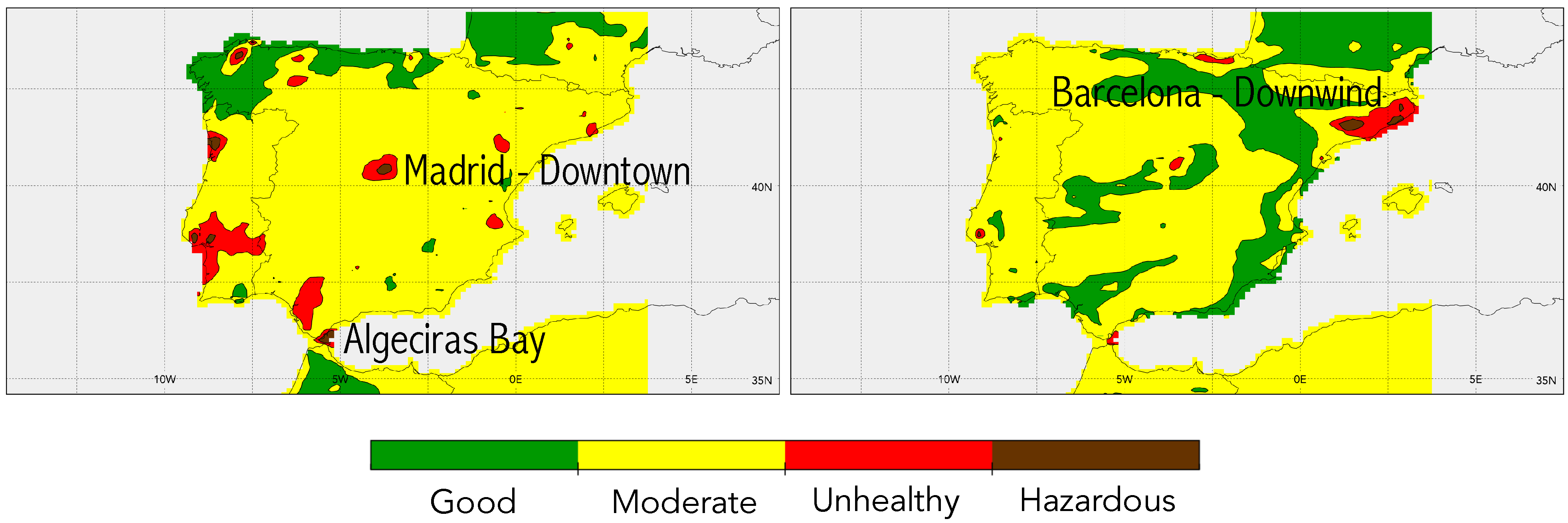
Figure 5 shows the Air Quality Index (AQI) in the IP (estimated from EPA Air Quality Index [82]) in order to assess the most critical areas in the target domain regarding air pollution. In this index, the concentrations that correspond to an AQI value of 100 are those established as the standards of the European Union, compiled in Directive 2008/50/EC. The election of the AQI in this contribution is not critical, since only the areas with the poorest air quality are searched to calculate the source contribution at those particular locations.

The AQI has been estimated individually for all pollutants with regulatory values included in this contribution (O${}_3$, NO${}_2$, SO${}_2$, PM${}_{10}$, and PM${}_{2.5}$) and the AQI${}_{total}$ (shown in Figure 5) has been estimated as the highest value among all individual indexes. During the summer and winter periods, air quality was hazardous in the two largest Spanish cities (Madrid and Barcelona) and the industrial-harbor area of Algeciras Bay, located in southern Spain (Figure 5). Therefore, this section is devoted to the analysis of the source apportionment at these locations in order to shed some light on the causes of the strategy to abate those pollutants. For that, the point with the worst air quality in a domain of 100 km${}^2$, centred over Madrid, Barcelona, and Algeciras, respectively, has been selected for further analysis.

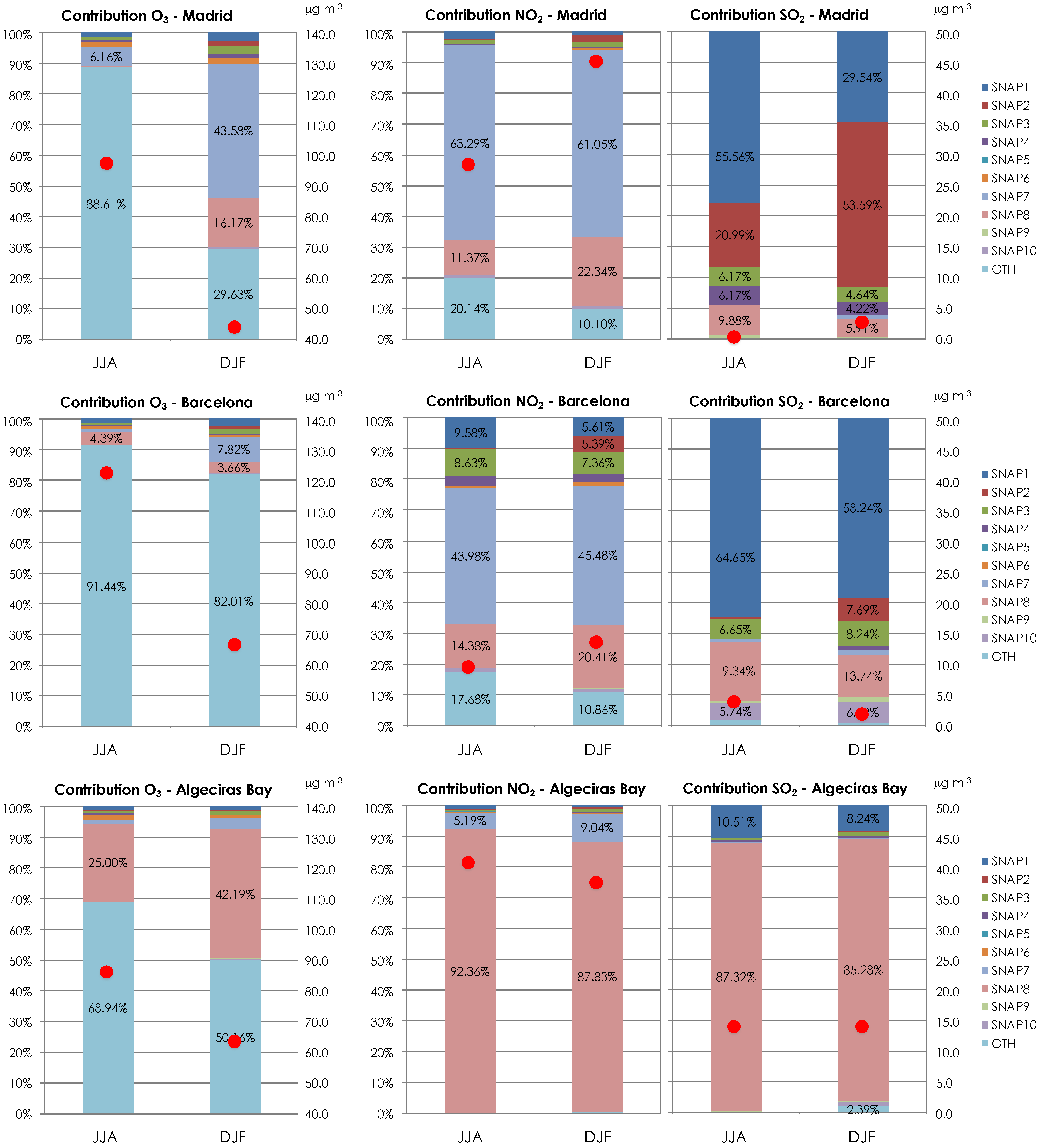
For gas-phase pollutants, Figure 6 (left) indicates that most of summertime tropospheric O${}_3$ comes from the “Other” sector at all the three sites. This “Other” contribution is not estimated by zeroing-out any emission sector, but estimated as the difference between the BC and the addition of all anthropogenic sources. Therefore, it includes the contribution of different processes (e.g., long-range transport, background levels, stratosphere–troposphere exchange, etc.).

During summer (winter), this contribution can be as large as 88% (30%) in Madrid, 91% (82%) in Barcelona. and 69% (50%) in Algeciras Bay. These numbers are in agreement with previous works. For instance, the background values contribute with more than 50% to the O${}_3$ concentration measured in the westernmost region of the IP [83]. Moreover, the importance of intercontinental ozone transport in the ground levels of ozone over Europe has been highlighted [84], and can be as high as 10–16 ppb (20–32 $\mathsf{\mu }$g m${}^{-3}$). In Barcelona and the Algeciras Bay, the anthropogenic sector contributing most to tropospheric O${}_3$ levels is SNAP8 (other mobile sources), especially related to shipping emissions in the area. SNAP8 adds up 4% (25%) and 4% (42%) of summer and wintertime O${}_3$, respectively, in Barcelona (Algeciras). These results are in agreement with those of the literature [85,86]. These works find out that shipping emissions increase ground levels of summer tropospheric O${}_3$ by 5 to 10% in the Mediterranean sea. This may be caused by the large NO${}_2$ emissions of ships, which can enhance the production of ozone [87]. Last, SNAP7 (road traffic) has a limited contribution to summertime O${}_3$ levels in Madrid and Barcelona, around 8%, which is in a strong agreement with previous works [88].

With respect to NO${}_2$ (Figure 6, center), on-road traffic (SNAP7) is the sector with the highest contribution to the surface levels of NO${}_2$ in Madrid and Barcelona (over 60% in Madrid and over 44% in Barcelona for both seasons), followed by SNAP8 (other mobile sources). While for Barcelona, it is the shipping and maritime activity that contributes most to SNAP8 (being responsible for 14% and 20% of summer and winter NO${}_2$ levels in the city), in Madrid, the contribution of SNAP8 (11% in summer and 22% in winter) comes mainly from the activity of the Madrid airport. In Algeciras, around 90% of NO${}_2$ levels can be attributed to the shipping sector, both in summertime and wintertime. The contribution of SNAP8 is very similar in Algeciras Bay for SO${}_2$ levels (the source apportionment indicates that over 85% of SO${}_2$ mean levels in Algeciras come from SNAP8) (Figure 6, right). However, in the city of Madrid, most of the summer (winter) SO${}_2$ has an origin in combustion during energy-generation activities (SNAP1): 56% (30%) of monthly means for summertime (wintertime), followed by non-industrial combustion plants, including private wood combustion—SNAP2—(21%/54% of summer/winter levels). In Barcelona, SNAP1 is also responsible for around 60% of SO${}_2$ levels, with a limited contribution of shipping emissions (19% for summertime and 14% during winter) and agriculture—SNAP10—(around 6% for both seasons). It should be highlighted that the levels of SO${}_2$ in the urban areas of Madrid and Barcelona are very low, with mean monthly concentrations under 5 $\mathsf{\mu }$g m${}^{-3}$.

Figure 7 indicates the results regarding the contribution of each SNAP sector to the daily mean levels of PM${}_{2.5}$ (left) and PM${}_{10}$ (right). The most important contributor to PM${}_{2.5}$ and PM${}_{10}$ concentrations in Madrid, Barcelona, and Algeciras is the sector “Other”, highlighting the importance of external sources to the domain during summertime (e.g., Saharan dust transport). In this sense, the outside contribution represents 72% (73%), 59% (63%), and 52% (57%) of summertime PM${}_{2.5}$ (PM${}_{10}$) levels in Madrid, Barcelona, and Algeciras, respectively. However, this contribution is much lower for wintertime, when the external contribution accounts for only 16% (7%), 31% (29%), and 35% (29%) of PM${}_{2.5}$ (PM${}_{10}$) levels at the aforementioned sites. The fact that the PM${}_{10}$ contribution is larger than PM${}_{2.5}$ for summertime, but lower for wintertime, points to an important role of dust outbreaks over the IP during the summer months, as aforementioned [25,73].

Agriculture (SNAP10) effects on particulate matter levels are much larger in wintertime than during summertime. SNAP10 has a larger contribution to summer particles in Barcelona (18% for PM${}_{2.5}$ and 16% for PM${}_{10}$) than in the case of Madrid (6% for PM${}_{2.5}$ and PM${}_{10}$) or Algeciras (14% and 10% for PM${}_{2.5}$ and PM${}_{10}$, respectively). These contributions increase notably for wintertime, with agriculture being the most important contributor to wintertime PM${}_{2.5}$ and PM${}_{10}$ levels in Madrid (49% and 52%, respectively) and Barcelona (39% and 40%).

Combustion in energy and transformation industries (SNAP1) also notably contributes to particle levels in the city of Madrid (PM${}_{2.5}$: 18% for summer and 13% for winter; PM${}_{10}$: 15% and 12% in summer and winter, in that order), Barcelona (PM${}_{2.5}$: 10% for summer and 11% for winter; PM${}_{10}$: 11% and 10% in summer and winter, respectively), and Algeciras (PM${}_{2.5}$: 7% and 1% for summer/winter; PM${}_{10}$: 10% and 9% in summer and winter, in that order). On-road traffic (SNAP7) is only noticeable for wintertime PM${}_{2.5}$(PM${}_{10}$) concentrations, being 11% (13%), 8% (10%), and 5% (8%) in Madrid, Barcelona, and Algeciras, while the contributions of SNAP8 (other mobile sources) are very high in Algeciras, being the second largest contributor for particulate matter both in summer (18% for PM${}_{2.5}$ and PM${}_{10}$) and winter (23% and 19% for PM${}_{2.5}$ and PM${}_{10}$, respectively), due to the presence of important harbor/industrial activity in the area [89,90]. Over a coastal area such as Barcelona, the estimated contribution of harbor emissions to the urban background reached 9–12% for PM${}_{10}$ and 11–15% for PM${}_{2.5}$ [91]. Our results are in agreement with those numbers (despite being slightly lower), since the estimations of the contribution of SNAP8 to PM${}_{2.5}$ (PM${}_{10}$) background levels in Barcelona is around 4–6%. This contribution is linked both to primary emissions from fuel oil combustion but also to the formation of secondary aerosols from gas-phase precursors.

3.4. Response of Air Quality Exceedances to Zeroed-Out Emissions

It is important to characterize the contribution of each emitting sector to air pollution not only from the point of view of the percent contribution to mean air quality levels, but also to attribute the role of those sources in the exceedances of limit values for the protection of human health. In this sense,

Table 6. Variation in the number of exceedances over the entire IP when zeroing-out the different SNAP sectors (base case minus zeroed-out SNAP sector simulation).

Summer	Summer 2011
	Concentration	w/o SNAP
Pollutant	Limit value	Zero-out sector	N exc. BC	N. exc. noSNAP
O${}_3$	Objective value for O${}_3$, 120 $\mathsf{\mu }$g m${}^{-3}$, 8 h	SNAP7	23	16
		SNAP8		18
NO${}_2$	Limit value for NO${}_2$, 200 $\mathsf{\mu }$g m${}^{-3}$, 1 h	SNAP8	2	0
SO${}_2$	Limit value for SO${}_2$, 125 $\mathsf{\mu }$g m${}^{-3}$, 1 day	SNAP1	8	5
		SNAP8		2
PM${}_{10}$	Limit value for PM${}_{10}$, 50 $\mathsf{\mu }$g m${}^{-3}$, 1 day	SNAP1	18	13
		SNAP8		16
		SNAP10		16
Winter	December 2011
	Concentration	w/o SNAP
Pollutant	Limit value	Zero-out sector	N exc. BC	N. exc. noSNAP
O${}_3$	Objective value for O${}_3$, 120 $\mathsf{\mu }$g m${}^{-3}$, 8 h	SNAP7	0	0
NO${}_2$	Limit value for NO${}_2$, 200 $\mathsf{\mu }$g m${}^{-3}$, 1 h	SNAP8	0	0
SO${}_2$	Limit value for SO${}_2$, 125 $\mathsf{\mu }$g m${}^{-3}$, 1 day	SNAP1	0	0
		SNAP8		0
PM${}_{10}$	Limit value for PM${}_{10}$, 50 $\mathsf{\mu }$g m${}^{-3}$, 1 day	SNAP4	27	22
		SNAP7		26
		SNAP10		21

summarizes the contribution over the entire IP of each SNAP sector (only for those sectors with significant variations with respect to the BC) to the number of exceedances of different target values selected: objective value for O${}_3$, 120 $\mathsf{\mu }$g m${}^{-3}$, 8 h; limit value for NO${}_2$, 200 $\mathsf{\mu }$g m${}^{-3}$, 1 h, not to be exceeded (n.t.b.e.) more than 3 times a calendar year; limit value for SO${}_2$, 125 $\mathsf{\mu }$g m${}^{-3}$, 1 day, n.t.b.e. more than 3 times a calendar year; limit value for PM${}_{10}$, 50 $\mathsf{\mu }$g m${}^{-3}$, 1 day, n.t.b.e. more than 35 times a calendar year. Additionally, the limit value for PM${}_{2.5}$, 25 $\mathsf{\mu }$g m${}^{-3}$, 1 calendar year, was explored, but as we have only simulated summer and winter periods, this latter limit value cannot be assessed.

With respect to the exceedance of the target, limit, and threshold values set in the Directive 2008/50/EC, Table 6 indicates a clear improvement in the O${}_3$ objective value (120 $\mathsf{\mu }$g m${}^{-3}$, max. 8 h) when zeroing-out the on-road traffic emissions (SNAP7) for summertime (days with exceedances reduce from 23 to 16 in summer; no exceedances are simulated for winter in the base case); however, this management strategy is hard to take into practice because of the socio-economical implications of road traffic reduction. Moreover, other mobile sources (SNAP8) contribute to 5 days with exceedances of the object value for O${}_3$ (23 days in BC vs. 18 in noSNAP8).

Additionally, other mobile sources (SNAP8) is the sector causing most of the exceedances of the limit values related to NO${}_2$ (200 $\mathsf{\mu }$g m${}^{-3}$, 1 h) and SO${}_2$ (125 $\mathsf{\mu }$g m${}^{-3}$, daily mean) over the IP (playing also a role on PM${}_{10}$ exceedances). In this sense, SNAP8 causes the two exceedances of the limit value of modeled NO${}_2$ and is responsible for six out of the eight exceedances of the daily limit value for SO${}_2$ (125 $\mathsf{\mu }$g m${}^{-3}$) over the domain for summertime (no values over the limit value for NO${}_2$ or SO${}_2$ are modeled during wintertime). SO${}_2$ concentrations over the limit value are found over the Algeciras Bay, and are caused mainly from the contribution of the high sulphur emissions coming from ship fuels. It is noteworthy that the contribution of shipping emissions to the exceedances of the limit value for PM${}_{10}$ is not as large as for SO${}_2$ (in agreement with [92]), since there are components of particulate matter from shipping not directly affected by the sulphur content in the fuels. In this sense, just 2 of the 18 summertime exceedances of the daily mean 50-$\mathsf{\mu }$g m${}^{-3}$ limit value for PM${}_{10}$ are caused by SNAP8 (no exceedances of the PM${}_{10}$ limit value are caused by other mobile sources in wintertime). For particles, combustion in energy generation (SNAP1) is responsible of 5 out of the 18 (27) exceedances of the PM${}_{10}$ limit value for summertime (wintertime), while agriculture (SNAP10) contributes to 2 (6) exceedances of the daily mean 50-$\mathsf{\mu }$g m${}^{-3}$ limit value for summertime (wintertime).

4. Discussion and Conclusions

Efficient air quality management requires an accurate identification of pollution sources and of their individual contributions to the ambient pollutant concentrations. To this end, the zero-out methodology has been proposed and applied for the apportionment of atmospheric pollutants in the IP. This method is based on the application of WRF + CHIMERE chemistry transport model coupled to EMEP emissions.

Regarding tropospheric O${}_3$, on-road traffic is the only anthropogenic sector with a noticeable contribution to maximum O${}_3$ levels during summertime (6%) and is responsible for 7 summer days with exceedances in the objective value of 120 $\mathsf{\mu }$g m${}^{-3}$ (max. 8-hr mean) established by the 2008/50/EC directive. These results are in agreement with those of the scientific literature [37,62]. These authors found out that the on-road transport sector (SNAP7) was the largest overall anthropogenic source sector contributing to July 2011 O${}_3$ concentrations in Europe, with non-road transport (SNAP8) contributions ranking second, as in our case (2% contribution to summertime maximum O${}_3$ levels and five exceedances of the objective value). An analogous analysis can be completed for SNAP8 (other mobile sources) with respect to NO${}_2$, with this sector prevailing in the contribution to mean ground-level concentrations during summertime and contributing to the two exceedances of the limit value for the protection of human health for NO${}_2$ (200 $\mathsf{\mu }$g m${}^{-3}$, 1 h) modeled over the IP. The importance of this sector in the IP is larger closer to the major shipping routes and main harbors, with relative contributions varying from 10 to 50% depending on the pollutant (the lowest contribution for particulate matter, the largest for SO${}_2$ and NO${}_2$).

Last, the other anthropogenic sector with a noticeable impact is agriculture. Removing agriculture emissions (SNAP10) contributes to a decrease in PM levels and a simultaneous increase of SO${}_2$ concentrations. The reduction of the most important source contributing to ammonia emissions controls the formation of ammonium sulphate. Therefore, reducing the levels of ammonia permits the SO${}_2$ to remain in the gas phase. Agriculture contributes to the limit value for the protection of human health regarding PM${}_{10}$ (50 $\mathsf{\mu }$g m${}^{-3}$, daily mean) with 2 exceedances out of 18, while this number increases to 6 out of 27 wintertime exceedances.

With respect to the temporal pattern, in general, the source contribution does not exhibit a strong seasonality, except for particulate mater under the “Other” sector, which includes the external contribution to particle levels. Despite this seasonal behaviour for particulate matter, both gas-phase pollutants and particles exhibit a strong spatial uniformity, since background concentrations in the modeling system are provided by coarse resolution chemistry/climate models that do not allow for a sharp gradient in the background concentrations.

The external contribution of particles to the “Other” sector is mainly composed of mineral matter from Saharan dust. The fact that the boundary contributions to PM${}_{10}$ are larger than for PM${}_{2.5}$ for summertime, but lower for wintertime, points to an important role of dust outbreaks over the IP during the summer months, which contributes mainly with large particles. These results are in line with those of Karachamdani et al. [37] for 16 European cities, who indicate that the boundary condition contributions for the Mediterranean cities are larger than for other European cities, ranging from about 40–50% during summertime to 10–15% in wintertime, because those Mediterranean cities were largely influenced by the long-range transport of dust emissions from northern Africa in the summer months.

Locally, the IP undergoes diverse problems related to air quality both during summer and winter. Focusing on the most polluted areas of the target domain (the cities of Madrid, Barcelona, and Algeciras Bay), the impact of road transport (SNAP7) emissions is high for NO${}_2$ ground levels over largely populated areas (Madrid or Barcelona areas), but the concentration of this pollutant is dominated by other mobile sources (such as maritime or airport emissions included in SNAP8). Over coastal areas of the target domain, a poor air quality caused by large NO${}_2$ concentrations can be attributed to shipping routes. In this sense, Merico et al. [87] also highlight the influence of harbor and shipping emissions on air quality of the nearby coastal areas of the Mediterranean.

For SO${}_2$, energy generation (SNAP1) controls the mean levels of this pollutant over most of the areas considered. Valverde et al. [70] indicate that the contribution of power plants to the surface concentration of SO${}_2$ occurs mainly close to the source (<20 km) related to a fumigation process when the emission injection takes place within the planetary boundary layer, but those plumes can reach long distances (>250 km) from the sources.

In the Algeciras Bay, maritime emissions largely contribute to the levels of SO${}_2$. The implementation of low-sulphur fuels in shipping may contribute to substantially reducing the number of exceedances of the limit values for the protection of human health and to reduce several pathologies such as cardiovascular and cancer deaths, childhood asthma, or premature mortality and morbidity [93]. Summertime PM${}_{10}$ and PM${}_{2.5}$ levels are dominated by the external contribution of Saharan dust, while for wintertime, agriculture can have a dominant position in Madrid and Barcelona. The important contribution of agriculture to PM levels was highlighted by Lelieveld et al. [94], who stated that this sector is the largest contributor to PM${}_{2.5}$ levels in Europe.

Hence, this evaluated contribution has allowed us to identify which sectors contribute most to air pollution problems in the IP. However, it should be borne in mind that the uncertainties associated with several factors (principally, the boundary conditions in the CTMs and emission inventories) can condition the accuracy of the obtained results [37,95]. For instance, Jiménez et al. [17] analyze the impact of initial and boundary conditions over the Levantine coast of the IP, indicating that, despite the influence of initial condition reduces with the spin-up time (a 48-h spin-up time is sufficient to reduce the impact factor of initial conditions to 10% or less), the importance of having accurate boundary conditions becomes essential, since its influence on the results increases with the time of the simulation, reaching up to 5 $\mathsf{\mu }$g m${}^{-3}$ for certain pollutants. With respect to the emission inventories, Baldasano et al. [96] point to industrial facilities as the main sources of uncertainties in emission inventories over the target area.

Nonetheless, this work can provide a very useful contribution to a better understanding of the sensitivity of air pollutants in a complex area such as the IP, and can provide valuable information for the design of mitigation strategies or plans that lead to an improvement in European air quality and the attainment of the SDG over the target area.

References

1. United Nations. Transforming Our World: The 2030 Agenda for Sustainable Development (A/RES/70/1); UN General Assembly: New York, NY, USA, 2015. [Google Scholar]
2. Tsai, W.T.; Lin, Y.Q. Trend Analysis of Air Quality Index (AQI) and Greenhouse Gas (GHG) Emissions in Taiwan and Their Regulatory Countermeasures. Environments 2021, 8, 29. [Google Scholar] [CrossRef]
3. Kahraman, A.C.; Sivri, N. Comparison of metropolitan cities for mortality rates attributed to ambient air pollution using the AirQ model. Environ. Sci. Pollut. Res. 2022, 29, 1. [Google Scholar] [CrossRef] [PubMed]
4. Osman, T.; Kenawy, E.; Abdrabo, K.I.; Shaw, D.; Alshamndy, A.; Elsharif, M.; Salem, M.; Alwetaishi, M.; Aly, R.M.; Elboshy, B. Voluntary Local Review Framework to Monitor and Evaluate the Progress towards Achieving Sustainable Development Goals at a City Level: Buraidah City, KSA and SDG11 as A Case Study. Sustainability 2021, 13, 9555. [Google Scholar] [CrossRef]
5. Pateman, R.; Tuhkanen, H.; Cinderby, S. Citizen Science and the Sustainable Development Goals in Low and Middle Income Country Cities. Sustainability 2021, 13, 9534. [Google Scholar] [CrossRef]
6. Cuvelier, C.; Thunis, P.; Vautard, R.; Amann, M.; Bessagnet, B.; Bedogni, M.; Berkowicz, R.; Brandt, J.; Brocheton, F.; Builtjes, P.; et al. CityDelta: A model intercomparison study to explore the impact of emission reductions in European cities in 2010. Atmos. Environ. 2007, 41, 189–207. [Google Scholar] [CrossRef]
7. Ballester, F.; Medina, S.; Boldo, E.; Goodman, P.; Neuberger, M.; Iñiguez, C.; Künzli, N. Reducing ambient levels of fine particulates could substantially improve health: A mortality impact assessment for 26 European cities. J. Epidemiol. Community Health 2008, 62, 98–105. [Google Scholar] [CrossRef]
8. Pope, C.A.; Ezzati, M.; Dockery, D.W. Fine-Particulate Air Pollution and Life Expectancy in the United States. N. Engl. J. Med. 2009, 360, 376–386. [Google Scholar] [CrossRef] [Green Version]
9. Beelen, R.; Raaschou-Nielsen, O.; Stafoggia, M.; Andersen, Z.J.; Weinmayr, G.; Hoffmann, B.; Wolf, K.; Samoli, E.; Fischer, P.; Nieuwenhuijsen, M.; et al. Effects of long-term exposure to air pollution on natural-cause mortality: An analysis of 22 European cohorts within the multicentre ESCAPE project. Lancet 2014, 383, 785–795. [Google Scholar] [CrossRef]
10. Héroux, M.E.; Anderson, H.R.; Atkinson, R.; Brunekreef, B.; Cohen, A.; Forastiere, F.; Hurley, F.; Katsouyanni, K.; Krewski, D.; Krzyzanowski, M.; et al. Quantifying the health impacts of ambient air pollutants: Recommendations of a WHO/Europe project. Int. J. Public Health 2015, 60, 619–627. [Google Scholar] [CrossRef] [Green Version]
11. Tarín-Carrasco, P.; Im, U.; Geels, C.; Palacios-Peña, L.; Jiménez-Guerrero, P. Contribution of fine particulate matter to present and future premature mortality over Europe: A non-linear response. Environ. Int. 2021, 153, 106517. [Google Scholar] [CrossRef]
12. Guzmán, P.; Tarín-Carrasco, P.; Morales-Suárez-Varela, M.; Jiménez-Guerrero, P. Effects of air pollution on dementia over Europe for present and future climate change scenarios. Environ. Res. 2022, 204, 112012. [Google Scholar] [CrossRef]
13. Im, U.; Brandt, J.; Geels, C.; Hansen, K.M.; Christensen, J.H.; Andersen, M.S.; Solazzo, E.; Kioutsioukis, I.; Alyuz, U.; Balzarini, A.; et al. Assessment and economic valuation of air pollution impacts on human health over Europe and the United States as calculated by a multi-model ensemble in the framework of AQMEII3. Atmos. Chem. Phys. 2018, 18, 5967–5989. [Google Scholar] [CrossRef] [PubMed] [Green Version]
14. Tarín-Carrasco, P.; Morales-Suárez-Varela, M.; Im, U.; Brandt, J.; Palacios-Peña, L.; Jiménez-Guerrero, P. Isolating the climate change impacts on air-pollution-related-pathologies over central and southern Europe—A modelling approach on cases and costs. Atmos. Chem. Phys. 2019, 19, 9385–9398. [Google Scholar] [CrossRef] [Green Version]
15. Monteiro, A.; Carvalho, A.; Ribeiro, I.; Scotto, M.; Barbosa, S.; Alonso, A.; Baldasano, J.; Pay, M.; Miranda, A.; Borrego, C. Trends in ozone concentrations in the Iberian Peninsula by quantile regression and clustering. Atmos. Environ. 2012, 56, 184–193. [Google Scholar] [CrossRef] [Green Version]
16. Baldasano, J.; Pay, M.; Jorba, O.; Gassó, S.; Jiménez-Guerrero, P. An annual assessment of air quality with the CALIOPE modeling system over Spain. Sci. Total Environ. 2011, 409, 2163–2178. [Google Scholar] [CrossRef] [Green Version]
17. Jiménez, P.; Parra, R.; Baldasano, J.M. Influence of initial and boundary conditions for ozone modeling in very complex terrains: A case study in the northeastern Iberian Peninsula. Environ. Model. Softw. 2007, 22, 1294–1306. [Google Scholar] [CrossRef]
18. Vivanco, M.G.; Palomino, I.; Vautard, R.; Bessagnet, B.; Martín, F.; Menut, L.; Jiménez, S. Multi-year assessment of photochemical air quality simulation over Spain. Environ. Model. Softw. 2009, 24, 63–73. [Google Scholar] [CrossRef]
19. Borge, R.; López, J.; Lumbreras, J.; Narros, A.; Rodríguez, E. Influence of boundary conditions on CMAQ simulations over the Iberian Peninsula. Atmos. Environ. 2010, 44, 2681–2695. [Google Scholar] [CrossRef]
20. Pay, M.T.; Jiménez-Guerrero, P.; Baldasano, J.M. Assessing sensitivity regimes of secondary inorganic aerosol formation in Europe with the CALIOPE-EU modeling system. Atmos. Environ. 2012, 51, 146–164. [Google Scholar] [CrossRef] [Green Version]
21. Vedrenne, M.; Borge, R.; Lumbreras, J.; Conlan, B.; Rodríguez, M.E.; de Andrés, J.M.; de la Paz, D.; Pérez, J.; Narros, A. An integrated assessment of two decades of air pollution policy making in Spain: Impacts, costs and improvements. Sci. Total Environ. 2015, 527–528, 351–361. [Google Scholar] [CrossRef] [Green Version]
22. Palacios-Peña, L.; Baró, R.; Guerrero-Rascado, J.L.; Alados-Arboledas, L.; Brunner, D.; Jiménez-Guerrero, P. Evaluating the representation of aerosol optical properties using an online coupled model over the Iberian Peninsula. Atmos. Chem. Phys. 2017, 17, 277–296. [Google Scholar] [CrossRef] [Green Version]
23. Guevara, M.; Martínez, F.; Arévalo, G.; Gassó, S.; Baldasano, J.M. An improved system for modelling Spanish emissions: HERMESv2.0. Atmos. Environ. 2013, 81, 209–221. [Google Scholar] [CrossRef]
24. Nunes, R.A.O.; Alvim-Ferraz, M.C.M.; Martins, F.G.; Calderay-Cayetano, F.; Durán-Grados, V.; Moreno-Gutiérrez, J.; Jalkanen, J.P.; Hannuniemi, H.; Sousa, S.I.V. Shipping emissions in the Iberian Peninsula and the impacts on air quality. Atmos. Chem. Phys. 2020, 20, 9473–9489. [Google Scholar] [CrossRef]
25. Querol, X.; Pey, J.; Pandolfi, M.; Alastuey, A.; Cusack, M.; Pérez, N.; Moreno, T.; Viana, M.; Mihalopoulos, N.; Kallos, G.; et al. African dust contributions to mean ambient PM10 mass-levels across the Mediterranean Basin. Atmos. Environ. 2009, 43, 4266–4277. [Google Scholar] [CrossRef]
26. Carvalho, A.; Monteiro, A.; Solman, S.; Miranda, A.; Borrego, C. Climate-driven changes in air quality over Europe by the end of the 21st century, with special reference to Portugal. Environ. Sci. Policy 2010, 13, 445–458. [Google Scholar] [CrossRef] [Green Version]
27. Jiménez-Guerrero, P.; Montávez, J.P.; Gómez-Navarro, J.J.; Jerez, S.; Lorente-Plazas, R. Impacts of climate change on ground level gas-phase pollutants and aerosols in the Iberian Peninsula for the late XXI century. Atmos. Environ. 2012, 55, 483–495. [Google Scholar] [CrossRef]
28. Jiménez-Guerrero, P.; Gómez-Navarro, J.J.; Baró, R.; Lorente, R.; Ratola, N.; Montávez, J.P. Is there a common pattern of future gas-phase air pollution in Europe under diverse climate change scenarios? Clim. Change 2013, 121, 661–671. [Google Scholar] [CrossRef]
29. Jiménez-Guerrero, P.; Jerez, S.; Montávez, J.P.; Trigo, R.M. Uncertainties in future ozone and PM10 projections over Europe from a regional climate multiphysics ensemble. Geophys. Res. Lett. 2013, 40, 5764–5769. [Google Scholar] [CrossRef]
30. Monteiro, A.; Sá, E.; Fernandes, A.; Gama, C.; Sorte, S.; Borrego, C.; Lopes, M.; Russo, M.A. How healthy will be the air quality in 2050? Air Qual. Atmos. Health 2018, 11, 353–362. [Google Scholar] [CrossRef] [Green Version]
31. Vautard, R.; Colette, A.; van Meijgaard, E.; Meleux, F.; van Oldenborgh, G.J.; Otto, F.; Tobin, I.; Yiou, P. Attribution of Wintertime Anticyclonic Stagnation Contributing to Air Pollution in Western Europe. Bull. Am. Meteorol. Soc. 2018, 99, S70–S75. [Google Scholar] [CrossRef] [Green Version]
32. Yarwood, G.; Emery, C.; Jung, J.; Nopmongcol, U.; Sakulyanontvittaya, T. A method to represent ozone response to large changes in precursor emissions using high-order sensitivity analysis in photochemical models. Geosci. Model Dev. 2013, 6, 1601–1608. [Google Scholar] [CrossRef] [Green Version]
33. Pisoni, E.; Albrecht, D.; Mara, T.; Rosati, R.; Tarantola, S.; Thunis, P. Application of uncertainty and sensitivity analysis to the air quality SHERPA modelling tool. Atmos. Environ. 2018, 183, 84–93. [Google Scholar] [CrossRef]
34. Koo, B.; Wilson, G.M.; Morris, R.E.; Dunker, A.M.; Yarwood, G. Comparison of Source Apportionment and Sensitivity Analysis in a Particulate Matter Air Quality Model. Environ. Sci. Technol. 2009, 43, 6669–6675. [Google Scholar] [CrossRef] [PubMed]
35. Kranenburg, R.; Segers, A.J.; Hendriks, C.; Schaap, M. Source apportionment using LOTOS-EUROS: Module description and evaluation. Geosci. Model Dev. 2013, 6, 721–733. [Google Scholar] [CrossRef] [Green Version]
36. Clappier, A.; Belis, C.A.; Pernigotti, D.; Thunis, P. Source apportionment and sensitivity analysis: Two methodologies with two different purposes. Geosci. Model Dev. 2017, 10, 4245–4256. [Google Scholar] [CrossRef] [Green Version]
37. Karamchandani, P.; Long, Y.; Pirovano, G.; Balzarini, A.; Yarwood, G. Source-sector contributions to European ozone and fine PM in 2010 using AQMEII modeling data. Atmos. Chem. Phys. 2017, 17, 5643–5664. [Google Scholar] [CrossRef] [Green Version]
38. Wang, L.; Wei, Z.; Wei, W.; Fu, J.S.; Meng, C.; Ma, S. Source apportionment of PM2.5 in top polluted cities in Hebei, China using the CMAQ model. Atmos. Environ. 2015, 122, 723–736. [Google Scholar] [CrossRef]
39. Huang, Y.; Deng, T.; Li, Z.; Wang, N.; Yin, C.; Wang, S.; Fan, S. Numerical simulations for the sources apportionment and control strategies of PM2.5 over Pearl River Delta, China, part I: Inventory and PM2.5 sources apportionment. Sci. Total Environ. 2018, 634, 1631–1644. [Google Scholar] [CrossRef]
40. Baker, K.; Woody, M.; Tonnesen, G.; Hutzell, W.; Pye, H.; Beaver, M.; Pouliot, G.; Pierce, T. Contribution of regional-scale fire events to ozone and PM2.5 air quality estimated by photochemical modeling approaches. Atmos. Environ. 2016, 140, 539–554. [Google Scholar] [CrossRef]
41. Han, X.; Zhang, M.; Zhu, L.; Skorokhod, A. Assessment of the impact of emissions reductions on air quality over North China Plain. Atmos. Pollut. Res. 2016, 7, 249–259. [Google Scholar] [CrossRef]
42. Klemp, J.B.; Skamarock, W.C.; Dudhia, J. Conservative Split-Explicit Time Integration Methods for the Compressible Nonhydrostatic Equations. Mon. Weather Rev. 2007, 135, 2897–2913. [Google Scholar] [CrossRef] [Green Version]
43. Skamarock, W.C.; Klemp, J.B.; Dudhia, J.; Gill, D.O.; Barker, D.M.; Wang, W.; Powers, J.G. A Description of the Advanced Research WRF Version 3; note-475+ STR; NCAR Technical Report: Boulder, CO, USA, 2008. [Google Scholar]
44. Dee, D.P.; Uppala, S.M.; Simmons, A.J.; Berrisford, P.; Poli, P.; Kobayashi, S.; Andrae, U.; Balmaseda, M.A.; Balsamo, G.; Bauer, P.; et al. The ERA-Interim reanalysis: Configuration and performance of the data assimilation system. Q. J. R. Meteorol. Soc. 2011, 137, 553–597. [Google Scholar] [CrossRef]
45. Menut, L.; Bessagnet, B.; Khvorostyanov, D.; Beekmann, M.; Blond, N.; Colette, A.; Coll, I.; Curci, G.; Foret, G.; Hodzic, A.; et al. CHIMERE 2013: A model for regional atmospheric composition modelling. Geosci. Model Dev. 2013, 6, 981–1028. [Google Scholar] [CrossRef] [Green Version]
46. Derognat, C.; Beekmann, M.; Baeumle, M.; Martin, D.; Schmidt, H. Effect of biogenic volatile organic compound emissions on tropospheric chemistry during the Atmospheric Pollution Over the Paris Area (ESQUIF) campaign in the Ile-de-France region. J. Geophys. Res. 2003, 108, 8560. [Google Scholar] [CrossRef]
47. Hong, S.; Lim, J.O.J. The WRF Single-Moment 6-Class Microphysics Scheme (WSM6). Asia-Pac. J. Atmos. Sci. 2006, 42, 129–151. [Google Scholar]
48. Hong, S.Y.; Noh, Y.; Dudhia, J. A New Vertical Diffusion Package with an Explicit Treatment of Entrainment Processes. Mon. Weather Rev. 2006, 134, 2318–2341. [Google Scholar] [CrossRef] [Green Version]
49. Nenes, A.; Pandis, S.N.; Pilinis, C. ISORROPIA: A New Thermodynamic Equilibrium Model for Multiphase Multicomponent Inorganic Aerosols. Aquat. Geochem. 1998, 4, 123–152. [Google Scholar] [CrossRef]
50. Collins, W.D.; Rasch, P.J.; Boville, B.A.; Hack, J.J.; McCaa, J.R.; Williamson, D.L.; Kiehl, J.T.; Briegleb, B.; Bitz, C.; Lin, S.J.; et al. Description of the NCAR Community Atmosphere Model (CAM 3.0); Note NCAR/TN-464+ STR; NCAR Technical Report; NCAR: Boulder, CO, USA, 2004; Volume 226, pp. 1326–1334. [Google Scholar]
51. Bessagnet, B.; Menut, L.; Curci, G.; Hodzic, A.; Guillaume, B.; Liousse, C.; Moukhtar, S.; Pun, B.; Seigneur, C.; Schulz, M. Regional modeling of carbonaceous aerosols over Europe—Focus on secondary organic aerosols. J. Atmos. Chem. 2008, 61, 175–202. [Google Scholar] [CrossRef]
52. Chen, F.; Dudhia, J. Coupling an Advanced Land Surface-Hydrology Model with the Penn State-NCAR MM5 Modeling System. Part I: Model Implementation and Sensitivity. Mon. Weather Rev. 2001, 129, 569–585. [Google Scholar] [CrossRef] [Green Version]
53. Kain, J.S. The Kain-Fritsch convective parameterization: An update. J. Appl. Meteorol. 2004, 43, 170–181. [Google Scholar] [CrossRef] [Green Version]
54. Vestreng, V.; Ntziachristos, L.; Semb, A.; Reis, S.; Isaksen, I.S.; Tarrasón, L. Evolution of NOxemissions in Europe with focus on road transport control measures. Atmos. Chem. Phys. 2009, 9, 1503–1520. [Google Scholar] [CrossRef] [Green Version]
55. Guenther, A.; Karl, T.; Harley, P.; Wiedinmyer, C.; Palmer, P.I.; Geron, C. Estimates of global terrestrial isoprene emissions using MEGAN (Model of Emissions of Gases and Aerosols from Nature). Atmos. Chem. Phys. 2006, 6, 3181–3210. [Google Scholar] [CrossRef] [Green Version]
56. Folberth, G.A.; Hauglustaine, D.A.; Lathière, J.; Brocheton, F. Interactive chemistry in the Laboratoire de Météorologie Dynamique general circulation model: Model description and impact analysis of biogenic hydrocarbons on tropospheric chemistry. Atmos. Chem. Phys. 2006, 6, 2273–2319. [Google Scholar] [CrossRef] [Green Version]
57. Szopa, S.; Foret, G.; Menut, L.; Cozic, A. Impact of large scale circulation on European summer surface ozone and consequences for modelling forecast. Atmos. Environ. 2009, 43, 1189–1195. [Google Scholar] [CrossRef]
58. Jiménez-Guerrero, P.; Ratola, N. Influence of the North Atlantic oscillation on the atmospheric levels of benzo[a]pyrene over Europe. Clim. Dyn. 2021, 57, 1173–1186. [Google Scholar] [CrossRef]
59. Borge, R.; Lumbreras, J.; Vardoulakis, S.; Kassomenos, P.; Rodríguez, E. Analysis of long-range transport influences on urban PM10 using two-stage atmospheric trajectory clusters. Atmos. Environ. 2007, 41, 4434–4450. [Google Scholar] [CrossRef]
60. Salvador, P.; Artíñano, B.; Molero, F.; Viana, M.; Pey, J.; Alastuey, A.; Querol, X. African dust contribution to ambient aerosol levels across central Spain: Characterization of long-range transport episodes of desert dust. Atmos. Res. 2013, 127, 117–129. [Google Scholar] [CrossRef]
61. Brandt, J.; Silver, J.D.; Christensen, J.H.; Andersen, M.S.; Bønløkke, J.H.; Sigsgaard, T.; Geels, C.; Gross, A.; Hansen, A.B.; Hansen, K.M.; et al. Contribution from the ten major emission sectors in Europe and Denmark to the health-cost externalities of air pollution using the EVA model system – an integrated modelling approach. Atmos. Chem. Phys. 2013, 13, 7725–7746. [Google Scholar] [CrossRef] [Green Version]
62. Tagaris, E.; Sotiropoulou, R.E.P.; Gounaris, N.; Andronopoulos, S.; Vlachogiannis, D. Effect of the Standard Nomenclature for Air Pollution (SNAP) Categories on Air Quality over Europe. Atmosphere 2015, 6, 1119–1128. [Google Scholar] [CrossRef] [Green Version]
63. Arunachalam, S.; Valencia, A.; Akita, Y.; Serre, M.L.; Omary, M.; Garcia, V.; Isakov, V. A Method for Estimating Urban Background Concentrations in Support of Hybrid Air Pollution Modeling for Environmental Health Studies. Int. J. Environ. Res. Public Health 2014, 11, 10518–10536. [Google Scholar] [CrossRef] [Green Version]
64. Tørseth, K.; Aas, W.; Breivik, K.; Fjæraa, A.M.; Fiebig, M.; Hjellbrekke, A.G.; Lund Myhre, C.; Solberg, S.; Yttri, K.E. Introduction to the European Monitoring and Evaluation Programme (EMEP) and observed atmospheric composition change during 1972–2009. Atmos. Chem. Phys. 2012, 12, 5447–5481. [Google Scholar] [CrossRef] [Green Version]
65. Boylan, J.W.; Russell, A.G. PM and light extinction model performance metrics, goals, and criteria for three-dimensional air quality models. Atmos. Environ. 2006, 40, 4946–4959. [Google Scholar] [CrossRef]
66. Zhang, H.; Chen, G.; Hu, J.; Chen, S.H.; Wiedinmyer, C.; Kleeman, M.; Ying, Q. Evaluation of a seven-year air quality simulation using the Weather Research and Forecasting (WRF)/Community Multiscale Air Quality (CMAQ) models in the eastern United States. Sci. Total Environ. 2014, 473–474, 275–285. [Google Scholar] [CrossRef] [PubMed]
67. Gao, M.; Guttikunda, S.K.; Carmichael, G.R.; Wang, Y.; Liu, Z.; Stanier, C.O.; Saide, P.E.; Yu, M. Health impacts and economic losses assessment of the 2013 severe haze event in Beijing area. Sci. Total Environ. 2015, 511, 553–561. [Google Scholar] [CrossRef]
68. Sammartino, S.; García Lafuente, J.; Sánchez Garrido, J.; De los Santos, F.; Álvarez Fanjul, E.; Naranjo, C.; Bruno, M.; Calero, C. A numerical model analysis of the tidal flows in the Bay of Algeciras, Strait of Gibraltar. Cont. Shelf Res. 2014, 72, 34–46. [Google Scholar] [CrossRef] [Green Version]
69. Dios, M.; Souto, J.; Casares, J. Experimental development of CO2, SO2 and NOx emission factors for mixed lignite and subbituminous coal-fired power plant. Energy 2013, 53, 40–51. [Google Scholar] [CrossRef]
70. Valverde, V.; Pay, M.T.; Baldasano, J.M. A model-based analysis of SO2 and NO2 dynamics from coal-fired power plants under representative synoptic circulation types over the Iberian Peninsula. Sci. Total Environ. 2016, 541, 701–713. [Google Scholar] [CrossRef] [Green Version]
71. Kushta, J.; Georgiou, G.K.; Proestos, Y.; Christoudias, T.; Thunis, P.; Savvides, C.; Papadopoulos, C.; Lelieveld, J. Evaluation of EU air quality standards through modeling and the FAIRMODE benchmarking methodology. Air Qual. Atmos. Health 2019, 12, 73–86. [Google Scholar] [CrossRef] [Green Version]
72. Terrenoire, E.; Bessagnet, B.; Rouïl, L.; Tognet, F.; Pirovano, G.; Létinois, L.; Beauchamp, M.; Colette, A.; Thunis, P.; Amann, M.; et al. High-resolution air quality simulation over Europe with the chemistry transport model CHIMERE. Geosci. Model Dev. 2015, 8, 21–42. [Google Scholar] [CrossRef] [Green Version]
73. Mateos, D.; Cachorro, V.; Toledano, C.; Burgos, M.; Bennouna, Y.; Torres, B.; Fuertes, D.; González, R.; Guirado, C.; Calle, A.; et al. Columnar and surface aerosol load over the Iberian Peninsula establishing annual cycles, trends, and relationships in five geographical sectors. Sci. Total Environ. 2015, 518–519, 378–392. [Google Scholar] [CrossRef] [Green Version]
74. Jiménez-Guerrero, P.; Pérez, C.; Jorba, O.; Baldasano, J.M. Contribution of Saharan dust in an integrated air quality system and its on-line assessment. Geophys. Res. Lett. 2008, 35, L03814. [Google Scholar] [CrossRef] [Green Version]
75. Stein, A.F.; Wang, Y.; de la Rosa, J.D.; de la Campa, A.M.S.; Castell, N.; Draxler, R.R. Modeling PM10 Originating from Dust Intrusions in the Southern Iberian Peninsula Using HYSPLIT. Weather Forecast. 2011, 26, 236–242. [Google Scholar] [CrossRef] [Green Version]
76. de la Paz, D.; Vedrenne, M.; Borge, R.; Lumbreras, J.; de Andrés, J.M.; Pérez, J.; Rodríguez, E.; Karanasiou, A.; Moreno, T.; Boldo, E.; et al. Modelling Saharan dust transport into the Mediterranean basin with CMAQ. Atmos. Environ. 2013, 70, 337–350. [Google Scholar] [CrossRef] [Green Version]
77. Jiménez, P.; Baldasano, J.M. Ozone response to precursor controls in very complex terrains: Use of photochemical indicators to assess O3-NOx-VOC sensitivity in the northeastern Iberian Peninsula. J. Geophys. Res. Atmos. 2004, 109, 1–20. [Google Scholar] [CrossRef] [Green Version]
78. Castell, N.; Stein, A.F.; Mantilla, E.; Salvador, R.; Millán, M. Evaluation of the use of photochemical indicators to assess ozone—NOx—VOC sensitivity in the Southwestern Iberian Peninsula. J. Atmos. Chem. 2009, 63, 73–91. [Google Scholar] [CrossRef]
79. Marmer, E.; Dentener, F.; Aardenne, J.V.; Cavalli, F.; Vignati, E.; Velchev, K.; Hjorth, J.; Boersma, F.; Vinken, G.; Mihalopoulos, N.; et al. What can we learn about ship emission inventories from measurements of air pollutants over the Mediterranean Sea? Atmos. Chem. Phys. 2009, 9, 6815–6831. [Google Scholar] [CrossRef] [Green Version]
80. Carrillo-Torres, E.R.; Hernández-Paniagua, I.Y.; Mendoza, A. Use of Combined Observational- and Model-Derived Photochemical Indicators to Assess the O3-NOx-VOC System Sensitivity in Urban Areas. Atmosphere 2017, 8, 22. [Google Scholar] [CrossRef] [Green Version]
81. Renner, E.; Wolke, R. Modelling the formation and atmospheric transport of secondary inorganic aerosols with special attention to regions with high ammonia emissions. Atmos. Environ. 2010, 44, 1904–1912. [Google Scholar] [CrossRef]
82. Kyrkilis, G.; Chaloulakou, A.; Kassomenos, P.A. Development of an aggregate Air Quality Index for an urban Mediterranean agglomeration: Relation to potential health effects. Environ. Int. 2007, 33, 670–676. [Google Scholar] [CrossRef]
83. Borrego, C.; Monteiro, A.; Martins, H.; Ferreira, J.; Fernandes, A.P.; Rafael, S.; Miranda, A.I.; Guevara, M.; Baldasano, J.M. Air quality plan for ozone: An urgent need for North Portugal. Air Qual. Atmos. Health 2016, 9, 447–460. [Google Scholar] [CrossRef]
84. Derwent, R.G.; Utembe, S.R.; Jenkin, M.E.; Shallcross, D.E. Tropospheric ozone production regions and the intercontinental origins of surface ozone over Europe. Atmos. Environ. 2015, 112, 216–224. [Google Scholar] [CrossRef]
85. Gencarelli, C.N.; De Simone, F.; Hedgecock, I.M.; Sprovieri, F.; Pirrone, N. Development and application of a regional-scale atmospheric mercury model based on WRF/Chem: A Mediterranean area investigation. Environ. Sci. Pollut. Res. 2014, 21, 4095–4109. [Google Scholar] [CrossRef] [PubMed]
86. Aksoyoglu, S.; Baltensperger, U.; Prévôt, A.S.H. Contribution of ship emissions to the concentration and deposition of air pollutants in Europe. Atmos. Chem. Phys. 2016, 16, 1895–1906. [Google Scholar] [CrossRef] [Green Version]
87. Merico, E.; Donateo, A.; Gambaro, A.; Cesari, D.; Gregoris, E.; Barbaro, E.; Dinoi, A.; Giovanelli, G.; Masieri, S.; Contini, D. Influence of in-port ships emissions to gaseous atmospheric pollutants and to particulate matter of different sizes in a Mediterranean harbour in Italy. Atmos. Environ. 2016, 139, 1–10. [Google Scholar] [CrossRef]
88. Valverde, V.; Pay, M.T.; Baldasano, J.M. Ozone attributed to Madrid and Barcelona on-road transport emissions: Characterization of plume dynamics over the Iberian Peninsula. Sci. Total Environ. 2016, 543, 670–682. [Google Scholar] [CrossRef] [PubMed]
89. Cesari, D.; Amato, F.; Pandolfi, M.; Alastuey, A.; Querol, X.; Contini, D. An inter-comparison of PM10 source apportionment using PCA and PMF receptor models in three European sites. Environ. Sci. Pollut. Res. 2016, 23, 15133–15148. [Google Scholar] [CrossRef]
90. Palomares-Salas, J.C.; González-de-la Rosa, J.J.; Agüera-Pérez, A.; Sierra-Fernández, J.M.; Florencias-Oliveros, O. Forecasting PM10 in the Bay of Algeciras Based on Regression Models. Sustainability 2019, 11, 968. [Google Scholar] [CrossRef] [Green Version]
91. Pérez, N.; Pey, J.; Reche, C.; Cortés, J.; Alastuey, A.; Querol, X. Impact of harbour emissions on ambient PM10 and PM2.5 in Barcelona (Spain): Evidences of secondary aerosol formation within the urban area. Sci. Total Environ. 2016, 571, 237–250. [Google Scholar] [CrossRef]
92. Jonson, J.E.; Jalkanen, J.P.; Johansson, L.; Gauss, M.; Denier van der Gon, H.A.C. Model calculations of the effects of present and future emissions of air pollutants from shipping in the Baltic Sea and the North Sea. Atmos. Chem. Phys. 2015, 15, 783–798. [Google Scholar] [CrossRef] [Green Version]
93. Sofiev, M.; Winebrake, J.J.; Johansson, L.; Carr, E.W.; Prank, M.; Soares, J.; Vira, J.; Kouznetsov, R.; Jalkanen, J.P.; Corbett, J.J. Cleaner fuels for ships provide public health benefits with climate tradeoffs. Nat. Commun. 2018, 9, 406. [Google Scholar] [CrossRef] [Green Version]
94. Lelieveld, J.; Evans, J.S.; Fnais, M.; Giannadaki, D.; Pozzer, A. The contribution of outdoor air pollution sources to premature mortality on a global scale. Nature 2015, 525, 367–371. [Google Scholar] [CrossRef] [PubMed]
95. Solazzo, E.; Bianconi, R.; Hogrefe, C.; Curci, G.; Tuccella, P.; Alyuz, U.; Balzarini, A.; Baro, R.; Bellasio, R.; Bieser, J.; et al. Evaluation and error apportionment of an ensemble of atmospheric chemistry transport modeling systems: Multivariable temporal and spatial breakdown. Atmos. Chem. Phys. 2017, 17, 3001–3054. [Google Scholar] [CrossRef] [PubMed] [Green Version]
96. Baldasano, J.M.; Güereca, L.P.; López, E.; Gassó, S.; Jimenez-Guerrero, P. Development of a high-resolution (1 km × 1 km, 1h) emission model for Spain: The High-Elective Resolution Modelling Emission System (HERMES). Atmos. Environ. 2008, 42, 7215–7233. [Google Scholar] [CrossRef]
Figure 1. EMEP stations included for the model validation.
Sustainability 14 02759 g001
Figure 2. Summer (top) and winter (bottom) 2011 average concentration of tropospheric ozone (red), nitrogen dioxide (green), sulphur dioxide (purple), PM 10 (blue), and PM 2.5 (orange). All units in μ g m 3 .
Sustainability 14 02759 g002
Figure 3. Relative contribution (%) of each anthropogenic SNAP sector to the daily mean levels of pollutants over the IP during summertime (JJA) 2011.
Sustainability 14 02759 g003
Figure 4. Id. Figure 3 but for wintertime (DJF).
Sustainability 14 02759 g004
Figure 5. Total air quality indexes (AQI t o t a l ) for summer (JJA) (left) and winter (DJF) (right), indicating the most polluted areas of the IP (AQI = hazardous).
Sustainability 14 02759 g005
Figure 6. (Left axis) Relative contribution (%) of each anthropogenic SNAP sector to the daily mean levels of O 3 (left), NO 2 (center), and SO 2 (right) over the most polluted areas of the IP (Madrid, top; Barcelona, center; Algeciras Bay, bottom). (Right axis) Red dot stands for the mean concentrations of O 3 (left), NO 2 (center), and SO 2 (right) in μ g m 3 .
Sustainability 14 02759 g006
Figure 7. (Left axis) Relative contribution (%) of each anthropogenic SNAP sector to the daily mean levels of PM 2.5 (left) and PM 10 (right) over the most polluted areas of the IP (Madrid, top; Barcelona, center; Algeciras Bay, bottom). (Right axis) Red dot stands for the mean monthly concentrations of PM 2.5 (left) and PM 10 (right) in μ g m 3 .
Sustainability 14 02759 g007