A New Discrete Form of Hoek–Brown Criterion and Its Application to Limit Equilibrium Analysis of Rock Slope Stability

Abstract

The generalized Hoek–Brown criterion (GHB) is recognized as one of the standard failure criteria in rock engineering and its validity extends to a wide range of rock mass quality. A drawback of this criterion is the difficulty of transforming it into an explicit form defining the Mohr failure envelope when its strength parameter $a$ is not equal to 0.5. The information on the functional form of the Mohr envelope for the full range of rock mass conditions enables the implementation of classical engineering approaches, such as the limit equilibrium method and limit analysis, in the framework of the GHB criterion. Knowing that for $a\ne 0.5$ the exact closed-form representation of the Mohr envelope is not feasible, an alternative is to express it in an approximate analytical form. The main purpose of this study is to propose a new improved method to define an approximate Mohr envelope of the GHB criterion that is much more accurate compared with the recently published approximations. The idea behind the formulation is to expand the Balmer’s equation, which defines the relationship between the normal stress and minor principal stress at failure, by invoking the finite Taylor series centered at the known solution for $a=0.5$. The formulation is then completed by substituting this solution into another Balmer’s equation, defining the relationship between the shear strength and the minor principal stress. The Taylor polynomial approximations of up to third degree are considered in the formulation. The accuracy of the shear strength prediction is shown to be much better than that of the approximate formula of Lee and Pietruszczak proposed in 2021. An illustrative example of limit equilibrium analysis of rock slope stability, incorporating the new approximate expression for the Mohr envelope, is provided. The analysis incorporates a modified version of the Bishop approach, which is simpler and more rigorous than the original nonlinear expression. The study confirms that the new approximate representation of the Mohr failure envelope can facilitate the application of the GHB criterion to a range of practical rock engineering calculations.

1. Introduction

The generalized Hoek–Brown (GHB) criterion [1] is a nonlinear failure condition that is commonly used in rock engineering and can be applied to intact rock as well as jointed rock mass. This criterion defines the major principal stress at failure for a given minor principal stress and its strength parameters are identified using the respective empirical formula based on the GSI value [2,3]. A weakness of this criterion is the difficulty of transforming it to the corresponding explicit shear strength–normal stress equation, i.e., the Mohr envelope, which is required for applications of classical rock engineering approaches, such as the limit equilibrium method [4,5] and the upper bound limit analysis [6,7,8,9,10]. In the latter methodology, the energy dissipation along the sliding surface is calculated using the normal and shear stresses. It is noted that in cases when the strength parameter $a$ equals 0.5, the closed form solution for the Mohr envelope is available [11,12,13,14,15,16,17]. However, when $a\ne 0.5$, an exact analytical expression of the Mohr envelope relating the shear strength to the normal stress cannot be obtained, which limits the scope of the applications of the GHB criterion.

In order to resolve the difficulty associated with the lack of a closed-form solution, various approximate analytical expressions for the Mohr envelope have been sought. The simplest approach is to obtain the equivalent friction angle and cohesion by approximating the GHB criterion by a linear form in a specified range of minor principal stress [1,18,19,20,21]. However, this linear approximation has an evident shortcoming that the strength nonlinearity, which is inherent in the GHB criterion, cannot be accounted for. Moreover, the accuracy of linear approximation depends on the size of the approximation interval. In the original approximation by Hoek et al. [1], the upper limit of minor principal stress was different for deep tunnels and slopes. Therefore, in later works dealing with slope stability [21,22] some empirical equations were employed for a more accurate assessment of this upper bound. At the same time, in order to improve the efficiency of the linear approximation, Wei et al. [23] presented a method of dividing the GHB curve into several sections and then linearly approximating each segmented interval. The methods of approximating the GHB envelope with a simpler form of nonlinear power function have also been attempted [24,25,26], but they do not retain the original meaning of the strength parameters employed in the GHB criterion.

Several other efforts to formulate the nonlinear Mohr envelope, while preserving the original meaning of strength parameters of the GHB criterion, have been made (e.g., Kumar [27] and Yang and Yin [28,29]). However, these formulations are implicit in the sense that the shear strength and normal stress are expressed as functions of instantaneous friction angle. Recently, Lee and Pietruszczak [14,15] and Lee [16] have formulated an explicit nonlinear expression approximating Mohr envelope equations by converting the power function terms appearing in the implicit form of this envelope to quadratic and/or cubic polynomial equations. Although the accuracy of these GHB envelopes was found to be good overall, these kinds of approximation still have room for further improvement.

As mentioned earlier, most of the existing approaches employ approximations of the GHB criterion in an a priori specified range of minor principal stress. This implies that in the field conditions the shear strength prediction may not be accurate if this range is not appropriately selected. In this study, a new approximate form of the Mohr envelope of the GHB criterion is proposed, which is not affected by the anticipated range of values of minor principal stress. The accuracy of the newly proposed Mohr envelopes is validated by calculating the percentage errors in the shear strength predictions for various rock mass conditions and the results are compared with those obtained using the approximate formula of Lee and Pietruszczak [15]. In the latter part of this paper, an example of limit equilibrium analysis, involving assessment of rock slope stability based on the proposed form of the Mohr envelope, is provided. The analysis employs a modified form of the classical Bishop approach, which is believed to be more rigorous than the original nonlinear expression. The study also includes a scenario in which the loss of stability is triggered by the distributed load acting on the horizontal upper surface.

2. Generalized Hoek–Brown Criterion

2.1. General form in Terms of Minor Principal Stress

In the generalized Hoek–Brown (GHB) failure condition [1], the major principal stress (${\sigma }_1$) at failure is a nonlinear function of minor principal stress (${\sigma }_3$) defined as

$${\sigma }_1={\sigma }_3+{\sigma }_{ci}{\left(m_b\frac{{\sigma }_{ci}}{{\sigma }_3}+s\right)}^a,$$

(1)

where ${\sigma }_{ci}$ denotes the uniaxial compressive strength of the intact rock, while $m_b$, s and $a$ are the strength parameters of rock mass defined empirically as follows:

$$m_b=m_i\exp \left(\frac{\mathrm{GSI}-100}{28-14D}\right),$$

(2)

$$s=\exp \left(\frac{\mathrm{GSI}-100}{9-3D}\right),$$

(3)

$$a=\frac{1}{2}+\frac{1}{6}\left(e^{-\mathrm{GSI}/15}-e^{-20/3}\right).$$

(4)

In the equations above, GSI denotes the Geological Strength Index [2] and $D$ is the disturbance factor which varies from 0 to 1 depending on the excavation damage. For undisturbed rock mass, $D=0$, while for highly disturbed rock mass (e.g., as in an open pit mine slope) there is $D=1$.

2.2. Normalized Form of the GHB Criterion

In order to facilitate the mathematical treatment of the GHB criterion, Rojat et al. [30] introduced the following normalization rule for normal stress ($\sigma$):

$$N=\frac{\sigma }{m_b^{a/(1-a)}{\sigma }_{ci}}+\frac{s}{m_b^{1/(1-a)}}$$

(5)

Applying this rule to ${\sigma }_1$ and ${\sigma }_3$, the GHB criterion takes the simplified nondimensional form as

$$N_1=N_3+N_3^a,$$

(6)

where

$$N_1=\frac{{\sigma }_1}{m_b^{a/(1-a)}{\sigma }_{ci}}+\frac{s}{m_b^{1/(1-a)}};\hspace{1em}{N}_3=\frac{{\sigma }_3}{m_b^{a/(1-a)}{\sigma }_{ci}}+\frac{s}{m_b^{1/(1-a)}}$$

(7)

In the transformed space ($N_1-N_3$ space), the normalized GHB criterion, i.e., Equation (6), is completely defined by the strength parameter $a$ and all the GHB curves start from the origin as shown in Figure 1.

2.3. Shear–Normal Stress Relation of the GHB Criterion

The shear stress ($\tau$) acting on an incipient failure plane is a function of the normal stress $\sigma$. In general, this function is nonlinear in $\sigma -\tau$ space and it is referred to as the Mohr failure envelope. Invoking the following normalization rule for $\tau$ [14],

$$T=\frac{\tau }{m_b^{a/(1-a)}{\sigma }_{ci}}$$

(8)

it can be shown that the normalized Mohr envelope of the GHB criterion is a concave downward curve always starting from the origin of $N-T$ space as depicted in Figure 2. ${\varphi }_i$ and $c_i$ in this figure represent the instantaneous friction angle and cohesion, respectively.

According to Yang and Yin [28] and Lee and Pietruszczak [14], the ${\varphi }_i-c_i$ relationship implied in the GHB criterion is given by

$$\frac{c_i}{{\sigma }_{ci}}=\frac{\cos {\varphi }_i}{2}{\left[\frac{m_{b}a(1-\sin {\varphi }_i)}{2\sin {\varphi }_i}\right]}^{a/(1-a)}-m_b^{a/(1-a)}{\left[\frac{a(1-\sin {\varphi }_i)}{2\sin {\varphi }_i}\right]}^{1/(1-a)}\left(1+\frac{\sin {\varphi }_i}{a}\right)\tan {\varphi }_i+\frac{s}{m_b}\tan {\varphi }_i.$$

(9)

The formulation of the Mohr envelope can be accomplished by invoking Balmer’s procedure [31], in which the envelope can be expressed in the form of the following implicit parametric functions of $N_3$:

$$N=N_3+\frac{N_1-N_3}{d{N}_1/d{N}_3+1},$$

(10)

$$T=\left(N-N_3\right)\sqrt{\frac{d{N}_1}{d{N}_3}}$$

(11)

Noting that, based on Equation (6), there is $d{N}_1/d{N}_3=1+a{N}_3^{a-1}$, the above two parametric equations can be restated as

$$f\left(N_3\right)+2N_3-2N=0,$$

(12)

$$T=\frac{N_3^a}{a{N}_3^{a-1}+2}\sqrt{a{N}_3^{a-1}+1}$$

(13)

where

$$f(N_3)=(a+1)N_3^a-a N{N}_3^{a-1}.$$

(14)

Thus, it is evident that the establishment of an explicit analytical equation of the Mohr envelope is equivalent to finding the root $N_3$ of Equation (12) for a given value of $N$. Substituting this root into Equation (13) defines the normalized shear strength $T$, which can then be used to calculate the shear strength $\tau$ from Equation (8).

Lee and Pietruszczak [15] have derived the closed form solution of Equation (12) for $a=0.5$, which takes the form

$$N_3=\left(\frac{16N+9}{24}\right)\cos \left(\frac{\theta }{3}+\frac{4\pi }{3}\right)+\frac{32N+9}{48},$$

(15)

where

$$\theta ={\cos }^{-1}\left[\frac{-4096N^3+6912N^2+3888N+729}{{\left(16N+9\right)}^3}\right]$$

(16)

In general, however, for $a\ne 0.5$, an explicit solution is not available. To overcome this difficulty, Lee and Pietruszczak [14,15] have used explicit analytical functions approximating the exact solution. In this paper, another approach to find an approximate solution of Equation (12) is proposed which leads to a new approximate formulation of the Mohr envelope which is much more accurate. The details of the formulation are described in the following section.

3. New Approximate Formulation of the Mohr Envelope for GHB Criterion

3.1. Approximate Mohr Envelope Based on Taylor Expansion of the Balmer’s Equation

The idea of the new formulation of the Mohr envelope is to approximate the power function terms in the first Balmer’s equation, i.e., Equation (12), with the Taylor series. Denoting by $N_{3^{*}}$ the exact solution of Equation (12) for $a=0.5$ (cf. Equation (15)), i.e.,

$$N_{3^{*}}=\left(\frac{16N+9}{24}\right)\cos \left(\frac{\theta +4\pi }{3}\right)+\frac{32N+9}{48}$$

(17)

and noting that this solution may not be far from that corresponding to $a\ne 0.5$, the above value of $N_{3^{*}}$ can be selected as the expansion center for the Taylor series. In this case, the approximation of Equation (12) can be expressed as the following polynomial equation of degree $n$:

$$\sum _{k=0}^n\frac{1}{k!}{f}^{\left(k\right)}\left(N_{3*}\right){\left(N_3-N_{3*}\right)}^k+2N_3-2N=0,$$

(18)

where $f^{\left(k\right)}\left(N_{3^{*}}\right)$ denotes the kth derivative of the function $f$ with respect to $N_3$ evaluated at $N_{3^{*}}$. In this paper, the polynomials of degree up to three are considered and the corresponding solutions for $N_3$ are presented below.

(i)

Linear approximation ($n=1$)

If $n=1$, Equation (18) simplifies to a linear form, and the solution for $N_3$ is obtained as follows:

$$N_3=\frac{2N+(a-1)(a+1)N_{3*}^a-a(a-2)N_{3*}^{a-1}N}{a(a+1)N_{3*}^{a-1}-a(a-1)N_{3*}^{a-2}N+2}.$$

(19)

(ii)

Quadratic approximation ($n=2$)

If $n=2$, Equation (18) becomes a quadratic equation, and its solution for $N_3$ is given by

$$N_3=\frac{-K_2\sqrt{K_2^2-4K_1{K}_3}}{2K_1}$$

(20)

where

$${\kappa }_1=-\frac{1}{2}a\left(a-1\right)\left(a-2\right)N_{3*}^{a-3}N+\frac{1}{2}a\left(a-1\right)\left(a+1\right)N_{3*}^{a-2}$$

(21)

$${\kappa }_2=a\left(a-1\right)\left(a-3\right)N_{3*}^{a-2}N-a\left(a-2\right)\left(a+1\right)N_{3*}^{a-1}+2$$

(22)

$${\kappa }_3=-\frac{1}{2}a(a-2)(a-3)N_{3*}^{a-1}N+\frac{1}{2}(a-1)(a-2)(a+1)N_{3*}^a-2N.$$

(23)

(iii)

Cubic approximation ($n=3$)

If $n=3$, Equation (18) reduces to a cubic polynomial equation, which has the following solution

$$N_3=\frac{2}{3}\sqrt{{\eta }_1^2-3{\eta }_2}\cos \left(\frac{\theta }{3}+\frac{4\pi }{3}\right)-\frac{1}{3}{\eta }_1,$$

(24)

where

$$\theta ={\cos }^{-1}\left[\frac{9{\eta }^1{\eta }^2-27{\eta }^3-2{\eta }_1^3}{2{\left({\eta }_1^2-3{\eta }_2\right)}^{3/2}}\right]$$

(25)

$${\eta }_1=\frac{-3\left(a-1\right)\left(a-3\right)\left(a+1\right)N_{3*}^2+\left(3a^3-18a^2+27a-9\right)N_{3*}N}{\left(a-1\right)\left(a-3\right)\left(a+1\right)N_{3*}+\left[1-a\left(a-2\right)\left(a-3\right)N\right]}$$

(26)

$${\eta }_2=\frac{3a\left(a-2\right)\left(a-3\right)\left(a+1\right)N_{3*}^3+3a\left(a^3-7a^2+14a-7\right)N_{3*}^{2}N+12N_{3*}^{4-a}}{\left(a-1\right)\left(a-2\right)\left(a+1\right)N_{3*}+\left[1-a\left(a-2\right)\left(a-3\right)N\right]}$$

(27)

$${\eta }_3=\frac{-(a-1)(a-2)(a-3)(a+1)N_{3*}^4+a(a^3-8a^2+21a-19)N_{3*}^{3}N-12N_{3*}^{4-a}N}{(a-1)(a-2)(a+1)N_{3*}+[1-a(a-2)(a-3)]N}.$$

(28)

Finally, referring to Equations (8) and (13), the equations for the Mohr envelope corresponding to the above three approximate solutions for $N_3$, i.e., Equations (19), (20) and (24), take the following form:

$$\tau ={\sigma }_{ci}{m}_b^{a/1-a}\frac{N_3^a}{a{N}_3^{a-1}+2}\sqrt{a{N}_3^{a-1}+1}$$

(29)

Thus, substitution of Equations (19), (20) and (24) into Equation (29) yields three new analytical expressions of the approximate Mohr envelope of the GHB criterion, which are based on the linear, quadratic and cubic approximations of the Balmer’s equation, respectively. It is important to note that $N_{3^{*}}$ appearing in Equations (19), (20) and (24) is different from the actual calculated value of $N_3$. As such, unlike in the existing approximate expressions for the Mohr envelope, there is no restriction here on the range of values of ${\sigma }_3$. Consequently, the predictive abilities of this representation are significantly enhanced. Due to the nature of the Taylor approximation, it is not difficult to deduce that when the value of GSI approaches 100, that is, when the strength parameter $a$ approaches 0.5, the newly proposed approximate Mohr envelopes converge to the exact solution.

3.2. Discussions on the Accuracy of New Formulations of the Mohr Envelope

In this section, the accuracy of the three new approximate Mohr envelopes adopting Equations (19), (20) and (24), respectively, is investigated. In Figure 3, the approximate Mohr envelopes are compared with the numerically determined ‘exact’ solutions for the rock mass with $m_i=20$, $D=0.0$ and five different GSI values, i.e., 20, 40, 60, 180 and 100. In this figure, the solid lines represent the approximate envelopes, while the dashed lines are the exact solutions. It should be noted here that the term ‘exact’ refers to the general analytical form of the Mohr envelope constructed with a numerical solution for $N_3$, viz. Equation (12), which can be obtained by implementing a suitable numerical algorithm such as the Newton–Raphson method [32]. The respective Mohr envelopes are normalized by ${\sigma }_{ci}$. The approximate curves shown in Figure 3a–c are the plots of the analytical form (29) with three different approximations for $N_3$s, i.e., Equations (19), (20) and (24), respectively.

Figure 3 clearly shows that the accuracy of the approximate envelope is excellent, and even the envelopes corresponding to linear approximation (Figure 3a) are difficult to distinguish from the exact envelopes. On the other hand, in Figure 4 that presents the approximate Mohr envelopes recently proposed by Lee and Pietruszczak [15] for the same rock mass conditions as in Figure 3, slight differences between the exact and the approximate solutions can be seen when GSI ≥ 60.

In order to understand how the accuracy of the newly proposed approximate Mohr envelopes varies with the selection of the degree of the Taylor approximation, the percentage errors in the shear strength predictions are calculated and the results are compared with the prediction errors from the corresponding Lee and Pietruszczak’s approximate Mohr envelopes [15] (Figure 4) in Figure 5. Here, the percentage error is defined as

$$\mathrm{Percentage}\mathrm{error}\left(\%\right)=\left|\frac{{\tau }_{\mathrm{approx}}-{\tau }_{\mathrm{exact}}}{{\tau }_{\mathrm{exact}}}\right|\times 100$$

(30)

The number of data points in each curve shown in Figure 5 is 101, but only 11 symbols are displayed to indicate the curve.

Figure 5 clearly shows that the errors in the proposed approximations of the Mohr envelope decrease with the increase in the normal stress $\sigma$, except for a slight increase in the beginning. Additionally, it is evident that the percentage errors decrease significantly as the GSI value increases. This tendency is because the greater the normal stress and the GSI value, the smaller the curvature of the Mohr envelope. A decrease in the curvature implies that the curve becomes more linear, so that the Taylor polynomial approximation can produce more accurate results. Another interesting fact is that, contrary to the expectation, the accuracy of the Mohr envelope based on the quadratic Taylor approximation is slightly higher than that based on the cubic approximation. This may be due to the fact that the geometric shape of the Balmer function of the GHB criterion is more favorable for the quadratic Taylor approximation. Overall, Figure 5 shows that the accuracy of the three new representations of the Mohr envelope is much better than that for the Lee and Pietruszczak envelope [15]. For example, when GSI = 80, the order of percentage error reduction by the new approach is 7 or more compared with the case of the Lee and Pietruszczak approach [15]. It can also be seen that the quadratic approximation is slightly better than the cubic one, although the difference is rather subtle. Thus, among the three forms, it is evident that the Mohr envelope based on the quadratic approximation of Balmer’s equation, i.e., Equation (20), is the best choice when considering both the accuracy and the computational time, as the latter is directly related to the complexity of the formula involved.

The effect of the value of GSI on the percentage error in the shear strength prediction by the newly formulated approximate Mohr envelopes is shown in Figure 6. Here, the assumed rock mass conditions are the same as in Figure 3 and four normal stress intensities, i.e., $\sigma /{\sigma }_{ci}=0.2, 0.4, 0.6$ and 0.8, are considered. Evidently, for the assumed values of normal stress, the trends in the variation of the percentage errors with GSI are similar in all approximate Mohr envelopes. When the value of GSI is very small, the percentage errors increase, but after reaching the peak, the errors tend to decrease with increasing GSI. Again, Figure 6 confirms that in the full range of GSI values the new approximate Mohr envelopes based on the quadratic and cubic Taylor approximations of Balmer’s equation are more accurate than that based on the linear Taylor approximation.

4. Limit Equilibrium Analysis of a Slope in GHB Rock Mass

In order to illustrate the proposed formulation, the limit equilibrium analysis of a rock slope is conducted by employing the contact failure criterion based on the quadratic approximation of Balmer’s equation, i.e., Equation (29) combined with Equation (20). It should be emphasized here that the original expression of the GHB criterion, i.e., the ${\sigma }_1-{\sigma }_3$ relationship, is not suitable for this type of analysis as the equivalent explicit relation between the shear and the normal stress along the failure surface is not defined. Thus, in order to address the problem, the representation developed in the current study is required.

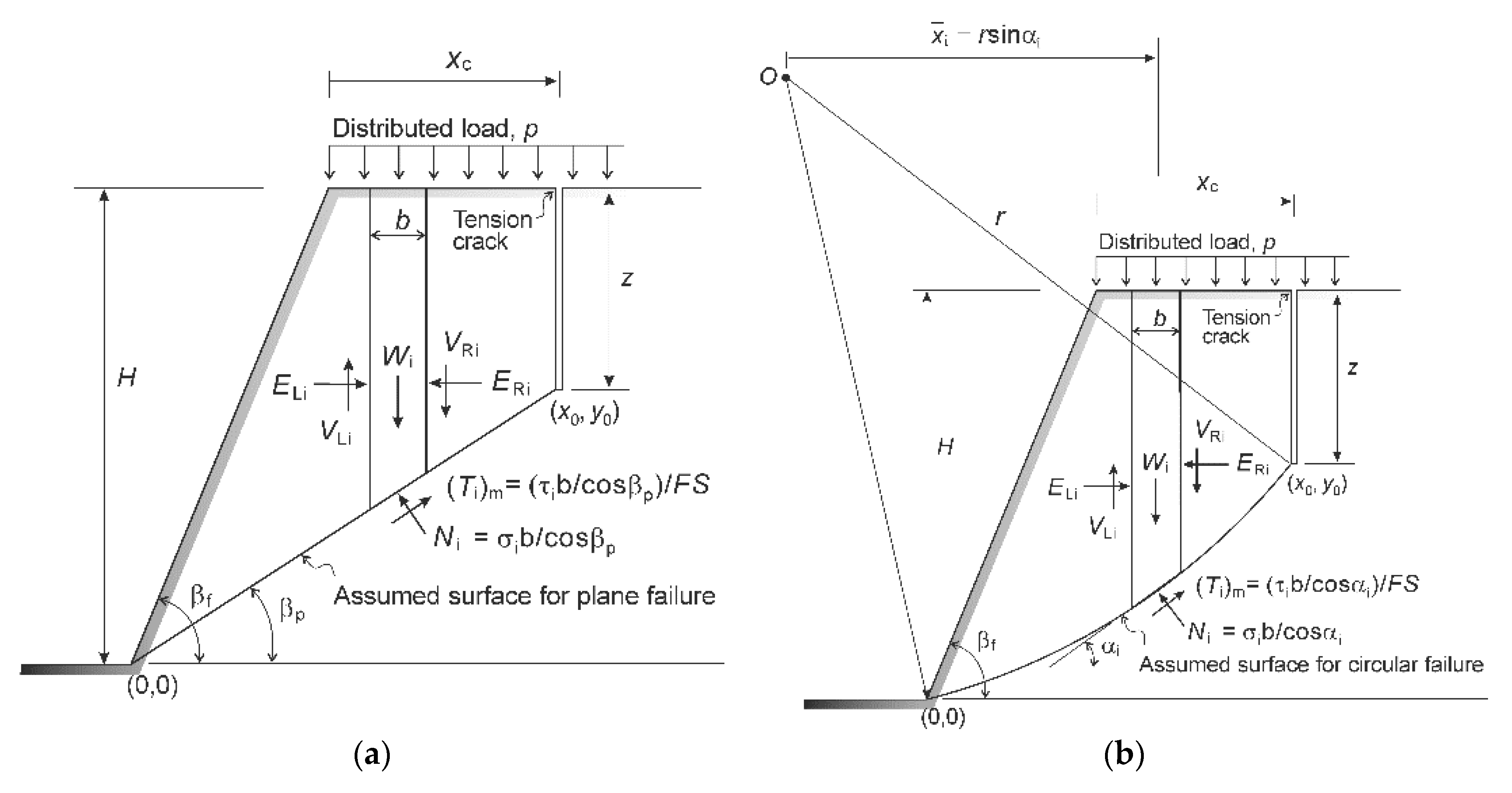
4.1. Geometry of Rock Slope Models

Figure 7a,b show the geometric configuration together with the assumed failure mechanisms. The slope geometry is defined by its height H and the face angle ${\beta }_f$. In both models analyzed here, it is assumed that a vertical tension crack of depth z is embedded at a distance $x_c$ from the crest and the distributed load p acts on the horizontal upper surface of the slope. Two distinct failure modes are considered involving a planar surface with the inclination angle ${\beta }_p$ and a circular failure surface, both passing through the toe of the slope and the tip of the crack. Given that the coordinates of the crack tip are $\left(x_0,y_0\right)$, the minimum radius of the circular surface is

$$r_{\min }=\frac{x_0^2+y_0^2}{2x_0}$$

(31)

The analysis employs the method of slices. For a circular slip surface, ${\alpha }_i$ represents the inclination of the base segment of the ith slice, whereas the corresponding distance from its mid-point to the center of rotation is $\overline{x_i}=r\sin {\alpha }_i$.

Figure 7. Geometry of slope showing forces of interaction acting on a typical slice: (a) model for plane failure; (b) model for circular failure.

Figure 7. Geometry of slope showing forces of interaction acting on a typical slice: (a) model for plane failure; (b) model for circular failure.

4.2. Modified Bishop Approach for the Assessment of Safety Factor

The analysis presented here is conducted using a modified version of Bishop’s simplified method. This approach is conceptually different from the original one (e.g., [33]). It invokes the classical framework of limit equilibrium analysis whereby an a priori assumption is made regarding the geometry of the failure surface along which the failure criterion is satisfied, and the safety factor is assessed by considering the global conditions of equilibrium. This is unlike the original Bishop approach in which the assessment of global stability is based on the notion of a local safety factor defined to estimate the current/mobilized shear stress. It is noted that the formulation of the simplified Bishop method, which incorporates a nonlinear relation for the safety factor requiring an iterative solver, raises some concerns. First of all, the assessment of the value of mobilized shear stress based on the failure condition that is satisfied only at the onset of failure may be questioned. In fact, prior to failure, the shear stress cannot be perceived as a unique function of normal stress. In addition, there is no basis for assuming that the local safety factor is constant within the domain. Given those concerns, the modified approach proposed here is not only computationally more efficient but also appears to be more rigorous.

For a circular failure surface (Figure 7b), the global safety factor is defined as the ratio of the moment resisting sliding to the overturning moment, both taken about the center of rotation. For the entire sliding wedge considered as a free body, the overturning is triggered by the own weight and the external load p, while the resisting moment is due to the shear stress distribution along the failure surface. Thus, summing up the contribution from individual slices, the safety factor (FS) is defined as

$$FS=\frac{\sum {\tau }_i b\sec {\alpha }_i}{\sum \left(w_i+pb\right)\sin {\alpha }_i}$$

(32)

where $w_i$ is the weight of the slice and ${\tau }_i$ is the shear stress which, at the inception of the loss of stability, satisfies the local failure condition ${\tau }_i=\tau \left({\sigma }_i\right)$ as defined by Equation (29). It should be noted here that for all slices intercepting the slope there is $p=0$, as the distributed load acts only along the horizontal boundary.

The expression for the safety factor, viz. Equation (32), is now supplemented by considering the equilibrium of an individual slice. Referring again to Figure 7, $V_i$ and $E_i$ are the shear and normal forces of interaction between the slices. Neglecting now the variation in shear forces, i.e., taking $V_{Li}=V_{Ri}$ as commonly assumed in the Bishop simplified approach [25], and invoking the force equilibrium in the vertical direction, yields

$$W_i+pb-{\sigma }_i b-{\tau }_{i}b\tan {\alpha }_i=0$$

(33)

Again, since along the rapture surface the failure criterion is said to be satisfied, there is ${\tau }_i=\tau \left({\sigma }_i\right)$ as stipulated in Equation (29). Thus, given Equation (33), the value of ${\sigma }_i$ for each slice can be determined, which in turn defines the individual terms in the expression for the global safety factor (32).

It should be noted that in the original version of the simplified Bishop method, the equilibrium statement explicitly incorporates a local safety factor, i.e.,

$$W_i+pb-{\sigma }_i b-\frac{1}{FS}{\tau }_{i}b\tan {\alpha }_i=0$$

(34)

In this case, the problem becomes nonlinear and the simultaneous Equations (32) and (34) are solved in an iterative manner. Apparently, in case of a planar failure mode (Figure 7a), ${\alpha }_i$ in Equations (32)–(34) is replaced by a constant angle ${\beta }_p$.

For the circular failure mode, the factor of safety varies with the assumed radius r of the sliding block. In this case, the determination of FS represents a unimodal optimization problem for finding the critical radius that minimizes the factor of safety within the interval $r_{min}\le r<\infty$. Recall that the minimum radius ($r_{min}$) can be calculated by Equation (31). In this paper, the minimum FS was determined by employing the golden section search algorithm [34]. In the examples that follow, the proposed approach is named as the modified Bishop method, while the approach incorporating Equation (34) is referred to by its original name, i.e., the simplified Bishop method.

4.3. Comparison of Safety Factors Based on the Simplified and Modified Bishop Methods

The simulations have been carried out assuming $H=35 \mathrm{m}$ and ${\beta }_f=70°$, while the strength parameters were taken as ${\sigma }_{ci}=20 \mathrm{MPa}$, $m_i=10$, $D=0$. The unit weight of rock was assumed as $\gamma =26 \mathrm{kPa}/\mathrm{m}$. In the example given here, no distributed load was considered, i.e., $P=0$.

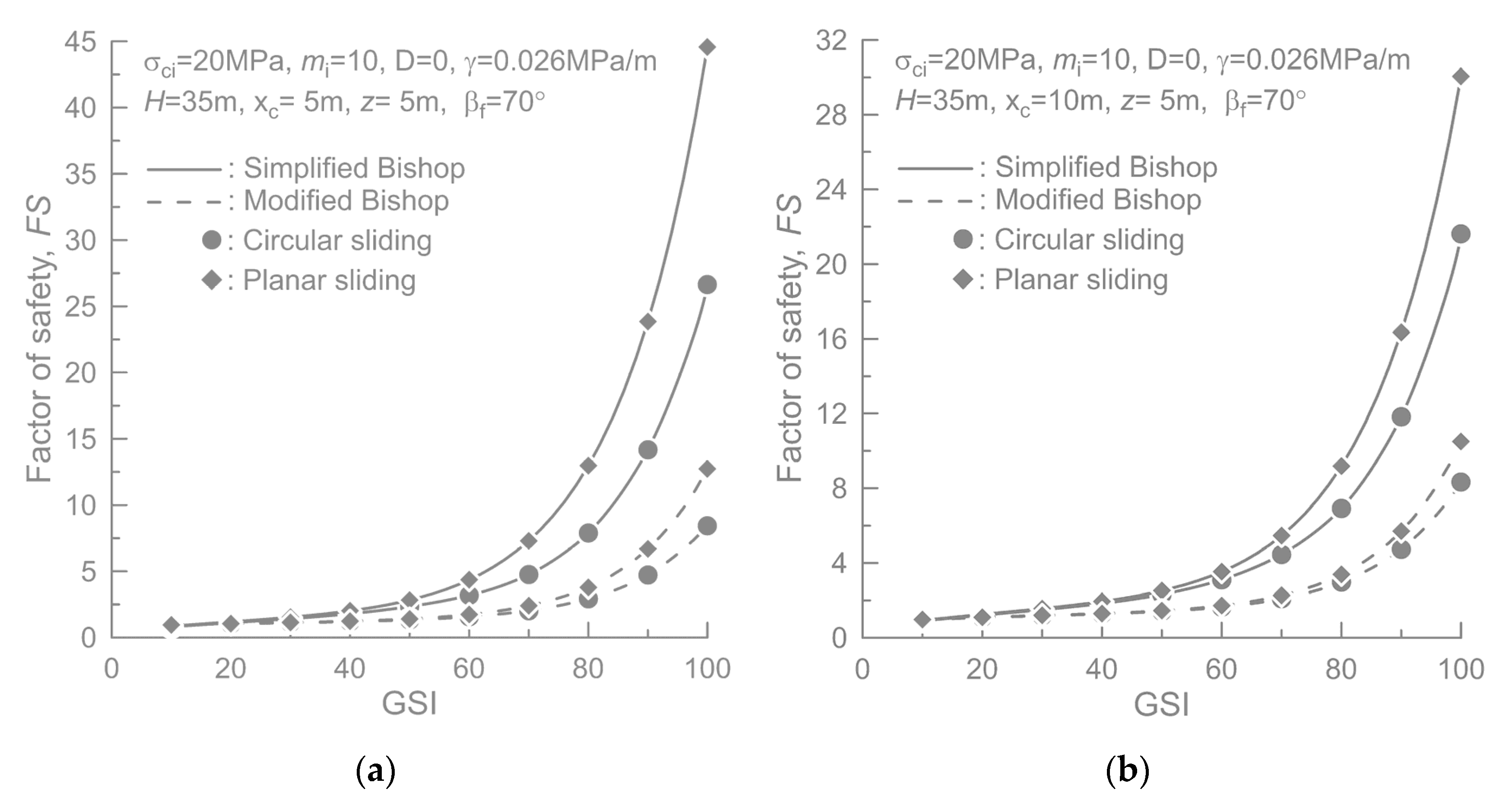
Figure 8 shows the variation in the safety factor as a function of GSI for the slope models having a 5 m deep tension crack. Two different horizontal positions of the crack, i.e., (a) $x_c=5 \mathrm{m}$, (b) $x_c=10 \mathrm{m}$, are considered. In the figure, the results obtained by assuming the plane and circular failure surfaces are presented together for the purpose of comparison. It is evident that the simplified Bishop method predicts larger FS than the modified approach. When $x_c=10 \mathrm{m}$ and GSI = 40, for example, the safety factors for circular failure surface are 1.84 with the simplified method and 1.27 with the modified approach, while the respective factors of safety for a plane failure surface are 1.94 and 1.30. However, as the GSI value decreases, the difference becomes smaller. This is because the global FSs from both methods approach unity as the rock mass quality becomes poorer. Here, it should be noted that both methodologies predict the same condition for the onset of the loss of stability, i.e., the case when $FS=1$. Another interesting feature is that, in the case of the modified method, there is little change in the safety factor when the GSI value is between 10 and 50. Thus, the modified method predicts a more conservative safety factor in a wide range of rock mass quality.

Figure 8 also reveals that the FS for the planar failure is larger than that for the circular failure, and the difference reduces again as the GSI value decreases. This trend can be attributed to the fact that the failure surface which yields the minimum FS becomes flatter as the rock mass properties degrade, cf. Figure 9. However, it should be kept in mind that these results correspond to an isotropic continuum and are different from the case of structurally controlled planar sliding commonly occurring in many rock slopes.

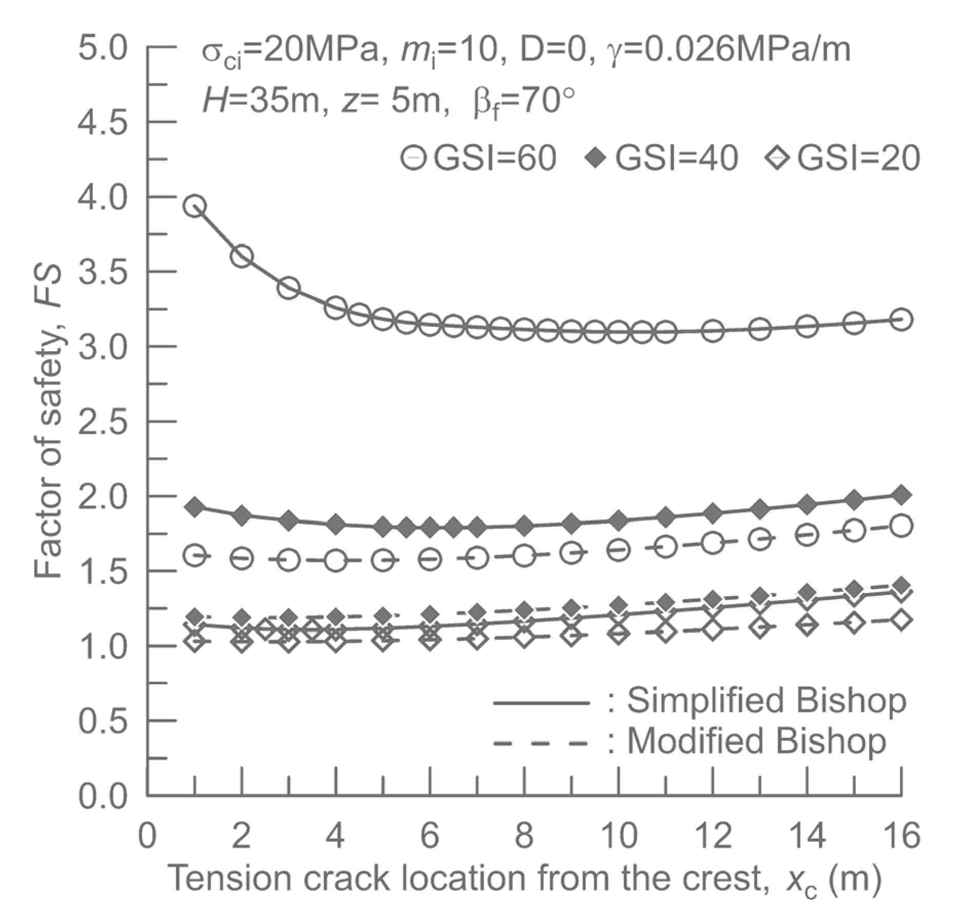
Finally, Figure 10 shows the variation in safety factor with the distance ($x_c$) defining the crack location. The trend is different for both methodologies. It is interesting to note that for large values of GSI, e.g., GSI = 60, the safety factor based on the simplified method decreases quite abruptly with increasing value of $x_c$ when the crack is near the slope. The latter is intuitively not correct as it implies that the cracks at locations closer to the crest result in a more stable configuration. Here, the results based on the modified method appear to be more consistent.

4.4. Assessment of the Critical Value of Surface Load

In this section, the critical value of distributed load p, which results in the loss of stability, was assessed for the same slope geometry as that shown in Figure 8. Since in this case the solution requires FS = 1, both methodologies yield the same results, while the modified Bishop method is simpler and computationally more efficient. The latter approach was implemented here in an iterative manner by adjusting the value of p until the safety factor became close to 1.

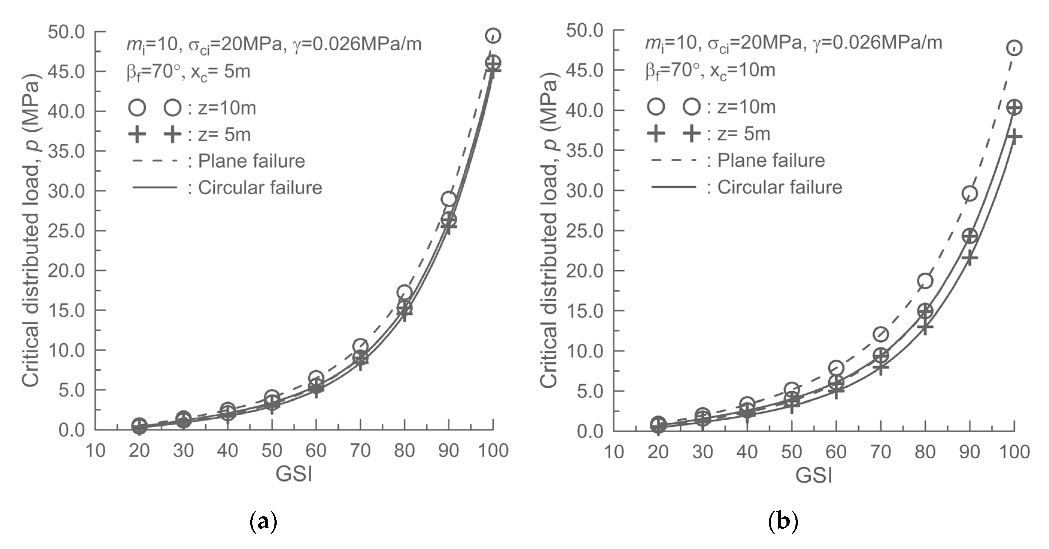
Figure 11 shows the predicted variation in critical load as a function of GSI for two different crack depths, i.e., z = 5 m and 10 m, and two crack locations, i.e., $x_c=5 \mathrm{m}$ and 10 m. It is seen that the critical load increases exponentially as the GSI value increases. It is also evident that the critical load for plane failure is larger than that for circular failure, which is consistent with the FS calculation results given in Figure 8. 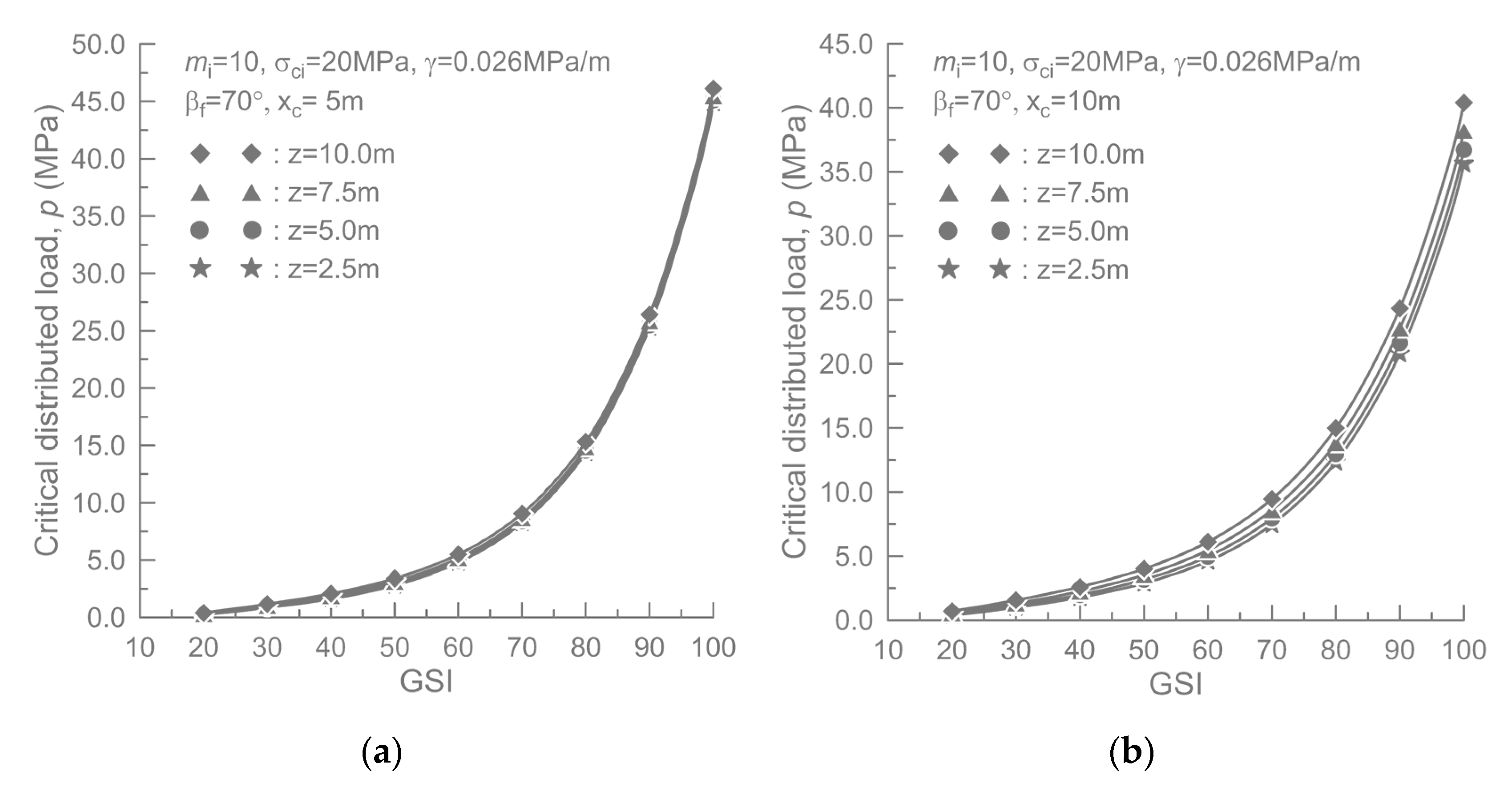Another observation, which stems from the result shown in Figure 11, is that the critical load increases with increasing crack depth. This may be due to the fact that, as the crack depth increases, the average inclination of the sliding surface decreases, and consequently it becomes more resistant to failure. To examine the effect of crack depth in more detail, the critical loads were calculated for four different depths by assuming a circular failure mode (Figure 12). In this case, it is apparent that the effect of crack depth is less significant when the crack is located close to the slope, but the influence increases as the position of the vertical crack moves further away from the slope.

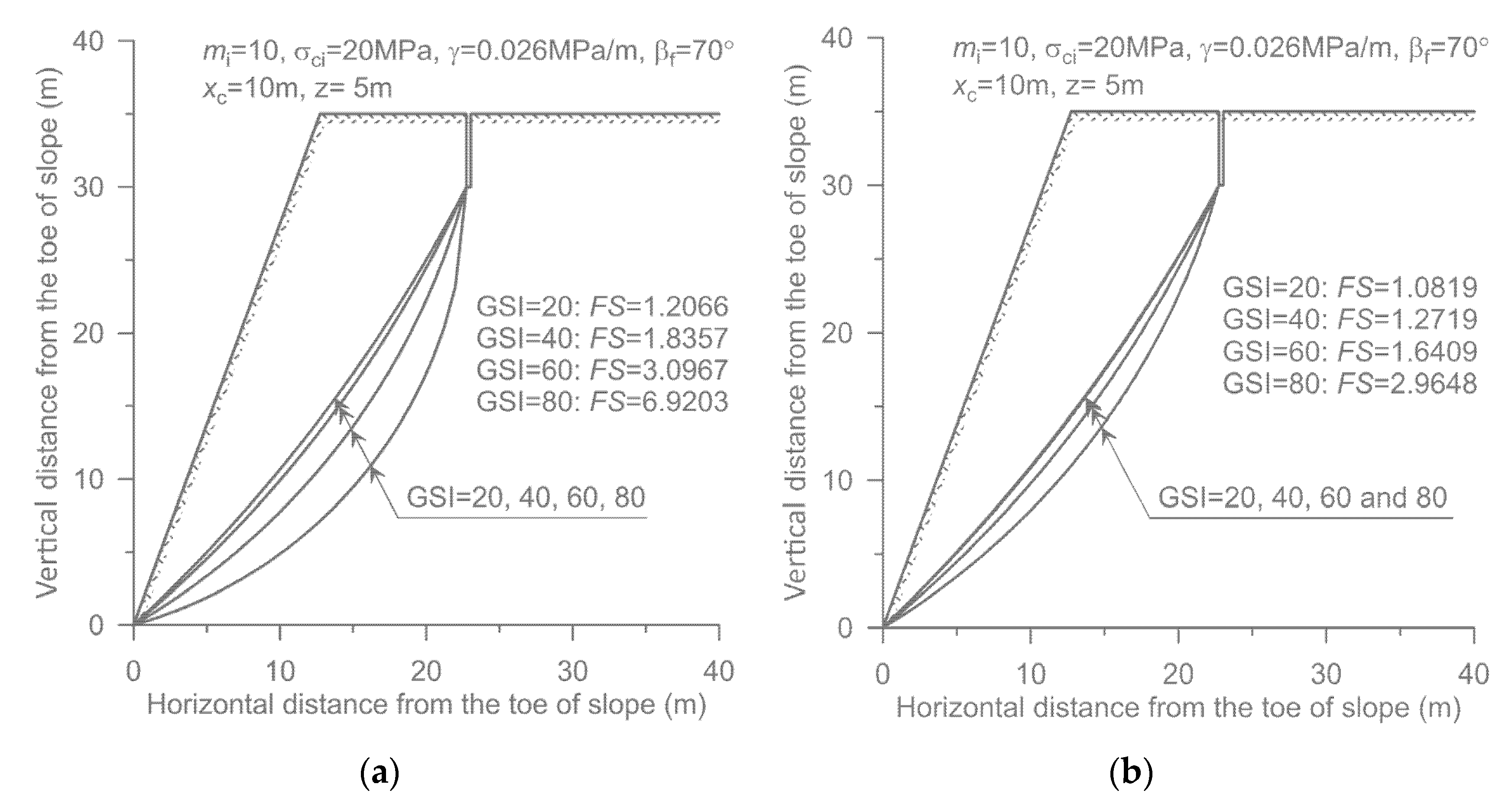
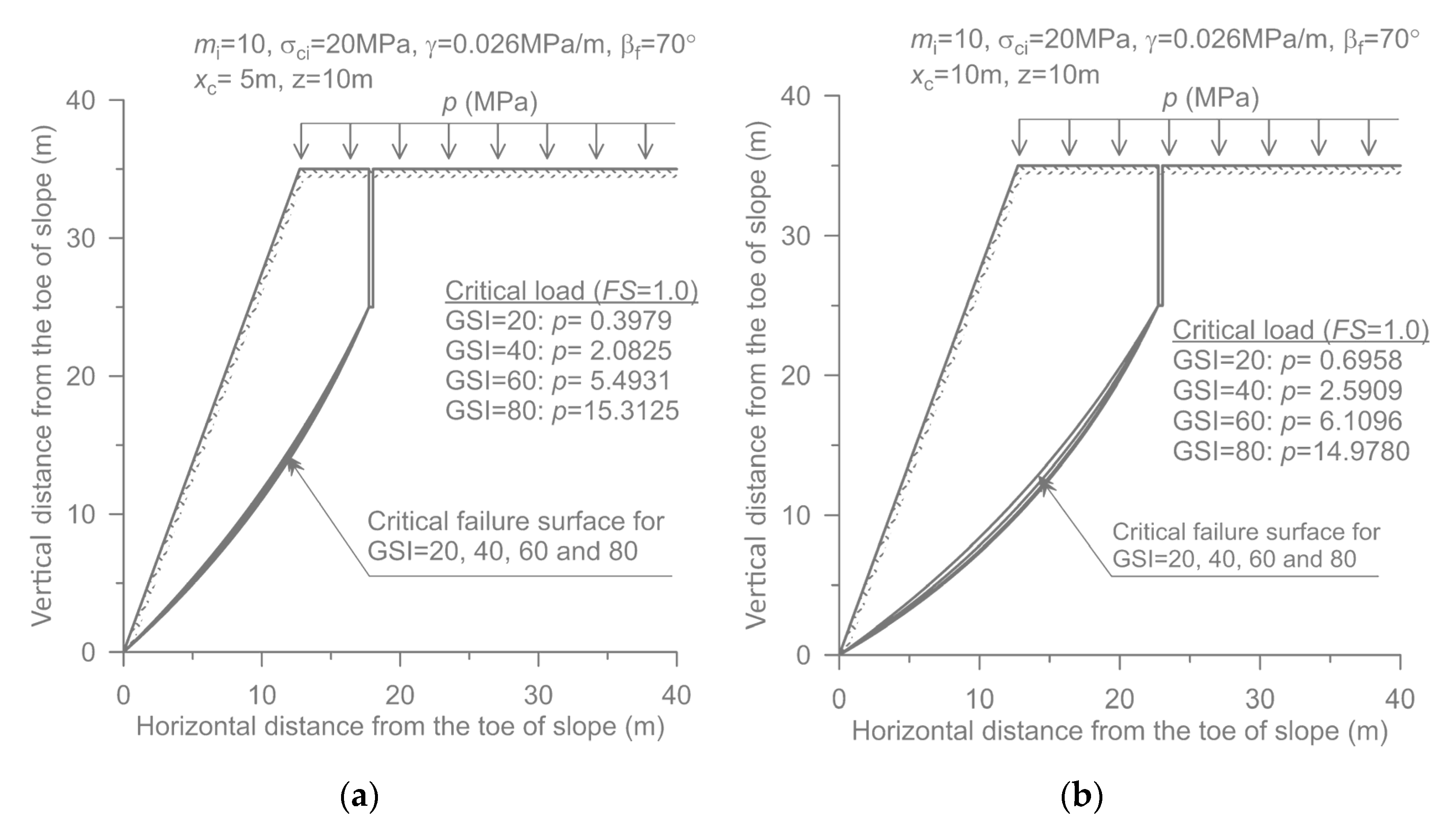
Finally, Figure 13 shows the geometry of critical failure surfaces associated with the loss of stability for GSI = 20, 40, 60 and 90. In this case, a 10 m deep vertical crack is assumed to be present at two locations, i.e., $x_c=5 \mathrm{m}$ and 10 m. The results indicate that, in this case, the influence of GSI value on the shape of the critical surface is not very significant.

5. Conclusions

The GHB criterion considers the nonlinearity of the rock mass strength and is applicable to a broad spectrum of rock masses, from weak to competent ones. However, a serious disadvantage of this criterion is that when $a\ne 0.5$, its shear strength–normal stress relationship, i.e., the Mohr envelope, is not available in the form of an explicit analytical expression. An alternative to overcome this difficulty is to define the Mohr envelope in an approximate analytical form. In this paper, a new approximate expression of Mohr envelope of the GHB criterion, which has much higher accuracy compared to other existing approaches, was proposed. 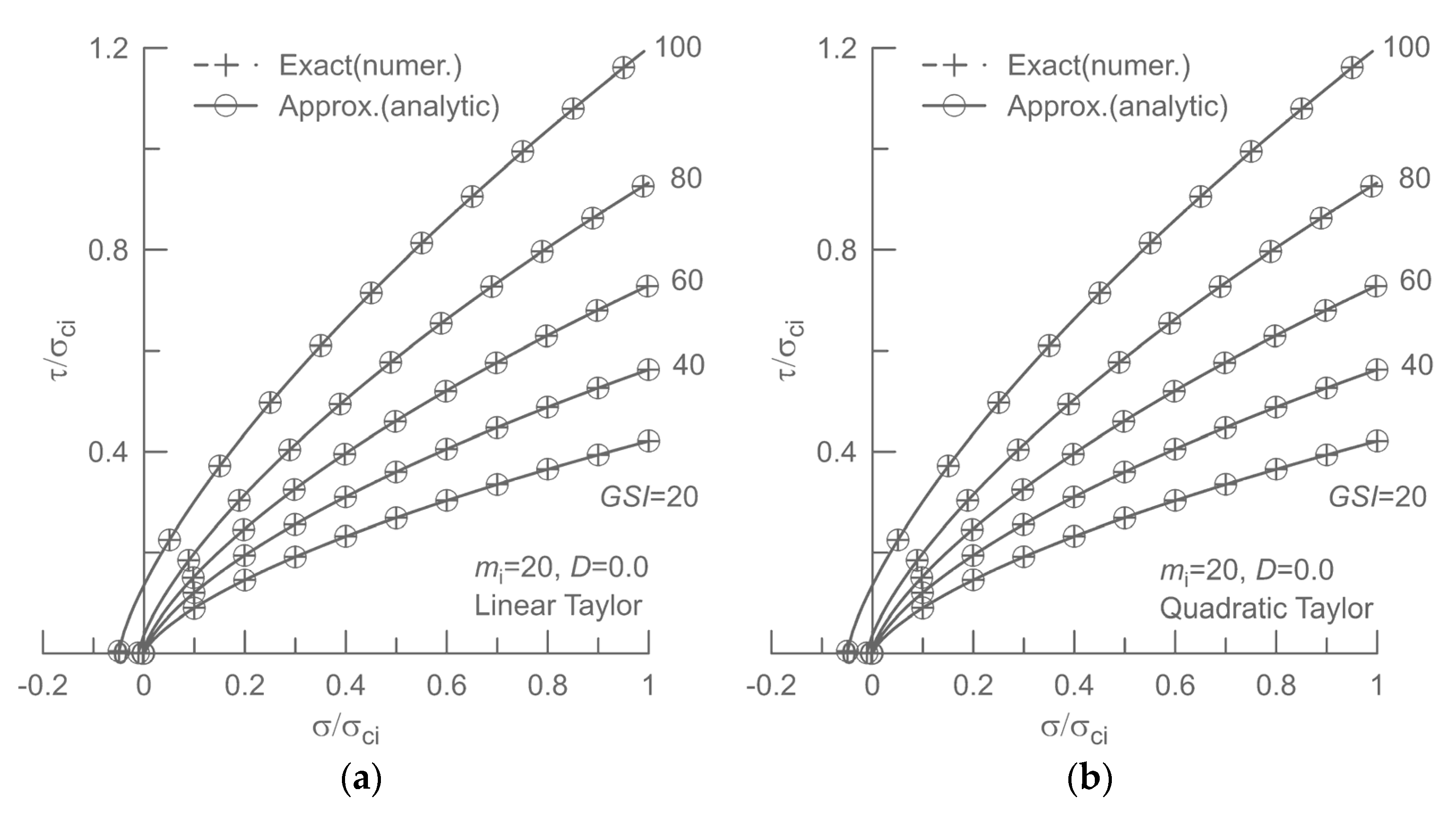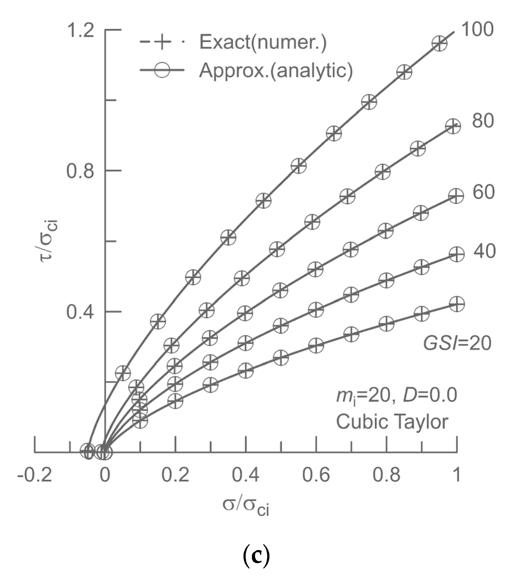The idea behind this formulation is to approximate Balmer’s equation [31], which defines the relationship between normal stress and minor principal stress at failure, by the Taylor polynomial equations of a finite degree that can be solved analytically in an explicit form.

At a first glance, the proposed formulation looks similar to that of Lee and Pietruszczak [15] in that it starts from the approximation of Balmer’s parametric equation which defines the relationship between the normal stress and the minor principal stress at failure. However, in the approach pursued here Balmer’s equation is approximated much more accurately by replacing the power function terms with the finite Taylor series centered at the exact root of Balmer’s equation for $a=0.5$. 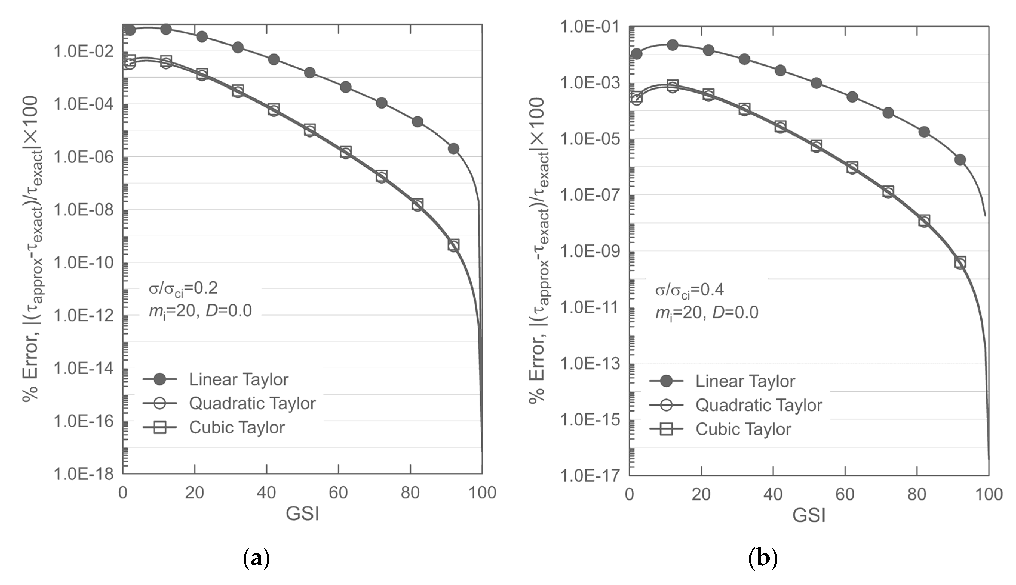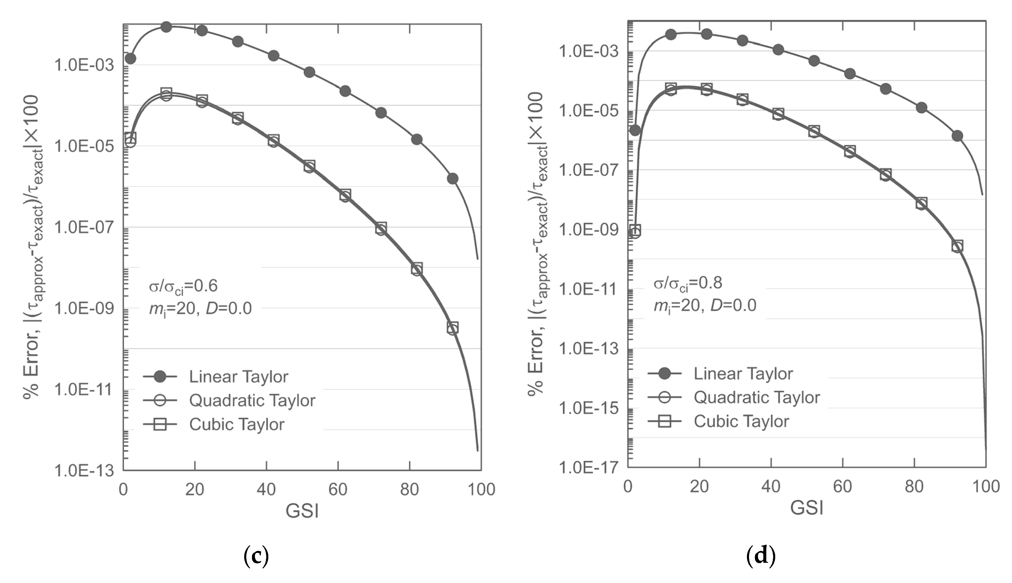The accuracy of the resulting approximate Mohr envelopes, incorporating the Taylor approximation of degree up to 3, was found to be superior to that of the recently published approximation of Lee and Pietruszczak [15]. Among the three cases considered, the one based on the quadratic Taylor approximation exhibited the best accuracy. Due to the mathematical constraints embedded in the Taylor approximation, as the GSI value approaches 100, the new three approximate Mohr envelopes come close to the exact Mohr envelope. Moreover, it can be shown that the accuracy of the proposed approach can be further improved if the solution is expressed in the form of a Coulomb equation employing the tangential friction angle of the approximate Mohr envelope, although in this case the resulting equations become algebraically more complicated. More importantly, since the proposed formulation of the Mohr envelope does not impose any restrictions on the range of ${\sigma }_3$, the high accuracy of the calculated shear strength can be retained in the whole range of normal stress. Therefore, it is expected that the newly proposed approximate Mohr envelope can find its applications when assessing the stability in the vicinity of a rock excavation surface where a relatively high stress gradient can occur.

As an example of application, the limit equilibrium analysis of a rock slope was carried out by incorporating the newly derived equation of the Mohr envelope based on the quadratic Taylor approximation. Two different approaches were considered, viz. the conventional simplified Bishop method and the modified Bishop method. In the proposed modified method, the factor of safety for slope failure is calculated in a global sense with the assumption that the current stress state satisfies the failure condition. The slope models employed in this study considered a vertical tension crack embedded in the upper horizontal surface, and the factors of safety have been calculated for varying crack position, crack depth and GSI value. In addition, the critical value of distributed load causing the loss of stability has been assessed for different cases. The results of the limit equilibrium analysis have shown that the factor of safety for plane failure is larger than that for circular failure. Furthermore, in a good quality rock mass the safety factor is more sensitive to the value of GSI than in a poor quality rock. Of the two equilibrium methods, the modified approach has resulted in a lower value of FS. However, the difference in the calculated FSs became smaller with the decrease in the value of GSI. The analysis has also shown that the critical magnitude of distributed load triggering the slope failure increases exponentially with the increase in GSI. However, for a given geometry of vertical crack, the GSI value did not significantly affect the shape of the critical circular surface. As the crack deepened, the critical load showed the tendency to increase, and this trend was more pronounced as the crack moved further away from the slope.

In conclusion, the illustrative examples given here demonstrated that the approximate equation of the Mohr envelope derived in this study can be conveniently used for stability analysis of slopes in the GHB rock mass, which is not feasible with the original form of the GHB criterion. The limit equilibrium analysis incorporated a modified version of the Bishop method. The latter is simpler and more rigorous than the original approach. Its implementation is quite straightforward, as it does not involve a nonlinear expression for the safety factor, and the estimates of stability are more conservative than those obtained using the conventional methodology.

Finally, it needs to be emphasized that the current study of slope stability is preliminary and serves mainly as an exploratory example. As mentioned earlier, the analysis employed a simple failure mechanism involving a circular surface passing through the toe of the slope and the tip of a pre-existing tension crack. Certainly, a proper verification of the proposed modified Bishop method requires a more in-depth study incorporating other failure mechanisms. Thus, even though the predicted basic trends are in line with an intuitive assessment, the quantitative verification is still required. In addition, some real case studies involving slope failures in rocks need to be examined to gain more confidence in the proposed methodology. Such studies are planned to be carried out in the future. In particular, the use of commercial software, such as FLAC, will be explored for comparison purposes. In addition, an upper bound limit analysis, incorporating the proposed approximation to the Mohr envelope, will also be pursued for a class of problems dealing with assessment of bearing capacity.

References

1. Hoek, E.; Carranza-Torres, C.T.; Corkum, B. Hoek–Brown failure criterion-2002 edition. In Proceedings of the 5th North American Rock Mechanics Symposium, Toronto, ON, Canada, 7–10 July 2002. [Google Scholar]
2. Marinos, P.; Hoek, E. GSI: A geologically friendly tool for rock mass strength estimation. In Proceedings of the GeoEng2000 at the International Conference on Geotechnical and Geological Engineering, Melbourne, Australia, 19–24 November 2000. [Google Scholar]
3. Marinos, V.; Marinos, P.; Hoek, E. The geological strength index: Applications and limitations. Bull. Eng. Geol. Environ. 2005, 64, 55–65. [Google Scholar] [CrossRef]
4. Wyllie, D.C.; Mah, C.W. Rock Slope Engineering, 4th ed.; Spon Press: London, UK, 2004. [Google Scholar]
5. Deng, D.P.; Li, L.; Wang, J.F.; Zhao, L.H. Limit equilibrium method for rock slope stability analysis by using the generalized Hoek-Brown criterion. Int. J. Rock Mech. Min. Sci. 2016, 89, 176–184. [Google Scholar]
6. Merifield, R.S.; Lyamin, A.V.; Sloan, S.W. Limit analysis solutions for the bearing capacity of rock masses using the generalized Hoek–Brown criterion. Int. J. Rock Mech. Min. Sci. 2006, 43, 920–937. [Google Scholar] [CrossRef]
7. Yang, X.L.; Zou, J.F. Stability factors for rock slopes subjected to pore water pressure based on the Hoek-Brown failure criterion. Int. J. Rock Mech. Min. Sci. 2006, 43, 1146–1152. [Google Scholar] [CrossRef]
8. Chen, W.F. Limit Analysis and Soil Plasticity; J. Ross Publishing: Fort Lauderdale, FL, USA, 2007. [Google Scholar]
9. Michalowski, R.L.; Park, D. Stability assessment of slopes governed by the Hoek-Brown strength criterion. Int. J. Rock Mech. Min. Sci. 2020, 127, 104217. [Google Scholar] [CrossRef]
10. Park, D.; Michalowski, R.L. Three-dimensional roof collapse analysis in circular tunnels in rock. Int. J. Rock Mech. Min. Sci. 2020, 128, 104275. [Google Scholar] [CrossRef]
11. Hoek, E. Strength of jointed rock masses, 23rd. Rankine Lecture. Geotechnique 1983, 23, 187–223. [Google Scholar] [CrossRef]
12. Ucar, R. Determination of shear failure envelope in rock masses. J. Geotech. Eng. Div. ASCE 1986, 112, 303–315. [Google Scholar] [CrossRef]
13. Londe, P. Discussion on “Determination of shear failure envelope in rock masses” by R. Ucar, J. Geotech. Eng. Div. ASCE 1988, 114, 374–376. [Google Scholar] [CrossRef]
14. Lee, Y.K.; Pietruszczak, S. Analytical representation of Mohr envelope approximating the generalized Hoek-Brown failure criterion. Int. J. Rock Mech. Min. Sci. 2017, 100, 90–99. [Google Scholar] [CrossRef]
15. Lee, Y.K.; Pietruszczak, S. Limit equilibrium analysis incorporating generalized Hoek-Brown failure criterion. Rock Mech. Rock Eng. 2021, 54, 4407–4418. [Google Scholar] [CrossRef]
16. Lee, Y.K. Approximate shear strength formula implied in the generalized Hoek-Brown failure criterion. Tunn. Undergr. Space 2018, 28, 426–441. [Google Scholar]
17. Gao, K.; Bozorgzadeh, N.; Harrison, P. The equivalence of three shear-normal stress forms of the Hoek-Brown criterion. Rock Mech. Rock Eng. 2019, 52, 3501–3507. [Google Scholar] [CrossRef]
18. Sofianos, A.I.; Nomikos, P.P. Equivalent Mohr–Coulomb and generalized Hoek–Brown strength parameters for supported axisymmetric tunnels in plastic or brittle rock. Int. J. Rock Mech. Min. Sci. 2006, 43, 638–704. [Google Scholar] [CrossRef]
19. Jimenez, R.; Serrano, A.; Olalla, C. Linearization of the Hoek and Brown rock failure criterion for tunneling in elasto-plastic rock masses. Int. J. Rock Mech. Min. Sci. 2008, 45, 1153–1163. [Google Scholar] [CrossRef]
20. Lee, Y.K. Analytical Formula for the Equivalent Mohr-Coulomb Strength Parameters Best-fitting the Generalized Hoek-Brown Criterion in an Arbitrary Range of Minor Principal Stress. Tunn. Undergr. Space 2019, 29, 172–183. [Google Scholar]
21. Renani, H.R.; Martin, C.D. Slope stability analysis using equivalent Mohr-Coulomb and Hoek-Brown criteria. Rock Mech. Rock Eng. 2020, 53, 13–21. [Google Scholar] [CrossRef]
22. Li, A.J.; Merifield, R.S.; Lyamin, A.V. Stability chars for rock slopes based on the Hoek-Brown failure criterion. Int. J. Rock Mech. Min. Sci. 2008, 45, 689–700. [Google Scholar] [CrossRef]
23. Wei, Y.; Fu, W.; Ye, F. Estimation of the equivalent Mohr-Coulomb parameters using Hoek-Brown criterion and its application in slope analysis. Eur. J. Environ. Civ. Eng. 2021, 25, 599–617. [Google Scholar] [CrossRef]
24. Fraldi, M.; Guarracino, F. Limit analysis of collapse mechanism in cavities and tunnels according to the Hoek-Brown failure criterion. Int. J. Rock Mech. Min. Sci. 2009, 46, 665–673. [Google Scholar] [CrossRef]
25. Yang, X.L.; Huang, F. Collapse mechanism of shallow tunnel based on nonlinear Hoek-Brown failure criterion. Tunn. Undergr. Space Technol. 2011, 26, 686–691. [Google Scholar] [CrossRef]
26. Suchowerska, A.M.; Merifield, R.S.; Carter, J.P.; Clausen, J. Prediction of underground cavity roof collapse using the Hoek-Brown failure criterion. Comput. Geotech. 2012, 44, 93–103. [Google Scholar] [CrossRef]
27. Kumar, P. Shear failure envelope of Hoek-Brown criterion for rockmass. Tunn. Undergr. Space Technol. 1998, 13, 453–458. [Google Scholar] [CrossRef]
28. Yang, X.L.; Yin, J.H. Linear Mohr-Coulomb strength parameters from the non-linear Hoek-Brown rock masses. Int. J. Non-Linear Mech. 2006, 41, 1000–1005. [Google Scholar] [CrossRef]
29. Yang, X.L.; Yin, J.H. Upper bound solution for ultimate bearing capacity with a modified Hoek-Brown failure criterion. Int. J. Rock Mech. Min. Sci. 2005, 42, 550–560. [Google Scholar] [CrossRef]
30. Rojat, F.; Labiouse, V.; Mestat, P. Improved analytical solutions for the response of underground excavations in rock mass satisfying the generalized Hoek-Brown failure criterion. Int. J. Rock Mech. Min. Sci. 2015, 79, 193–204. [Google Scholar] [CrossRef]
31. Balmer, G. A general analytical solution for Mohr’s envelope. Proc. ASTM 1952, 52, 1260–1271. [Google Scholar]
32. Press, W.H.; Teukolsky, S.A.; Vetterling, W.T.; Flannery, B.P. Numerical Recipes in Fortran, 2nd ed.; William H. Press: New York, NY, USA, 1992. [Google Scholar]
33. Das, B.M. Principles of Geotechnical Engineering, 4th ed.; PWS Publishing Company: Boston, MA, USA, 1997. [Google Scholar]
34. Chapra, S.C.; Canale, R.P. Numerical Methods for Engineers, 5th ed.; McGraw-Hill: New York, NY, USA, 2005. [Google Scholar]
Figure 1. Generalized Hoek–Brown criterion in the transformed nondimensional stress space.
Sustainability 14 12113 g001
Figure 2. Normalized Mohr envelope and Mohr circle of the generalized Hoek–Brown criterion.
Sustainability 14 12113 g002
Figure 3. Comparison of the proposed approximate Mohr envelopes with those obtained from the numerical (exact) solution: the approximate Mohr envelopes are calculated by using the proposed analytical shear strength formulas (Mohr envelopes) incorporating the approximate solutions for N 3 corresponding to (a) the linear, (b) quadratic and (c) cubic Taylor polynomial approximations of the Balmer’s equation.
Sustainability 14 12113 g003aSustainability 14 12113 g003b
Figure 4. Comparison of the approximate Mohr envelopes from Lee and Pietruszczak’s formula [15] with the numerical (exact) solution for the same rock mass conditions as in Figure 3.
Sustainability 14 12113 g004
Figure 5. Percentage errors incurred in the shear strength predictions using the newly formulated approximate Mohr envelopes and Lee and Pietruszcak’s formula [15] for rock masses with GSI values of (a) 20, (b) 40, (c) 60 and (d) 80.
Sustainability 14 12113 g005
Figure 6. Effect of GSI value on the percentage errors of shear strength prediction based on newly formulated approximate Mohr envelopes; (a) σ / σ c i = 0.2, (b) 0.4, (c) 0.6 and (d) 0.8.
Sustainability 14 12113 g006aSustainability 14 12113 g006b
Figure 8. Factors of safety versus the value of GSI for a slope with embedded vertical tension crack of depth 5 m located at (a) x c = 5 m and (b)   x c = 10 m.
Sustainability 14 12113 g008
Figure 9. The circular failure surfaces giving the minimum FS for four different GSI values; slope model with   x c = 10 m and z = 5 m: (a) simplified Bishop method; (b) modified Bishop method.
Sustainability 14 12113 g009
Figure 10. Variation in factor of safety with the location of 5 m deep tension crack for three different values of GSI: simplified vs. modified Bishop approach.
Sustainability 14 12113 g010
Figure 11. The critical value of distributed load versus GSI for two different crack depths, i.e., 5 m and 10 m; planar and circular failure modes: (a) xc = 5 m and (b) xc = 10 m.
Sustainability 14 12113 g011
Figure 12. The critical value of distributed load versus GSI for four different crack depths, i.e., 2.5 m, 5.0 m, 7.5 m and 10.0 m; circular failure mode: (a)   x c = 5 m; (b)   x c = 10 m.
Sustainability 14 12113 g012
Figure 13. The geometry of the critical circular failure surfaces for four different values of GSI, i.e., 20, 40, 60 and 80; slope model with a 10 m deep crack: (a)   x c = 5 m; (b)   x c = 10 m.
Sustainability 14 12113 g013
Publisher’s Note: MDPI stays neutral with regard to jurisdictional claims in published maps and institutional affiliations.