Soil Liquefaction Prediction Based on Bayesian Optimization and Support Vector Machines

Abstract

Liquefaction has been responsible for several earthquake-related hazards in the past. An earthquake may cause liquefaction in saturated granular soils, which might lead to massive consequences. The ability to accurately anticipate soil liquefaction potential is thus critical, particularly in the context of civil engineering project planning. Support vector machines (SVMs) and Bayesian optimization (BO), a well-known optimization method, were used in this work to accurately forecast soil liquefaction potential. Before the development of the BOSVM model, an evolutionary random forest (ERF) model was used for input selection. From among the nine candidate inputs, the ERF selected six, including water table, effective vertical stress, peak acceleration at the ground surface, measured CPT tip resistance, cyclic stress ratio (CSR), and mean grain size, as the most important ones to predict the soil liquefaction. After the BOSVM model was developed using the six selected inputs, the performance of this model was evaluated using renowned performance criteria, including accuracy (%), receiver operating characteristic (ROC) curve, and area under the ROC curve (AUC). In addition, the performance of this model was compared with a standard SVM model and other machine learning models. The results of the BOSVM model showed that this model outperformed other models. The BOSVM model achieved an accuracy of 96.4% and 95.8% and an AUC of 0.93 and 0.98 for the training and testing phases, respectively. Our research suggests that BOSVM is a viable alternative to conventional soil liquefaction prediction methods. In addition, the findings of this research show that the BO method is successful in training the SVM model.

1. Introduction

Solid-to-liquid transitions in granular materials are known as liquefaction, and may be caused by a growth in pore water pressure [1,2]. Seismic liquefaction of saturated soils, which occurs as a result of earthquakes, is one of geotechnical engineers’ most pressing problems. This is because the lateral expansion of soil mass might represent a significant hazard to civil engineering works in the area if it occurs [1,2,3]. As an example, after the Wenchuan earthquake of M 8.0 which struck China in 2008, both surface buildings and subsurface utilities were damaged by liquefaction [1,2,4]. Consequently, estimating the soil liquefaction potential is a significant issue, and must be considered when building civil engineering structures [5,6,7,8,9,10]. Soil liquefaction potential may be measured in a variety of ways, as described in the scientific literature (e.g., [11,12,13]). Since in situ observations can only be made in regions where testing may be done on site, most approaches rely on separating non-liquefaction sections from liquefaction components (e.g., the shear wave velocity (Vs) technique and flat dilatometer tests (DMTs)) [2,14]. Due to the great uncertainty in both soil properties and earthquake scenarios, it is difficult to find a single effective empirical formula for regression analysis. This is why scientists are working to develop scientific predictive methods that are simpler, more intuitive, and more accurate than the typical empirical models that were previously used to analyze soil liquefaction.

Liquefaction potential may be accurately predicted using artificial neural networks (ANN)-based models, the most extensively used of all (e.g., [15,16,17,18,19]). In fact, ANNs have been shown to be more efficient than statistical approaches, but they also display several shortcomings, such as slow convergence speed, over-fitting, falling into local minima, poor generalization, and so forth. Using post-liquefaction cone penetration test (CPT) and standard penetration test (SPT) data, Muduli and Das [20,21] created the multi-gene genetic programming (MGGP) technique to assess the ability of the soil to be liquefied. It was discovered that a new instrument for assessing liquefaction could be marketed and supported efficiently. Particle swarm optimization (PSO) was used to improve a neuro-fuzzy GMDH model created by Javdanian et al. [22]. This model was shown to be acceptable and reliable in this area. PSO was also hybridized with a kernel extreme learning machine (KELM) to evaluate liquefaction potential [23]. To forecast the likelihood of the soil liquefaction, Hoang and Bui [24] used a least squares support vector machine (LSSVM) and a kernel Fisher discriminant analysis. Their findings demonstrated that the suggested model is both acceptable and reliable in this domain. Soil liquefaction was also predicted using the ensemble group method of data handling (EGMDH) [25]. The EGMDH model was shown to be more accurate than the standard GMDH model in forecasting soil liquefaction. Rahbarzare and Azadi [26] proposed an improved fuzzy support vector machine (FSVM) based on PSO and a genetic method. According to the researchers, FSVM performance was improved by using PSO and genetic algorithms (GAs). It seems that machine learning models are able to solve liquefaction potential problems with an acceptable level of accuracy. It is important to note that such models have been successfully applied in different areas of civil engineering, as reported by many scholars [27,28,29,30,31,32,33,34,35,36,37,38,39,40,41,42,43,44,45,46,47,48,49]. Some studies also employed Bayesian models to model the liquefaction triggers [50,51,52].

SVM models have been frequently utilized to forecast soil liquefaction. This method has been hybridized with different optimization techniques, including genetic algorithms (GAs), differential evolution (DE), grey wolf optimization (GWO), and kernel Fisher discriminant analysis (KFDA) [24,53]. However, to the best of our knowledge, no study to date has hybridized SVM with the Bayesian optimization (BO) technique, which is one of the most effective optimization techniques. Thus, in order to forecast soil liquefaction potential, this research develops a hybrid intelligence model (BOSVM). The remainder of the paper is organized as follows: Section 2 explains the mechanics of soil liquefaction. Section 3 goes on to describe the SVM and BO frameworks, as well as the datasets that were employed in this investigation. The results and discussion are described in Section 4. Finally, Section 5 gives a summary of this study.

2. Process of Soil Liquefaction

Saturated cohesionless soils liquefy when pore pressure rises, causing a loss in firmness that may lead to cracking and crumbling [1]. More specifically, Sladen et al. [54] describe the process of soils losing their shear resistance when subjected to cyclic, monotonic, or shock loadings; subsequently, the soil flows like a liquid until the shear stresses that operate on its mass are equal to or lower than its lowered resistance. In a broader sense, liquefaction is a transition from solidity to fluidity that happens when the pore pressure and the functional stresses are increased or decreased [1]. When soils are subjected to shearing forces, they have a propensity to shrink in volume, which can lead to the process known as liquefaction. After being sheared, saturated loose soil tends to compact into tighter particles that take up fewer pore spaces, analogous to the way that water is driven out of pores when trapped in them. Penetrating shear loads may cause pore water pressures to increase over time if the drainage system is blocked. When this occurs, stress is transferred from the soil mass to the pore water, reducing the soil’s shear resistance and its effective stress [1]. Liquidity occurs when the soil’s shear resistance is less than its static, driving shear stress, allowing the soil to undergo structural damage. True liquefaction occurs only when the flow of soil is greater than the undrained residual shear resistance of a contracting soil under a static shear stress, according to Castro’s most restrictive description [55]. It is worth remembering that both cyclic and monotonic shear stresses may lead to the liquefaction of cohesionless, loose soil.

3. Method

Soil liquefaction was predicted using a hybrid of the SVM model and the BO algorithm. Input selection, data splitting, model construction, and evaluation were all part of the procedure. A flowchart of this study is shown in Figure 1.

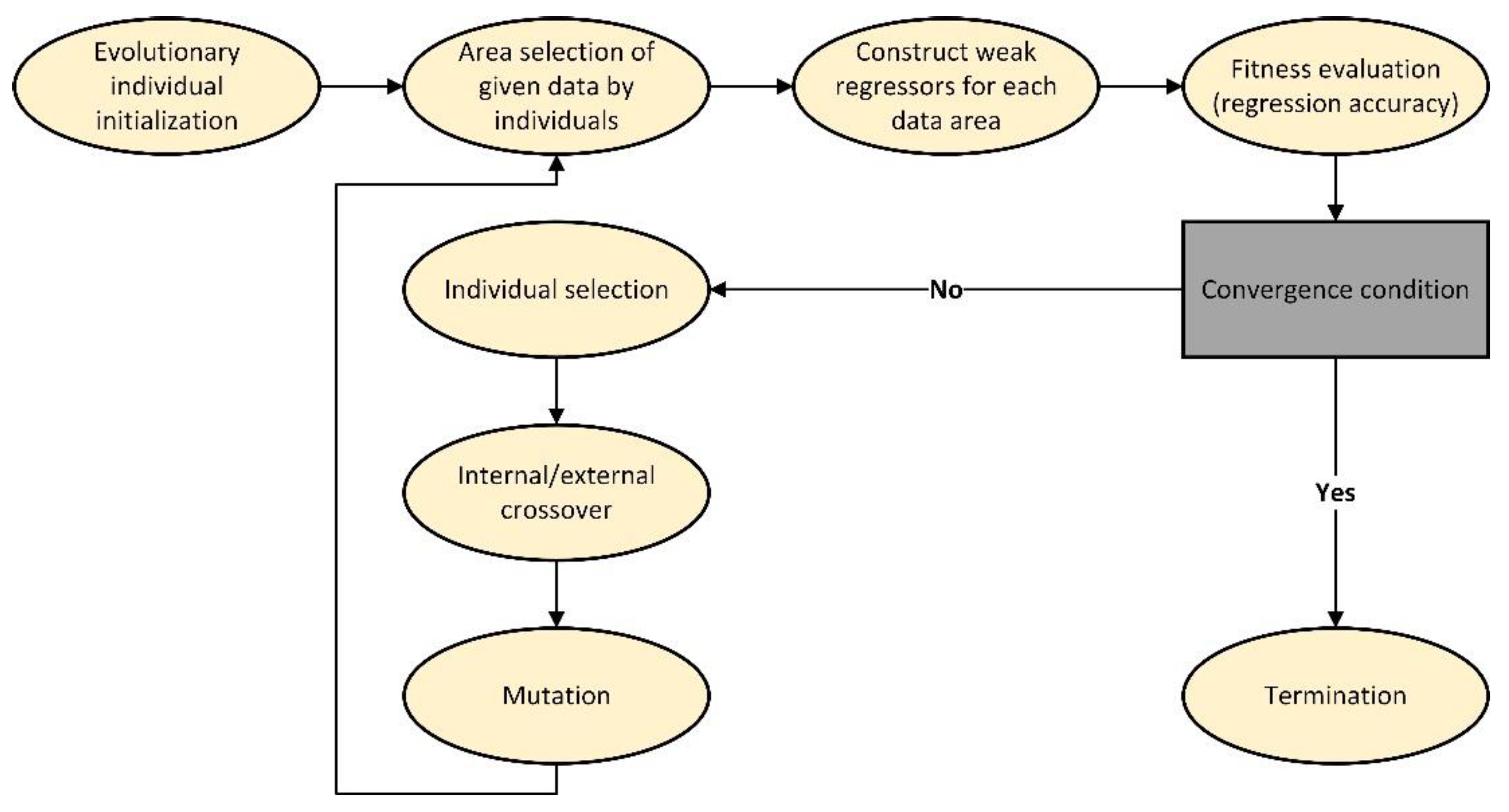
3.1. Evolutionary Random Forest (ERF)

Input selection is a critical step in the development of any ML model. Input selection refers to a process that identifies the most relevant inputs and removes irrelevant inputs from the dataset and modelling process. In this study, the evolutionary random forest (ERF) algorithm was employed. It is common practice to apply the random forest (RF) method and its ensemble theory when working with large datasets, selecting features for classification, and carrying out regression analyses. The RF method generates a variety of weak regressors based on decision trees (DTs) using randomly selected inputs or sample divisions from a training set. Each DT is created using data provided by the user, and generates a decision-making model. In other words, characteristics in the dataset are examined and disassembled in order to reach a satisfactory choice. Each model’s forecasted decision outcomes are obtained by the algorithm throughout the regression procedure. The mean of all the forecasts is used to reach the final forecast. Regardless of whether the overfitting issue is successfully mitigated, the RF’s arbitrary rule may impair learning capacity. As a result, the evolutionary computation that improves the subset sampling process [56,57] is expected to play a critical role in complementing the RF by enhancing the searchability of the complex objective function.

As can be seen in Figure 2, randomly generated rules at the start of the experiment determine data partitions and assign these subsets to each and every poor classifier/regressor. The regressors anticipate the value of the training data and collect the average forecasts to make a consensus. Regression accuracy results are used to gauge an individual’s fitness in the evolutionary process. To improve accuracy and genetic characteristics of the number of proposed individuals, repeated processes such as choosing, crossover, mutation, and evaluation are later applied. If the individuals converge, the algorithm stops the replicating phase and produces an optimum split of individuals as a model for regression. An ensemble regression based on a prior stage’s optimum individual is offered in this subsequent round of use of the trained model.

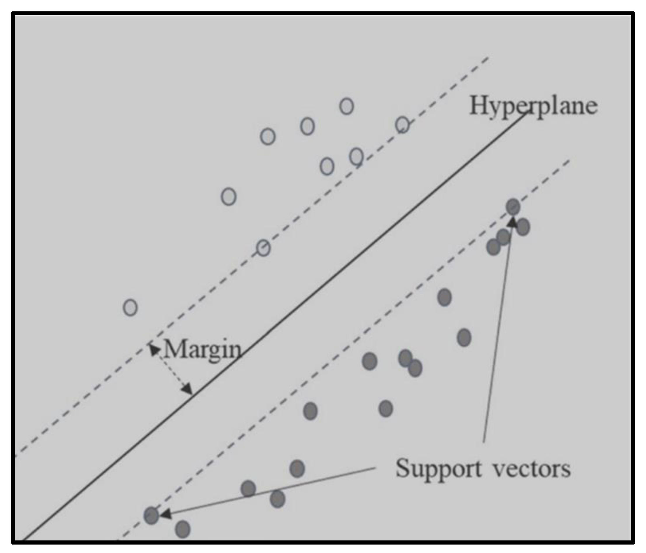
3.2. Support Vector Machines

SVM is a ML approach that incorporates various methodologies such as maximum interval hyperplane, relaxation variables, and kernel function. Statistical principles are behind this ML model. The classification difficulties associate with few samples, nonlinearity, and complexity may be solved with this method [58]. SVM has been progressively used in civil engineering as interdisciplinary integration has become more widespread. A nonlinear transformation is used to translate the input space samples into a high-dimensional characteristic space, and then an optimum classification plane is found that divides the samples linearly within the characteristic space as the next step [59,60]. The incidence of soil liquefaction functions well with the features of the approach to overcome binary classification issues in the study of soil liquefaction and its risk assessment (e.g., [61]).

Figure 3 depicts a schematic representation of the SVM concept. When a hyperplane is compared to a sample point, it is known as a margin. The classifier’s capacity to generalize improves with an increasing margin of error. As a result, finding the hyperplane that maximizes the margin (i.e., the ideal hyperplane) is the primary goal of the SVM. There are support vectors for every point on the hyperplane on either side of the margin, and the categorization border is decided only by the support vectors, not by additional data nor the quantity of data. Because of this, the optimization of the SVM’s hyperparameters is essential. Among the several hyperparameters used in SVM, kernel type, C, and gamma are among the most important. As previously stated, the kernel transforms the observed data into a feature space. By imposing a penalty for every incorrectly classified data sample, hyperparameter C manages the exchange between the decision boundary and precision. In various kernel types, gamma is a parameter linked to C. The influence of C is minimal when gamma is large. When gamma is modest, C has an effect on the model comparable to the effect it would have on a linear one.

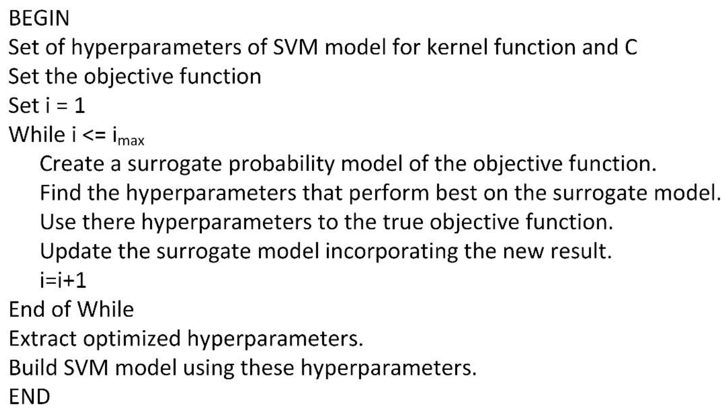
3.3. Bayesian Optimization Algorithm

The adjustment of learning parameters and model hyperparameters is an important part of the implementation of ML algorithms [62]. Model or training process qualities are defined by hyperparameters, which have a substantial impact on the model’s ultimate outcome [63]. Conventional ML algorithms use BO as a hyperparameter optimization (picking) strategy, as part of their overall design. The BO algorithm is extensively used in pioneering AI because of its evident benefits when compared with the particle swarm optimization algorithm, genetic algorithm, or other algorithms [63,64]. The Gaussian process and the Bayesian theorem are used to optimize parameters in this technique. A Bayesian ML approach and Gaussian process regression are used to generate a surrogate for the objective, and to quantify the ambiguity in that surrogate. To determine the sample position, an acquiring function can be expressed from this substitute. In Appendix A, the typical circumstances in which the BO algorithm encounters difficulties are explained. In addition, Figure 4 depicts a generic pseudocode of the BO.

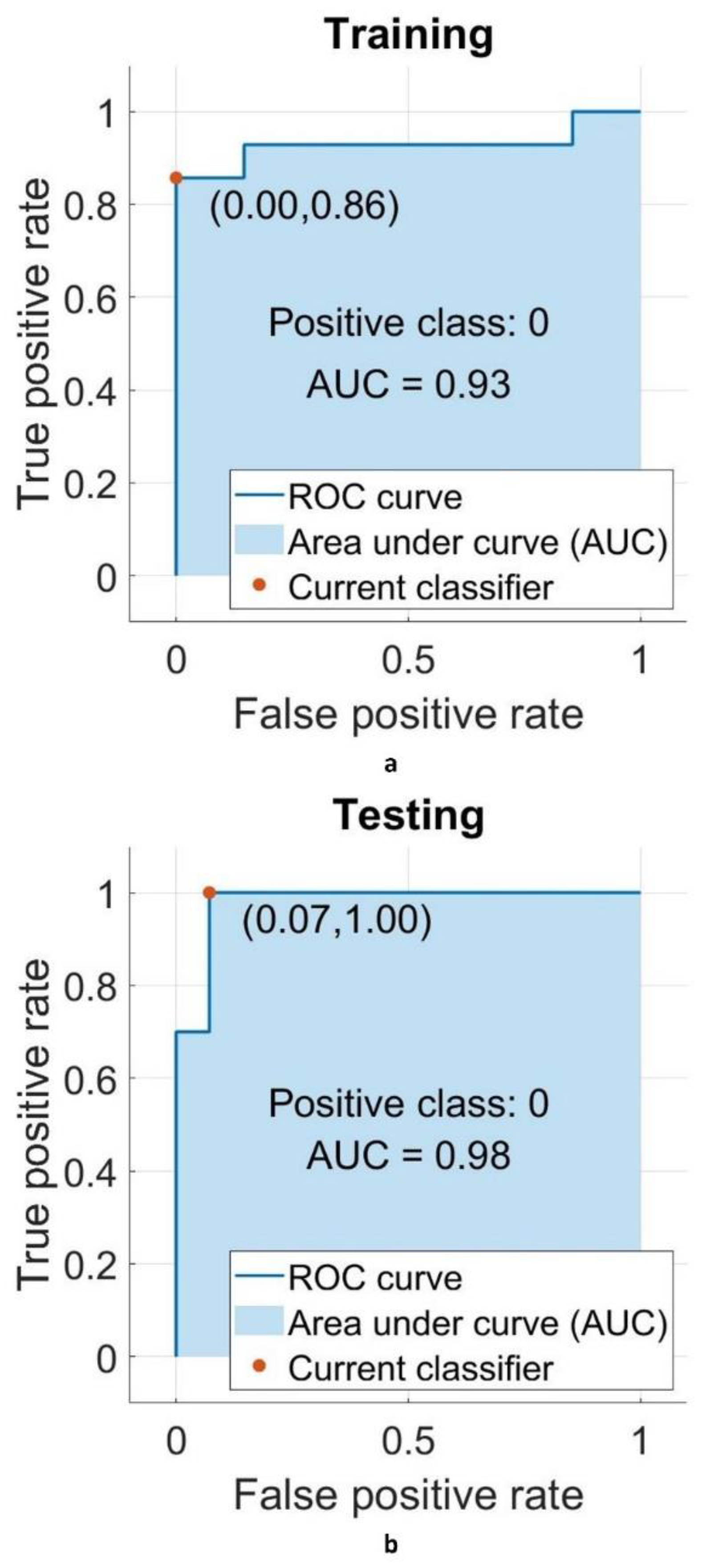
3.4. Performance Criteria

This study used several well-known performance criteria for classification. These criteria include the confusion matrix, accuracy (%), the receiver operating characteristic (ROC) curve, and the area under the ROC curve (AUC). The more accurate the model, the closer the curve is to the model’s top-left corner. AUC values fall within a range of 0 to 1. The greater the AUC, the more accurate the model.

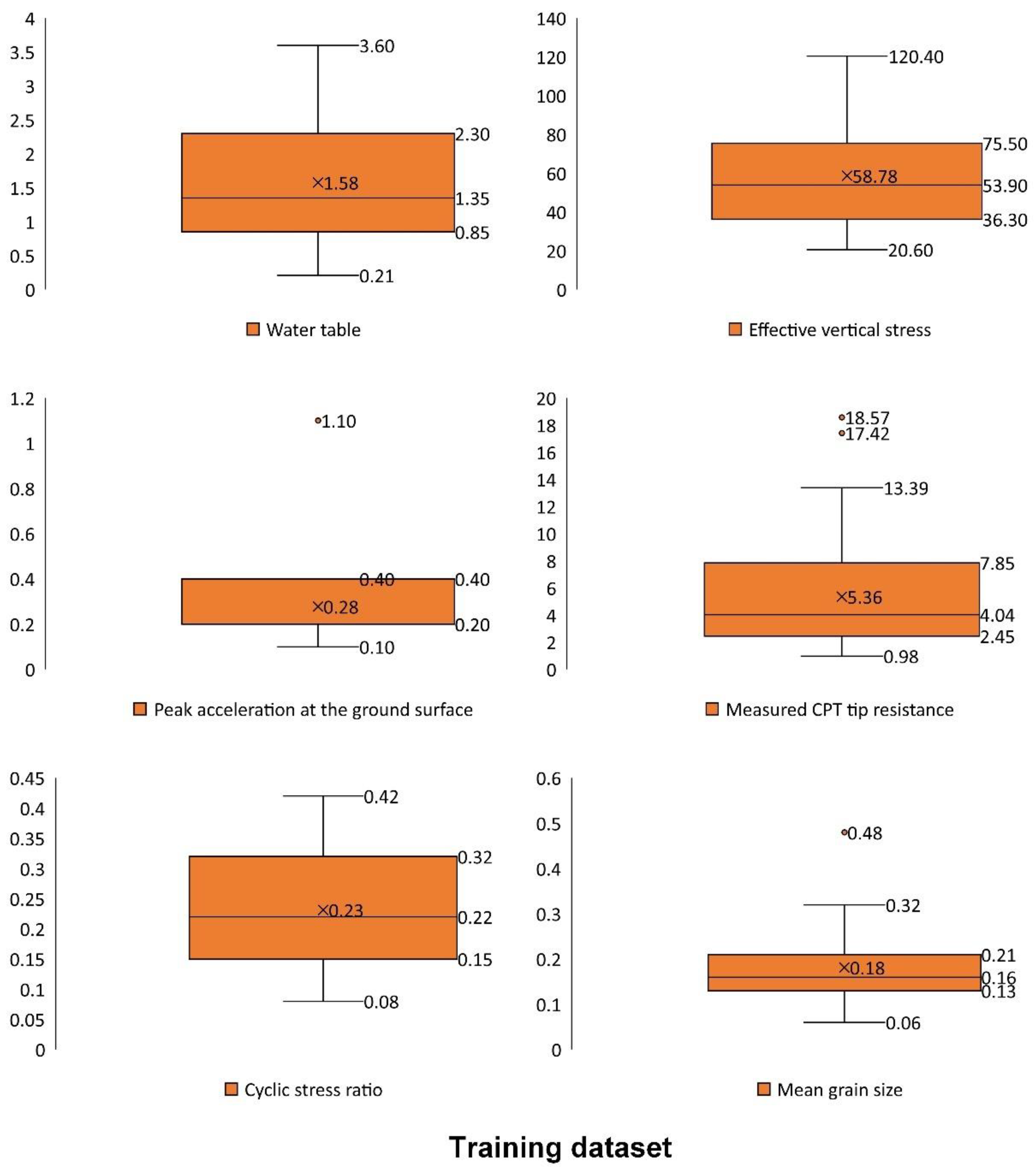
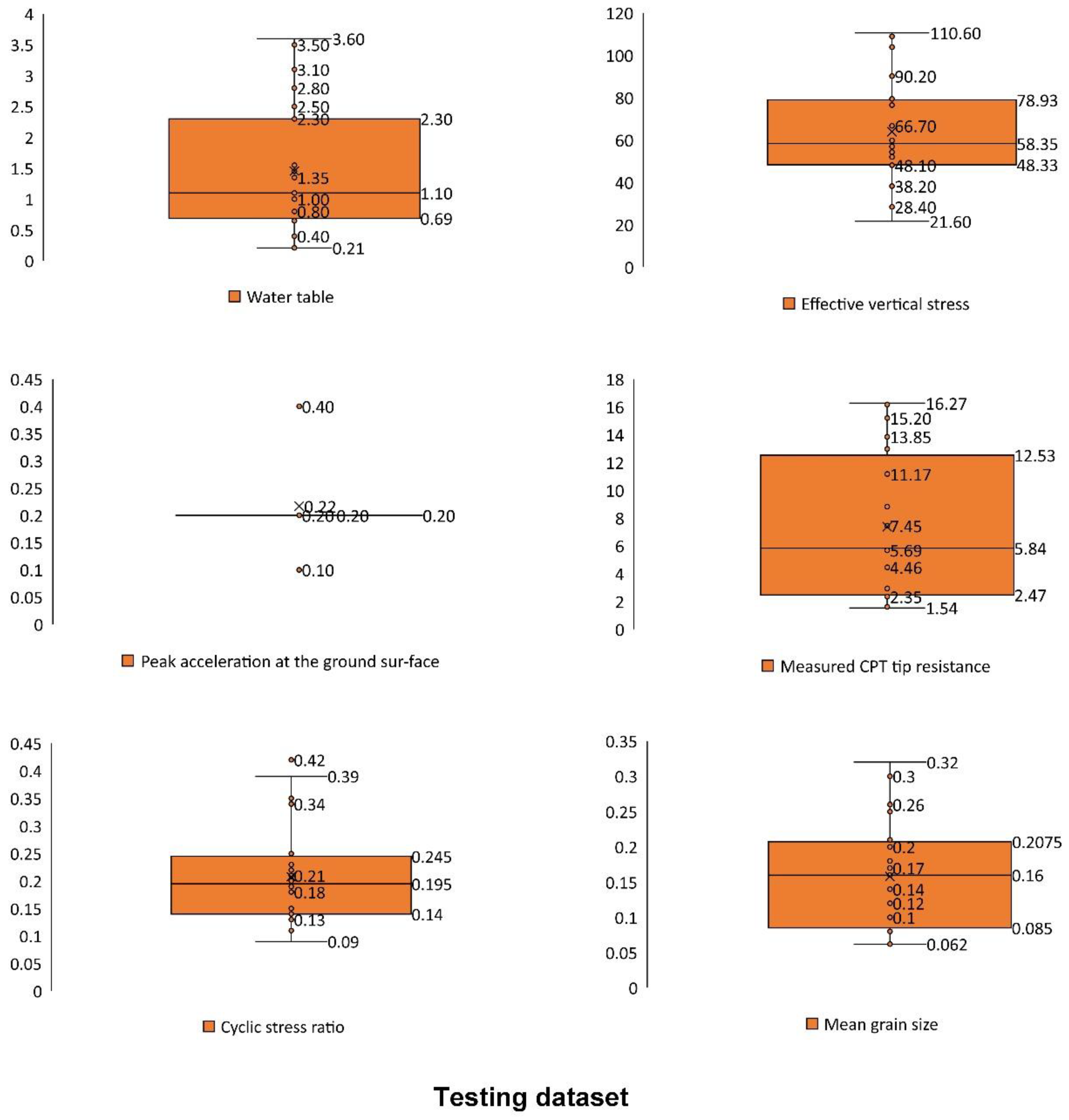
3.5. Data for Modeling

The Great Tangshan Earthquake, which occurred on 28 July 1976, was a major natural catastrophe in China. The number killed put the catastrophe at the top of the list of the most devastating earthquakes of the 20th century. Hebei’s industrial metropolis of Tangshan, home to almost a million people, was the epicenter of the earthquake. Initial estimates put the death toll at 655,000, but this has since been revised to between 240,000 and 255,000, with 164,000 people suffering from serious injuries [1]. In order to build the models described in this research, a database from prior studies was used [1]. The Tangshan Earthquake was the subject of this database [65]. Several entries were omitted from the final analysis, owing to incomplete or inaccurate data. Liquefaction potential was the sole parameter included in the model output. Variables used in this study are listed in

Table 1. Variables used in this study.

Variable	Symbol	Unit	Min	Max
Earthquake magnitude	M	-	7.8	7.8
Effective vertical stress	${\sigma }_{v0}^{\prime }$	kPa	20.6	120.4
Total vertical stress	${\sigma }_v$	kPa	16.7	244.2
Mean grain size	$D_{50}$	mm	0.06	0.48
Water table	$d_w$	m	0.21	3.6
Peak acceleration at the ground surface	$a_{max}$	g	0.1	1.1
Depth	$d_s$	m	0.9	13.1
Measured CPT tip resistance	$q_c$	MPa	0.98	18.57
CSR	$\frac{{\tau }_{av}}{{\sigma }_{v0}^{\prime }}$	-	0.08	0.42
Liquefaction observed *	-	-	0	1

* Target variable.

. A value of “1” indicates that liquefaction has occurred in each example, whereas “0” indicates that it has not. The overall cyclic shear stress caused by the earthquake is indicated by the term ${\tau }_{av}.$ Modeling included the utilization of 79 different sets of data. The data were split into training and test datasets, with a ratio of 70:30. To train the BOSVM model, this study used 5-fold cross-validation. The developed model was then tested using the test data.

4. Results and Discussion

4.1. Input Selection

Input selection is a critical phase in the machine learning modelling process [54,55,56,57,66,67,68,69], and is used to remove unnecessary variables while keeping those that are valuable. This study employed the evolutionary random forest (ERF) technique for input selection. The dataset used in this study consisted of nine candidate inputs, including $M, d_w, d_s, {\sigma }_v, {\sigma }_{v0}^{\prime }, a_{max}, q_c, CSR, \mathrm{and} D_{50}$. These nine parameters were selected because of their effects on the liquefaction from a geotechnical viewpoint; some of them were used in the previous related studies or suggested as the most influential factor in liquefaction occurrence [1,19,23,50,51]. Nonetheless, they have different levels of impact on liquefaction occurrence. It is necessary to keep intelligent models as simple as possible. This can be achieved by considering the most influential factors. To do this, the ERF selected six inputs, including $d_w, {\sigma }_{v0}^{\prime }, a_{max}, q_c, CSR, \mathrm{and} D_{50}$. Based on the ERF findings, a subset of these six inputs outperformed other input subsets on the dataset utilized in this research. These inputs were used to develop SVM and BOSVM models to predict soil liquefaction. It is important to mention that several parameters were used to develop the ERF model. The selection scheme was set as “tournament”, p initialize was set as 0.5, p mutation was set as −0.1, and p crossover was set as 0.5. The crossover type was uniform. The accuracy of this model was 92.50%.

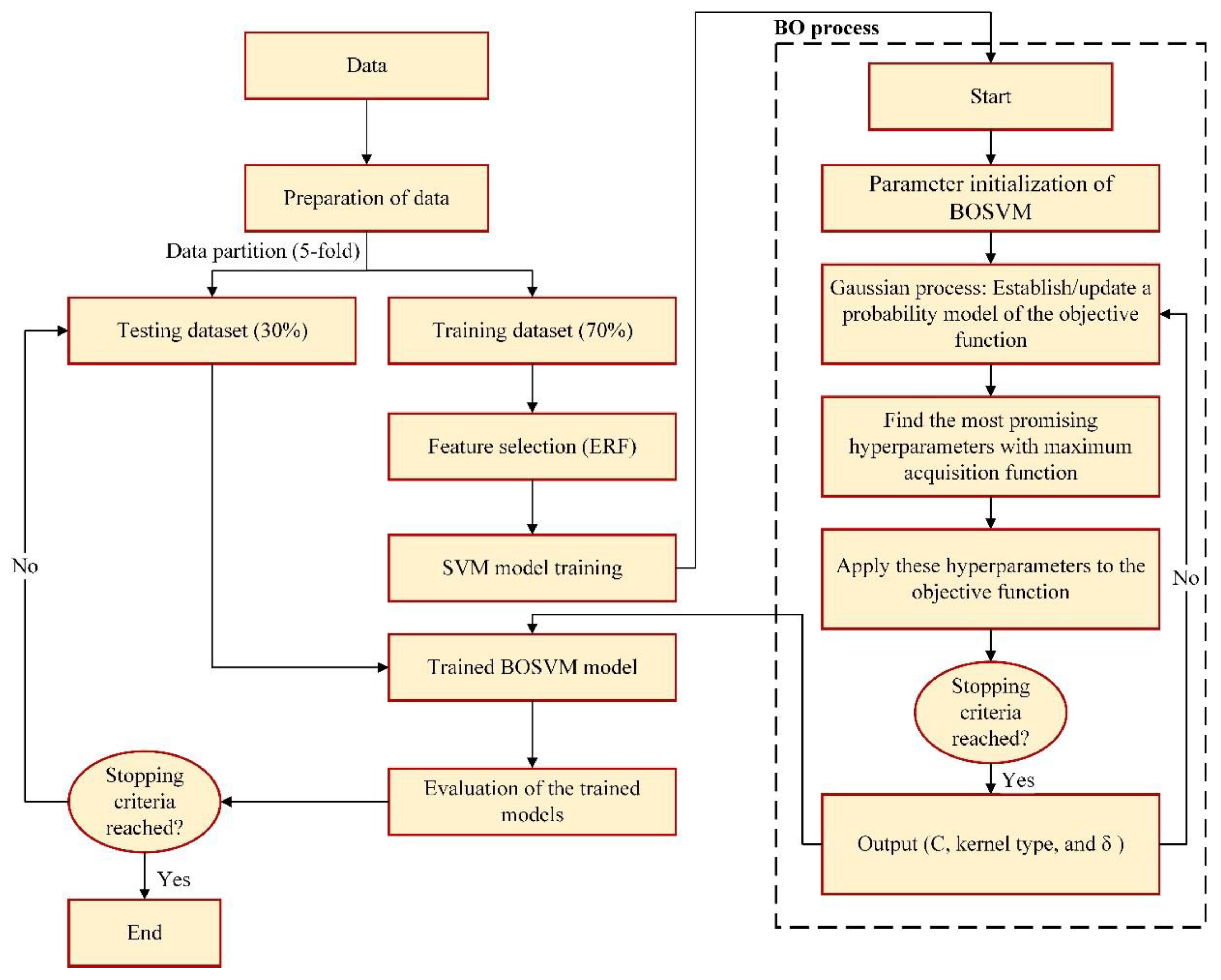
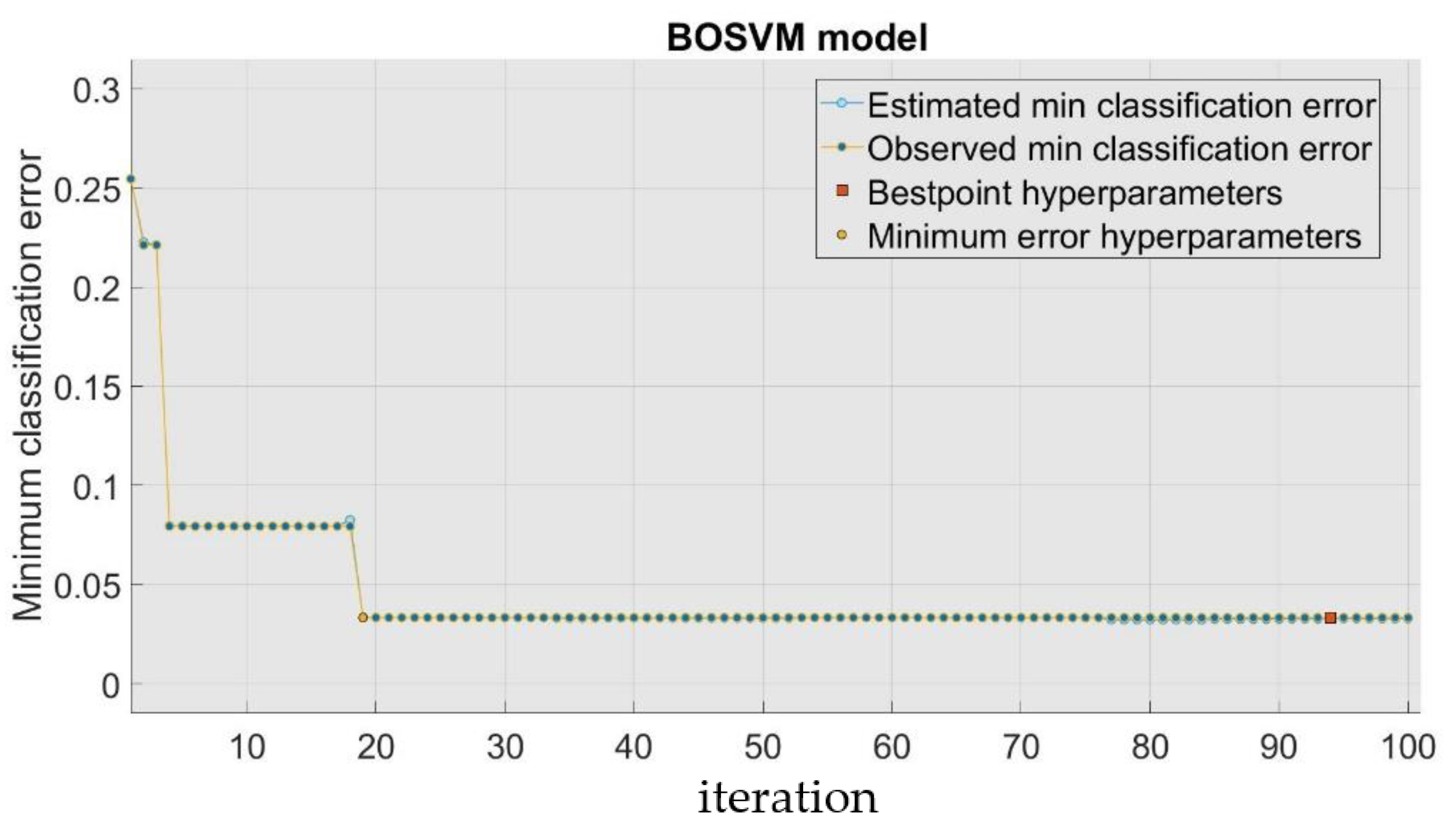
4.2. BOSVM Model Development

The hyperparameter optimization of the prediction model based on SVM was carried out using the Bayesian optimization (BO) approach in this work. Hyperparameters such as box constraint level and kernel scale were optimized using the BO technique for SVM models based on the hybrid model. These settings were configured from 0.001 to 1000. An overview of how the BO optimization method is used to optimize SVM parameters is provided below:

• Preparing the data: Using a suitable ratio, the data set is partitioned into training and testing sets (70:30). The distribution of inputs after the data split is shown in Figure 5 and Figure 6.
• Examination of fitness: The fitness function is computed and assessed before optimizing the target parameter value. The fitness function in this study is classification error.
• Adjusting the settings: hyperparameter optimization criteria may be adjusted according to the outcomes of each iteration, if desired.
• Stop checking for conditions: Optimization stops once the best parameters have been found.

SVM was used in conjunction with one optimization technique (i.e., BO) to create a hybrid intelligent model based on SVM that could better forecast soil liquefaction. As a result of the aforementioned optimization, several hyperparameter settings and model prediction results were produced.

One hundred iterations of the BOSVM model utilizing the fitness assessment of classification error were used to obtain the optimal SVM hyperparameters. As shown in Figure 7, convergence occurred in the BOSVM model before the maximum number of iterations had been completed. After 19 iterations using the BOSVM approach, the optimum SVM hyperparameters with the lowest classification error of 0.033 were found. This proves that the strategy is reasonably effective in identifying the optimum hyperparameters. The ability of BO to use all knowledge from prior runs in order to discover the next set of hyperparameters may explain this high rate of convergence [70,71].

As the kernel and regularization parameter (C) were optimized for BO, the linear kernel and a C value of 18.49 were the hyperparameters that best matched those values. Prior to modeling, these variables would be used as BOSVM hyperparameter values, whereas the standard SVM makes use of the default configuration. Both the SVM and BOSVM models were evaluated using the accuracy (%), confusion matrix, and ROC curve to verify and evaluate results. The ROC curve shows the predictive power of the models, while the confusion matrix shows the specifics of the model’s prediction capacity.

As stated in

Table 2. The confusion matrix of the models developed in this study.

Model		Train			Test
	Actual	Prediction			Prediction
		0	1	Accuracy (%)	0	1	Accuracy (%)
SVM	0	9	5	90.9	9	1	91.7
	1	0	41		1	13
BOSVM	0	12	2	96.4	10	0	95.8
	1	0	41		1	13

, the training accuracy of BOSVM is demonstrated to be 96.4%, which is almost 5.5% better than the SVM’s 90.9% training accuracy. Moreover, the SVM model’s test accuracy improved by 4.1% with the use of the BO algorithm. The BOSVM model’s training and testing accuracy are fairly close together, indicating the model’s stability in predicting soil liquefaction. Overall, soil liquefaction was better predicted with BOSVM than with SVM.

Figure 8 shows the ROC curve for both the training (Figure 8a) and testing (Figure 8b) phases. The ROC curve is constructed by graphing the true positive rate versus the false positive rate at different threshold levels. In addition, values of the area under the ROC curve (AUC) are shown in this figure. AUC values higher than 0.9 are typically regarded as excellent, according to Merghadi et al. [72]. Both the training and testing phases of the BOSVM model have AUC values of above 0.9. There seems to be an adequate distribution of ROC values for the BOSVM, and the majority are clustered towards the top.

As can be seen in Figure 9, the BOSVM model’s prediction performance was compared with that of other models, including those for logistic regression, single decision trees, boosted trees, and artificial neural networks (ANNs). The hybrid optimization model had better predictive performance than other models (see Figure 6). There can be no doubt that the BOSVM hybrid model can learn, evaluate, and forecast well from the given findings. Soil liquefaction can be predicted by applying the suggested BOSVM hybrid model.

In addition, it should be noted that the entire datasets reported in this research were utilized in the investigations carried out by Xue and Yang [1] and Cai et al. [53]. They used three more input parameters (i.e., $M$, $d_s$, and ${\sigma }_v$) together with the six inputs used in the current study, and developed an adaptive neuro fuzzy inference system (ANFIS), a least squares support vector machine (LSSVM) and a radial basis function neural network (RBFNN) in combination with the optimization algorithms (i.e., the grey wolf optimization (GWO), differential evolution (DE), and genetic algorithm (GA)) for predicting the soil liquefaction values. The current study’s results are comparable to those of the preceding investigations. This shows that the BOSVM model suggested in this work can make excellent forecasts.

This study’s findings compare favorably with those of many previous soil liquefaction studies that used different datasets. For example, accuracy values of 92.2% and 93.19% were obtained in the studies conducted by Zhang et al. [61] and Hoang and Bui [24], respectively, to predict soil liquefaction by introducing grey wolf optimization (GWO)-SVM and kernel Fisher discriminant analysis (KFDA) with least square support vector machine (LSSVM) techniques. In other words, the developed BOSVM prediction model outperformed the other models in terms of accuracy. Consequently, this study recommends that the BOSVM model be used and developed to anticipate soil liquefaction in the future.

5. Limitations and Future Works

Future studies might use the model created in this research to predict soil liquefaction. Soil liquefaction under more severe situations requires further data and research, and this should be emphasized. Only under identical circumstances and with a suitable range of database information should the hybrid model described here be used. It is recommended that in the future more data samples and characteristics should be included in the experimental database in order to improve model accuracy.

6. Conclusions

Soil liquefaction was the subject of this research, which used the hybridization of SVM models. A renowned optimization strategy (i.e., BO) that has been effectively studied by other scholars was chosen and integrated with SVM, and a BOSVM hybrid model was constructed for prediction purposes. This model was constructed using six model inputs and an output (i.e., soil liquefaction). For input selection, an ERF approach was used prior to the development of this model. The nine possible inputs were narrowed down to the six that were ultimately used. The performance of the SVM-based model was assessed using accuracy (%), ROC curve, AUC, and confusion matrix. In addition, for comparison purposes we predicted soil liquefaction using other proposed models (i.e., SVM, ANN, KNN, boosted trees, and bagged trees). The BOSVM model outperformed all other applied predictive approaches, with an accuracy of 96.4% and 95.8% and an AUC of 0.93 and 0.98 for training and testing, respectively, after being evaluated against all other created and applied models. Therefore, the model developed in this work may be applied in future studies to forecast soil liquefaction.

References

1. Xue, X.; Yang, X. Application of the adaptive neuro-fuzzy inference system for prediction of soil liquefaction. Nat. Hazards 2013, 67, 901–917. [Google Scholar] [CrossRef]
2. Xue, X.; Yang, X. Seismic liquefaction potential assessed by support vector machines approaches. Bull. Eng. Geol. Environ. 2016, 75, 153–162. [Google Scholar] [CrossRef]
3. Sami, M.; de Patrick, B. Minimum principle and related numerical scheme for simulating initial flow and subsequent propagation of liquefied ground. Int. J. Numer. Anal. Methods Geomech. 2005, 29, 1065–1086. [Google Scholar]
4. Huang, Y.; Yu, M. Review of soil liquefaction characteristics during major earthquakes of the twenty-first century. Nat. Hazards 2013, 65, 2375–2384. [Google Scholar] [CrossRef]
5. Zhang, W.; Goh, A.T.; Zhang, Y.; Chen, Y.; Xiao, Y. Assessment of soil liquefaction based on capacity energy concept and multivariate adaptive regression splines. Eng. Geol. 2015, 188, 29–37. [Google Scholar] [CrossRef]
6. Chen, G.; Xu, L.; Kong, M.; Li, X. Calibration of a CRR model based on an expanded SPT-based database for assessing soil liquefaction potential. Eng. Geol. 2015, 196, 305–312. [Google Scholar] [CrossRef]
7. Yang, Y.; Chen, L.; Sun, R.; Chen, Y.; Wang, W. A depth-consistent SPT-based empirical equation for evaluating sand liquefaction. Eng. Geol. 2017, 221, 41–49. [Google Scholar] [CrossRef]
8. Pei, X.; Zhang, X.; Guo, B.; Wang, G.; Zhang, F. Experimental case study of seismically induced loess liquefaction and landslide. Eng. Geol. 2017, 223, 23–30. [Google Scholar] [CrossRef]
9. Kayabasi, A.; Gokceoglu, C. Liquefaction potential assessment of a region using different techniques (Tepebasi, Eskişehir, Turkey). Eng. Geol. 2018, 246, 139–161. [Google Scholar] [CrossRef]
10. Chen, J.; Hideyuki, O.; Takeyama, T.; Oishi, S.; Hori, M. Toward a numerical-simulation-based liquefaction hazard assessment for urban regions using high-performance computing. Eng. Geol. 2019, 258, 105153. [Google Scholar] [CrossRef]
11. Huang, Y.; Jiang, X. Field-observed phenomena of seismic liquefaction and subsidence during the 2008 Wenchuan earthquake in China. Nat. Hazards 2010, 54, 839–850. [Google Scholar] [CrossRef]
12. Juang, C.H.; Yuan, H.; Lee, D.-H.; Lin, P.-S. Simplified cone penetration test-based method for evaluating liquefaction resistance of soils. J. Geotech. Geoenviron. Eng. 2003, 129, 66–80. [Google Scholar] [CrossRef]
13. Duan, W.; Zhao, Z.; Cai, G.; Pu, S.; Liu, S.; Dong, X. Evaluating model uncertainty of an in situ state parameter-based simplified method for reliability analysis of liquefaction potential. Comput. Geotech. 2022, 151, 104957. [Google Scholar] [CrossRef]
14. Pal, M. Support vector machines-based modelling of seismic liquefaction potential. Int. J. Numer. Anal. Methods Geomech. 2006, 30, 983–996. [Google Scholar] [CrossRef]
15. Sulewska, M.J. Applying artificial neural networks for analysis of geotechnical problems. Comput. Assist. Methods Eng. Sci. 2017, 18, 231–241. [Google Scholar]
16. Samui, P.; Sitharam, T. Machine learning modelling for predicting soil liquefaction susceptibility. Nat. Hazards Earth Syst. Sci. 2011, 11, 1–9. [Google Scholar] [CrossRef]
17. Tolon, M. A comparative study on computer aided liquefaction analysis methods. Int. J. Hous. Sci. 2013, 37, 121–135. [Google Scholar]
18. Erzin, Y.; Ecemis, N. The use of neural networks for CPT-based liquefaction screening. Bull. Eng. Geol. Environ. 2015, 74, 103–116. [Google Scholar] [CrossRef]
19. Duan, W.; Congress, S.S.C.; Cai, G.; Liu, S.; Dong, X.; Chen, R.; Liu, X. A hybrid GMDH neural network and logistic regression framework for state parameter–based liquefaction evaluation. Can. Geotech. J. 2021, 99, 1801–1811. [Google Scholar] [CrossRef]
20. Muduli, P.K.; Das, S.K. CPT-based seismic liquefaction potential evaluation using multi-gene genetic programming approach. Indian Geotech. J. 2014, 44, 86–93. [Google Scholar] [CrossRef]
21. Muduli, P.K.; Das, S.K. Evaluation of liquefaction potential of soil based on standard penetration test using multi-gene genetic programming model. Acta Geophys. 2014, 62, 529–543. [Google Scholar] [CrossRef]
22. Javdanian, H.; Heidari, A.; Kamgar, R. Energy-based estimation of soil liquefaction potential using GMDH algorithm. Iran. J. Sci. Technol. Trans. Civ. Eng. 2017, 41, 283–295. [Google Scholar] [CrossRef]
23. Zhao, Z.; Duan, W.; Cai, G. A novel PSO-KELM based soil liquefaction potential evaluation system using CPT and vs. measurements. Soil Dyn. Earthq. Eng. 2021, 150, 106930. [Google Scholar] [CrossRef]
24. Hoang, N.-D.; Bui, D.T. Predicting earthquake-induced soil liquefaction based on a hybridization of kernel Fisher discriminant analysis and a least squares support vector machine: A multi-dataset study. Bull. Eng. Geol. Environ. 2018, 77, 191–204. [Google Scholar] [CrossRef]
25. Kurnaz, T.F.; Kaya, Y. A novel ensemble model based on GMDH-type neural network for the prediction of CPT-based soil liquefaction. Environ. Earth Sci. 2019, 78, 339. [Google Scholar] [CrossRef]
26. Rahbarzare, A.; Azadi, M. Improving prediction of soil liquefaction using hybrid optimization algorithms and a fuzzy support vector machine. Bull. Eng. Geol. Environ. 2019, 78, 4977–4987. [Google Scholar] [CrossRef]
27. Hasanipanah, M.; Monjezi, M.; Shahnazar, A.; Armaghani, D.J.; Farazmand, A. Feasibility of indirect determination of blast induced ground vibration based on support vector machine. Measurement 2015, 75, 289–297. [Google Scholar] [CrossRef]
28. Parsajoo, M.; Armaghani, D.J.; Mohammed, A.S.; Khari, M.; Jahandari, S. Tensile strength prediction of rock material using non-destructive tests: A comparative intelligent study. Transp. Geotech. 2021, 31, 100652. [Google Scholar] [CrossRef]
29. Asteris, P.G.; Mamou, A.; Hajihassani, M.; Hasanipanah, M.; Koopialipoor, M.; Le, T.-T.; Kardani, N.; Armaghani, D.J. Soft computing based closed form equations correlating L and N-type Schmidt hammer rebound numbers of rocks. Transp. Geotech. 2021, 29, 100588. [Google Scholar] [CrossRef]
30. Pham, B.T.; Nguyen, M.D.; Nguyen-Thoi, T.; Ho, L.S.; Koopialipoor, M.; Quoc, N.K.; Armaghani, D.J.; Van Le, H. A novel approach for classification of soils based on laboratory tests using Adaboost, Tree and ANN modeling. Transp. Geotech. 2021, 27, 100508. [Google Scholar] [CrossRef]
31. Zhou, J.; Qiu, Y.; Zhu, S.; Armaghani, D.J.; Khandelwal, M.; Mohamad, E.T. Estimation of the TBM advance rate under hard rock conditions using XGBoost and Bayesian optimization. Undergr. Space 2021, 6, 506–515. [Google Scholar] [CrossRef]
32. Harandizadeh, H.; Armaghani, D.J.; Hasanipanah, M.; Jahandari, S. A novel TS Fuzzy-GMDH model optimized by PSO to determine the deformation values of rock material. Neural Comput. Appl. 2022, 34, 15755–15779. [Google Scholar] [CrossRef]
33. Asteris, P.G.; Rizal, F.I.M.; Koopialipoor, M.; Roussis, P.C.; Ferentinou, M.; Armaghani, D.J.; Gordan, B. Slope stability classification under seismic conditions using several tree-based intelligent techniques. Appl. Sci. 2022, 12, 1753. [Google Scholar] [CrossRef]
34. Momeni, E.; Nazir, R.; Armaghani, D.J.; Maizir, H. Prediction of pile bearing capacity using a hybrid genetic algorithm-based ANN. Measurement 2014, 57, 122–131. [Google Scholar] [CrossRef]
35. Armaghani, D.J.; Mohamad, E.T.; Narayanasamy, M.S.; Narita, N.; Yagiz, S. Development of hybrid intelligent models for predicting TBM penetration rate in hard rock condition. Tunn. Undergr. Space Technol. 2017, 63, 29–43. [Google Scholar] [CrossRef]
36. Asteris, P.G.; Lourenço, P.B.; Roussis, P.C.; Adami, C.E.; Armaghani, D.J.; Cavaleri, L.; Chalioris, C.E.; Hajihassani, M.; Lemonis, M.E.; Mohammed, A.S. Revealing the nature of metakaolin-based concrete materials using artificial intelligence techniques. Constr. Build. Mater. 2022, 322, 126500. [Google Scholar] [CrossRef]
37. Zhou, J.; Huang, S.; Zhou, T.; Armaghani, D.J.; Qiu, Y. Employing a genetic algorithm and grey wolf optimizer for optimizing RF models to evaluate soil liquefaction potential. Artif. Intell. Rev. 2022, 55, 5673–5705. [Google Scholar]
38. Zeng, J.; Mohammed, A.S.; Mirzaei, F.; Moosavi, S.M.H.; Armaghani, D.J.; Samui, P. A parametric study of ground vibration induced by quarry blasting: An application of group method of data handling. Environ. Earth Sci. 2022, 81, 127. [Google Scholar] [CrossRef]
39. Barkhordari, M.S.; Armaghani, D.J.; Mohammed, A.S.; Ulrikh, D.V. Data-Driven Compressive Strength Prediction of Fly Ash Concrete Using Ensemble Learner Algorithms. Buildings 2022, 12, 132. [Google Scholar] [CrossRef]
40. Li, D.; Liu, Z.; Armaghani, D.J.; Xiao, P.; Zhou, J. Novel ensemble intelligence methodologies for rockburst assessment in complex and variable environments. Sci. Rep. 2022, 12, 1844. [Google Scholar]
41. He, B.; Armaghani, D.J.; Lai, S.H. A Short Overview of Soft Computing Techniques in Tunnel Construction. Open Constr. Build. Technol. J. 2022, 16. [Google Scholar] [CrossRef]
42. Koopialipoor, M.; Asteris, P.G.; Mohammed, A.S.; Alexakis, D.E.; Mamou, A.; Armaghani, D.J. Introducing stacking machine learning approaches for the prediction of rock deformation. Transp. Geotech. 2022, 34, 100756. [Google Scholar] [CrossRef]
43. Liu, Z.; Armaghani, D.-J.; Fakharian, P.; Li, D.; Ulrikh, D.-V.; Orekhova, N.-N.; Khedher, K.-M. Rock Strength Estimation Using Several Tree-Based ML Techniques. Comput. Modeling Eng. Sci. 2022, 133, 799–824. [Google Scholar] [CrossRef]
44. Barkhordari, M.S.; Armaghani, D.J.; Asteris, P.G. Structural Damage Identification Using Ensemble Deep Convolutional Neural Network Models. Comput. Model. Eng. Sci. 2022, 134, 835–855. [Google Scholar] [CrossRef]
45. Yang, H.; Li, Z.; Jie, T.; Zhang, Z. Effects of joints on the cutting behavior of disc cutter running on the jointed rock mass. Tunn. Undergr. Space Technol. 2018, 81, 112–120. [Google Scholar] [CrossRef]
46. Liu, B.; Yang, H.; Karekal, S. Effect of water content on argillization of mudstone during the tunnelling process. Rock Mech. Rock Eng. 2020, 53, 799–813. [Google Scholar] [CrossRef]
47. Yang, H.; Xing, S.; Wang, Q.; Li, Z. Model test on the entrainment phenomenon and energy conversion mechanism of flow-like landslides. Eng. Geol. 2018, 239, 119–125. [Google Scholar] [CrossRef]
48. Yang, H.; Zeng, Y.; Lan, Y.; Zhou, X. Analysis of the excavation damaged zone around a tunnel accounting for geostress and unloading. Int. J. Rock Mech. Min. Sci. 2014, 69, 59–66. [Google Scholar] [CrossRef]
49. Yang, H.; Wang, Z.; Song, K. A new hybrid grey wolf optimizer-feature weighted-multiple kernel-support vector regression technique to predict TBM performance. Eng. Comput. 2020, 38, 2469–2485. [Google Scholar] [CrossRef]
50. Schmidt, J.; Moss, R. Bayesian hierarchical and measurement uncertainty model building for liquefaction triggering assessment. Comput. Geotech. 2021, 132, 103963. [Google Scholar] [CrossRef]
51. Zhao, Z.; Congress, S.S.C.; Cai, G.; Duan, W. Bayesian probabilistic characterization of consolidation behavior of clays using CPTU data. Acta Geotech. 2022, 17, 931–948. [Google Scholar] [CrossRef]
52. Zhao, Z.; Duan, W.; Cai, G.; Wu, M.; Liu, S. CPT-based fully probabilistic seismic liquefaction potential assessment to reduce uncertainty: Integrating XGBoost algorithm with Bayesian theorem. Comput. Geotech. 2022, 149, 104868. [Google Scholar] [CrossRef]
53. Cai, M.; Hocine, O.; Mohammed, A.S.; Chen, X.; Amar, M.N.; Hasanipanah, M. Integrating the LSSVM and RBFNN models with three optimization algorithms to predict the soil liquefaction potential. Eng. Comput. 2022, 38, 3611–3623. [Google Scholar] [CrossRef]
54. Sladen, J.; D’hollander, R.; Krahn, J. The liquefaction of sands, a collapse surface approach. Can. Geotech. J. 1985, 22, 564–578. [Google Scholar] [CrossRef]
55. Castro, G. On the Behavior of Soils during Earthquakes–Liquefaction. In Developments in Geotechnical Engineering; Elsevier: Amsterdam, The Netherlands, 1987; Volume 42, pp. 169–204. [Google Scholar]
56. Fogel, D.B. Evolutionary Computation: Toward a New Philosophy of Machine Intelligence; John Wiley & Sons: Hoboken, NJ, USA, 2006; Volume 1. [Google Scholar]
57. Lee, J.-H.; Ahn, C.W. An Evolutionary Approach to Driving Tendency Recognition for Advanced Driver Assistance Systems. In Proceedings of the MATEC Web of Conferences, Amsterdam, The Netherlands, 23–25 March 2016; p. 02012. [Google Scholar]
58. Cortes, C.; Vapnik, V. Support-vector networks. Mach. Learn. 1995, 20, 273–297. [Google Scholar] [CrossRef]
59. Chang, C.-C.; Lin, C.-J. LIBSVM: A library for support vector machines. ACM Trans. Intell. Syst. Technol. (TIST) 2011, 2, 1–27. [Google Scholar] [CrossRef]
60. Smola, A.J.; Schölkopf, B. A tutorial on support vector regression. Stat. Comput. 2004, 14, 199–222. [Google Scholar] [CrossRef]
61. Zhang, Y.; Qiu, J.; Zhang, Y.; Xie, Y. The adoption of a support vector machine optimized by GWO to the prediction of soil liquefaction. Environ. Earth Sci. 2021, 80, 360. [Google Scholar] [CrossRef]
62. Snoek, J.; Larochelle, H.; Adams, R.P. Practical bayesian optimization of machine learning algorithms. Adv. Neural Inf. Processing Syst. 2012, 25. [Google Scholar] [CrossRef]
63. Greenhill, S.; Rana, S.; Gupta, S.; Vellanki, P.; Venkatesh, S. Bayesian optimization for adaptive experimental design: A review. IEEE Access 2020, 8, 13937–13948. [Google Scholar] [CrossRef]
64. Kobliha, M.; Schwarz, J.; Očenášek, J. Bayesian optimization algorithms for dynamic problems. In Proceedings of the Workshops on Applications of Evolutionary Computation, Budapest, Hungry, 10–12 April 2006; pp. 800–804. [Google Scholar]
65. Shibata, T.; Teparaksa, W. Evaluation of liquefaction potentials of soils using cone penetration tests. Soils Found. 1988, 28, 49–60. [Google Scholar] [CrossRef]
66. Zhou, J.; Shen, X.; Qiu, Y.; Li, E.; Rao, D.; Shi, X. Improving the efficiency of microseismic source locating using a heuristic algorithm-based virtual field optimization method. Geomech. Geophys. Geo-Energy Geo-Resour. 2021, 7, 89. [Google Scholar] [CrossRef]
67. Zhou, J.; Chen, C.; Wang, M.; Khandelwal, M. Proposing a novel comprehensive evaluation model for the coal burst liability in underground coal mines considering uncertainty factors. Int. J. Min. Sci. Technol. 2021, 31, 799–812. [Google Scholar] [CrossRef]
68. Zhou, J.; Qiu, Y.; Khandelwal, M.; Zhu, S.; Zhang, X. Developing a hybrid model of Jaya algorithm-based extreme gradient boosting machine to estimate blast-induced ground vibrations. Int. J. Rock Mech. Min. Sci. 2021, 145, 104856. [Google Scholar] [CrossRef]
69. Zhou, J.; Li, X.; Mitri, H.S. Classification of rockburst in underground projects: Comparison of ten supervised learning methods. J. Comput. Civ. Eng. 2016, 30, 04016003. [Google Scholar] [CrossRef]
70. Rashedi, E.; Nezamabadi-Pour, H.; Saryazdi, S. GSA: A gravitational search algorithm. Inf. Sci. 2009, 179, 2232–2248. [Google Scholar] [CrossRef]
71. Abdel-Basset, M.; Shawky, L.A. Flower pollination algorithm: A comprehensive review. Artif. Intell. Rev. 2019, 52, 2533–2557. [Google Scholar] [CrossRef]
72. Merghadi, A.; Yunus, A.P.; Dou, J.; Whiteley, J.; ThaiPham, B.; Bui, D.T.; Avtar, R.; Abderrahmane, B. Machine learning methods for landslide susceptibility studies: A comparative overview of algorithm performance. Earth-Sci. Rev. 2020, 207, 103225. [Google Scholar] [CrossRef]
Figure 1. Flowchart of this study.
Sustainability 14 11944 g001
Figure 2. ERF flowchart.
Sustainability 14 11944 g002
Figure 3. A schematic of SVM.
Sustainability 14 11944 g003
Figure 4. BO’s generic pseudocode.
Sustainability 14 11944 g004
Figure 5. Distribution of inputs after data split (training set).
Sustainability 14 11944 g005
Figure 6. Distribution of inputs after data split (testing set).
Sustainability 14 11944 g006
Figure 7. SVM model optimization process.
Sustainability 14 11944 g007
Figure 8. ROC curves of BOSVM model: (a) Training, (b) testing.
Sustainability 14 11944 g008
Figure 9. Comparison of accuracy with other models.
Sustainability 14 11944 g009