
A Laboratory and Field Universal Estimation Method for Tire–Pavement Interaction Noise (TPIN) Based on 3D Image Technology


Abstract
:1. Introduction
2. Methodology
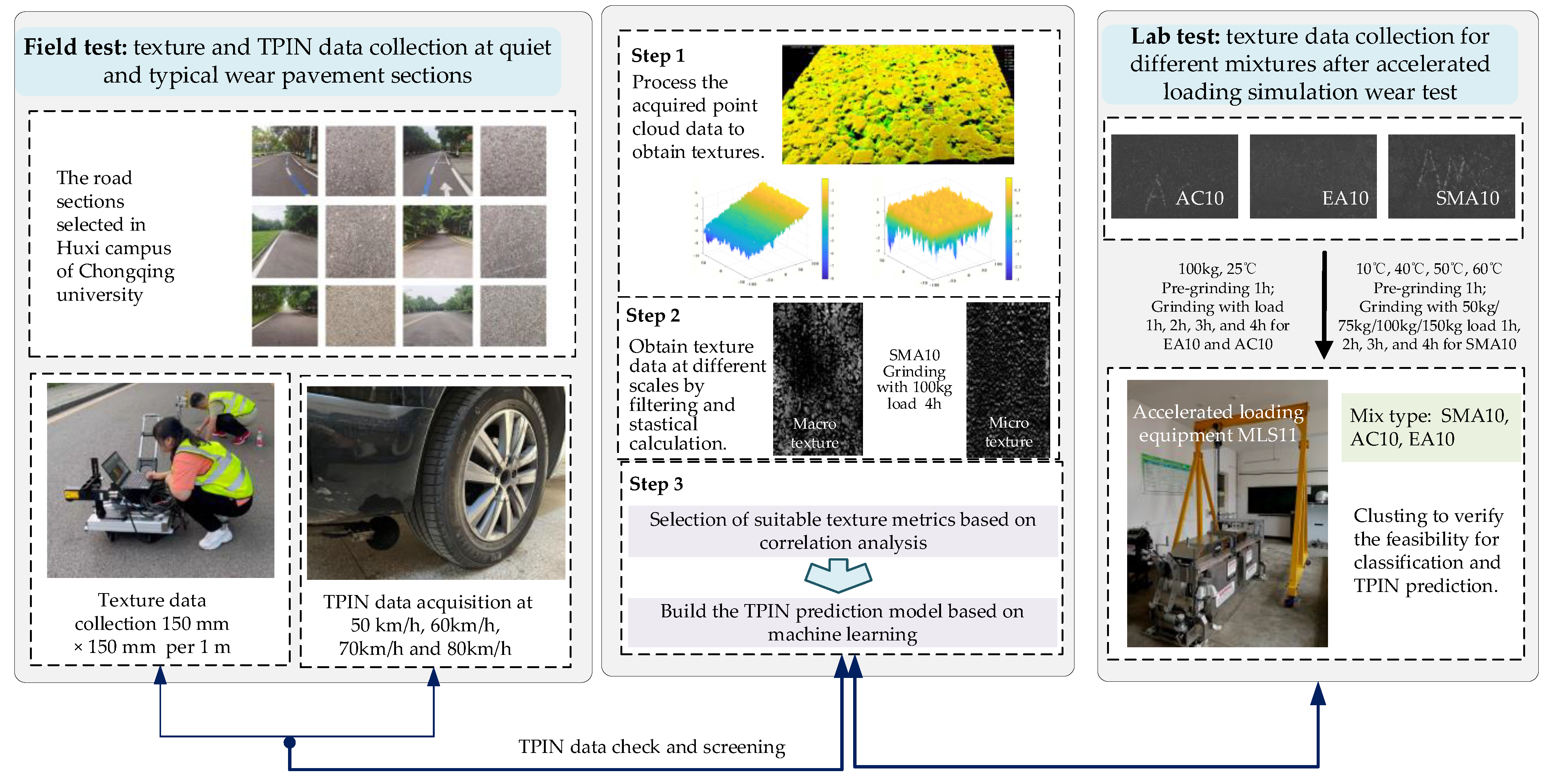
2.1. The Framework of This Study
2.2. Data Acquisition and Processing
2.2.1. Texture Data Collection
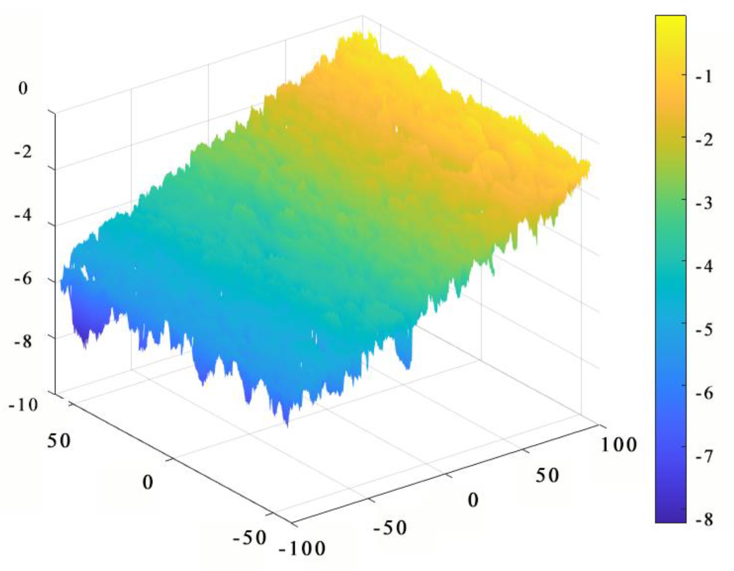
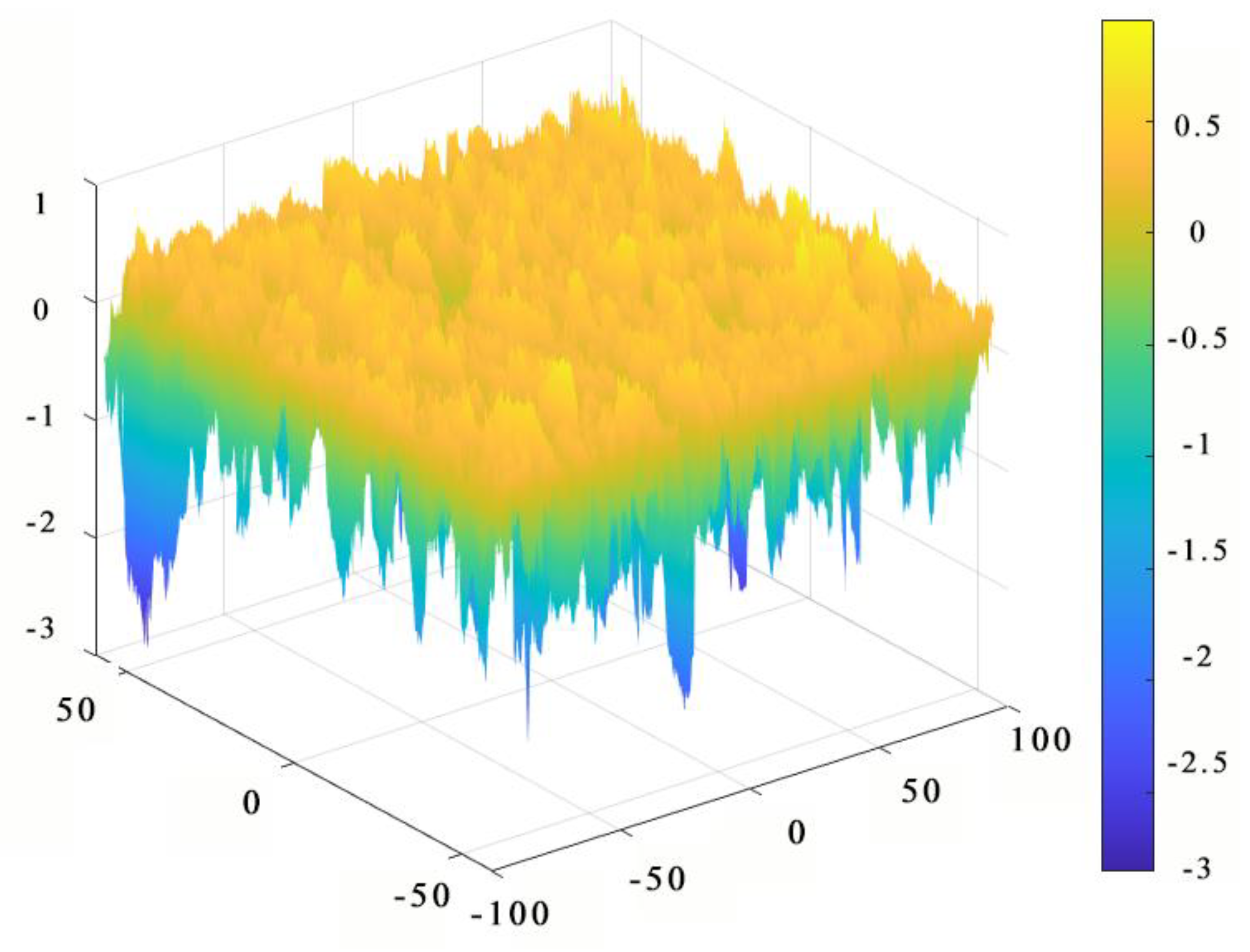
2.2.2. Texture Data Preprocess Method
2.2.3. Texture Metrics Calculation
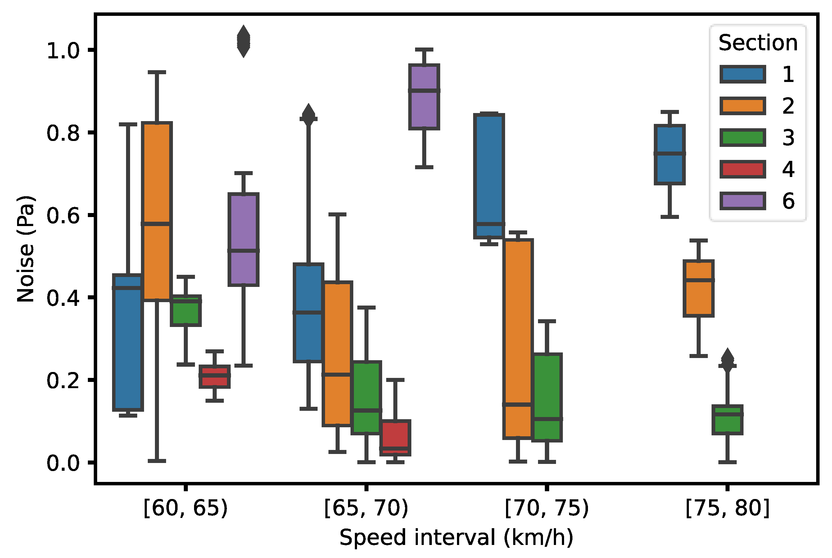
2.2.4. TPIN Data Collection and Data Representation Analysis
2.3. Texture Metrics Selection
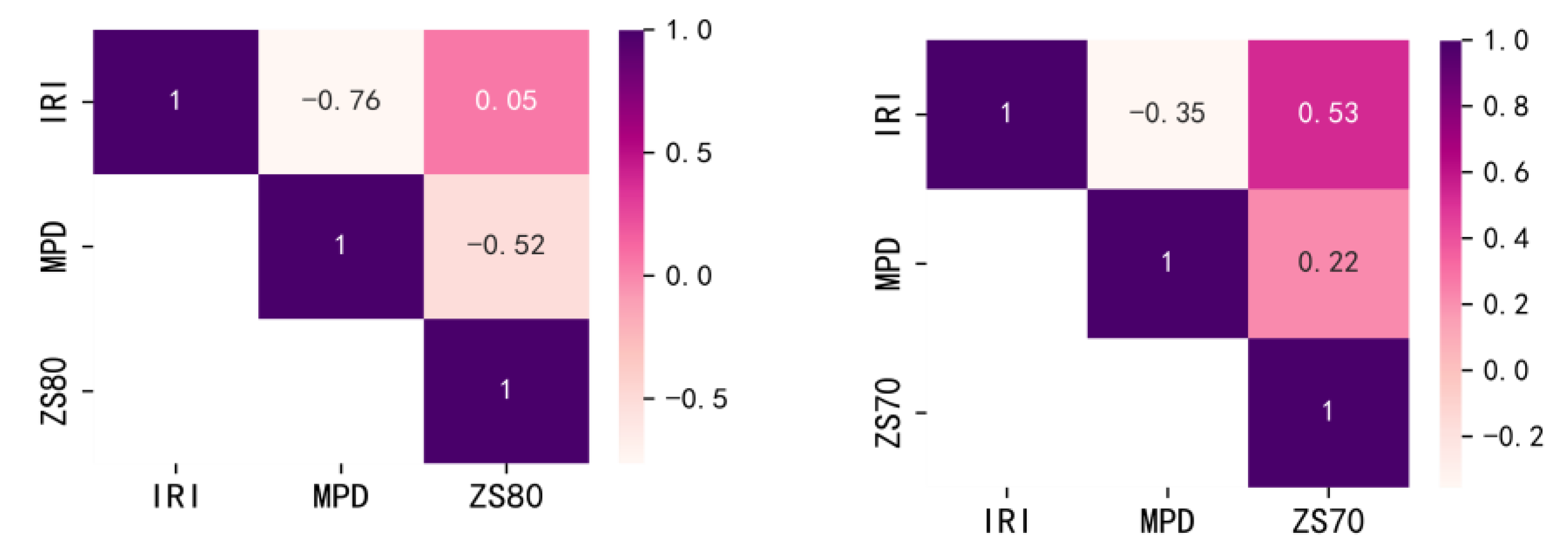
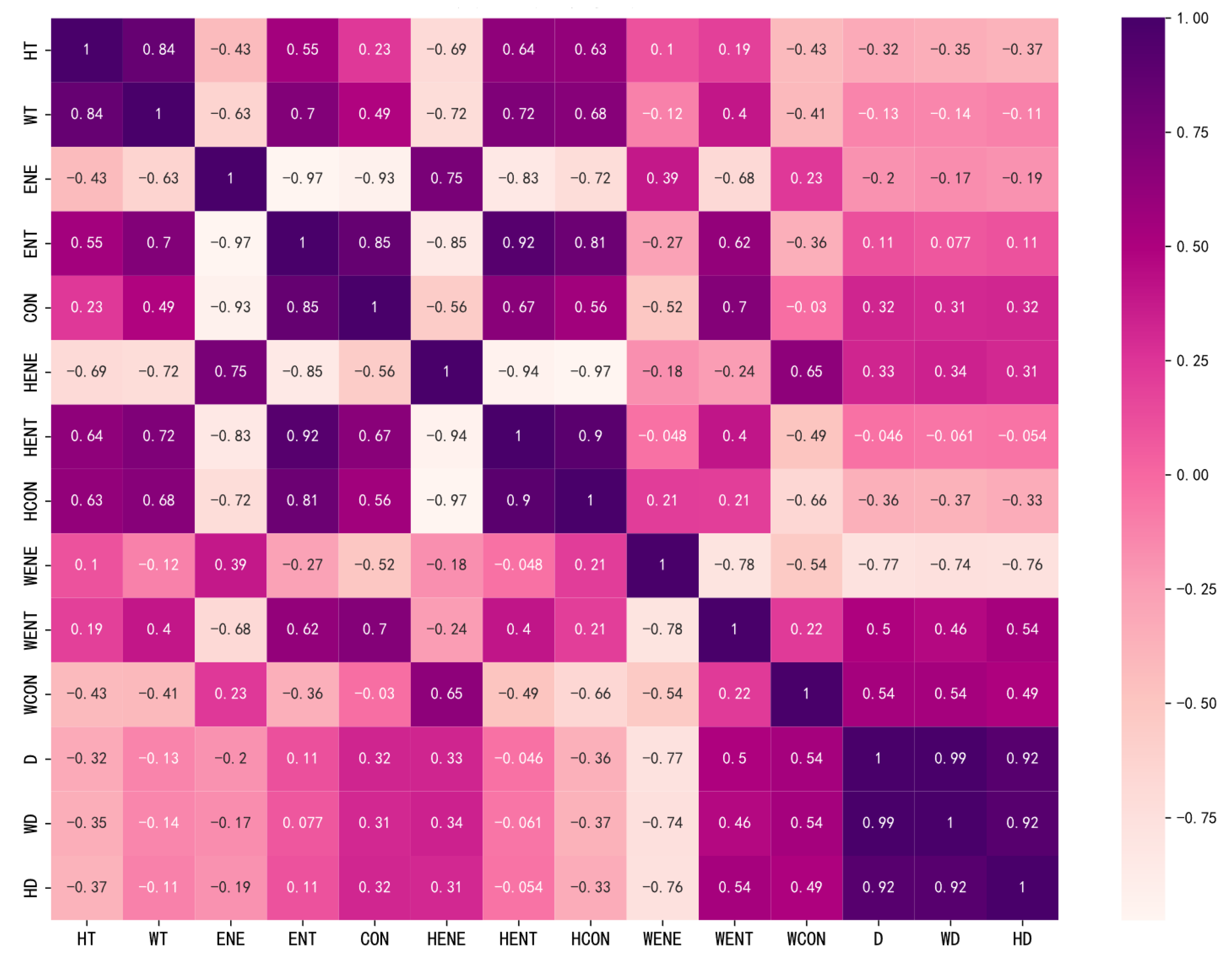
2.3.1. Texture Metrics Selection by Correlation Analysis
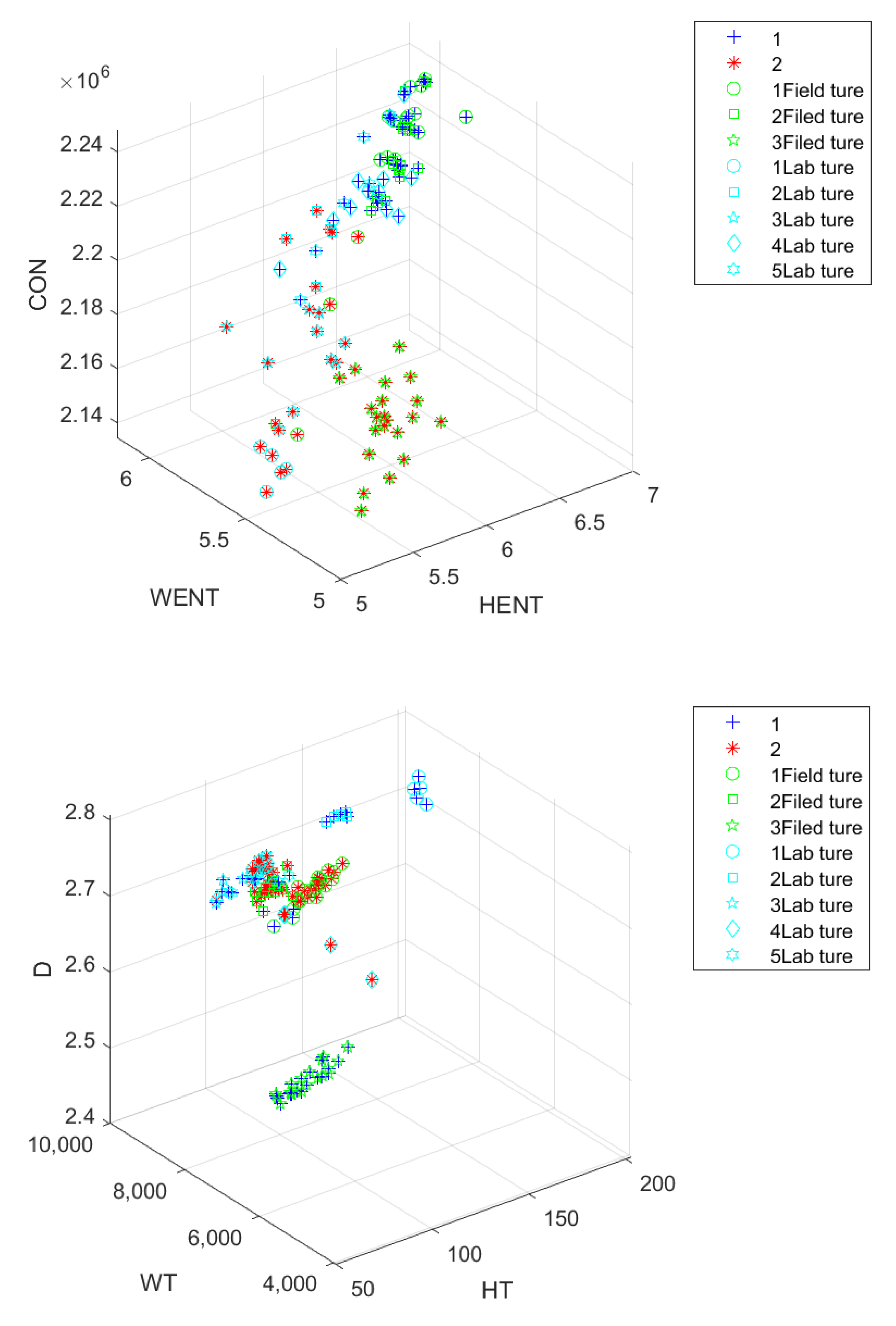
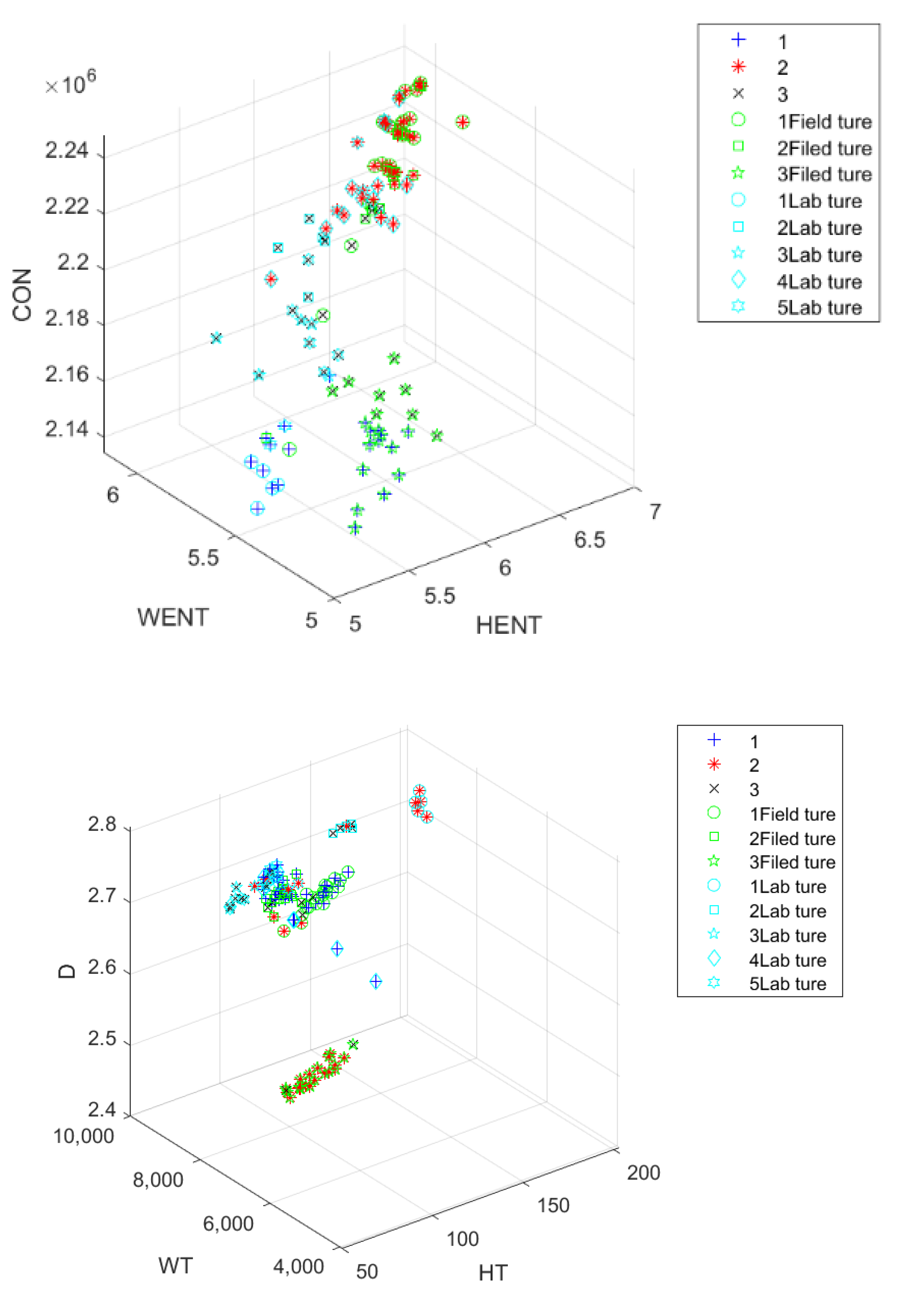
2.3.2. Application Validation of Texture Metrics Based on Clustering
2.4. Prediction Methods of TPIN
3. Results and Discussion
3.1. Section Selection Based on TPIN and Pavement Performance Detection Data
3.2. Spearman Correlation Analysis Results of Texture Metrics
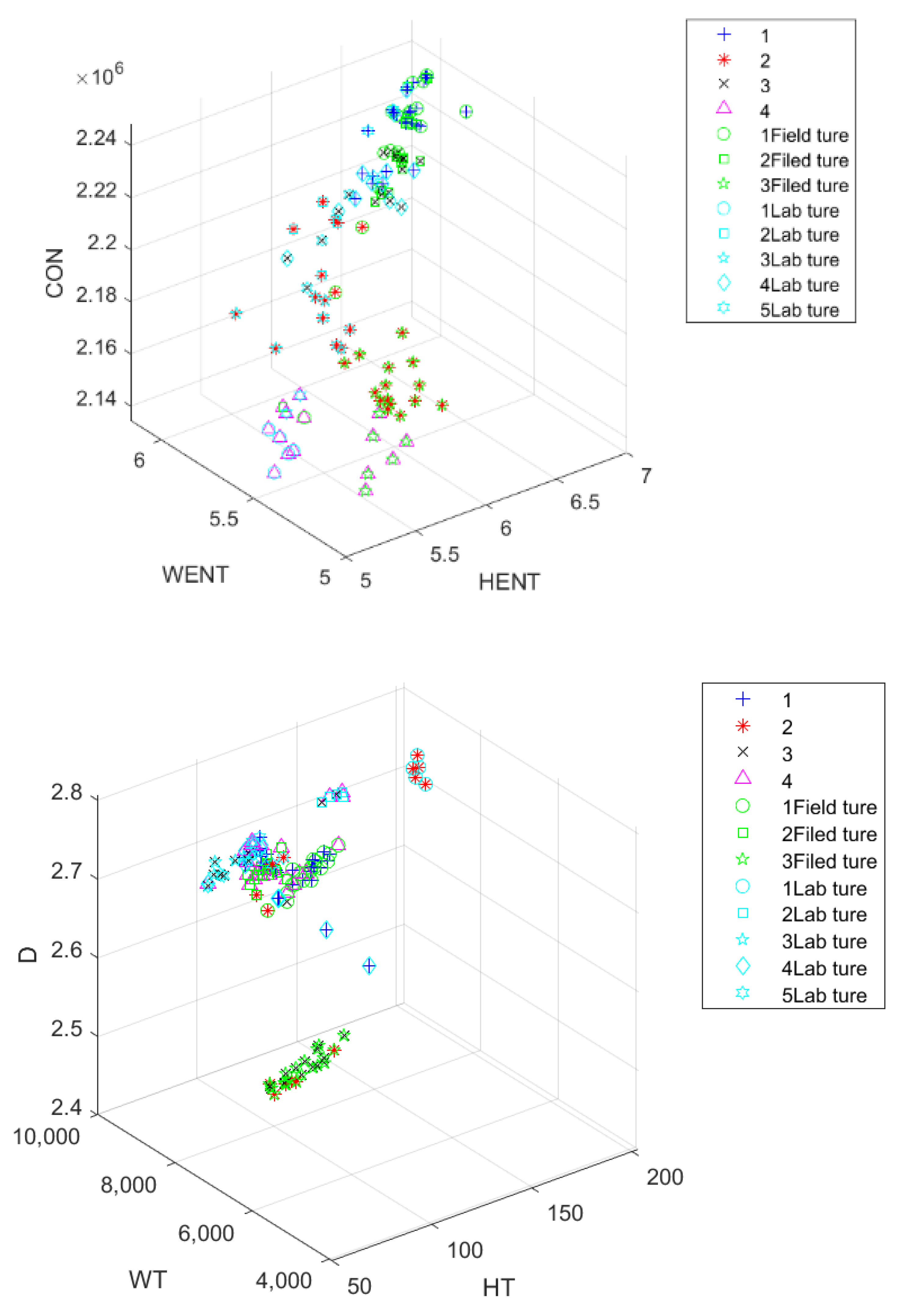
3.3. Clustering Results
3.3.1. The Internal Clustering Evaluation Results
3.3.2. The External Clustering Evaluation Results
3.3.3. The Clustering Results Analysis
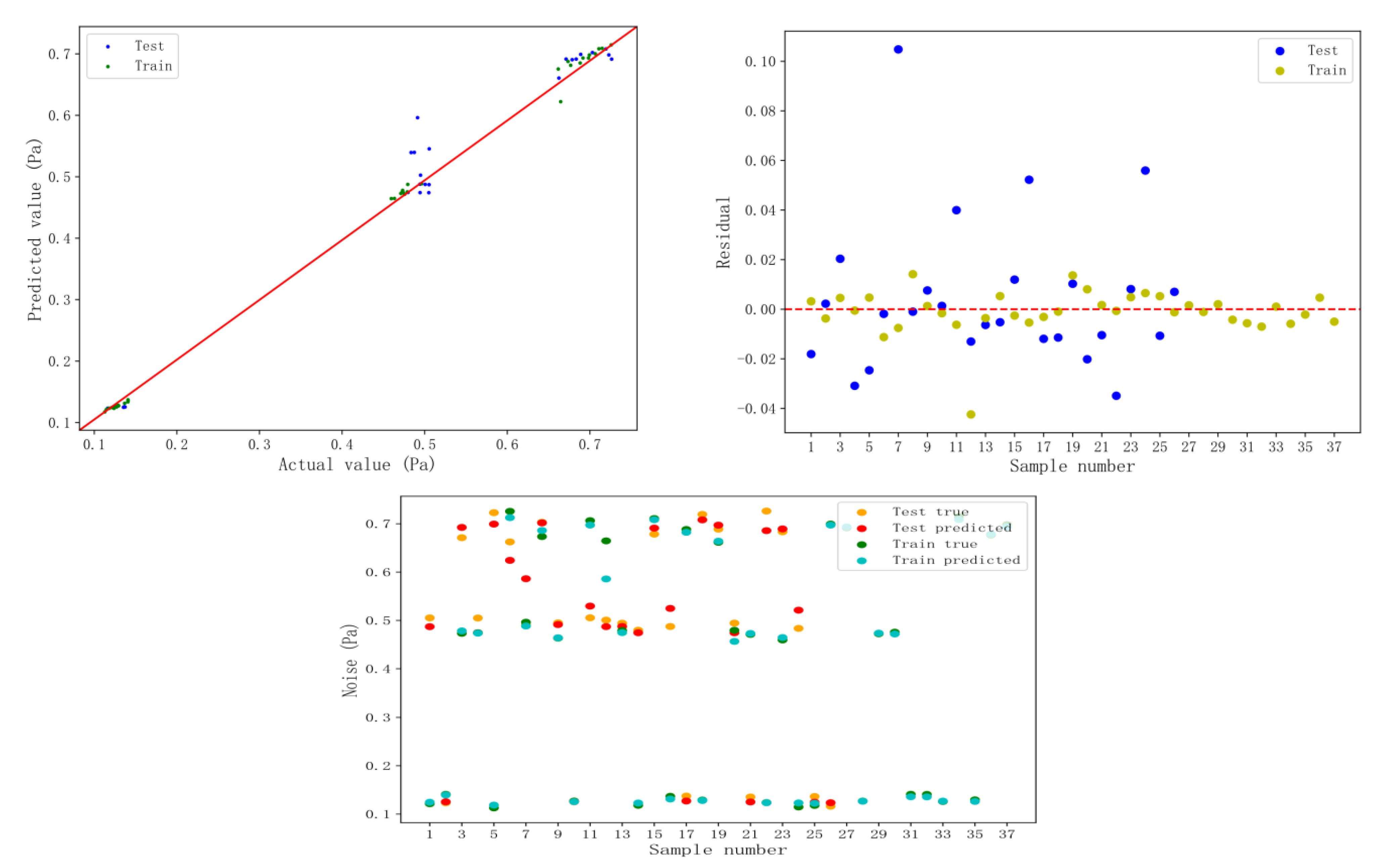
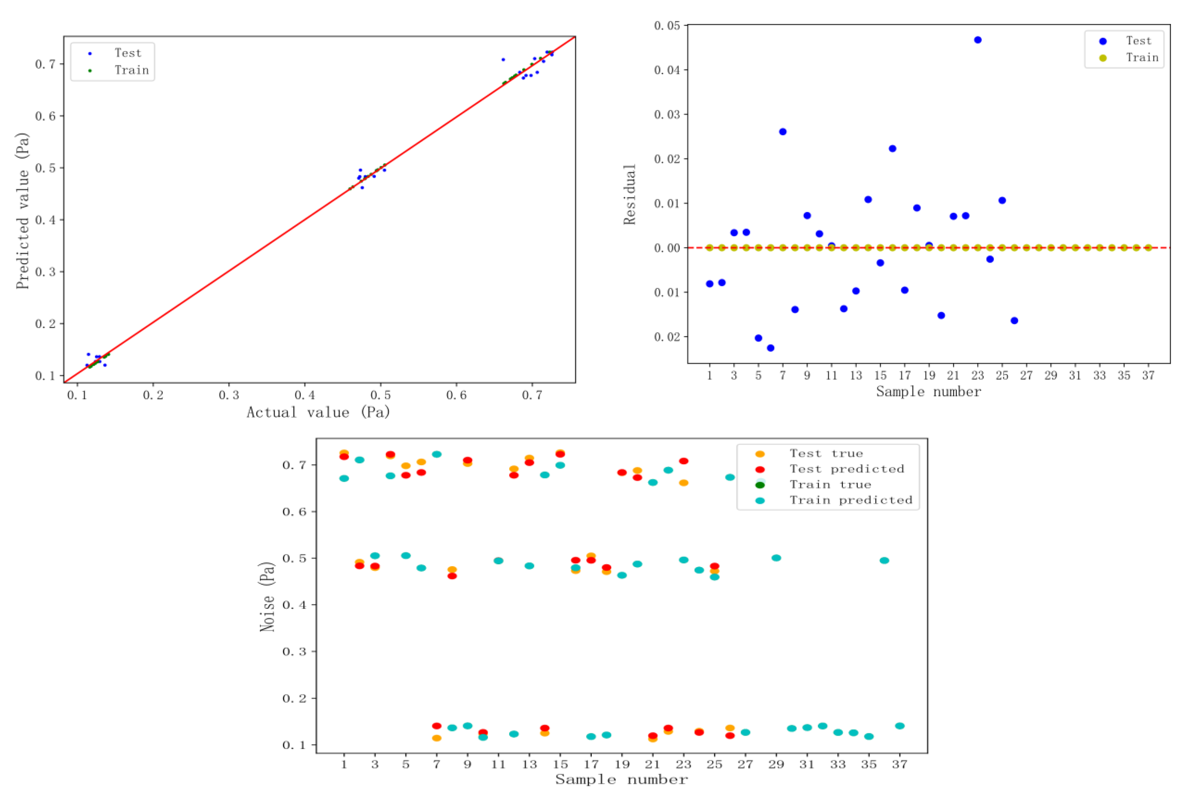
3.4. TPIN Prediction Results
4. Conclusions
- A method including preprocessing of 3D cloud data, pavement texture clustering, and TPIN prediction based on machine learning is proposed to predict TPIN.
- Macro- and microtexture statistics metrics are feasible for wear lab and field universal study, and the metrics combined can be used to sort different wear and TPIN levels.
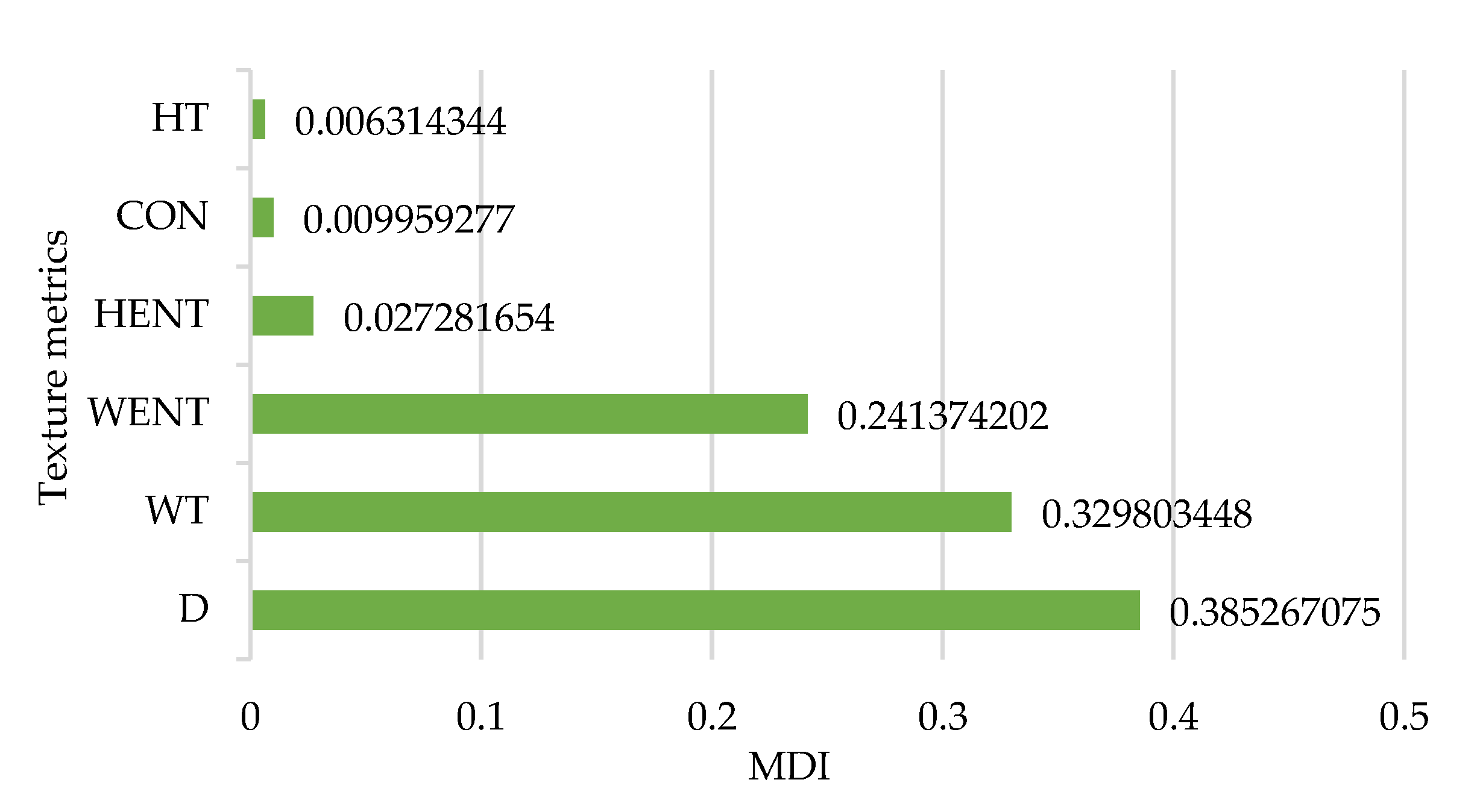
- The GBDT prediction model with D, WT, and WENT reaches a high accuracy (R2 = 0.9958, MSE = 0.0002).
Author Contributions
Funding
Institutional Review Board Statement
Informed Consent Statement
Data Availability Statement
Acknowledgments
Conflicts of Interest
Appendix A

| Section | Class | HT | WT | CON | HENT | WENT | D | K = 2 | K = 3 | K = 4 | N80 |
|---|---|---|---|---|---|---|---|---|---|---|---|
| 1 | 1 | 140.2518 | 9737.459 | 2,190,876 | 6.365243 | 5.948285 | 2.606582 | 2 | 3 | 1 | 0.6617 |
| 1 | 1 | 140.5601 | 9769.212 | 2,170,543 | 6.16111 | 5.935611 | 2.59399 | 2 | 1 | 2 | 0.6625 |
| 1 | 1 | 157.0259 | 9914.391 | 2,227,109 | 6.670939 | 5.864591 | 2.61801 | 1 | 2 | 3 | 0.6712 |
| 1 | 1 | 130.5765 | 9755.94 | 2,140,465 | 5.688288 | 5.747524 | 2.592336 | 2 | 1 | 4 | 0.6646 |
| 1 | 1 | 154.7143 | 9895.534 | 2,228,456 | 6.62285 | 5.983071 | 2.615811 | 1 | 2 | 3 | 0.6735 |
| 1 | 1 | 170.6463 | 9997.196 | 2,215,659 | 6.59751 | 5.930476 | 2.630418 | 1 | 3 | 1 | 0.6767 |
| 1 | 1 | 160.6162 | 9928.916 | 2,225,385 | 6.678157 | 5.926658 | 2.613039 | 1 | 2 | 3 | 0.6786 |
| 1 | 1 | 164.9753 | 9929.28 | 2,228,794 | 6.709074 | 5.944194 | 2.626497 | 1 | 2 | 3 | 0.6834 |
| 1 | 1 | 162.6561 | 9961.723 | 2,236,390 | 6.809056 | 5.723936 | 2.629737 | 1 | 2 | 3 | 0.6882 |
| 1 | 1 | 157.0566 | 9882.437 | 2,227,350 | 6.778483 | 5.965392 | 2.626263 | 1 | 2 | 3 | 0.6889 |
| 1 | 1 | 164.066 | 9922.555 | 2,240,394 | 6.815592 | 5.940327 | 2.618399 | 1 | 2 | 3 | 0.6982 |
| 1 | 1 | 154.3935 | 9856.267 | 2,237,931 | 6.745962 | 5.964423 | 2.605496 | 1 | 2 | 3 | 0.6994 |
| 1 | 1 | 164.066 | 9922.555 | 2,240,394 | 6.815592 | 5.940327 | 2.618399 | 1 | 2 | 3 | 0.6916 |
| 1 | 1 | 156.2884 | 9897.427 | 2,227,388 | 6.637929 | 5.971619 | 2.628652 | 1 | 2 | 3 | 0.7065 |
| 1 | 1 | 144.0166 | 9809.265 | 2,227,559 | 6.706778 | 5.95351 | 2.610949 | 1 | 2 | 3 | 0.7031 |
| 1 | 1 | 149.3278 | 9803.716 | 2,226,865 | 6.648029 | 5.974447 | 2.611791 | 1 | 2 | 3 | 0.7108 |
| 1 | 1 | 144.1535 | 9764.203 | 2,215,347 | 6.537224 | 5.960762 | 2.612284 | 1 | 3 | 1 | 0.7148 |
| 1 | 1 | 153.7648 | 9821.965 | 2,227,550 | 6.704577 | 5.952067 | 2.623179 | 1 | 2 | 3 | 0.7229 |
| 1 | 1 | 147.1195 | 9787.418 | 2,202,573 | 6.502314 | 5.959001 | 2.622824 | 1 | 3 | 1 | 0.7258 |
| 1 | 1 | 151.1389 | 9825.045 | 2,215,502 | 6.580022 | 5.957422 | 2.618354 | 1 | 3 | 1 | 0.7194 |
| 1 | 1 | 142.8201 | 9738.662 | 2,237,826 | 6.803949 | 5.951798 | 2.633391 | 1 | 2 | 3 | 0.7263 |
| 2 | 2 | 120.306 | 9496.202 | 2,141,056 | 5.652265 | 5.836816 | 2.629105 | 2 | 1 | 4 | 0.4795 |
| 2 | 2 | 123.4363 | 9423.833 | 2,225,290 | 6.705251 | 5.909514 | 2.66954 | 1 | 2 | 3 | 0.479 |
| 2 | 2 | 116.6561 | 9383.842 | 2,213,950 | 6.529906 | 5.855884 | 2.656537 | 1 | 3 | 1 | 0.4733 |
| 2 | 2 | 125.6373 | 9429.803 | 2,227,682 | 6.631201 | 5.915074 | 2.659555 | 1 | 2 | 3 | 0.4711 |
| 2 | 2 | 124.2467 | 9436.715 | 2,239,266 | 6.823183 | 5.940351 | 2.678627 | 1 | 2 | 3 | 0.4634 |
| 2 | 2 | 124.8888 | 9484.089 | 2,239,803 | 6.802336 | 5.938466 | 2.664685 | 1 | 2 | 3 | 0.4757 |
| 2 | 2 | 114.8213 | 9401.472 | 2,202,477 | 6.388935 | 5.893785 | 2.650193 | 1 | 3 | 1 | 0.4724 |
| 2 | 2 | 120.5244 | 9417.797 | 2,238,557 | 6.680337 | 5.941778 | 2.66832 | 1 | 2 | 3 | 0.4596 |
| 2 | 2 | 126.7114 | 9549.294 | 2,225,932 | 6.650289 | 5.929108 | 2.657626 | 1 | 2 | 3 | 0.4744 |
| 2 | 2 | 126.2311 | 9498.468 | 2,215,604 | 6.571671 | 5.899318 | 2.650512 | 1 | 3 | 1 | 0.4797 |
| 2 | 2 | 136.9934 | 9592.793 | 2,202,028 | 6.499463 | 5.952634 | 2.631535 | 1 | 3 | 1 | 0.4914 |
| 2 | 2 | 130.6252 | 9542.905 | 2,225,081 | 6.694389 | 5.927791 | 2.649595 | 1 | 2 | 3 | 0.4874 |
| 2 | 2 | 131.6491 | 9576.468 | 2,226,275 | 6.685228 | 5.944888 | 2.645004 | 1 | 2 | 3 | 0.4835 |
| 2 | 2 | 128.2213 | 9510.897 | 2,215,332 | 6.586884 | 5.930047 | 2.652833 | 1 | 3 | 1 | 0.495 |
| 2 | 2 | 120.996 | 9395.484 | 2,213,502 | 6.621387 | 5.916992 | 2.655977 | 1 | 3 | 1 | 0.4944 |
| 2 | 2 | 118.0208 | 9374.048 | 2,215,721 | 6.576274 | 5.885727 | 2.660711 | 1 | 3 | 1 | 0.4963 |
| 2 | 2 | 116.7086 | 9373.504 | 2,202,736 | 6.46337 | 5.916607 | 2.656968 | 1 | 3 | 1 | 0.4943 |
| 2 | 2 | 118.1459 | 9336.264 | 2,213,803 | 6.566077 | 5.890992 | 2.667591 | 1 | 3 | 1 | 0.5006 |
| 2 | 2 | 121.5127 | 9397.591 | 2,203,390 | 6.499117 | 5.904437 | 2.663514 | 1 | 3 | 1 | 0.505 |
| 2 | 2 | 111.4096 | 9294.882 | 2,215,074 | 6.571895 | 5.920085 | 2.669541 | 1 | 3 | 1 | 0.5053 |
| 2 | 2 | 133.3873 | 9535.165 | 2,213,571 | 6.673446 | 5.870046 | 2.675986 | 1 | 3 | 1 | 0.5055 |
| 3 | 3 | 118.8022 | 8190.827 | 2,170,419 | 5.838518 | 5.118374 | 2.459816 | 2 | 1 | 2 | 0.1363 |
| 3 | 3 | 138.5395 | 8193.125 | 2,181,998 | 5.958741 | 5.42493 | 2.47402 | 2 | 1 | 2 | 0.1408 |
| 3 | 3 | 126.7313 | 8230.696 | 2,162,734 | 5.890374 | 5.301612 | 2.471123 | 2 | 1 | 2 | 0.1409 |
| 3 | 3 | 103.3065 | 7897.602 | 2,162,401 | 5.715989 | 5.316755 | 2.453879 | 2 | 1 | 2 | 0.1373 |
| 3 | 3 | 110.7464 | 8109.603 | 2,145,140 | 5.700261 | 5.280097 | 2.444492 | 2 | 1 | 4 | 0.1407 |
| 3 | 3 | 109.8774 | 7937.153 | 2,153,412 | 5.622871 | 5.326607 | 2.449603 | 2 | 1 | 4 | 0.1367 |
| 3 | 3 | 124.7071 | 8001.231 | 2,170,730 | 5.863384 | 5.426774 | 2.463782 | 2 | 1 | 2 | 0.1294 |
| 3 | 3 | 120.4148 | 7935.903 | 2,162,511 | 5.773219 | 5.429787 | 2.46034 | 2 | 1 | 2 | 0.1353 |
| 3 | 3 | 93.96805 | 7802.107 | 2,180,690 | 5.824387 | 5.265382 | 2.463394 | 2 | 1 | 2 | 0.127 |
| 3 | 3 | 94.80948 | 7806.527 | 2,166,863 | 5.658132 | 5.314213 | 2.459358 | 2 | 1 | 2 | 0.129 |
| 3 | 3 | 99.93752 | 7732.5 | 2,171,267 | 5.716613 | 5.328969 | 2.463718 | 2 | 1 | 2 | 0.1253 |
| 3 | 3 | 102.6348 | 7834.169 | 2,138,417 | 5.480241 | 5.259559 | 2.456323 | 2 | 1 | 4 | 0.1234 |
| 3 | 3 | 99.65145 | 7693.064 | 2,161,535 | 5.742149 | 5.268382 | 2.477157 | 2 | 1 | 2 | 0.1238 |
| 3 | 3 | 114.0515 | 8022.764 | 2,162,486 | 5.759748 | 5.337354 | 2.451916 | 2 | 1 | 2 | 0.1269 |
| 3 | 3 | 133.6847 | 8192.826 | 2,153,492 | 5.814196 | 5.43795 | 2.460119 | 2 | 1 | 4 | 0.126 |
| 3 | 3 | 99.31789 | 7972.859 | 2,153,083 | 5.743936 | 5.239729 | 2.442288 | 2 | 1 | 4 | 0.1213 |
| 3 | 3 | 96.88123 | 7957.785 | 2,144,846 | 5.490411 | 5.253704 | 2.458167 | 2 | 1 | 4 | 0.1179 |
| 3 | 3 | 123.9664 | 8130.17 | 2,170,655 | 5.874836 | 5.267573 | 2.472092 | 2 | 1 | 2 | 0.1181 |
| 3 | 3 | 127.7747 | 8133.874 | 2,162,651 | 5.777118 | 5.365302 | 2.450702 | 2 | 1 | 2 | 0.1147 |
| 3 | 3 | 118.9286 | 7976.812 | 2,171,025 | 5.689691 | 5.532551 | 2.457837 | 2 | 1 | 2 | 0.1163 |
| 3 | 3 | 109.5175 | 7934.195 | 2,172,858 | 5.78724 | 5.521902 | 2.467659 | 2 | 1 | 2 | 0.1127 |
| Temperature (℃) | Load (kg) | Grid Time (h) | Mix Type | Class | HT | WT | CON | HENT | WENT | D | K = 2 | K = 3 | K = 4 | K = 5 |
|---|---|---|---|---|---|---|---|---|---|---|---|---|---|---|
| 25 | 100 | 1 | EA10 | 4 | 200.1252 | 9474.22 | 2,142,466 | 5.398496 | 5.661241 | 2.733111 | 2 | 2 | 3 | 2 |
| 25 | 100 | 2 | EA10 | 4 | 197.8918 | 9478.957 | 2,143,549 | 5.387827 | 5.710816 | 2.718602 | 2 | 2 | 3 | 2 |
| 25 | 100 | 3 | EA10 | 4 | 202.5992 | 9550.427 | 2,137,786 | 5.453854 | 5.628504 | 2.713419 | 2 | 2 | 3 | 2 |
| 25 | 100 | 4 | EA10 | 4 | 200.4735 | 9532.335 | 2,143,087 | 5.312544 | 5.547858 | 2.702988 | 2 | 2 | 3 | 2 |
| 25 | 100 | 1 | EA10 | 4 | 203.5031 | 9428.059 | 2,134,256 | 5.277661 | 5.598742 | 2.694699 | 2 | 2 | 3 | 2 |
| 25 | 100 | 3 | AC10 | 5 | 134.4078 | 8160.089 | 2,171,093 | 6.211048 | 6.047009 | 2.785007 | 2 | 1 | 4 | 1 |
| 25 | 100 | 1 | AC10 | 5 | 117.052 | 7656.542 | 2,186,354 | 6.126969 | 6.135854 | 2.806571 | 1 | 1 | 2 | 1 |
| 25 | 100 | 1 | AC10 | 5 | 125.8476 | 7895.707 | 2,190,935 | 6.371675 | 6.162665 | 2.798043 | 1 | 1 | 2 | 1 |
| 25 | 100 | 2 | AC10 | 5 | 139.006 | 8244.898 | 2,192,201 | 6.276161 | 6.023843 | 2.775359 | 1 | 1 | 2 | 1 |
| 25 | 100 | 4 | AC10 | 5 | 137.244 | 8165.502 | 2,191,308 | 6.277131 | 6.015132 | 2.784678 | 1 | 1 | 2 | 1 |
| 25 | 50 | 1 | SMA10 | 6 | 61.96747 | 7761.138 | 2,183,390 | 5.259744 | 5.576053 | 2.748872 | 1 | 1 | 2 | 1 |
| 25 | 75 | 1 | SMA10 | 6 | 80.415 | 8002.265 | 2,165,689 | 5.873896 | 5.68852 | 2.756023 | 2 | 2 | 4 | 1 |
| 25 | 50 | 2 | SMA10 | 6 | 65.62519 | 7783.155 | 2,186,631 | 5.268074 | 5.795175 | 2.758699 | 1 | 1 | 2 | 1 |
| 25 | 50 | 3 | SMA10 | 6 | 66.72891 | 7817.642 | 2,188,823 | 5.698766 | 5.696648 | 2.772231 | 1 | 1 | 2 | 1 |
| 25 | 75 | 2 | SMA10 | 6 | 89.77065 | 8134.768 | 2,188,164 | 5.731191 | 5.666633 | 2.742637 | 1 | 1 | 2 | 1 |
| 25 | 100 | 1 | SMA10 | 7 | 68.5346 | 3916.921 | 2,226,383 | 5.874341 | 5.615758 | 2.758084 | 1 | 3 | 1 | 5 |
| 25 | 150 | 1 | SMA10 | 7 | 99.11652 | 8313.325 | 2,238,468 | 6.441615 | 5.832935 | 2.743714 | 1 | 3 | 1 | 5 |
| 25 | 50 | 4 | SMA10 | 7 | 64.39665 | 7883.11 | 2,205,752 | 5.53187 | 5.723417 | 2.746018 | 1 | 1 | 2 | 4 |
| 25 | 100 | 2 | SMA10 | 7 | 73.08235 | 5278.396 | 2,231,365 | 5.970311 | 5.596111 | 2.75817 | 1 | 3 | 1 | 5 |
| 25 | 75 | 3 | SMA10 | 7 | 90.20172 | 8237.601 | 2,215,546 | 6.220091 | 5.689277 | 2.752201 | 1 | 3 | 1 | 4 |
| 25 | 75 | 4 | SMA10 | 7 | 90.27892 | 8238.604 | 2,230,901 | 6.258402 | 5.585971 | 2.734297 | 1 | 3 | 1 | 5 |
| 25 | 100 | 3 | SMA10 | 7 | 74.12594 | 6561.373 | 2,229,072 | 6.0399 | 5.699512 | 2.757991 | 1 | 3 | 1 | 5 |
| 25 | 150 | 2 | SMA10 | 7 | 92.34798 | 8239.015 | 2,248,238 | 6.473895 | 5.791404 | 2.748601 | 1 | 3 | 1 | 3 |
| 25 | 100 | 4 | SMA10 | 7 | 74.5372 | 6560.45 | 2,229,131 | 6.054549 | 5.602095 | 2.75715 | 1 | 3 | 1 | 5 |
| 10 | 100 | 1 | SMA10 | 7 | 85.94515 | 7801.888 | 2,207,245 | 6.066941 | 5.84916 | 2.776292 | 1 | 1 | 2 | 4 |
| 40 | 100 | 1 | SMA10 | 7 | 102.0044 | 8446.173 | 2,215,685 | 6.226914 | 5.630642 | 2.74203 | 1 | 3 | 1 | 4 |
| 40 | 100 | 2 | SMA10 | 7 | 103.6456 | 8540.191 | 2,232,364 | 6.10359 | 5.619615 | 2.722978 | 1 | 3 | 1 | 5 |
| 25 | 150 | 3 | SMA10 | 8 | 97.4696 | 8329.697 | 2,239,223 | 6.441555 | 5.839455 | 2.74283 | 1 | 3 | 1 | 5 |
| 25 | 150 | 4 | SMA10 | 8 | 90.91534 | 8315.082 | 2,232,870 | 6.297493 | 5.864532 | 2.74015 | 1 | 3 | 1 | 5 |
| 10 | 100 | 2 | SMA10 | 8 | 84.76578 | 7781.25 | 2,198,559 | 5.950772 | 5.850172 | 2.777894 | 1 | 1 | 2 | 4 |
| 60 | 100 | 1 | SMA10 | 8 | 91.1343 | 8198.318 | 2,174,016 | 5.724007 | 5.598527 | 2.749057 | 2 | 1 | 4 | 1 |
| 10 | 100 | 3 | SMA10 | 8 | 84.99197 | 7802.974 | 2,212,197 | 6.142412 | 5.848673 | 2.781691 | 1 | 3 | 1 | 4 |
| 40 | 100 | 3 | SMA10 | 8 | 114.7557 | 8531.808 | 2,144,505 | 5.563857 | 5.749093 | 2.710942 | 2 | 2 | 3 | 2 |
| 10 | 100 | 4 | SMA10 | 8 | 89.43663 | 7839.255 | 2,223,554 | 6.173675 | 5.741891 | 2.78192 | 1 | 3 | 1 | 5 |
| 40 | 100 | 4 | SMA10 | 8 | 112.0517 | 8666.278 | 2,149,006 | 5.667467 | 5.753685 | 2.701373 | 2 | 2 | 3 | 2 |
| 60 | 100 | 2 | SMA10 | 8 | 90.15488 | 8182.348 | 2,194,519 | 5.619295 | 5.679922 | 2.738758 | 1 | 1 | 2 | 1 |
| 60 | 100 | 3 | SMA10 | 8 | 77.39062 | 8219.836 | 2,179,930 | 5.749463 | 5.691116 | 2.734488 | 2 | 1 | 4 | 1 |
| 60 | 100 | 4 | SMA10 | 8 | 79.05924 | 8229.404 | 2,183,417 | 5.724156 | 5.529839 | 2.73144 | 1 | 1 | 2 | 1 |
| Sample Number | Items | Class | K = 2 | K = 3 | K = 4 |
|---|---|---|---|---|---|
| 1 | 1 | 1 | 2 | 3 | 3 |
| 2 | 1 | 1 | 1 | 1 | 4 |
| 3 | 1 | 1 | 1 | 2 | 4 |
| 4 | 1 | 1 | 1 | 2 | 4 |
| 5 | 1 | 1 | 1 | 2 | 4 |
| 6 | 1 | 1 | 1 | 2 | 2 |
| 7 | 1 | 1 | 1 | 2 | 2 |
| 8 | 1 | 1 | 1 | 2 | 2 |
| 9 | 1 | 1 | 1 | 2 | 2 |
| 10 | 1 | 1 | 1 | 2 | 2 |
| 11 | 1 | 1 | 1 | 2 | 2 |
| 12 | 1 | 1 | 1 | 2 | 2 |
| 13 | 1 | 1 | 1 | 2 | 2 |
| 14 | 1 | 1 | 1 | 2 | 2 |
| 15 | 1 | 1 | 1 | 2 | 2 |
| 16 | 1 | 1 | 1 | 2 | 2 |
| 17 | 1 | 1 | 1 | 2 | 2 |
| 18 | 1 | 1 | 1 | 2 | 2 |
| 19 | 1 | 1 | 1 | 2 | 2 |
| 20 | 1 | 1 | 2 | 1 | 1 |
| 21 | 1 | 1 | 2 | 1 | 1 |
| 22 | 2 | 2 | 2 | 3 | 3 |
| 23 | 2 | 2 | 1 | 2 | 4 |
| 24 | 2 | 2 | 1 | 1 | 4 |
| 25 | 2 | 2 | 1 | 2 | 4 |
| 26 | 2 | 2 | 1 | 2 | 4 |
| 27 | 2 | 2 | 1 | 2 | 4 |
| 28 | 2 | 2 | 1 | 1 | 4 |
| 29 | 2 | 2 | 1 | 2 | 4 |
| 30 | 2 | 2 | 1 | 2 | 4 |
| 31 | 2 | 2 | 1 | 1 | 4 |
| 32 | 2 | 2 | 1 | 2 | 4 |
| 33 | 2 | 2 | 1 | 1 | 4 |
| 34 | 2 | 2 | 1 | 2 | 4 |
| 35 | 2 | 2 | 1 | 2 | 2 |
| 36 | 2 | 2 | 1 | 2 | 2 |
| 37 | 2 | 2 | 1 | 2 | 2 |
| 38 | 2 | 2 | 1 | 2 | 2 |
| 39 | 2 | 2 | 1 | 2 | 2 |
| 40 | 2 | 2 | 1 | 2 | 2 |
| 41 | 2 | 2 | 1 | 2 | 2 |
| 42 | 2 | 2 | 1 | 2 | 2 |
| 43 | 3 | 3 | 2 | 3 | 1 |
| 44 | 3 | 3 | 2 | 3 | 3 |
| 45 | 3 | 3 | 2 | 3 | 3 |
| 46 | 3 | 3 | 2 | 3 | 3 |
| 47 | 3 | 3 | 2 | 3 | 1 |
| 48 | 3 | 3 | 2 | 3 | 1 |
| 49 | 3 | 3 | 2 | 3 | 3 |
| 50 | 3 | 3 | 2 | 3 | 1 |
| 51 | 3 | 3 | 2 | 3 | 3 |
| 52 | 3 | 3 | 2 | 3 | 3 |
| 53 | 3 | 3 | 2 | 3 | 1 |
| 54 | 3 | 3 | 2 | 3 | 1 |
| 55 | 3 | 3 | 2 | 1 | 1 |
| 56 | 3 | 3 | 2 | 1 | 1 |
| 57 | 3 | 3 | 2 | 1 | 1 |
| 58 | 3 | 3 | 2 | 1 | 1 |
| 59 | 3 | 3 | 2 | 3 | 1 |
| 60 | 3 | 3 | 2 | 1 | 1 |
| 61 | 3 | 3 | 2 | 1 | 1 |
| 62 | 3 | 3 | 2 | 1 | 1 |
| 63 | 3 | 3 | 2 | 1 | 1 |
| 64 | EA10 | 4 | 2 | 3 | 3 |
| 65 | EA10 | 4 | 2 | 3 | 3 |
| 66 | EA10 | 4 | 2 | 3 | 3 |
| 67 | EA10 | 4 | 2 | 3 | 3 |
| 68 | EA10 | 4 | 2 | 3 | 3 |
| 69 | AC10 | 5 | 2 | 1 | 1 |
| 70 | AC10 | 5 | 2 | 1 | 1 |
| 71 | AC10 | 5 | 2 | 1 | 1 |
| 72 | AC10 | 5 | 2 | 1 | 1 |
| 73 | AC10 | 5 | 2 | 1 | 1 |
| 74 | SMA10 | 6 | 2 | 1 | 1 |
| 75 | SMA10 | 6 | 2 | 3 | 1 |
| 76 | SMA10 | 6 | 2 | 1 | 1 |
| 77 | SMA10 | 6 | 2 | 1 | 1 |
| 78 | SMA10 | 6 | 2 | 1 | 1 |
| 79 | SMA10 | 7 | 1 | 2 | 2 |
| 80 | SMA10 | 7 | 1 | 2 | 2 |
| 81 | SMA10 | 7 | 1 | 1 | 4 |
| 82 | SMA10 | 7 | 1 | 2 | 2 |
| 83 | SMA10 | 7 | 1 | 2 | 4 |
| 84 | SMA10 | 7 | 1 | 2 | 2 |
| 85 | SMA10 | 7 | 1 | 2 | 2 |
| 86 | SMA10 | 7 | 1 | 2 | 2 |
| 87 | SMA10 | 7 | 1 | 2 | 2 |
| 88 | SMA10 | 7 | 1 | 2 | 4 |
| 89 | SMA10 | 7 | 1 | 2 | 4 |
| 90 | SMA10 | 7 | 1 | 2 | 2 |
| 91 | SMA10 | 8 | 1 | 2 | 2 |
| 92 | SMA10 | 8 | 1 | 2 | 2 |
| 93 | SMA10 | 8 | 1 | 1 | 4 |
| 94 | SMA10 | 8 | 2 | 1 | 1 |
| 95 | SMA10 | 8 | 1 | 2 | 4 |
| 96 | SMA10 | 8 | 2 | 3 | 3 |
| 97 | SMA10 | 8 | 1 | 2 | 2 |
| 98 | SMA10 | 8 | 2 | 3 | 3 |
| 99 | SMA10 | 8 | 1 | 1 | 4 |
| 100 | SMA10 | 8 | 2 | 1 | 1 |
| 101 | SMA10 | 8 | 2 | 1 | 1 |
References
- Li, Q.; Qiao, F.; Lei, Y. Impacts of pavement types on in-vehicle noise and human health. J. Air Waste Manag. Assoc. 2016, 66, 87–96. [Google Scholar] [CrossRef] [PubMed]
- Abu Dabous, S.; Zeiada, W.; Zayed, T.; Al-Ruzouq, R. Sustainability-informed multi-criteria decision support framework for ranking and prioritization of pavement sections. J. Clean. Prod. 2019, 244, 118755. [Google Scholar] [CrossRef]
- Yang, W.; He, J.; He, C.; Cai, M. Evaluation of urban traffic noise pollution based on noise maps. Transp. Res. Part D Transp. Environ. 2020, 87, 102516. [Google Scholar] [CrossRef]
- Khajehvand, M.; Rassafi, A.A.; Mirbaha, B. Modeling traffic noise level near at-grade junctions: Roundabouts, T and cross intersections. Transp. Res. Part D Transp. Environ. 2021, 93, 102752. [Google Scholar] [CrossRef]
- Cao, R.; Leng, Z.; Yu, J.; Hsu, S.-C. Multi-objective optimization for maintaining low-noise pavement network system in Hong Kong. Transp. Res. Part D Transp. Environ. 2020, 88, 102573. [Google Scholar] [CrossRef]
- Nowoświat, A.; Sorociak, W.; Żuchowski, R. The impact of the application of thin emulsion mat microsurfacing on the level of noise in the environment. Constr. Build. Mater. 2020, 263, 120626. [Google Scholar] [CrossRef]
- Bernhard, R.; Wayson, R.L.; Haddock, J.; Neithalath, N.; El-Aassar, A.; Olek, J.; Pellinen, T.; Weiss, W.J. An Introduction to Tire/Pavement Noise of Asphalt Pavement; Institute of Safe, Quiet and Durable Highways, Purdue University: West Lafayette, IN, USA, 2005. [Google Scholar]
- Staiano, M.A. Tire–Pavement Noise and Pavement Texture. J. Transp. Eng. Part B Pavements 2018, 144, 04018034. [Google Scholar] [CrossRef]
- Ganji, M.R.; Golroo, A.; Sheikhzadeh, H.; Ghelmani, A.; Bidgoli, M.A. Dense-graded asphalt pavement macrotexture measurement using tire/road noise monitoring. Autom. Constr. 2019, 106, 102887. [Google Scholar] [CrossRef]
- Ganji, M.R.; Ghelmani, A.; Golroo, A.; Sheikhzadeh, H. Mean texture depth measurement with an acoustical-based apparatus using cepstral signal processing and support vector machine. Appl. Acoust. 2019, 161, 107168. [Google Scholar] [CrossRef]
- Mikhailenko, P.; Piao, Z.; Kakar, M.R.; Bueno, M.; Athari, S.; Pieren, R.; Heutschi, K.; Poulikakos, L. Low-Noise pavement technologies and evaluation techniques: A literature review. Int. J. Pavement Eng. 2020, 23, 1911–1934. [Google Scholar] [CrossRef]
- Chen, D.; Han, S.; Ren, X.; Ye, A.; Wang, W.; Su, Q.; Wang, T. Measuring the tyre/pavement noise using laboratory tyre rolling-down method. Int. J. Pavement Eng. 2019, 21, 1595–1605. [Google Scholar] [CrossRef]
- Han, S.; Peng, B.; Chu, L.; Fwa, T.F. In-door laboratory high-speed testing of tire-pavement noise. Int. J. Pavement Eng. 2020, 23, 321–331. [Google Scholar] [CrossRef]
- Li, T. A Review on Physical Mechanisms of Tire-Pavement Interaction Noise. SAE Int. J. Veh. Dyn. Stab. NVH 2019, 3, 87–112. [Google Scholar] [CrossRef]
- Chen, D.; Ling, C.; Wang, T.; Su, Q.; Ye, A. Prediction of tire-pavement noise of porous asphalt mixture based on mixture surface texture level and distributions. Constr. Build. Mater. 2018, 173, 801–810. [Google Scholar] [CrossRef]
- Zhang, H.; Liu, Z.; Meng, X. Noise reduction characteristics of asphalt pavement based on indoor simulation tests. Constr. Build. Mater. 2019, 215, 285–297. [Google Scholar] [CrossRef]
- Praticò, F.G.; Fedele, R.; Pellicano, G. Pavement FRFs and noise: A theoretical and experimental investigation. Constr. Build. Mater. 2021, 294, 123487. [Google Scholar] [CrossRef]
- Chen, J.; Yin, X.; Wang, H.; Ding, Y. Evaluation of durability and functional performance of porous polyurethane mixture in porous pavement. J. Clean. Prod. 2018, 188, 12–19. [Google Scholar] [CrossRef]
- Šernas, O.; Vaitkus, A.; Gražulytė, J.; Skrodenis, D.; Wasilewska, M.; Gierasimiuk, P. Development of low noise and durable semi-dense asphalt mixtures. Constr. Build. Mater. 2021, 293, 123413. [Google Scholar] [CrossRef]
- Vázquez, V.; Terán, F.; Huertas, P.; Paje, S. Field assessment of a Cold-In place-recycled pavement: Influence on rolling noise. J. Clean. Prod. 2018, 197, 154–162. [Google Scholar] [CrossRef]
- Dong, S.; Han, S.; Yin, Y.; Zhang, Z.; Yao, T. The method for accurate acquisition of pavement macro-texture and corresponding finite element model based on three-dimensional point cloud data. Constr. Build. Mater. 2021, 312, 125390. [Google Scholar] [CrossRef]
- Lou, K.; Xiao, P.; Kang, A.; Wu, Z.; Dong, X. Effects of asphalt pavement characteristics on traffic noise reduction in different frequencies. Transp. Res. Part D Transp. Environ. 2022, 106, 103259. [Google Scholar] [CrossRef]
- Li, Y.; Qin, Y.; Wang, H.; Xu, S.; Li, S. Study of Texture Indicators Applied to Pavement Wear Analysis Based on 3D Image Technology. Sensors 2022, 22, 4955. [Google Scholar] [CrossRef] [PubMed]
- Vázquez, V.F.; Terán, F.; Huertas, P.; Paje, S.E. Surface Aging Effect on Tire/Pavement Noise Medium-Term Evolution in a Medium-Size City. Coatings 2018, 8, 206. [Google Scholar] [CrossRef]
- Chen, L.; Cong, L.; Dong, Y.; Yang, G.; Tang, B.; Wang, X.; Gong, H. Investigation of influential factors of tire/pavement noise: A multilevel Bayesian analysis of full-scale track testing data. Constr. Build. Mater. 2021, 270, 121484. [Google Scholar] [CrossRef]
- Li, T. A state-of-the-art review of measurement techniques on tire–pavement interaction noise. Measurement 2018, 128, 325–351. [Google Scholar] [CrossRef]
- Li, T. Influencing Parameters on Tire–Pavement Interaction Noise: Review, Experiments, and Design Considerations. Designs 2018, 2, 38. [Google Scholar] [CrossRef]
- Bassil, M.B.L.; Cesbron, J.; Klein, P. Tyre/road noise: A piston approach for CFD modeling of air volume variation in a cylindrical road cavity. J. Sound Vib. 2019, 469, 115140. [Google Scholar] [CrossRef]
- Ding, Y.; Wang, H. FEM-BEM analysis of tyre-pavement noise on porous asphalt surfaces with different textures. Int. J. Pavement Eng. 2017, 20, 1090–1097. [Google Scholar] [CrossRef]
- Kleizienė, R.; Šernas, O.; Vaitkus, A.; Simanavičienė, R. Asphalt Pavement Acoustic Performance Model. Sustainability 2019, 11, 2938. [Google Scholar] [CrossRef]
- Yang, W.; Cai, M.; Luo, P. The calculation of road traffic noise spectrum based on the noise spectral characteristics of single vehicles. Appl. Acoust. 2019, 160, 107128. [Google Scholar] [CrossRef]
- Cao, R.; Leng, Z.; Hsu, S.-C.; Hung, W.-T. Modelling of the pavement acoustic longevity in Hong Kong through machine learning techniques. Transp. Res. Part D Transp. Environ. 2020, 83, 102366. [Google Scholar] [CrossRef]
- Matlack, G.R.; Horn, A.; Aldo, A.; Walubita, L.F.; Naik, B.; Khoury, I. Measuring surface texture of in-service asphalt pavement: Evaluation of two proposed hand-portable methods. Road Mater. Pavement Des. 2021, 2, 1–17. [Google Scholar] [CrossRef]
- Xin, Q.; Qian, Z.; Miao, Y.; Meng, L.; Wang, L. Three-dimensional characterisation of asphalt pavement macrotexture using laser scanner and micro element. Road Mater. Pavement Des. 2017, 18, 190–199. [Google Scholar] [CrossRef]
- Chen, J.; Huang, X.; Zheng, B.; Zhao, R.; Liu, X.; Cao, Q.; Zhu, S. Real-time identification system of asphalt pavement texture based on the close-range photogrammetry. Constr. Build. Mater. 2019, 226, 910–919. [Google Scholar] [CrossRef]
- Chen, D.; Sefidmazgi, N.R.; Bahia, H. Exploring the feasibility of evaluating asphalt pavement surface macro-texture using image-based texture analysis method. Road Mater. Pavement Des. 2014, 16, 405–420. [Google Scholar] [CrossRef]
- Chen, D. Evaluating asphalt pavement surface texture using 3D digital imaging. Int. J. Pavement Eng. 2018, 21, 416–427. [Google Scholar] [CrossRef]
- Dong, S.; Han, S.; Luo, Y.; Han, X.; Xu, O. Evaluation of tire-pavement noise based on three-dimensional pavement texture characteristics. Constr. Build. Mater. 2021, 306, 124935. [Google Scholar] [CrossRef]
- Weng, Z.; Xiang, H.; Lin, Y.; Liu, C.; Wu, D.; Du, Y. Pavement texture depth estimation using image-based multiscale features. Autom. Constr. 2022, 141, 104404. [Google Scholar] [CrossRef]
- Medeiros, M., Jr.; Babadopulos, L.; Maia, R.; Branco, V.C. 3D pavement macrotexture parameters from close range photogrammetry. Int. J. Pavement Eng. 2021, 1–15. [Google Scholar] [CrossRef]
- Standard No. 13473-4; Characterization of Pavement Texture by Use of Surface Profiles—Part 4: Spectral Analysis of Texture Profiles. ISO: Geneva, Switzerland.
- Arthur, D.; Vassilvitskii, S. K-means++: The Advantages of Careful Seeding. In Proceedings of the SODA ’07: Proceedings of the 18th Annual ACM-SIAM Symposium on Discrete Algorithms, New Orleans, LA, USA, 7–9 January 2007; pp. 1027–1035. [Google Scholar]
- Pal, N.; Biswas, J. Cluster validation using graph theoretic concepts. Pattern Recognit. 1997, 30, 847–857. [Google Scholar] [CrossRef]
- Nitya Sai, L.; Sai Shreya, M.; Anjan Subudhi, A.; Jaya Lakshmi, B.; Madhuri, K.B. Optimal K-Means Clustering Method Using Silhouette Coefficient. Int. J. Appl. Res. Inf. Technol. Comput. 2017, 8. [Google Scholar] [CrossRef]
- Robert, V.; Vasseur, Y.; Brault, V. Comparing High-Dimensional Partitions with the Co-clustering Adjusted Rand Index. J. Classif. 2020, 38, 158–186. [Google Scholar] [CrossRef]
- Hoang, T.; Do, T.-T.; Nguyen, T.V.; Cheung, N.-M. Multimodal Mutual Information Maximization: A Novel Approach for Unsupervised Deep Cross-Modal Hashing. IEEE Trans. Neural Netw. Learn. Syst. 2022; in press. [Google Scholar] [CrossRef] [PubMed]
- Luo, Z.; Wang, H.; Li, S. Prediction of International Roughness Index Based on Stacking Fusion Model. Sustainability 2022, 14, 6949. [Google Scholar] [CrossRef]
- Breiman, L. Manual on Setting Up, Using, and Understanding Random Forests v3.1. Technical Report. 2012. Available online: https://oz.berkeley.edu/users/breiman (accessed on 15 January 2022).


| Data | K | CH | DBI | SC |
|---|---|---|---|---|
| Field and Lab | 2 | 363.3304 | 0.4447 | 0.82252 |
| 3 | 372.1617 | 0.5443 | 0.6967 | |
| 4 | 483.8602 | 0.4473 | 0.7765 | |
| Field | 2 | 350.8164 | 0.3385 | 0.8969 |
| 3 | 335.7978 | 0.4866 | 0.8220 | |
| 4 | 476.5886 | 0.5122 | 0.8076 | |
| Lab | 2 | 68.6601 | 0.5620 | 0.6977 |
| 3 | 184.5086 | 0.3553 | 0.8225 | |
| 4 | 196.5702 | 0.5417 | 0.7037 | |
| 5 | 300.9437 | 0.4385 | 0.7904 |
| Data | K | RI | MI | Purity |
|---|---|---|---|---|
| Field and Lab | 2 | 0.6125 | 0.4870 | 0.4059 |
| 3 | 0.6715 | 0.4788 | 0.3762 | |
| 4 | 0.7366 | 0.6250 | 0.4653 | |
| Field | 2 | 0.7332 | 0.4712 | 0.6507 |
| 3 | 0.7639 | 0.5324 | 0.7460 | |
| 4 | 0.7363 | 0.5534 | 0.7460 | |
| Lab | 2 | 0.5348 | 0.2802 | 0.4474 |
| 3 | 0.6984 | 0.5520 | 0.5263 | |
| 4 | 0.7311 | 0.6209 | 0.5526 | |
| 5 | 0.7340 | 0.7492 | 0.5789 |
| The Prediction Model | MAPE | MSE | R2 | Data Description |
|---|---|---|---|---|
| RF | 0.0471 | 0.0009 | 0.9797 | Field test data of sound pressure |
| GBDT | 0.0376 | 0.0002 | 0.9958 | |
| SVM | 0.0824 | 0.0072 | 0.8688 | |
| F-test results of linear model [13] | / | / | 0.94 | Lab test, low speed (23.9 km/h) |
| Bayesian multilevel model [24] | / | / | 0.968 | Field test data of sound pressure |
Publisher’s Note: MDPI stays neutral with regard to jurisdictional claims in published maps and institutional affiliations. |
© 2022 by the authors. Licensee MDPI, Basel, Switzerland. This article is an open access article distributed under the terms and conditions of the Creative Commons Attribution (CC BY) license (https://creativecommons.org/licenses/by/4.0/).
Share and Cite
Wang, H.; Zhang, X.; Jiang, S. A Laboratory and Field Universal Estimation Method for Tire–Pavement Interaction Noise (TPIN) Based on 3D Image Technology. Sustainability 2022, 14, 12066. https://doi.org/10.3390/su141912066
Wang H, Zhang X, Jiang S. A Laboratory and Field Universal Estimation Method for Tire–Pavement Interaction Noise (TPIN) Based on 3D Image Technology. Sustainability. 2022; 14(19):12066. https://doi.org/10.3390/su141912066
Chicago/Turabian StyleWang, Hui, Xun Zhang, and Shengchuan Jiang. 2022. "A Laboratory and Field Universal Estimation Method for Tire–Pavement Interaction Noise (TPIN) Based on 3D Image Technology" Sustainability 14, no. 19: 12066. https://doi.org/10.3390/su141912066