Machine Learning Improvement of Streamflow Simulation by Utilizing Remote Sensing Data and Potential Application in Guiding Reservoir Operation

Abstract

Hydro-meteorological datasets are key components for understanding physical hydrological processes, but the scarcity of observational data hinders their potential application in poorly gauged regions. Satellite-retrieved and atmospheric reanalysis products exhibit considerable advantages in filling the spatial gaps in in-situ gauging networks and are thus forced to drive the physically lumped hydrological models for long-term streamflow simulation in data-sparse regions. As machine learning (ML)-based techniques can capture the relationship between different elements, they may have potential in further exploring meteorological predictors and hydrological responses. To examine the application prospects of a physically constrained ML algorithm using earth observation data, we used a short-series hydrological observation of the Hanjiang River basin in China as a case study. In this study, the prevalent modèle du Génie Rural à 9 paramètres Journalier (GR4J-9) hydrological model was used to initially simulate streamflow, and then, the simulated series and remote sensing data were used to train the long short-term memory (LSTM) method. The results demonstrated that the advanced GR4J9–LSTM model chain effectively improves the performance of the streamflow simulation by using more remote sensing data related to the hydrological response variables. Additionally, we derived a reservoir operation model by feeding the LSTM-based simulation outputs, which further revealed the potential application of our proposed technique.

1. Introduction

The availability of reliable hydro-meteorological material is an initial yet crucial part of water resource planning and management. Using hydrological simulation (or forecasting) as an example can have significant repercussions on socio-economic growth and development prospects from rainfall-runoff observations [1,2,3,4,5]. However, the scarcity of hydro-meteorological monitoring and inaccessibility issues pose obstacles to conducting effective integrated evaluation research, developing modeling frameworks, and recommending policies for resilience, especially for developing countries. Obtaining access to actual long-series hydro-meteorological processes is worthy of further investigation.

In recent decades, both satellite telemetry and data inversion techniques have been mined deeply, which compensate for the deficiencies of meteorological stations and provide an attractive prospect for ungauged areas [6]. For example, the quantitative precipitation output produced by remote sensing covers a wide range of observations with high spatio-temporal resolution. On the premise of controlling these open-source datasets (e.g., pilot balloon, unmanned aerial vehicle, and satellite), numerous studies have developed data assimilation techniques to further reconstruct long time-series historical climatic processes. This achieved huge success in data-scarce areas [7,8,9]. Guan et al. [9] evaluated six widely used satellite-derived rainfall products against gauge observations from the Chinese Meteorology Administration and investigated their effect on four different hydrological models over the upper Yellow River Basin in China. Bastola and François [10] constructed two key chronological records of rainfall and potential evapotranspiration for flow simulation modeling in the Lake Chad Basin, and then analyzed the error propagated through a distributed hydrological model. However, traditional hydrological models are more suitable for simulating natural runoff with a consistent assumption of the underlying surface [11]. They would fail in real-life situations where engineering measurements (e.g., dam construction, agricultural irrigation, and inter-basin water diversion) often alter streamflow regime, further resulting in serious overestimates or underestimates in the streamflow variability [12].

As a state-of-the-art model-free approach, machine learning (ML) techniques have started to play an important role in the hydrological time-series process [13]. Since ML can fit the complex high-dimensional relationship, it can be developed as a reliable high-precision model (using satellite and reanalysis data as the input and hydrological streamflow as the response variable), even if the black-box feature makes the physical process ambiguous. Among these ML models, artificial neural networks (ANNs), support vector machines (SVMs), and classification and regression trees (CARTs) are the most prevalent tools. For example, Sadler et al. [14] efficiently ran a sophisticated database by the ML model to predict flood hazards in Dongjiang River, China. Previous studies have demonstrated that these models are competent for short-period simulations but fail in different flow regimes with local optimal solutions and gradient disappearance [15,16,17,18]. With feedback from both time-delayed input and output, the emerging recurrent neural networks (RNNs) can retain both short-and long-term information, and thus, RNNs are preferred for complicated dynamic timing and sequential issues [19,20]. Although RNNs still have some limitations (i.e., time-consuming, gradient vanishing, and exploding trouble), they are preferred for dynamic hydrological processes [21,22]. Cheng et al. [23] systematically analyzed an ANN and long short-term memory (LSTM, a modified version of RNN) in long lead-time streamflow forecasting and reported that LSTM could prevail and assist in strategic decisions for water resource management. Fu et al. [24] explored the advantages of LSTM in processing steady streamflow data in a dry period and its ability to capture data features in the rapidly fluctuant streamflow data in a wet period. However, all these cases considered a small-scale watershed area and had relatively complete hydro-meteorological data; in other words, inputs and output flow were highly correlated. Further work is expected to verify the effectiveness of LSTM for a large watershed with remote sensing data.

To this end, we selected China’s Hanjiang River Basin for the experiment. The objective of this study was to propose a novel ML-based framework to simulate hydrologic streamflow using remote sensing and to test its potential application value. The remainder of the paper is structured as follows: Section 2 introduces the hydrological characteristics of the study area and the remote sensing data. Section 3 details the hydrological simulation techniques and water management policy. In Section 4, the results of hydrological variables as well as operating performance are presented and discussed. Finally, we end with the conclusion.

2. Study Area and Data

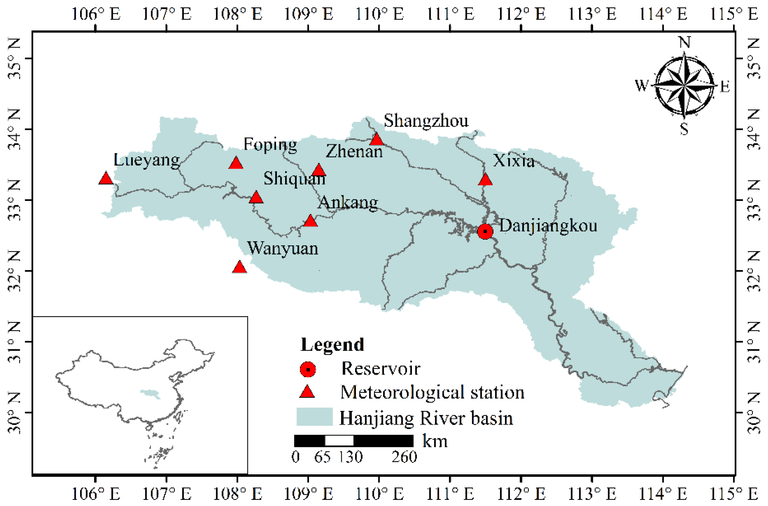
2.1. Study Area

The Hanjiang River, illustrated in Figure 1, was chosen as the case study. The river is the largest tributary of the Yangtze River. It lies between 30.28° and 34.5° N and 106.42° and 114.55° E, with a mainstream length of 1577 km and a total drainage area of 159,000 km². It originates from the southern Qin Mountain, flows through the Shanxi and Hubei provinces and converges into the Yangtze River in Wuhan. Characterized by a subtropical monsoon climate and annual precipitation of between 700 and 1100 mm, this basin has abundant water resources; 75% of the total annual precipitation occurs in the flood season (June to September). During the flood season, the sudden rainstorms in early summer and persistent rainfalls in autumn typically induce large-scale flooding [25]. For water resource regulation, a key water conservancy project named the Danjiangkou Reservoir was built in the middle of the Hanjiang River Basin. It not only serves as a source for the Middle Route of the South-to-North Water Diversion Project (MSWDP) but also plays an important role in China’s One Belt, One Road construction. Therefore, the sub-basin over Danjiangkou Reservoir is a useful candidate for conducting our proposed approach (in Section 3).

The Danjiangkou Reservoir has eased chronic water shortages in several of China’s provinces and urban cities, including the capital, Beijing. An official water diversion diagram developed by the Ministry of Water Resources of China is used for guidance of the water diversion. As shown in Figure 2, it defines a pre-set water diversion value. For example, if the reservoir water level at the initial time of the water diversion is in Region 3 (in Figure 2), the ideal water diversion flow should be 300 m³/s. Apart from water diversion, the Danjiangkou Reservoir also works as a hydropower source. Water supply and hydropower consist of the main positive purposes of the Danjiangkou Reservoir; these two objectives compete with each other, as part of the reservoir water release is redirected for water diversion instead of power generation. The basic reservoir parameters are listed in

Table 1. Characteristic parameters of the Danjiangkou Reservoir.

Characteristic	Unit	Value
Flood limited water level (FLWL)	m	160.0/163.5
Normal pool level	m	170.0
Crest elevation	m	176.6
Storage capacity for flood control	billion m3	11.44/11.00
Total storage capacity	billion m3	33.91
Guaranteed hydropower capacity	MW	247
Installed hydropower capacity	MW	900

Note: FLWL has two different values for the summer and autumn flood seasons, respectively.

.

2.2. Data Collection

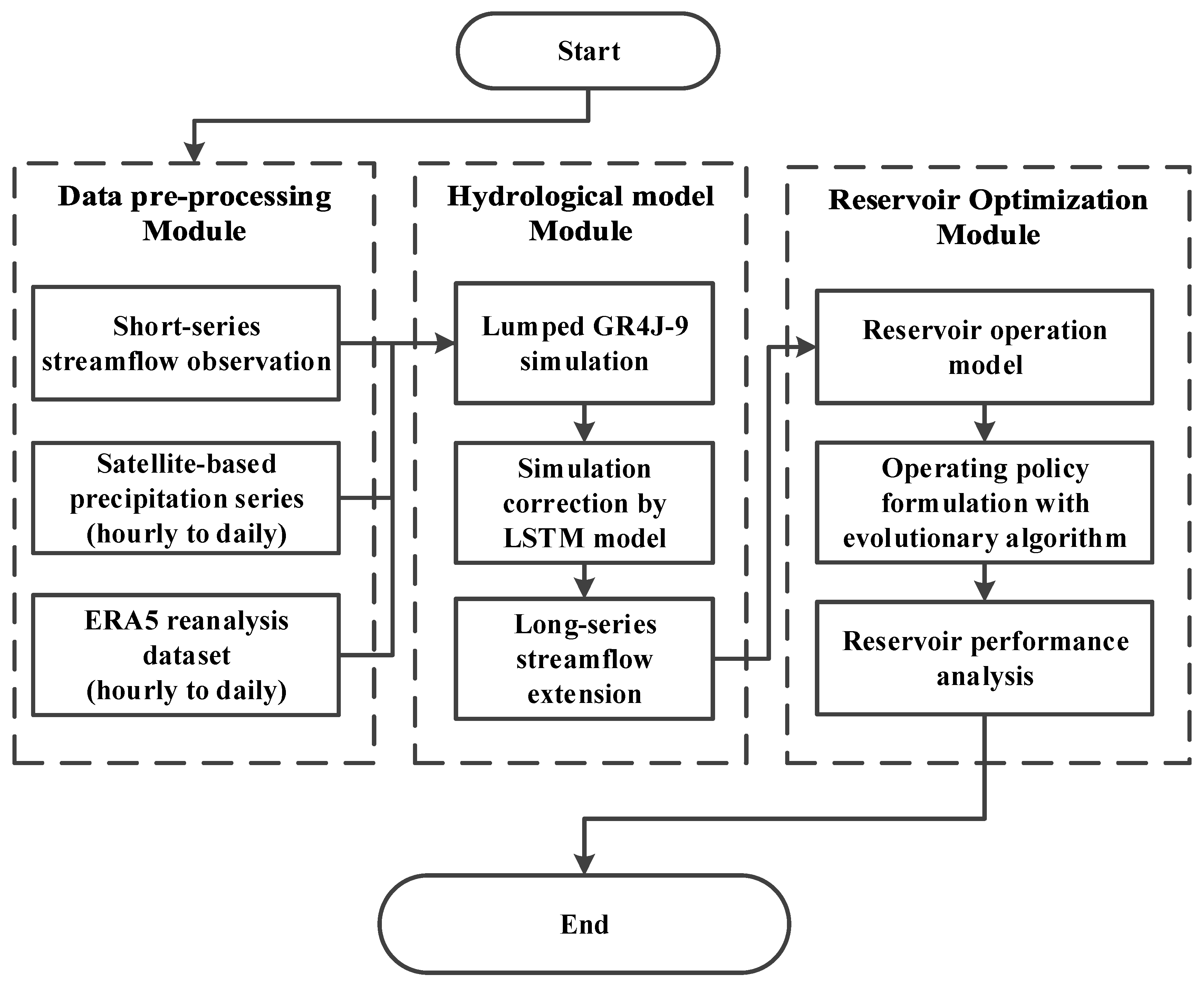
Three kinds of datasets (i.e., satellite-based observation, atmospheric reanalysis, and short-series streamflow) were collected and used in this study. The GPM Core Observatory is equipped with the first space-borne Ku/Ka-band dual-frequency radar and a multi-channel microwave imager, which improves the monitoring ability of light and solid precipitation. Since the first release of Integrated multi-satellite retrievals for GPM (IMERG) products in 2015, it has undergone many improvements, and the latest version (V06B) has been retrospectively processed, including TRMM-era data since June 2000. Due to the infusion of the Global Precipitation Climatology Centre (GPCC) rain gauge data, the final operation of IMERG provides a more accurate estimation and was therefore adopted in this study.

ERA5 was used as another meteorological product, which is a global atmospheric reanalysis dataset developed by ECMWF. ERA5 data are generated by the combination of model simulations and observations using physics laws, which are based on data assimilation by the Integrated Forecasting System (IFS Cy31r2). This assimilation system includes a four-dimensional variational (4D-Var) analysis method and considers the exact time of observation and model evolution in the assimilation window to estimate the deviation between observations and select high-quality data from poor data. The hourly output resolution is 0.25° × 0.25°, which offers a more sophisticated simulation of weather processes. The hourly near-surface air temperature, dew point temperature (T_dew), and wind speed from the ERA5 dataset were considered. All the sub-daily satellite/reanalysis data covering 2002–2019 were aggregated into a daily scale.

As the boundary of the upper and mid-lower reaches of the Hanjiang River Basin, the short-series inflow of the Danjiangkou Reservoir was selected to calibrate the parameters of the hydrological model. Observed streamflow data spanning 2003–2007 were obtained from the Yangtze River Water Conservancy Commission.

3. Methodology

A flowchart of the framework module is presented in Figure 3, which is further elaborated in the following sections. It is worth mentioning that our proposed framework can be used in hydrological simulation rather than forecasting.

3.1. Hydrological Model

The modèle du Génie Rural à 9 paramètres Journalier (GR4J-9) hydrological model was used to initially simulate the hydrology of the upper Hanjiang River watershed. The GR4J-9 model is a daily lumped nine-parameter rainfall-runoff model that integrates a traditional GR4J (five-parameter version) hydrological model with the CemaNeige snowfall accumulation and snowmelt module (which occupies four parameters). The GR4J-9 model belongs to the family of soil moisture accounting models that route runoff through two interconnected reservoirs (i.e., production and routing reservoirs) and two-unit hydrographs. It has several main parameters: the maximum capacity of the production reservoir, the groundwater exchange coefficient, the 1-day maximum retention capacity of the routing reservoir, and the time base of the unit hydrograph. This model has been tested in a large sample of catchments and has shown competitive performance compared to more complex models with more parameters [26,27]. Yang et al. [28] showed that the performance of GR4J is more stable than other models (i.e., WASMOD, HBV, and XAJ) in a changing climate. They also set the fixed coefficient of percolation leakage as a free parameter to better fit the study area and calibrated it for the objective watershed. The potential evaporation in the GR4J-9 model is obtained from the temperature-based Oudin method [29].

The observed daily precipitation (P), maximum and minimum temperature (T_max and T_min, respectively) and flow discharge were fed to calibrate and validate the GR4J-9 model for the experimental watershed. We optimized the parameters of the hydrological model using the Shuffled Complex Evolution (SCE-UA) method developed at the University of Arizona [30]. The SCE-UA method integrates the advantages of several effective global optimization concepts and employs both deterministic search strategies and random schemes to achieve an effective search ability.

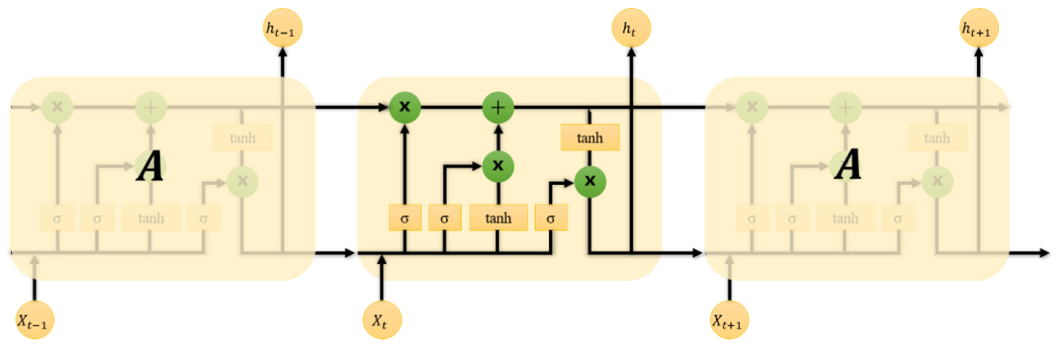
3.2. Long Short-Term Memory (LSTM) for Streamflow Simulation

3.2.1. LSTM Model

An LSTM model is a specific kind of RNN designed to overcome the drawbacks caused by a vanishing gradient or exploding in the process of training the RNN using backpropagation through time (BPTT) [31,32]. It sets up a dedicated memory cell that stores information over long periods, potentially making it an ideal candidate for modeling dynamic systems such as watersheds. An unfolded computational graph, as depicted in Figure 4, can reveal the working principle of the LSTM method. One LSTM unit is composed of an input gate, a forget gate, a memory cell and an output gate. The input gate decides which new value regulated by the memory cell will be updated in the cell state, and the forget gate controls the information to remove or retain in the cell state. A general memory block of an LSTM structure can be described by the following equations:

$$\begin{array}{c}C(t+1)=\sigma [w_{f}X(t+1)+W_{f}H(t)+b_f]\otimes C(t)+\sigma [w_{i}X(t+1)+\\ W_{i}H(t)+b_i]\otimes \tanh [w_{c}X(t+1)+W_{c}H(t)+b_c]\end{array}$$

(1)

$$H(t+1)=\sigma [w_{o}X(t+1)+W_{o}H(t)+b_o]\otimes \tanh [C(t+1)]$$

(2)

where C(t + 1) and C(t) are the cell state at time t + 1 and t, respectively; X(t + 1) and H(t + 1) are the network input and the recurrent input at time t + 1, respectively. At the initial time step, both the cell and hidden states are initialized as a vector of zeros. w and W are the weights of the link between gates and layers, respectively; b_i, b_f, b_c, and b_o are learnable bias parameters for each gate; $\sigma [\cdot ]$ is the sigmoid function and tanh$[\cdot ]$ is the hyperbolic tangent function; both are activation functions with objective values ranging from 0 to 1.

In this study, the two hyperparameters (the initial learning rate and the number of hidden nodes) diversely affecting LSTM model performance needed to be determined. A larger number of hidden neurons lead to a fully trained model, which may overfit the data; conversely, a small number of hidden neurons may cause randomness with high bias. A more detailed process of hyper-parameter tuning is described in Section 4.2. For simplicity, we chose a three-layer LSTM network as the fully connected structure, which consists of one input layer, one hidden layer, and one output layer. Preliminary investigations found that LSTMs with one single hidden layer are capable of simulating streamflow in Hanjiang River Basin [33]. The BPTT algorithm [34] was used to train the LSTM model and the adaptive moment estimation (ADAM) algorithm [35] was employed as the learning rate method. Finally, the mean square error was treated as the loss index. The general model implementation can be accessed from the Statistics and Machine Learning Toolbox of the MATLAB software (website: https://ww2.mathworks.cn/products/statistics.html# machine-learning, accessed on 22 March 2021) [36].

3.2.2. Input Variable Selection (IVS)

The appropriate determination of inputs substantially influences the development of the LSTM model [37]. For streamflow simulation, a dataset of candidate inputs typically covers observed predictors (e.g., initial basin conditions or climate elements) as well as lagged streamflow observations. A wide array of potentially hydrological components can be fed into the model; however, many may only add redundancy or a high level of noise into the model. Furthermore, some candidate inputs (e.g., long-lagged temporal data) may add little or no value to the rainfall–runoff model. To this end, the idea of input variable selection (IVS) [38] is introduced.

A tree-based IVS method developed by Galelli and Castelletti [39] was implemented to identify the optimal input combination. The extremely random tree (extra-tree) method is a non-parametric tree regression approach that partitions the input space into mutually exclusive regions on a predefined principle of splitting nodes [40]. In this particular structure, the extra-tree can rank the importance of the input variables by scoring each input variable by evaluation of the relative variance reduction. It adopts a goodness-of-fit criterion of the coefficient of determination (R²) to systematically select the most significant and non-redundant input space, which was found to consistently indicate the optimum LSTM structure in water resource modeling applications [41].

We used basin-averaged daily mean air temperature, precipitation, wind speed, relative humidity (RH), and the simulated daily discharge (corresponding to the observed reservoir inflow) from the simulations of the GR4J-9 model as the candidate inputs of the LSTM, and used observed daily discharge as the response output. Considering a typical e-folding time scale (recession time) of streamflow, we set the time lag at 4 days.

3.3. Simulation Performance Assessment

To ensure that the trained simulation model did not contain known or detectable defects and could be used on any unseen data, a comprehensive assessment was performed considering different aspects of the modeled simulation flow. Specifically, the Kling–Gupta efficiency (KGE) index was selected to describe the statistical accuracy of the hydrological models, and the objective function was to maximize the KGE value during the calibration period.

$$KGE=1-\sqrt{{(r-1)}^2+{(\alpha -1)}^2+{(\beta -1)}^2}$$

(3)

where r refers to Pearson’s linear correlation coefficient between the observation and the simulations, and $\alpha$ ($\beta$) indicates the ratio of standard deviations (mean value) of the observed and simulated streamflow. KGE varies ($-\infty$, 1]; a value closer to 1 represents a better simulation.

As shown by previous studies [42,43,44], another metric (mean relative absolute error (MRAE)) can be coupled with KGE to evaluate the overall deterministic performance.

$$MRAE=\frac{1}{T}{\displaystyle \sum _{t=1}^T\frac{|y_o^t-y_s^t|}{y_o^t}}$$

(4)

where MRAE varies [0,$\infty )$ with a perfect fit at MRAE = 0.

3.4. Policy Optimization for Reservoir Operation

3.4.1. Operation Model

As mentioned in Section 2.1, water supply and power generation are the two main yet conflicting objectives of the Danjiangkou Reservoir. Their mathematical formulations can be expressed by Equations (5) and (6).

$$W={\displaystyle \sum _{t=1}^T{Q}_t^d}\cdot \Delta t$$

(5)

$$E={\displaystyle \sum _{t=1}^T{N}_t}\cdot \Delta t,N_t=k\cdot Q_t^P\cdot H_t$$

(6)

where W and E are water supply yield (m³) and power generation (kW·h) per year, respectively; N_t is the power output at time t (kW); $Q_t^d$ and $Q_t^P$ are water diversion flow and release discharge for power generation at time t (m³/s), respectively; k is hydropower generation efficiency; H_t is the average water head at time t (m); $\Delta t$ is the time step (s); and T is the total number of operational periods.

The reservoir operation model obeys some physical constraints, which were outlined by He et al. [45]. The mathematical equations of these constraints are omitted for the sake of brevity.

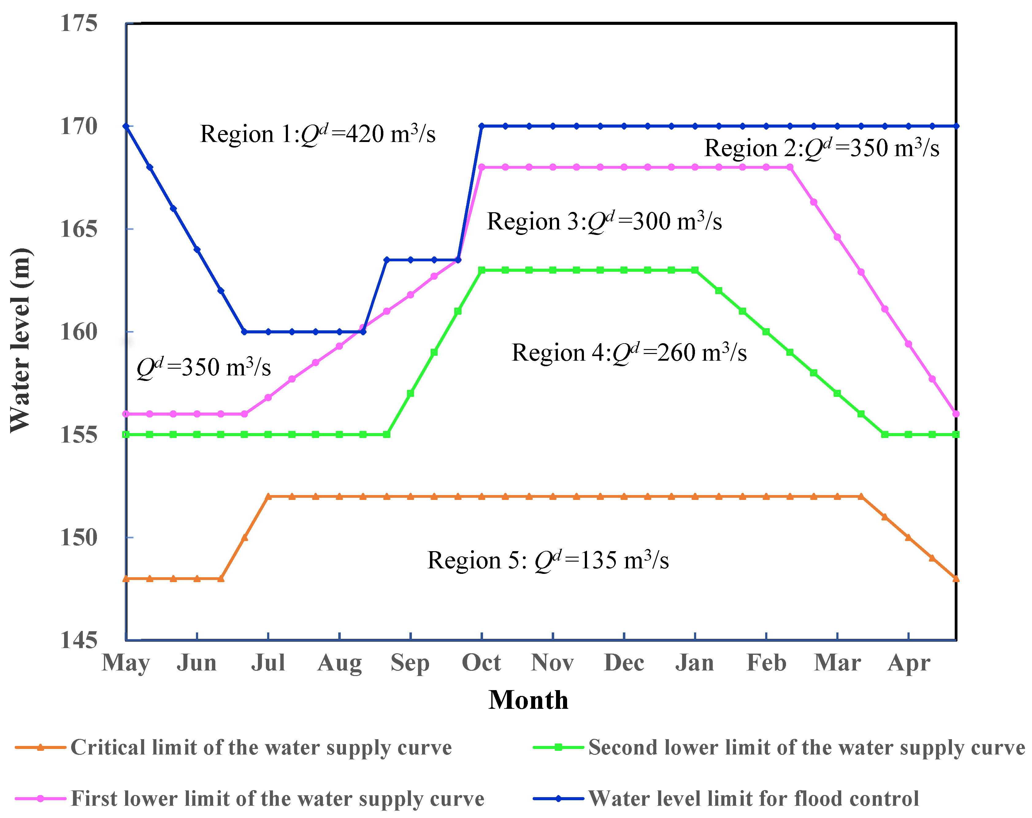
3.4.2. Operating Strategy of Reservoir Release

The optimal reservoir operation determines the reservoir release sequence $Q_t^{out}$ during the whole operating period for the maximization of W and E. As the optimization strategy of reservoir release involves a high-dimensional and non-linear property, Gaussian radial bias functions (RBFs) are taken as the operating policy, since they are flexible to make decisions with strong universal approximation [46,47]. In the RBFs method, $Q_t^{out}$ can be expressed in Equations (7) and (8).

$$Q_t^{out}={\displaystyle \sum _{u=1}^U{\omega }_u{\phi }_u(X_t),\hspace{1em}t\in [1,T]}$$

(7)

$${\phi }_u(X_t)=\exp [-{\displaystyle \sum _{m=1}^M\frac{{({(X_t)}_m-c_{m,u})}^2}{b_u}}]\hspace{1em}{c}_{m,u}\in [-1,1],b_{m,u}\in (0,1]$$

(8)

where U is the total number of RBFs $\phi (\cdot )$; ${\omega }_u$ is the weight of the uth RBF, the sum of all weights is 1, e.g., ${\displaystyle \sum _{u=1}^U{\omega }_u}=1$. M is the number of input variables of X_t; and c_m,u and b_u are the mth-dimensional center and radius of the uth RBF, respectively. For an individual reservoir, X_t usually consists of three variables, namely time at time t, current reservoir storage (V_t) and reservoir inflow information ($Q_t^{in}$) [48]; thus, M was set to 3. Moreover, each RBF can be regarded as one pattern of decision-making in reservoir operation based on X_t and, ultimately, decision-making is determined by the combination of four patterns (i.e., U is 4) as suggested by Yang et al. [48].

Consequently, there were 20 parameters to be calibrated for the sum of the RBFs. We optimized the parameter combination based on the parameterization–simulation–optimization (PSO) framework using the non-dominated sorting genetic algorithm II (NSGA-II). To converge the Pareto front, the evolutionary NSGA-II algorithm adopts the fast non-dominated sorting and crowding distance strategies. The experimental setup of NSGA-II was: population size = 100, generation number = 1000, crossover probability = 0.9, and mutation probability = 0.1.

4. Results and Discussion

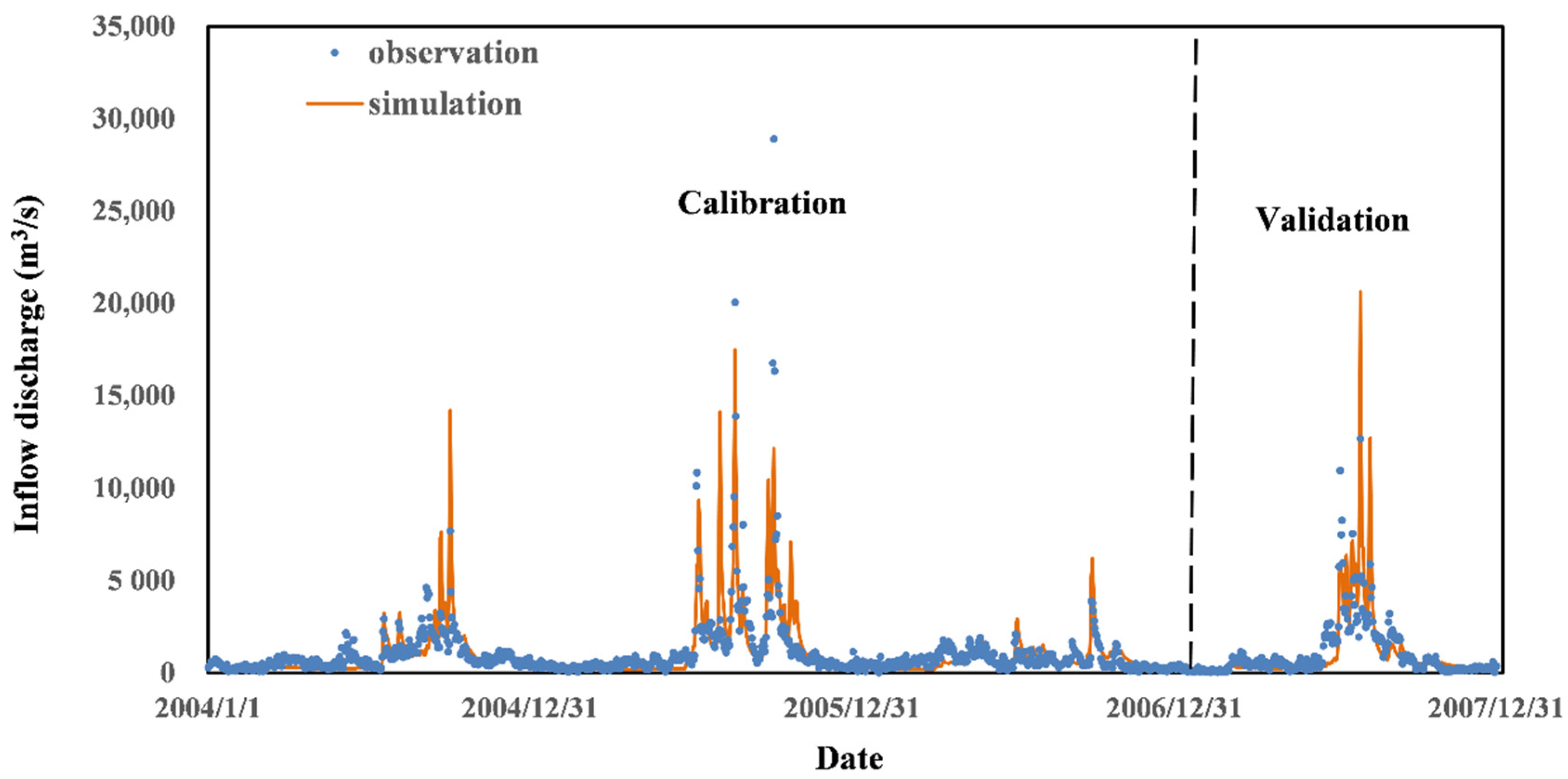
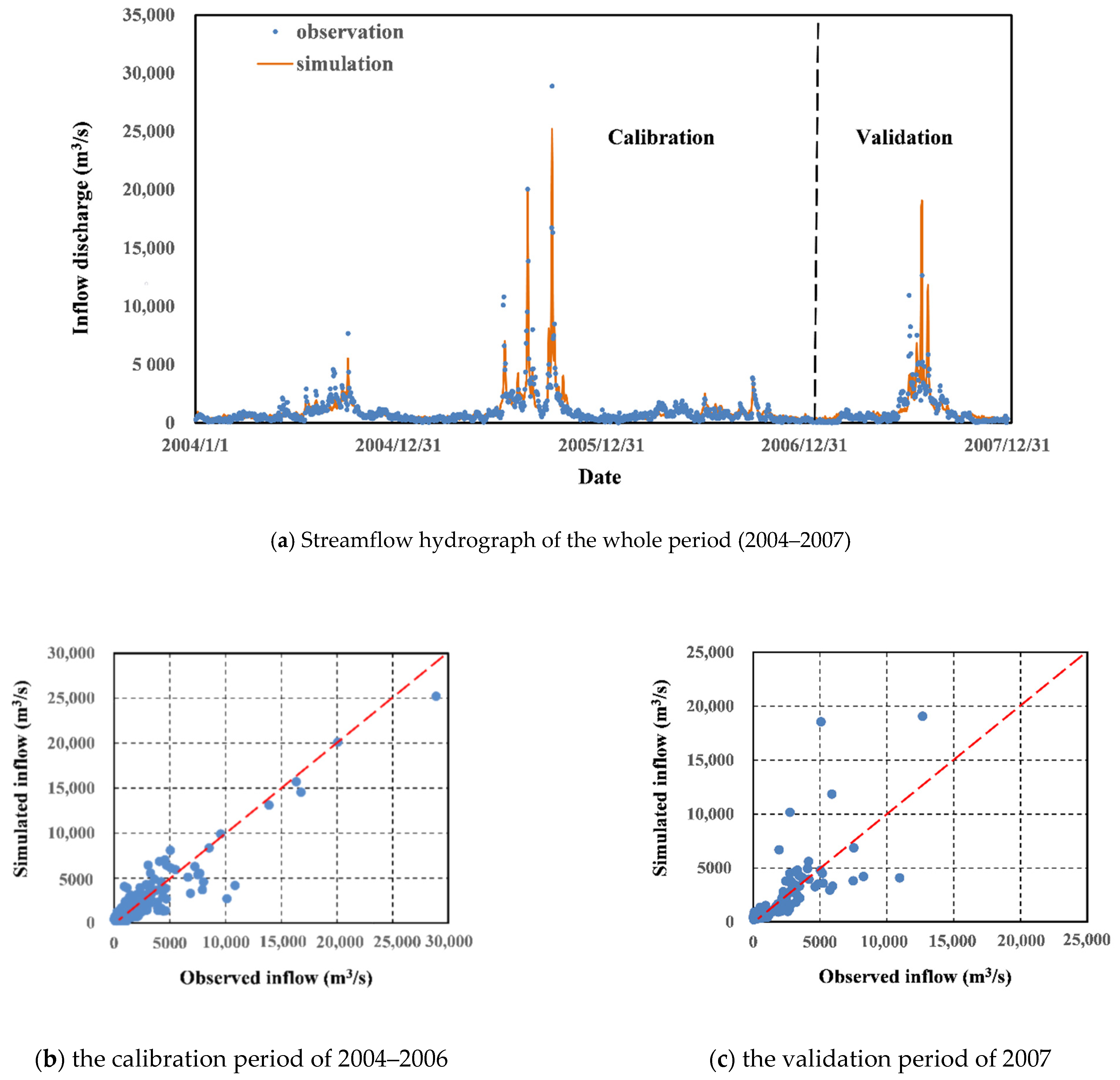
4.1. Initial Simulation of the GR4J-9 Model

We first calibrated and validated the GR4J-9 model using observed reservoir inflow during 2003–2007. With the first year serving as the warm-up period, the KGE values of the calibration (2004–2006, three years) and validation periods (2007, one year) were 0.76 and 0.54, respectively; the MRAE values were 0.56 and 0.73, respectively. As recommended by previous studies, the model performance is judged to be satisfactory for flow simulations if the daily KGE is greater than 0.5 and the MRAE is less than 0.85 for watershed-scale models [2,49].

Figure 5 depicts the simulation results for reservoir inflow. It shows that the GR4J-9 model could fit the inflow hydrograph of the calibration well, especially for a low inflow regime. However, it achieved a relatively low KGE value in the validation period, with a serious underestimation. In detail, the GR4J-9 model cannot capture the peak discharge of 28,900 m³/s, and instead, gives a lower value of 12,461 m³/s. Similar results were also found at other different times, which were caused by several aspects. From the view of model inputs, the basin-averaged daily precipitation still has a relatively low resolution compared to actual precipitation observations. From the view of model structure, GR4J-9 has a simple structure with nine model parameters. Although it has superior performance compared to distributed models in the ungauged basin (the latter need more sub-basin observations to calibrate parameters), it inevitably leads to a model error where the simple structure assumption fails to cater to the actual hydrological condition. Therefore, it is necessary to develop a state-of-the-art technique to further improve streamflow accuracy.

4.2. LSTM Performance

As stated in Section 3.2.2, we fed the GR4J-9 model output into the advanced LSTM model, which also included wind speed and RH. To derive RH data for LSTM inputs, we used the daily dew point temperature (T_dew) and daily mean temperature (T_mean) from ERA5. The actual vapor pressure (e) and saturated vapor pressure ($e_{\mathrm{sa}})$ were derived using the Clausius–Clapeyron equation. The determined input variables were normalized to eliminate the influence of magnitude, thereby improving the accuracy and efficiency of network learning.

As anticipated, the tree-based IVS algorithm could score and rank input variables in terms of their relevance to the output. To ensure a reliable ranking result, the experiment was cross-validated multiple times with different shuffled datasets, and the inputs were sorted in decreasing order. The score results of the IVS run are presented in

Table 2. The top 11 input ranking results for the upper Hanjiang River Basin dataset.

Variable	${\mathit{Q}}_{\mathit{t}}^{\mathit{s}\mathit{i}\mathit{m}}$	${\mathit{Q}}_{\mathit{t}-1}^{\mathit{s}\mathit{i}\mathit{m}}$	${\mathit{P}}_{\mathit{t}-1}^{}$	${\mathit{Q}}_{\mathit{t}-2}^{\mathit{s}\mathit{i}\mathit{m}}$	${\mathit{P}}_{\mathit{t}}^{}$	$\mathit{R}{\mathit{H}}_{\mathit{t}}^{}$	$\mathit{W}{\mathit{D}}_{\mathit{t}}^{}$	${\mathit{P}}_{\mathit{t}-2}^{}$	${\mathit{Q}}_{\mathit{t}-3}^{\mathit{s}\mathit{i}\mathit{m}}$	${\mathit{Q}}_{\mathit{t}-4}^{\mathit{s}\mathit{i}\mathit{m}}$	${\mathit{P}}_{\mathit{t}-3}^{}$
Score (%)	23.84	16.14	13.54	8.38	6.55	5.27	5.03	4.06	2.31	2.01	1.34
Ranking	1	2	3	4	5	6	7	8	9	11	12

, which illustrates the importance of each selected variable. This tree-based method can make sense for the ex-post physical interpretation of the cause–effect relationships captured by the model. For the upper Hanjiang River Basin, the simulated flow at time t by the GR4J-9 model ($Q_t^{sim}$), precipitation ($P_t^{}$), antecedent simulated flow and precipitation with 1- or 2-time lag ($Q_{t-1}^{sim}$, $Q_{t-2}^{sim}$ and $P_{t-1}^{}$, respectively) were the top five most important variables (about 68% of the ensemble total score), followed by relative humidity and wind speed at time t (i.e., RH_t and WD_t, respectively). Except for the simulated streamflow element, which was highly related to the observed inflow, we found that $P_{t-1}^{}$ and $P_t^{}$ ranked in the top positions, with relative scores of 13% and 6%, respectively. This may be due to the hydraulic characteristics of this large catchment, which is drained by base flow with a long period of concentration. The basin-averaged RH and wind speed are less important, but not negligible.

Finally, antecedent simulated flow with 1–4 time lags ($Q_t^{sim}$,$Q_{t-1}^{sim}$,$Q_{t-2}^{sim}$,$Q_{t-3}^{sim}$, and $Q_{t-4}^{sim}$, respectively), antecedent simulated flow with 1–3 time lags ($P_t^{}$,$P_{t-1}^{}$,$P_{t-2}^{}$ and $P_{t-3}^{}$, respectively), RH_t and WD_t consisted of 11 inputs for the LSTM machine learning model. With a hidden layer of 64 neurons and an initial learning rate of 0.1 (identified by the trial-and-error method), the LSTM-based model could substantially improve the accuracy of the streamflow simulation compared to the GR4J-9 benchmark model. The daily streamflow trajectories are shown in Figure 6a. The model achieved a high KGE value of 0.87 and MRAE of 0.56 for the daily discharge in the calibration period; additionally, the KGE was 0.68 and the MRAE value was 0.71 in the validation period. The results demonstrated that this method can competently ameliorate the hydrological data scarcity. Compared to the benchmark GR4J-9 model, the LSTM model uses related hydrological variables (i.e., RH and wind speed) as driving inputs to improve streamflow accuracy. Compared to physically distributed hydrological models, which have limited applications in basins with short-series datasets due to the complex characteristics [50], the LSTM model can sufficiently use remote sensing data and has the features of easy-to-use and highly efficient. However, the LSTM model displayed serious overestimation behavior in the validation period. This is due to the LSTM model being overly reliant on the calibrated data without exception. Figure 6a,b show that the streamflow simulations corrected by the LSTM model are closer to the peak discharge in the calibration. This overfitting performance was unfortunately carried into the validation period, which caused the LSTM model to provide a relatively high value for streamflow discharge under low flow regimes. In general, the LSTM model has room for improvement, but this does not hinder its application value.

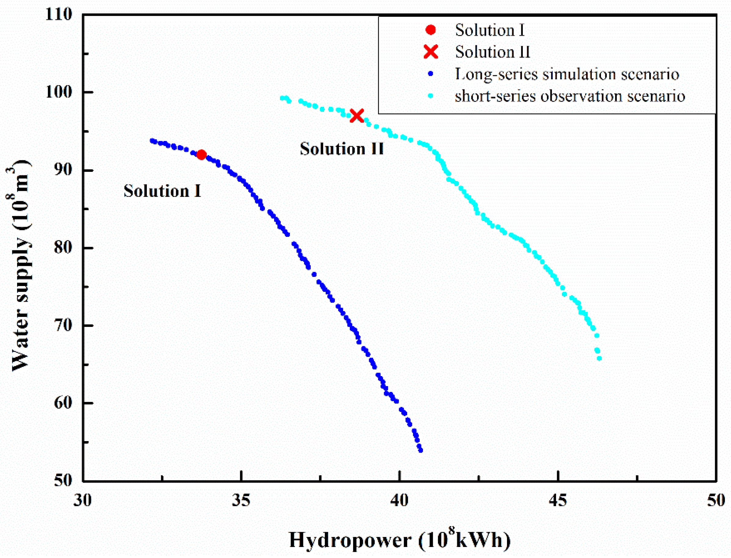
4.3. Potential Application in Reservoir Management

We acquired a long-series daily streamflow simulation from the period of 2008–2019 by feeding the remote sensing data into the calibrated LSTM model. We could formulate more scientific strategies for basins with hydrological data scarcity. Using the medium- and long-term management of the Danjiangkou Reservoir operation as an example, we aimed to improve hydropower benefits and water supply yield and balance them as much as possible. Before performing the NSGA-II reservoir optimization method, daily scale simulated streamflow was converted into 10-day average runoff.

The optimization results of W and E by NSGA-II are presented in Figure 7, and the operation results merely based on short-series observation (2003–2007) are also provided for further comparison. Both of the Pareto fronts under different scenarios are widely and evenly distributed between the two conflicting objectives. Considering the pursuit of maximum economic profit (official electricity price: 0.21 RMB/kWh; water price for the MSWTP project: 0.13 RMB/m³), the final two optimal operating rules were chosen for promising economic prospect, namely Solution I under long-series simulated scenario of 2003–2019 and Solution II under short-series observed scenario of 2003–2007 (in Figure 7).

With these two optimal operating rules guiding reservoir operation during the period of 2003–2019, their objective results are summarized in

Table 3. Objective results of two optimal rules in different periods.

Operating Rule	Different Season	Observation Period (2003–2007)			Whole Period (2003–2019)
		W (108 m3)	E (108 kWh)	H (108 RMB)	W (108 m3)	E (108 kWh)	H (108 RMB)
Solution I	flood	34.25	14.68	7.54	32.16	13.67	7.05
	non-flood	64.72	22.76	13.19	59.83	20.08	12.00
	annual	98.97	37.44	20.73	91.99	33.75	19.05
Solution II	wet	33.77	15.20	7.58	31.24	13.62	6.92
	dry	63.48	23.62	13.21	58.21	20.85	11.95
	annual	97.25	38.82	20.79	89.45	34.47	18.86

Note: W = water supply, E = hydropower, and H = economic profit.

. It can be inferred from water supply, hydropower, and economic profit (W, E, and H, respectively) that Solution I prefers a higher value of W than Solution II, no matter whether in the observation period or in the whole period when decision-makers want to pursue more economic profit. As shown in Table 3, while the performance of Solution I (obtained through LSTM-based streamflow simulation) is similar to that of Solution II, it provides decision-makers with another viable operating way that requires more real observational data to verify.

5. Conclusions

Hydro-meteorological data scarcity impairs hydrological simulation, manifesting a pressing need to develop an alternative scheme in this field. Satellite-based and atmospheric reanalysis estimation may provide feasible access to reproduce the hydrological recycle process and may have potential value. To this end, this paper proposed a novel method to integrate open-source remote sensing data and ML-based inversion techniques for hydrology. Furthermore, we applied it in reservoir management. According to the results, we reached the following conclusions:

(1)

Driven by the synthetic data generated by a lumped hydrological GR4J model, satellite-based data and ERA5 could overcome the limitation of historical observation scarcity. With a KGE value of 0.54 in the validation period for the upper Hanjiang River Basin, the traditional lumped hydrological model can be applied to the ungauged basins but there is still room for improvement.

(2)

Compared to the traditional GR4J model, the ML-based data-driven model showed its superior performance in capturing the long-series time sequence using a sophisticated network structure. Along with inheriting the simulation output of the traditional hydrological model, the LSTM model can further mine the value of remote sensing data related to hydrological variables. Compared to traditional distributed hydrological models, its model structure is simple and can be highly efficient.

(3)

The LSTM-based streamflow simulation scenario can provide the basis for another scientific operation way for reservoir managers, which requires future validation of the potential value of the LSTM-based method.

Despite the outstanding performance of the developed methodology, some work remains for further exploration. First, hydrological models have different behaviors depending on the flow regimes. However, in this study, the hydro-meteorological data with a one-day timescale were fed to drive one set of hydrological models, yet the separation of flood seasons and non-flood seasons was neglected. Besides, a simpler LSTM model should be taken into consideration and compared with our proposed hybrid model for hydrological performance. Secondly, the methodology was merely applied for hydrological simulation rather than hydrological forecasts. Some products such as the Global Ensemble Forecast System (GEFS) Reforecast can be included to improve this methodology. In the future, we will explore the ML-based method with remote sensing data to verify its generalizability in more ungauged basins.

References

1. Ferreira, R.G.; da Silva, D.D.; Elesbon, A.A.A.; Fernandes-Filho, E.I.; Veloso, G.V.; Fraga, M.D.S.; Ferreira, L.B. Machine learning models for streamflow regionalization in a tropical watershed. J. Environ. Manag. 2021, 280, 111713. [Google Scholar] [CrossRef]
2. Gu, L.; Chen, J.; Yin, J.; Xu, C.Y.; Zhou, J. Responses of Precipitation and Runoff to Climate Warming and Implications for Future Drought Changes in China. Earths Future 2020, 8, 8. [Google Scholar] [CrossRef]
3. Zhou, Y.; Guo, S.; Chang, F.-J. Explore an evolutionary recurrent ANFIS for modelling multi-step-ahead flood forecasts. J. Hydrol. 2019, 570, 343–355. [Google Scholar] [CrossRef]
4. Suwal, N.; Kuriqi, A.; Huang, X.F.; Delgado, J.; Mlynski, D.; Walega, A. Environmental Flows Assessment in Nepal: The Case of Kaligandaki River. Sustainability 2020, 12, 8766. [Google Scholar] [CrossRef]
5. Yin, J.; Guo, S.; Gentine, P.; Sullivan, S.C.; Gu, L.; He, S.; Chen, J.; Liu, P. Does the Hook Structure Constrain Future Flood Intensification Under Anthropogenic Climate Warming? Water Resour. Res. 2021, 57. [Google Scholar] [CrossRef]
6. Shen, Y.; Liu, D.; Jiang, L.; Yin, J.; Nielsen, K.; Bauer-Gottwein, P.; Guo, S.; Wang, J. On the Contribution of Satellite Altimetry-Derived Water Surface Elevation to Hydrodynamic Model Calibration in the Han River. Remote Sens. 2020, 12, 4087. [Google Scholar] [CrossRef]
7. Bastola, S.; Misra, V. Evaluation of dynamically downscaled reanalysis precipitation data for hydrological application. Hydrol. Process. 2014, 28, 1989–2002. [Google Scholar] [CrossRef]
8. Weedon, G.P.; Balsamo, G.; Bellouin, N.; Gomes, S.; Best, M.J.; Viterbo, P. The WFDEI meteorological forcing data set: WATCH Forcing Data methodology applied to ERA-Interim reanalysis data. Water Resour. Res. 2014, 50, 7505–7514. [Google Scholar] [CrossRef] [Green Version]
9. Guan, X.X.; Zhang, J.Y.; Yang, Q.L.; Tang, X.P.; Liu, C.S.; Jin, J.L.; Liu, Y.; Bao, Z.X.; Wang, G.Q. Evaluation of Precipitation Products by Using Multiple Hydrological Models over the Upper Yellow River Basin, China. Remote Sens. 2020, 12, 4023. [Google Scholar] [CrossRef]
10. Bastola, S.; François, D. Temporal extension of meteorological records for hydrological modelling of Lake Chad Basin (Africa) using satellite rainfall data and reanalysis datasets. Meteorol. Appl. 2012, 19, 54–70. [Google Scholar] [CrossRef]
11. Mazzoleni, M.; Alfonso, L.; Solomatine, D. Influence of spatial distribution of sensors and observation accuracy on the assimilation of distributed streamflow data in hydrological modelling. Hydrol. Sci. J. 2017, 62, 389–407. [Google Scholar] [CrossRef]
12. Kuriqi, A.; Ali, R.; Pham, Q.B.; Gambini, J.M.; Gupta, V.; Malik, A.; Linh, N.T.T.; Joshi, Y.; Anh, D.T.; Nam, V.T.; et al. Seasonality shift and streamflow flow variability trends in central India. Acta Geophys. 2020, 68, 1461–1475. [Google Scholar] [CrossRef]
13. Chang, L.C.; Chang, F.J.; Hsu, H.C. Real-Time Reservoir Operation for Flood Control Using Artificial Intelligent Techniques. Int. J. Nonlin. Sci. Num. 2010, 11, 887–902. [Google Scholar] [CrossRef]
14. Sadler, J.M.; Goodall, J.L.; Morsy, M.M.; Spencer, K. Modeling urban coastal flood severity from crowd-sourced flood reports using Poisson regression and Random Forest. J. Hydrol. 2018, 559, 43–55. [Google Scholar] [CrossRef]
15. Kopeć, A.; Trybała, P.; Głąbicki, D.; Buczyńska, A.; Owczarz, K.; Bugajska, N.; Kozińska, P.; Chojwa, M.; Gattner, A. Application of Remote Sensing, GIS and Machine Learning with Geographically Weighted Regression in Assessing the Impact of Hard Coal Mining on the Natural Environment. Sustainability 2020, 12, 9338. [Google Scholar] [CrossRef]
16. Manfreda, S.; Samela, C. A digital elevation model based method for a rapid estimation of flood inundation depth. J. Flood Risk Manag. 2019, 12. [Google Scholar] [CrossRef] [Green Version]
17. Solomatine, D.P.; Shrestha, D.L. A novel method to estimate model uncertainty using machine learning techniques. Water Resour. Res. 2009, 45. [Google Scholar] [CrossRef]
18. Adnan, R.M.; Zounemat-Kermani, M.; Kuriqi, A.; Kisi, O. Machine Learning Method in Prediction Streamflow Considering Periodicity Component. In Intelligent Data Analytics for Decision-Support Systems in Hazard Mitigation: Theory and Practice of Hazard Mitigation; Deo, R.C., Samui, P., Kisi, O., Yaseen, Z.M., Eds.; Springer: Singapore, 2021; pp. 383–403. [Google Scholar] [CrossRef]
19. Zhang, D.; Peng, Q.; Lin, J.; Wang, D.; Liu, X.; Zhuang, J. Simulating Reservoir Operation Using a Recurrent Neural Network Algorithm. Water 2019, 11, 865. [Google Scholar] [CrossRef] [Green Version]
20. Misra, S.; Sarkar, S.; Mitra, P. Statistical downscaling of precipitation using long short-term memory recurrent neural networks. Theor. Appl. Climatol. 2017, 134, 1179–1196. [Google Scholar] [CrossRef]
21. Nourani, V.; Baghanam, A.H.; Adamowski, J.; Kisi, O. Applications of hybrid wavelet-Artificial Intelligence models in hydrology: A review. J. Hydrol. 2014, 514, 358–377. [Google Scholar] [CrossRef]
22. Zhang, H.B.; Singh, V.P.; Bin Wang, B.; Yu, Y.H. CEREF: A hybrid data-driven model for forecasting annual streamflow from a socio-hydrological system. J. Hydrol. 2016, 540, 246–256. [Google Scholar] [CrossRef]
23. Cheng, M.; Fang, F.; Kinouchi, T.; Navon, I.M.; Pain, C.C. Long lead-time daily and monthly streamflow forecasting using machine learning methods. J. Hydrol. 2020, 590, 125376. [Google Scholar] [CrossRef]
24. Fu, M.; Fan, T.; Ding, Z.a.; Salih, S.Q.; Al-Ansari, N.; Yaseen, Z.M. Deep Learning Data-Intelligence Model Based on Adjusted Forecasting Window Scale: Application in Daily Streamflow Simulation. IEEE Access 2020, 8, 32632–32651. [Google Scholar] [CrossRef]
25. He, S.K.; Guo, S.L.; Yang, G.; Chen, K.B.; Liu, D.D.; Zhou, Y.L. Optimizing Operation Rules of Cascade Reservoirs for Adapting Climate Change. Water Resour. Manag. 2020, 34, 101–120. [Google Scholar] [CrossRef]
26. Kunnath-Poovakka, A.; Eldho, T.I. A comparative study of conceptual rainfall-runoff models GR4J, AWBM and Sacramento at catchments in the upper Godavari river basin, India. J. Earth Syst. Sci. 2019, 128, 33. [Google Scholar] [CrossRef] [Green Version]
27. Edijatno; Nascimento, N.D.; Yang, X.L.; Makhlouf, Z.; Michel, C. GR3J: A daily watershed model with three free parameters. Hydrol. Sci. J. 1999, 44, 263–277. [Google Scholar]
28. Yang, W.S.; Chen, H.; Xu, C.Y.; Huo, R.; Chen, J.; Guo, S.L. Temporal and spatial transferabilities of hydrological models under different climates and underlying surface conditions. J. Hydrol. 2020, 591, 125276. [Google Scholar] [CrossRef]
29. Oudin, L.; Hervieu, F.; Michel, C.; Perrin, C.; Andréassian, V.; Anctil, F.; Loumagne, C. Which potential evapotranspiration input for a lumped rainfall–runoff model? J. Hydrol. 2005, 303, 290–306. [Google Scholar] [CrossRef]
30. Duan, Q.; Sorooshian, S.; Gupta, V. Effective and efficient global optimization for conceptual rainfall-runoff models. Water Resour. Res. 1992, 28, 1015–1031. [Google Scholar] [CrossRef]
31. Hochreiter, S.; Schmidhuber, J. Long short-term memory. Neural Comput. 1997, 9, 1735–1780. [Google Scholar] [CrossRef] [PubMed]
32. Bengio, Y.; Simard, P.; Frasconi, P. Learning Long-Term Dependencies with Gradient Descent Is Difficult. IEEE Trans. Neural Netw. 1994, 5, 157–166. [Google Scholar] [CrossRef]
33. Hu, Q.; Cao, S.; Yang, H.; Wang, Y.; Li, L.; Wang, L. Daily runoff predication using LSTM at the Ankang Station, Hanjing River. Prog. Geogr. 2020, 39, 636–642. [Google Scholar] [CrossRef]
34. Werbos, P.J. Backpropagation through Time-What It Does and How to Do It. Proc. IEEE 1990, 78, 1550–1560. [Google Scholar] [CrossRef] [Green Version]
35. Chang, Z.H.; Zhang, Y.; Chen, W.B. Electricity price prediction based on hybrid model of adam optimized LSTM neural network and wavelet transform. Energy 2019, 187, 115804. [Google Scholar] [CrossRef]
36. Zhou, Y.L. Real-time probabilistic forecasting of river water quality under data missing situation: Deep learning plus post-processing techniques. J. Hydrol. 2020, 589, 125164. [Google Scholar] [CrossRef]
37. Kratzert, F.; Klotz, D.; Shalev, G.; Klambauer, G.; Hochreiter, S.; Nearing, G. Towards learning universal, regional, and local hydrological behaviors via machine learning applied to large-sample datasets. Hydrol. Earth Syst. Sci. 2019, 23, 5089–5110. [Google Scholar] [CrossRef] [Green Version]
38. Humphrey, G.B.; Gibbs, M.S.; Dandy, G.C.; Maier, H.R. A hybrid approach to monthly streamflow forecasting: Integrating hydrological model outputs into a Bayesian artificial neural network. J. Hydrol. 2016, 540, 623–640. [Google Scholar] [CrossRef]
39. Galelli, S.; Castelletti, A. Tree-based iterative input variable selection for hydrological modeling. Water Resour. Res. 2013, 49, 4295–4310. [Google Scholar] [CrossRef]
40. Jaxa-Rozen, M.; Kwakkel, J. Tree-based ensemble methods for sensitivity analysis of environmental models: A performance comparison with Sobol and Morris techniques. Environ. Model. Softw. 2018, 107, 245–266. [Google Scholar] [CrossRef]
41. Li, Y.T.; Bao, T.F.; Gong, J.; Shu, X.S.; Zhang, K. The Prediction of Dam Displacement Time Series Using STL, Extra-Trees, and Stacked LSTM Neural Network. IEEE Access 2020, 8, 94440–94452. [Google Scholar] [CrossRef]
42. Gupta, H.V.; Kling, H.; Yilmaz, K.K.; Martinez, G.F. Decomposition of the mean squared error and NSE performance criteria: Implications for improving hydrological modelling. J. Hydrol. 2009, 377, 80–91. [Google Scholar] [CrossRef] [Green Version]
43. He, S.K.; Guo, S.L.; Liu, Z.J.; Yin, J.B.; Chen, K.B.; Wu, X.S. Uncertainty analysis of hydrological multi-model ensembles based on CBP-BMA method. Hydrol. Res. 2018, 49, 1636–1651. [Google Scholar] [CrossRef] [Green Version]
44. Moriasi, D.N.; Arnold, J.G.; Van Liew, M.W.; Bingner, R.L.; Harmel, R.D.; Veith, T.L. Model evaluation guidelines for systematic quantification of accuracy in watershed simulations. Trans. ASABE 2007, 50, 885–900. [Google Scholar] [CrossRef]
45. He, S.K.; Guo, S.L.; Chen, K.B.; Deng, L.L.; Liao, Z.; Xiong, F.; Yin, J.B. Optimal impoundment operation for cascade reservoirs coupling parallel dynamic programming with importance sampling and successive approximation. Adv. Water Resour. 2019, 131. [Google Scholar] [CrossRef]
46. Giuliani, M.; Castelletti, A. Is robustness really robust? How different definitions of robustness impact decision-making under climate change. Clim. Chang. 2016, 135, 409–424. [Google Scholar] [CrossRef]
47. Giudici, F.; Castelletti, A.; Giuliani, M.; Maier, H.R. An active learning approach for identifying the smallest subset of informative scenarios for robust planning under deep uncertainty. Environ. Model. Softw. 2020, 127, 104681. [Google Scholar] [CrossRef]
48. Yang, G.; Guo, S.L.; Liu, P.; Li, L.P.; Xu, C.Y. Multiobjective reservoir operating rules based on cascade reservoir input variable selection method. Water Resour. Res. 2017, 53, 3446–3463. [Google Scholar] [CrossRef]
49. Yin, J.B.; Guo, S.L.; Gu, L.; He, S.K.; Ba, H.H.; Tian, J.; Li, Q.X.; Chen, J. Projected changes of bivariate flood quantiles and estimation uncertainty based on multi-model ensembles over China. J. Hydrol. 2020, 585, 124760. [Google Scholar] [CrossRef]
50. Yang, S.; Yang, D.; Chen, J.; Santisirisomboon, J.; Lu, W.; Zhao, B. A physical process and machine learning combined hydrological model for daily streamflow simulations of large watersheds with limited observation data. J. Hydrol. 2020, 590, 125206. [Google Scholar] [CrossRef]
Figure 1. Geographic information of the Danjiangkou Reservoir in the Hanjiang River Basin.
Sustainability 13 03645 g001
Figure 2. The operation rule curves of the Danjiangkou Reservoir for water supply.
Sustainability 13 03645 g002
Figure 3. Flowchart of streamflow retrieval and its potential application value.
Sustainability 13 03645 g003
Figure 4. Architecture diagram of the long short-term memory (LSTM) model.
Sustainability 13 03645 g004
Figure 5. Simulation result of reservoir inflow by the modèle du Génie Rural à 9 paramètres Journalier (GR4J-9) model.
Sustainability 13 03645 g005
Figure 6. Simulation result of reservoir inflow by the long and short-term model (LSTM) model. (a) Inflow hydrograph in the whole period; (b) Scatter plot of the calibration period; (c) Scatter plot of the validation period.
Sustainability 13 03645 g006
Figure 7. Two sets of Pareto fronts in different streamflow scenarios.
Sustainability 13 03645 g007