
Novel Ensemble Forecasting of Streamflow Using Locally Weighted Learning Algorithm

 ,
,  ,
,  ,
,  and
and
Abstract
:1. Introduction
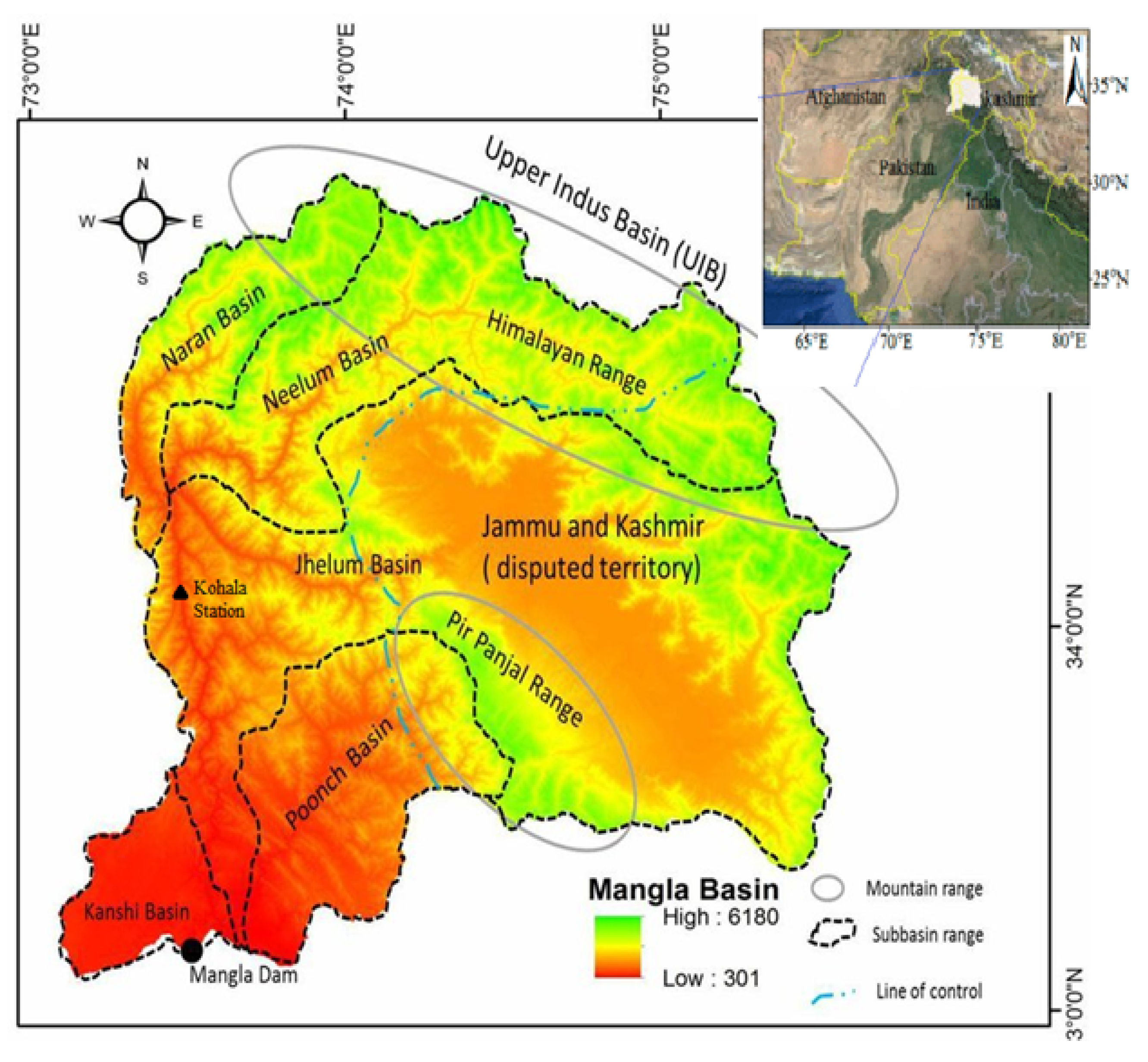
2. Case Study
3. Methods
3.1. Locally Weighted Learning (LWL) Algorithm
3.2. Bagging
3.3. Additive Regression
3.4. Random Subspace (RS)
3.5. Dagging
3.6. Rotation Forest
4. Ensemble Forecasting
- (i)
- Qt-1
- (ii)
- Qt-1, Qt-2
- (iii)
- Qt-1, Qt-2, Qt-3
- (iv)
- Qt-1, Qt-2, Qt-3, MN
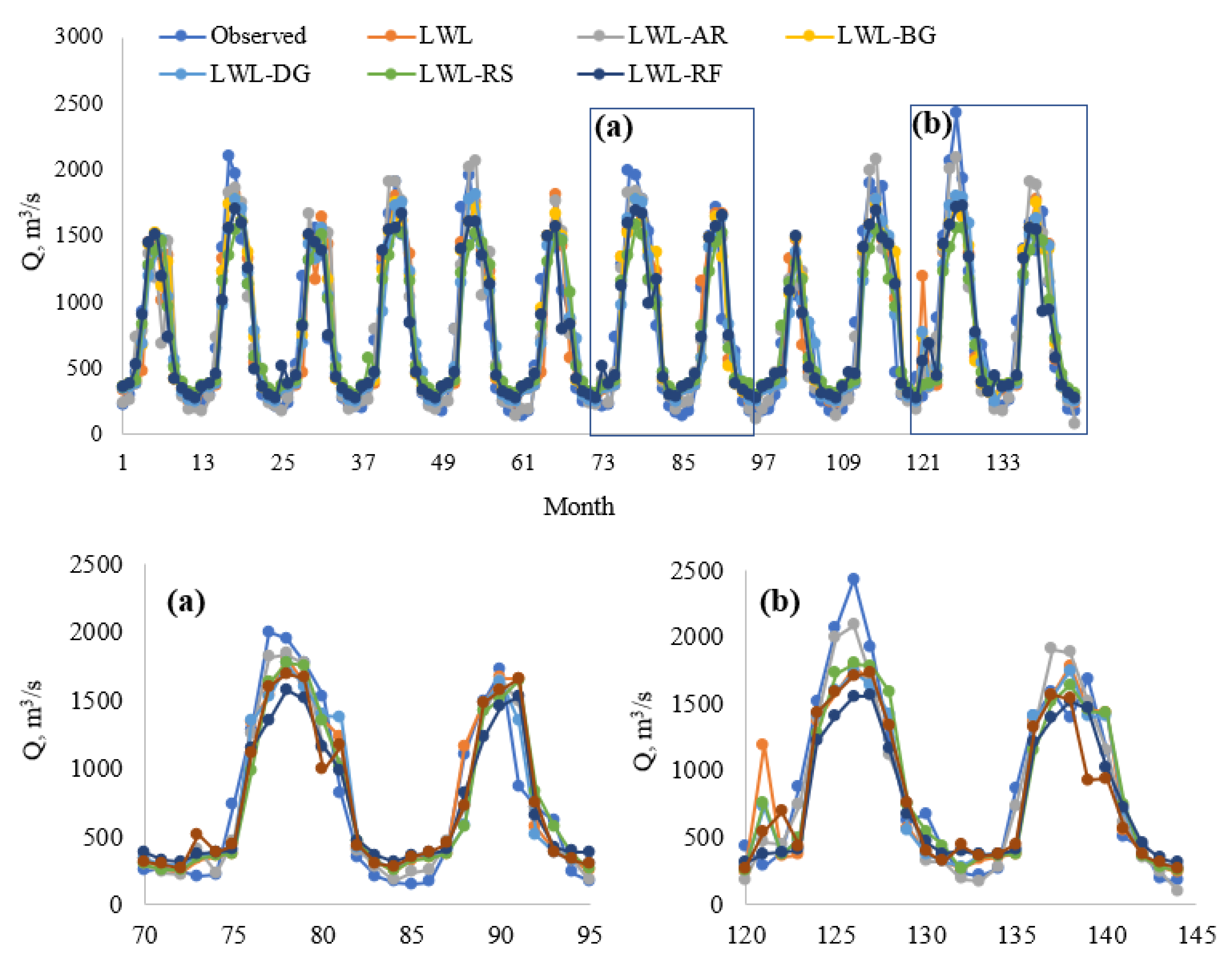
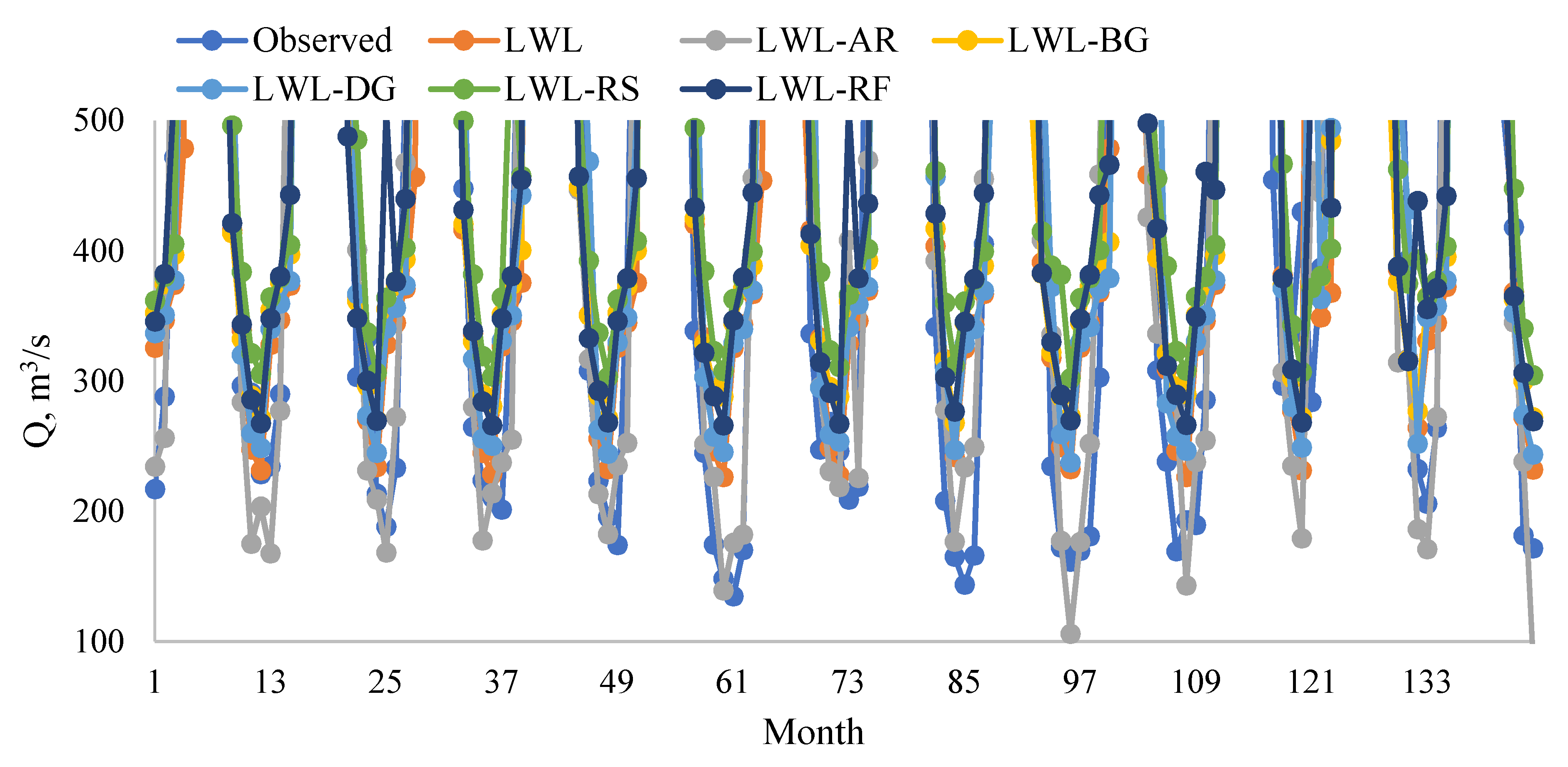
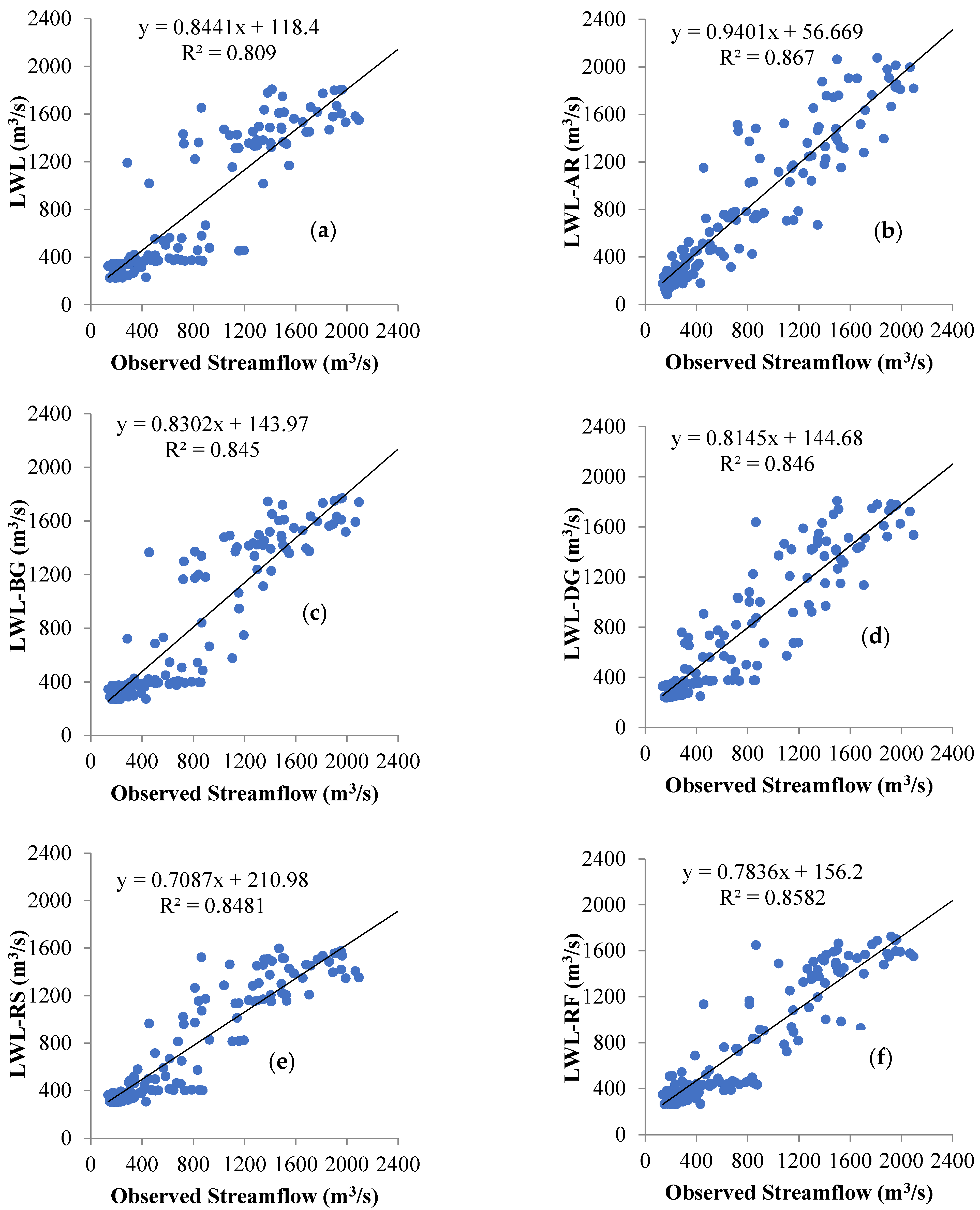
5. Results
6. Discussion
7. Conclusions
- The ensemble models are predominantly superior to the single LWL model for monthly streamflow forecasting.
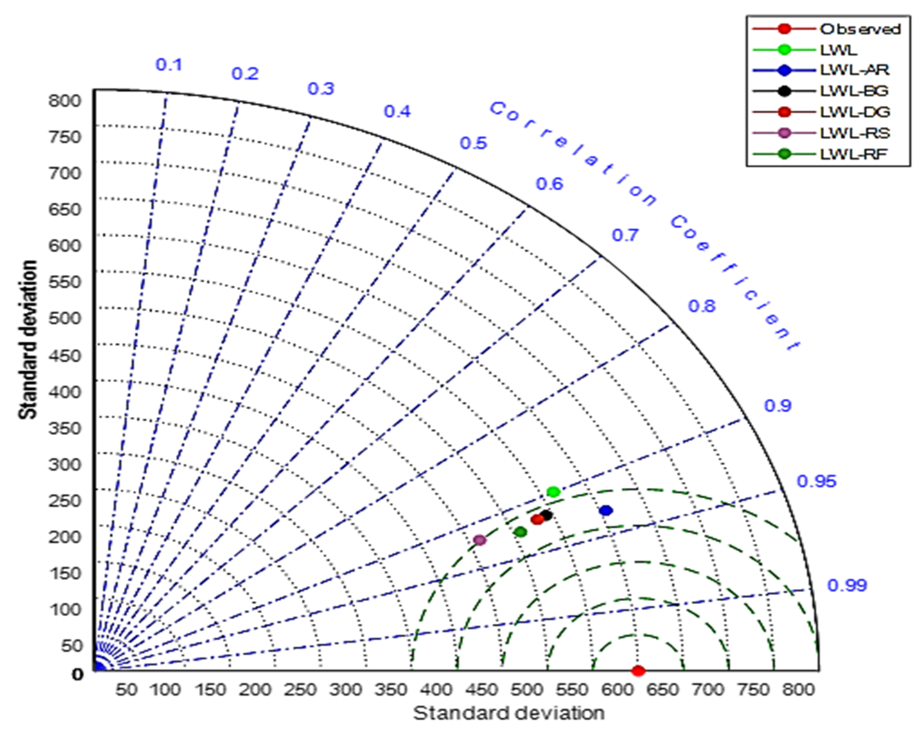
- Among the ensemble methods, the LWL-AR model surpasses the other models in both training and testing performances.
- The most accurate models are developed when the periodicity variable (MN, month number) is incorporated into the modeling process.
- Ensemble forecasting is a robust and promising alternative to the single forecasting of streamflow.
Author Contributions
Funding
Institutional Review Board Statement
Informed Consent Statement
Data Availability Statement
Conflicts of Interest
References
- Zhang, W.; Hu, Y.; Liu, J.; Wang, H.; Wei, J.; Sun, P.; Wu, L.; Zheng, H. Progress of ethylene action mechanism and its application on plant type formation in crops. Saudi J. Biol. Sci. 2020, 27, 1667–1673. [Google Scholar] [CrossRef] [PubMed]
- Adnan, R.M.; Liang, Z.; Heddam, S.; Zounemat-Kermani, M.; Kisi, O.; Li, B. Least square support vector machine and multivariate adaptive regression splines for streamflow prediction in mountainous basin using hydro-meteorological data as inputs. J. Hydrol. 2020, 586, 124371. [Google Scholar] [CrossRef]
- Yuan, X.; Chen, C.; Lei, X.; Yuan, Y.; Adnan, R.M. Monthly runoff forecasting based on LSTM–ALO model. Stoch. Environ. Res. Risk Assess. 2018, 32, 2199–2212. [Google Scholar] [CrossRef]
- Liu, J.; Liu, Y.; Wang, X. An environmental assessment model of construction and demolition waste based on system dynamics: A case study in Guangzhou. Environ. Sci. Pollut. Res. 2019, 27, 37237–37259. [Google Scholar] [CrossRef]
- Mehran, A.; AghaKouchak, A.; Nakhjiri, N.; Stewardson, M.J.; Peel, M.C.; Phillips, T.J.; Wada, Y.; Ravalico, J.K. Compounding Impacts of Human-Induced Water Stress and Climate Change on Water Availability. Sci. Rep. 2017, 7, 6282. [Google Scholar] [CrossRef] [Green Version]
- Zhang, C.; Zhang, B.; Li, W.; Liu, M. Response of streamflow to climate change and human activity in Xitiaoxi river basin in China. Hydrol. Process. 2014, 28, 43–50. [Google Scholar] [CrossRef]
- Adnan, R.M.; Liang, Z.; Parmar, K.S.; Soni, K.; Kisi, O. Modeling monthly streamflow in mountainous basin by MARS, GMDH-NN and DENFIS using hydroclimatic data. Neural Comput. Appl. 2021, 33, 2853–2871. [Google Scholar] [CrossRef]
- Gibbs, M.S.; Dandy, G.C.; Maier, H.R. Assessment of the ability to meet environmental water requirements in the Upper South East of South Australia. Stoch. Environ. Res. Risk Assess. 2013, 28, 39–56. [Google Scholar] [CrossRef]
- Kişi, Ö. Streamflow Forecasting Using Different Artificial Neural Network Algorithms. J. Hydrol. Eng. 2007, 12, 532–539. [Google Scholar] [CrossRef]
- Yossef, N.C.; Winsemius, H.; Weerts, A.; Van Beek, R.; Bierkens, M.F.P. Skill of a global seasonal streamflow forecasting system, relative roles of initial conditions and meteorological forcing. Water Resour. Res. 2013, 49, 4687–4699. [Google Scholar] [CrossRef] [Green Version]
- Aqil, M.; Kita, I.; Yano, A.; Nishiyama, S. A comparative study of artificial neural networks and neuro-fuzzy in continuous modeling of the daily and hourly behaviour of runoff. J. Hydrol. 2007, 337, 22–34. [Google Scholar] [CrossRef]
- Abudu, S.; Cui, C.-L.; King, J.P.; Abudukadeer, K. Comparison of performance of statistical models in forecasting monthly streamflow of Kizil River, China. Water Sci. Eng. 2010, 3, 269–281. [Google Scholar]
- Wang, W. Stochasticity, Nonlinearity and Forecasting of Streamflow Processes; IOS Press: Amsterdam, The Netherlands, 2006. [Google Scholar]
- Rajaee, T. Wavelet and Neuro-fuzzy Conjunction Approach for Suspended Sediment Prediction. CLEAN Soil Air Water 2010, 38, 275–286. [Google Scholar] [CrossRef]
- Mehdizadeh, S.; Fathian, F.; Safari, M.J.S.; Adamowski, J.F. Comparative assessment of time series and artificial intelligence models to estimate monthly streamflow: A local and external data analysis approach. J. Hydrol. 2019, 579, 124225. [Google Scholar] [CrossRef]
- Adnan, R.M.; Petroselli, A.; Heddam, S.; Santos, C.A.G.; Kisi, O. Short term rainfall-runoff modelling using several machine learning methods and a conceptual event-based model. Stoch. Environ. Res. Risk Assess. 2021, 35, 597–616. [Google Scholar] [CrossRef]
- Rahgoshay, M.; Feiznia, S.; Arian, M.; Hashemi, S.A.A. Simulation of daily suspended sediment load using an improved model of support vector machine and genetic algorithms and particle swarm. Arab. J. Geosci. 2019, 12. [Google Scholar] [CrossRef]
- Kim, C.M.; Parnichkun, M. Prediction of settled water turbidity and optimal coagulant dosage in drinking water treatment plant using a hybrid model of k-means clustering and adaptive neuro-fuzzy inference system. Appl. Water Sci. 2017, 7, 3885–3902. [Google Scholar] [CrossRef] [Green Version]
- Affes, Z.; Kaffel, R.H. Forecast Bankruptcy Using a Blend of Clustering and MARS Model—Case of US Banks. SSRN Electron. J. 2016, 281, 27–64. [Google Scholar] [CrossRef] [Green Version]
- Adnan, R.M.; Liang, Z.; Trajkovic, S.; Zounemat-Kermani, M.; Li, B.; Kisi, O. Daily streamflow prediction using optimally pruned extreme learning machine. J. Hydrol. 2019, 577, 123981. [Google Scholar] [CrossRef]
- Zhang, X.; Peng, Y.; Zhang, C.; Wang, B. Are hybrid models integrated with data preprocessing techniques suitable for monthly streamflow forecasting? Some experiment evidences. J. Hydrol. 2015, 530, 137–152. [Google Scholar] [CrossRef]
- Tongal, H.; Booij, M.J. Simulation and forecasting of streamflows using machine learning models coupled with base flow separation. J. Hydrol. 2018, 564, 266–282. [Google Scholar] [CrossRef]
- Ferreira, R.G.; da Silva, D.D.; Elesbon, A.A.A.; Fernandes-Filho, E.I.; Veloso, G.V.; Fraga, M.D.S.; Ferreira, L.B. Machine learning models for streamflow regionalization in a tropical watershed. J. Environ. Manag. 2021, 280, 111713. [Google Scholar] [CrossRef]
- Piazzi, G.; Thirel, G.; Perrin, C.; Delaigue, O. Sequential Data Assimilation for Streamflow Forecasting: Assessing the Sensitivity to Uncertainties and Updated Variables of a Conceptual Hydrological Model at Basin Scale. Water Resour. Res. 2021, 57, 57. [Google Scholar] [CrossRef]
- Saraiva, S.V.; Carvalho, F.D.O.; Santos, C.A.G.; Barreto, L.C.; Freire, P.K.D.M.M. Daily streamflow forecasting in Sobradinho Reservoir using machine learning models coupled with wavelet transform and bootstrapping. Appl. Soft Comput. 2021, 102, 107081. [Google Scholar] [CrossRef]
- Tyralis, H.; Papacharalampous, G.; Langousis, A. Super ensemble learning for daily streamflow forecasting: Large-scale demonstration and comparison with multiple machine learning algorithms. Neural Comput. Appl. 2021, 33, 3053–3068. [Google Scholar] [CrossRef]
- Zhang, K.; Ruben, G.B.; Li, X.; Li, Z.; Yu, Z.; Xia, J.; Dong, Z. A comprehensive assessment framework for quantifying climatic and anthropogenic contributions to streamflow changes: A case study in a typical semi-arid North China basin. Environ. Model. Softw. 2020, 128, 104704. [Google Scholar] [CrossRef]
- Yen, H.P.H.; Pham, B.T.; Van Phong, T.; Ha, D.H.; Costache, R.; Van Le, H.; Nguyen, H.D.; Amiri, M.; Van Tao, N.; Prakash, I. Locally weighted learning based hybrid intelligence models for groundwater potential mapping and modeling: A case study at Gia Lai province, Vietnam. Geosci. Front. 2021, 12, 101154. [Google Scholar] [CrossRef]
- Tuyen, T.T.; Jaafari, A.; Yen, H.P.H.; Nguyen-Thoi, T.; Van Phong, T.; Nguyen, H.D.; Van Le, H.; Phuong, T.T.M.; Nguyen, S.H.; Prakash, I.; et al. Mapping forest fire susceptibility using spatially explicit ensemble models based on the locally weighted learning algorithm. Ecol. Inform. 2021, 63, 101292. [Google Scholar] [CrossRef]
- Atkeson, C.G.; Moore, A.W.; Schaal, S. Locally Weighted Learning. Artif. Intell. Rev. 1997, 11, 11–73. [Google Scholar] [CrossRef]
- Ahmadianfar, I.; Jamei, M.; Chu, X. A novel Hybrid Wavelet-Locally Weighted Linear Regression (W-LWLR) Model for Electrical Conductivity (EC) Prediction in Surface Water. J. Contam. Hydrol. 2020, 232, 103641. [Google Scholar] [CrossRef] [PubMed]
- Kisi, O.; Ozkan, C. A New Approach for Modeling Sediment-Discharge Relationship: Local Weighted Linear Regression. Water Resour. Manag. 2016, 31, 1–23. [Google Scholar] [CrossRef]
- Chen, T.; Ren, J. Bagging for Gaussian process regression. Neurocomputing 2009, 72, 1605–1610. [Google Scholar] [CrossRef] [Green Version]
- Zhou, Y.; Tian, L.; Zhu, C.; Jin, X.; Sun, Y. Video Coding Optimization for Virtual Reality 360-Degree Source. IEEE J. Sel. Top. Signal Process. 2020, 14, 118–129. [Google Scholar] [CrossRef]
- Azhari, M.; Abarda, A.; Alaoui, A.; Ettaki, B.; Zerouaoui, J. Detection of Pulsar Candidates using Bagging Method. Procedia Comput. Sci. 2020, 170, 1096–1101. [Google Scholar] [CrossRef]
- Xue, X.; Zhang, K.; Tan, K.C.; Feng, L.; Wang, J.; Chen, G.; Zhao, X.; Zhang, L.; Yao, J. Affine Transformation-Enhanced Multifactorial Optimization for Heterogeneous Problems. IEEE Trans. Cybern. 2020, 1–15. [Google Scholar] [CrossRef] [PubMed]
- Stone, C.J. Additive Regression and Other Nonparametric Models. Ann. Stat. 1985, 13, 689–705. [Google Scholar] [CrossRef]
- Piegorsch, W.W.; Xiong, H.; Bhattacharya, R.N.; Lin, L. Benchmark Dose Analysis via Nonparametric Regression Modeling. Risk Anal. 2013, 34, 135–151. [Google Scholar] [CrossRef] [Green Version]
- Zhang, M.; Yang, Z.; Liu, L.; Zhou, D. Impact of renewable energy investment on carbon emissions in China—An empirical study using a nonparametric additive regression model. Sci. Total Environ. 2021, 785, 147109. [Google Scholar] [CrossRef]
- Ho, T.K. The random subspace method for constructing decision forests. IEEE Trans. Pattern Anal. Mach. Intell. 1998, 20, 832–844. [Google Scholar] [CrossRef] [Green Version]
- Havlíček, V.; Córcoles, A.D.; Temme, K.; Harrow, A.W.; Kandala, A.; Chow, J.M.; Gambetta, J.M. Supervised learning with quantum-enhanced feature spaces. Nat. Cell Biol. 2019, 567, 209–212. [Google Scholar] [CrossRef] [Green Version]
- Kuncheva, L.I.; Rodriguez, J.J.; Plumpton, C.O.; Linden, D.E.J.; Johnston, S.J. Random Subspace Ensembles for fMRI Classification. IEEE Trans. Med. Imaging 2010, 29, 531–542. [Google Scholar] [CrossRef]
- Pham, B.T.; Bui, D.T.; Prakash, I.; Dholakia, M. Hybrid integration of Multilayer Perceptron Neural Networks and machine learning ensembles for landslide susceptibility assessment at Himalayan area (India) using GIS. Catena 2017, 149, 52–63. [Google Scholar] [CrossRef]
- Ting, K.M.; Witten, I.H. Stacking Bagged and Dagged Models; University of Waikato: Hamilton, New Zealand, 1997. [Google Scholar]
- Yariyan, P.; Janizadeh, S.; Van Phong, T.; Nguyen, H.D.; Costache, R.; Van Le, H.; Pham, B.T.; Pradhan, B.; Tiefenbacher, J.P. Improvement of Best First Decision Trees Using Bagging and Dagging Ensembles for Flood Probability Mapping. Water Resour. Manag. 2020, 34, 3037–3053. [Google Scholar] [CrossRef]
- Zuo, C.; Chen, Q.; Tian, L.; Waller, L.; Asundi, A. Transport of intensity phase retrieval and computational imaging for partially coherent fields: The phase space perspective. Opt. Lasers Eng. 2015, 71, 20–32. [Google Scholar] [CrossRef]
- Tran, Q.C.; Minh, D.D.; Jaafari, A.; Al-Ansari, N.; Minh, D.D.; Van, D.T.; Nguyen, D.A.; Tran, T.H.; Ho, L.S.; Nguyen, D.H.; et al. Novel Ensemble Landslide Predictive Models Based on the Hyperpipes Algorithm: A Case Study in the Nam Dam Commune, Vietnam. Appl. Sci. 2020, 10, 3710. [Google Scholar] [CrossRef]
- Malek, A.G.; Mansoori, M.; Omranpour, H. Random forest and rotation forest ensemble methods for classification of epileptic EEG signals based on improved 1D-LBP feature extraction. Int. J. Imaging Syst. Technol. 2021, 31, 189–203. [Google Scholar] [CrossRef]
- Jiang, Q.; Shao, F.; Lin, W.; Gu, K.; Jiang, G.; Sun, H. Optimizing Multistage Discriminative Dictionaries for Blind Image Quality Assessment. IEEE Trans. Multimed. 2018, 20, 2035–2048. [Google Scholar] [CrossRef]
- Pham, B.T.; Jaafari, A.; Avand, M.; Al-Ansari, N.; Du, T.D.; Yen, H.P.H.; Van Phong, T.; Nguyen, D.H.; Van Le, H.; Mafi-Gholami, D.; et al. Performance Evaluation of Machine Learning Methods for Forest Fire Modeling and Prediction. Symmetry 2020, 12, 1022. [Google Scholar] [CrossRef]
- Zhang, K.; Zhang, J.; Ma, X.; Yao, C.; Zhang, L.; Yang, Y.; Wang, J.; Yao, J.; Zhao, H. History Matching of Naturally Fractured Reservoirs Using a Deep Sparse Autoencoder. SPE J. 2021, 1–22. [Google Scholar] [CrossRef]
- Zhao, C.; Li, J. Equilibrium Selection under the Bayes-Based Strategy Updating Rules. Symmetry 2020, 12, 739. [Google Scholar] [CrossRef]
- Adnan, R.M.; Zounemat-Kermani, M.; Kuriqi, A.; Kisi, O. Machine Learning Method in Prediction Streamflow Considering Periodicity Component. In Understanding Built Environment; Springer: Berlin/Heidelberg, Germany, 2020; pp. 383–403. [Google Scholar]
- Kisi, O.; Shiri, J.; Karimi, S.; Adnan, R.M. Three different adaptive neuro fuzzy computing techniques for forecasting long-period daily streamflows. In Big Data in Engineering Applications; Springer: Singapore, 2018; pp. 303–321. [Google Scholar]
- Alizamir, M.; Kisi, O.; Muhammad Adnan, R.; Kuriqi, A. Modelling reference evapotranspiration by combining neuro-fuzzy and evolutionary strategies. Acta Geophys. 2020, 68, 1113–1126. [Google Scholar] [CrossRef]
- Zhao, J.; Liu, J.; Jiang, J.; Gao, F. Efficient Deployment with Geometric Analysis for mmWave UAV Communications. IEEE Wirel. Commun. Lett. 2020, 9, 1. [Google Scholar] [CrossRef]
- Kişi, Ö. River flow forecasting and estimation using different artificial neural network techniques. Hydrol. Res. 2008, 39, 27–40. [Google Scholar] [CrossRef]
- Adnan, R.M.; Yuan, X.; Kisi, O.; Yuan, Y.; Tayyab, M.; Lei, X. Application of soft computing models in streamflow forecasting. In Proceedings of the Institution of Civil Engineers—Water Management; Thomas Telford Ltd.: London, UK, 2019; Volume 172, pp. 123–134. [Google Scholar] [CrossRef]
- Pham, B.T.; Jaafari, A.; Van Phong, T.; Yen, H.P.H.; Tuyen, T.T.; Van Luong, V.; Nguyen, H.D.; Van Le, H.; Foong, L.K. Improved flood susceptibility mapping using a best first decision tree integrated with ensemble learning techniques. Geosci. Front. 2021, 12, 101105. [Google Scholar] [CrossRef]


| Statistics | Whole Dataset (m3/s) 1965 to 2012 | M1 Dataset (m3/s) 2001 to 2012 | M2 Dataset (m3/s) 1989 to 2000 | M3 Dataset (m3/s) 1977 to 1988 | M4 Dataset (m3/s) 1965 to 1976 |
|---|---|---|---|---|---|
| Mean | 772.9 | 794.0 | 783.7 | 835.8 | 678.0 |
| Min. | 110.7 | 112.3 | 134.9 | 127.0 | 110.7 |
| Max. | 2824 | 2824 | 2426 | 2773 | 2014 |
| Skewness | 0.886 | 0.931 | 0.716 | 0.845 | 0.888 |
| Std. dev. | 609.2 | 645.1 | 600.6 | 651.7 | 514.1 |
| Variance | 371,069 | 416,106 | 360,780 | 424,712 | 264,330 |
| Parameter | Model | |||||
|---|---|---|---|---|---|---|
| LWL | AR | BG | DG | RS | RF | |
| Debug | False | False | False | False | False | False |
| Search algorithm | Linear NN search | - | - | - | - | - |
| Weighting kernel | 0 | - | - | - | - | - |
| Number of iterations | - | 14 | 12 | 10 | 10 | 11 |
| Shrinkage | - | 0.1 | - | - | - | - |
| Bag size percent | - | - | 100 | - | - | - |
| Seed | - | - | 1 | 1 | 1 | 1 |
| Number of folds | - | - | - | 10 | - | - |
| Verbose | - | - | - | False | - | - |
| Number of boosting iterations | - | 30 | - | - | - | - |
| Subspace size | - | - | - | - | 0.5 | - |
| Max group | - | - | - | - | - | 3 |
| Min group | - | - | - | - | - | 3 |
| Number of groups | - | - | - | - | - | False |
| Projection filter | - | - | - | - | - | PCA |
| Removed percentage | - | - | - | - | - | 50 |
| Metric | Data Set | Training | Testing | ||||||
|---|---|---|---|---|---|---|---|---|---|
| Input Combination | Input Combination | ||||||||
| I | II | III | IV | I | II | III | IV | ||
| RMSE | M1 | 358.6 | 300.3 | 295.5 | 255.9 | 365.8 | 308.6 | 311.4 | 295.4 |
| M2 | 358.7 | 303.7 | 275.5 | 242.1 | 397.0 | 370.2 | 369.5 | 328.0 | |
| M3 | 358.8 | 283.8 | 271.5 | 244.0 | 382.1 | 303 | 292.9 | 274.8 | |
| M4 | 362.3 | 306.5 | 300.4 | 252.3 | 397.9 | 342.2 | 312.4 | 277.7 | |
| Mean | 359.6 | 298.6 | 285.7 | 248.6 | 385.7 | 331.0 | 321.6 | 294.0 | |
| MAE | M1 | 282.6 | 227.7 | 226.0 | 183.5 | 271.0 | 231.3 | 241.4 | 207.7 |
| M2 | 279.9 | 227.0 | 210.1 | 178.8 | 306.9 | 263.9 | 265.0 | 222.2 | |
| M3 | 274.4 | 213.8 | 204.9 | 175.0 | 291.5 | 228.8 | 219.9 | 199.2 | |
| M4 | 281.5 | 230.8 | 229.0 | 183.5 | 309.8 | 257.2 | 240.9 | 200.0 | |
| Mean | 279.6 | 224.8 | 217.5 | 180.2 | 294.8 | 245.3 | 241.8 | 207.3 | |
| RAE | M1 | 52.24 | 42.09 | 41.78 | 35.92 | 57.57 | 49.12 | 51.27 | 44.12 |
| M2 | 55.67 | 44.14 | 41.39 | 35.57 | 56.68 | 48.74 | 48.95 | 41.03 | |
| M3 | 53.35 | 42.51 | 40.75 | 34.47 | 56.01 | 43.95 | 42.25 | 38.70 | |
| M4 | 55.47 | 45.47 | 44.53 | 33.67 | 57.56 | 47.79 | 44.75 | 38.16 | |
| Mean | 54.18 | 43.55 | 42.11 | 34.91 | 56.96 | 47.40 | 46.81 | 40.50 | |
| RRSE | M1 | 58.80 | 47.42 | 46.64 | 39.94 | 65.81 | 57.8 | 58.32 | 55.32 |
| M2 | 60.51 | 49.62 | 46.19 | 40.85 | 63.60 | 56.34 | 56.24 | 49.91 | |
| M3 | 58.63 | 47.88 | 45.80 | 40.90 | 60.42 | 50.43 | 48.74 | 44.08 | |
| M4 | 60.74 | 51.38 | 49.09 | 41.72 | 61.62 | 52.99 | 48.38 | 46.24 | |
| Mean | 59.67 | 49.08 | 46.93 | 40.85 | 62.86 | 54.39 | 52.92 | 48.89 | |
| R | M1 | 0.659 | 0.776 | 0.783 | 0.841 | 0.594 | 0.672 | 0.676 | 0.746 |
| M2 | 0.642 | 0.750 | 0.792 | 0.834 | 0.612 | 0.687 | 0.694 | 0.759 | |
| M3 | 0.658 | 0.773 | 0.792 | 0.834 | 0.629 | 0.746 | 0.762 | 0.809 | |
| M4 | 0.634 | 0.736 | 0.759 | 0.826 | 0.619 | 0.723 | 0.757 | 0.789 | |
| Mean | 0.648 | 0.759 | 0.782 | 0.834 | 0.614 | 0.707 | 0.722 | 0.776 | |
| Metric | Dataset | Training | Testing | ||||||
|---|---|---|---|---|---|---|---|---|---|
| Input Combination | Input Combination | ||||||||
| I | II | III | IV | I | II | III | IV | ||
| RMSE | M1 | 321.0 | 184.5 | 162.4 | 143.7 | 327.5 | 292.8 | 293.3 | 261.9 |
| M2 | 310.0 | 183.8 | 170.3 | 128.3 | 407.8 | 334.4 | 315.2 | 273.5 | |
| M3 | 306.9 | 174.0 | 152.1 | 138.4 | 373.6 | 264.4 | 258.8 | 223.9 | |
| M4 | 314.2 | 193.3 | 169.1 | 139.1 | 377.6 | 294.6 | 284.2 | 242.9 | |
| Mean | 313.0 | 183.9 | 163.5 | 137.4 | 371.6 | 296.6 | 287.9 | 250.6 | |
| MAE | M1 | 248.1 | 135.8 | 115.8 | 97.47 | 247.2 | 199.8 | 195.9 | 171.1 |
| M2 | 241.6 | 130.2 | 120 | 88.47 | 310.9 | 224.2 | 209.4 | 168.6 | |
| M3 | 232.2 | 125.1 | 104.8 | 95.72 | 292.1 | 191.7 | 183.8 | 150.7 | |
| M4 | 242.6 | 136.6 | 117.8 | 95.72 | 295.1 | 200.4 | 198.6 | 156.0 | |
| Mean | 241.1 | 131.9 | 114.6 | 94.30 | 286.3 | 204.0 | 196.9 | 161.6 | |
| RAE | M1 | 45.87 | 25.11 | 21.43 | 17.70 | 52.51 | 42.44 | 41.61 | 33.90 |
| M2 | 48.04 | 25.31 | 23.32 | 17.60 | 57.43 | 41.41 | 38.67 | 31.13 | |
| M3 | 45.15 | 24.87 | 20.83 | 18.95 | 56.11 | 36.82 | 35.31 | 28.95 | |
| M4 | 47.79 | 26.92 | 23.20 | 18.60 | 54.83 | 37.23 | 36.89 | 31.80 | |
| Mean | 46.71 | 25.55 | 22.20 | 18.21 | 55.22 | 39.48 | 38.12 | 31.45 | |
| RRSE | M1 | 50.69 | 29.13 | 25.64 | 21.86 | 61.33 | 54.83 | 54.93 | 45.49 |
| M2 | 52.29 | 30.03 | 27.83 | 21.64 | 62.06 | 50.90 | 47.96 | 41.62 | |
| M3 | 50.15 | 29.36 | 25.65 | 23.48 | 62.18 | 44.00 | 43.08 | 23.26 | |
| M4 | 52.67 | 32.4 | 28.34 | 23.31 | 58.47 | 45.63 | 44.02 | 40.57 | |
| Mean | 51.45 | 30.23 | 26.87 | 22.57 | 61.01 | 48.84 | 47.50 | 37.74 | |
| R | M1 | 0.743 | 0.916 | 0.935 | 0.953 | 0.621 | 0.740 | 0.733 | 0.823 |
| M2 | 0.728 | 0.910 | 0.924 | 0.953 | 0.612 | 0.743 | 0.773 | 0.828 | |
| M3 | 0.750 | 0.914 | 0.935 | 0.945 | 0.616 | 0.808 | 0.821 | 0.867 | |
| M4 | 0.723 | 0.903 | 0.922 | 0.947 | 0.658 | 0.794 | 0.806 | 0.835 | |
| Mean | 0.736 | 0.911 | 0.929 | 0.950 | 0.627 | 0.771 | 0.783 | 0.838 | |
| Metric | Dataset | Training | Testing | ||||||
|---|---|---|---|---|---|---|---|---|---|
| Input Combination | Input Combination | ||||||||
| I | II | III | IV | I | II | III | IV | ||
| RMSE | M1 | 363.6 | 290.0 | 272.9 | 240.9 | 345.5 | 294.0 | 274.3 | 261.2 |
| M2 | 352.3 | 285.8 | 266.5 | 237.9 | 398.1 | 340.6 | 345.2 | 306.5 | |
| M3 | 336.6 | 262.0 | 250.7 | 229.4 | 359.4 | 292.8 | 276.1 | 255.3 | |
| M4 | 342.8 | 289.5 | 272.6 | 250.5 | 376.4 | 319.1 | 294.7 | 258.8 | |
| Mean | 348.8 | 281.8 | 265.7 | 239.7 | 369.9 | 311.6 | 297.6 | 270.5 | |
| MAE | M1 | 284.4 | 224.2 | 212.6 | 177.4 | 269.0 | 226.6 | 218.5 | 187.7 |
| M2 | 273.6 | 217.4 | 202.1 | 174.8 | 310.9 | 243.5 | 247.3 | 208.0 | |
| M3 | 265.9 | 202.0 | 191.0 | 169.8 | 279.4 | 223.6 | 209.5 | 191.7 | |
| M4 | 270.6 | 220.8 | 205.1 | 183.0 | 300.5 | 248.6 | 225.3 | 182.8 | |
| Mean | 273.6 | 216.1 | 202.7 | 176.3 | 290.0 | 235.6 | 225.2 | 192.6 | |
| RAE | M1 | 52.58 | 41.45 | 39.31 | 32.90 | 57.13 | 48.14 | 46.40 | 38.83 |
| M2 | 53.19 | 42.27 | 39.83 | 34.45 | 57.42 | 44.97 | 45.69 | 38.43 | |
| M3 | 52.88 | 40.16 | 37.98 | 33.77 | 53.68 | 42.95 | 40.24 | 34.88 | |
| M4 | 53.32 | 43.50 | 39.88 | 35.57 | 55.83 | 46.19 | 41.86 | 36.83 | |
| Mean | 52.99 | 41.85 | 39.25 | 34.17 | 56.02 | 45.56 | 43.55 | 37.24 | |
| RRSE | M1 | 57.42 | 45.79 | 43.10 | 38.04 | 64.71 | 55.05 | 51.37 | 48.46 |
| M2 | 57.56 | 46.71 | 44.67 | 39.88 | 60.58 | 51.83 | 52.54 | 46.65 | |
| M3 | 56.77 | 44.19 | 42.29 | 38.70 | 59.82 | 48.73 | 45.96 | 40.45 | |
| M4 | 57.47 | 48.53 | 44.54 | 40.94 | 58.30 | 49.42 | 45.64 | 42.48 | |
| Mean | 57.31 | 46.31 | 43.65 | 39.39 | 60.85 | 51.26 | 48.88 | 44.51 | |
| R | M1 | 0.672 | 0.794 | 0.817 | 0.859 | 0.590 | 0.694 | 0.743 | 0.781 |
| M2 | 0.669 | 0.783 | 0.803 | 0.845 | 0.627 | 0.736 | 0.731 | 0.796 | |
| M3 | 0.679 | 0.808 | 0.824 | 0.854 | 0.646 | 0.762 | 0.789 | 0.845 | |
| M4 | 0.671 | 0.766 | 0.803 | 0.834 | 0.661 | 0.760 | 0.799 | 0.821 | |
| Mean | 0.673 | 0.788 | 0.812 | 0.848 | 0.631 | 0.738 | 0.766 | 0.811 | |
| Metric | Dataset | Training | Testing | ||||||
|---|---|---|---|---|---|---|---|---|---|
| Input Combination | Input Combination | ||||||||
| I | II | III | IV | I | II | III | IV | ||
| RMSE | M1 | 369.2 | 310.1 | 279.1 | 241.0 | 320.3 | 274.1 | 259.0 | 249.4 |
| M2 | 355.4 | 296.3 | 270.9 | 264.8 | 390.6 | 335.8 | 326.4 | 298.8 | |
| M3 | 338.3 | 285.6 | 262.6 | 234.5 | 349.6 | 288.2 | 253.9 | 233.5 | |
| M4 | 346.6 | 299.3 | 271.7 | 239.5 | 337.6 | 324.9 | 286.0 | 247.1 | |
| Mean | 352.4 | 297.8 | 271.1 | 245.0 | 349.5 | 305.8 | 281.3 | 257.2 | |
| MAE | M1 | 286.0 | 236.6 | 211.7 | 171.3 | 248.0 | 217.4 | 206.0 | 191.1 |
| M2 | 275.2 | 225.8 | 201.7 | 194.0 | 299.3 | 246.8 | 229.3 | 209.4 | |
| M3 | 262.2 | 220.1 | 200.1 | 166.9 | 274.3 | 227.2 | 197.8 | 181.3 | |
| M4 | 267.5 | 225.2 | 207.3 | 181.4 | 298.8 | 252.2 | 220.8 | 179.4 | |
| Mean | 272.7 | 226.9 | 205.2 | 178.4 | 280.1 | 235.9 | 213.5 | 190.3 | |
| RAE | M1 | 52.87 | 43.75 | 39.14 | 31.67 | 52.67 | 46.18 | 43.76 | 39.85 |
| M2 | 53.51 | 43.89 | 39.21 | 37.71 | 55.28 | 45.59 | 42.36 | 38.68 | |
| M3 | 52.15 | 43.77 | 39.80 | 32.89 | 52.69 | 43.66 | 37.99 | 33.34 | |
| M4 | 52.70 | 44.37 | 40.84 | 36.07 | 55.52 | 46.85 | 41.02 | 36.72 | |
| Mean | 52.81 | 43.95 | 39.75 | 34.59 | 54.04 | 45.57 | 41.28 | 37.15 | |
| RRSE | M1 | 58.30 | 48.97 | 44.07 | 38.06 | 59.98 | 51.32 | 48.50 | 44.56 |
| M2 | 58.07 | 48.42 | 44.27 | 43.28 | 59.44 | 51.10 | 49.67 | 45.48 | |
| M3 | 57.06 | 48.18 | 44.30 | 39.30 | 58.18 | 47.96 | 42.26 | 38.26 | |
| M4 | 58.09 | 50.18 | 45.54 | 40.40 | 58.64 | 50.32 | 44.29 | 41.52 | |
| Mean | 57.88 | 48.94 | 44.55 | 40.26 | 59.06 | 50.18 | 46.18 | 42.46 | |
| R | M1 | 0.663 | 0.766 | 0.814 | 0.867 | 0.623 | 0.724 | 0.753 | 0.803 |
| M2 | 0.663 | 0.771 | 0.806 | 0.815 | 0.643 | 0.753 | 0.778 | 0.797 | |
| M3 | 0.676 | 0.774 | 0.815 | 0.848 | 0.663 | 0.774 | 0.824 | 0.847 | |
| M4 | 0.663 | 0.753 | 0.797 | 0.841 | 0.659 | 0.764 | 0.821 | 0.828 | |
| Mean | 0.666 | 0.766 | 0.808 | 0.843 | 0.647 | 0.754 | 0.794 | 0.819 | |
| Metric | Dataset | Training | Testing | ||||||
|---|---|---|---|---|---|---|---|---|---|
| Input Combination | Input Combination | ||||||||
| I | II | III | IV | I | II | III | IV | ||
| RMSE | M1 | 371.3 | 329.9 | 287.0 | 270.4 | 351.4 | 302.1 | 274.1 | 248.7 |
| M2 | 358.7 | 319.8 | 301.1 | 282.0 | 397.0 | 362.1 | 371.6 | 345.5 | |
| M3 | 359.8 | 317.2 | 279.3 | 268.2 | 382.1 | 326.8 | 302.7 | 242.8 | |
| M4 | 362.3 | 296.7 | 319.8 | 280.4 | 397.9 | 344.3 | 319.2 | 302.5 | |
| Mean | 363.0 | 315.9 | 296.8 | 275.3 | 382.1 | 333.8 | 316.9 | 284.9 | |
| MAE | M1 | 282.6 | 261.1 | 225.2 | 200.3 | 271.0 | 248.1 | 221.8 | 192.7 |
| M2 | 279.9 | 238.0 | 231.8 | 207.2 | 306.9 | 295.5 | 274.1 | 243.0 | |
| M3 | 274.4 | 245.1 | 215.7 | 205.9 | 291.5 | 263.8 | 238.5 | 191.4 | |
| M4 | 281.5 | 248.6 | 238.0 | 219.3 | 309.8 | 276.7 | 240.7 | 228.3 | |
| Mean | 279.6 | 248.2 | 227.7 | 208.2 | 294.8 | 271.0 | 243.8 | 213.9 | |
| RAE | M1 | 52.25 | 46.76 | 41.64 | 37.09 | 57.56 | 52.68 | 47.11 | 40.66 |
| M2 | 55.68 | 49.13 | 45.06 | 40.29 | 56.68 | 53.43 | 50.63 | 44.88 | |
| M3 | 53.35 | 50.64 | 42.51 | 40.57 | 56.01 | 51.27 | 45.81 | 37.03 | |
| M4 | 55.47 | 48.78 | 49.13 | 43.62 | 57.56 | 54.41 | 44.73 | 42.41 | |
| Mean | 54.19 | 48.83 | 44.59 | 40.39 | 56.95 | 52.95 | 47.07 | 41.25 | |
| RRSE | M1 | 58.63 | 49.88 | 45.32 | 42.70 | 65.81 | 61.71 | 51.32 | 45.47 |
| M2 | 60.51 | 55.97 | 49.20 | 46.08 | 60.42 | 58.54 | 56.56 | 52.58 | |
| M3 | 58.80 | 54.89 | 46.82 | 44.96 | 63.60 | 57.68 | 50.39 | 41.39 | |
| M4 | 60.74 | 54.83 | 55.97 | 47.30 | 61.62 | 57.72 | 49.43 | 46.86 | |
| Mean | 59.67 | 53.89 | 49.33 | 45.26 | 62.86 | 58.91 | 51.93 | 46.58 | |
| R | M1 | 0.659 | 0.676 | 0.806 | 0.837 | 0.594 | 0.637 | 0.736 | 0.796 |
| M2 | 0.642 | 0.714 | 0.769 | 0.814 | 0.629 | 0.659 | 0.702 | 0.773 | |
| M3 | 0.659 | 0.682 | 0.790 | 0.821 | 0.612 | 0.676 | 0.750 | 0.848 | |
| M4 | 0.634 | 0.679 | 0.714 | 0.792 | 0.619 | 0.671 | 0.769 | 0.815 | |
| Mean | 0.649 | 0.688 | 0.770 | 0.816 | 0.614 | 0.661 | 0.739 | 0.808 | |
| Metric | Dataset | Training | Testing | ||||||
|---|---|---|---|---|---|---|---|---|---|
| Input Combination | Input Combination | ||||||||
| I | II | III | IV | I | II | III | IV | ||
| RMSE | M1 | 371.3 | 259.9 | 261.7 | 225.4 | 351.4 | 289.8 | 278.3 | 232.4 |
| M2 | 359.8 | 271.7 | 269.4 | 229.1 | 397.0 | 307.4 | 336.3 | 300.2 | |
| M3 | 358.7 | 242.9 | 253.0 | 213.8 | 382.1 | 265.6 | 266.3 | 229.4 | |
| M4 | 362.3 | 271.0 | 311.5 | 230.6 | 397.9 | 297.3 | 311.4 | 266.4 | |
| Mean | 363.0 | 261.4 | 273.9 | 224.7 | 382.1 | 290.0 | 298.1 | 257.1 | |
| MAE | M1 | 282.6 | 196.2 | 200.0 | 167.4 | 271.0 | 218.0 | 212.8 | 195.7 |
| M2 | 274.4 | 203.4 | 205.2 | 165.0 | 306.9 | 223.1 | 237.4 | 201.7 | |
| M3 | 279.9 | 184.2 | 193.0 | 160.0 | 291.5 | 195.5 | 195.6 | 173.0 | |
| M4 | 281.5 | 204.1 | 237.8 | 167.3 | 309.8 | 227.8 | 237.8 | 175.7 | |
| Mean | 279.6 | 197.0 | 209.0 | 164.9 | 294.8 | 216.1 | 220.9 | 186.5 | |
| RAE | M1 | 52.25 | 36.27 | 36.97 | 30.96 | 57.57 | 46.30 | 45.19 | 37.31 |
| M2 | 53.35 | 39.55 | 39.90 | 32.07 | 56.68 | 41.20 | 43.86 | 37.25 | |
| M3 | 55.68 | 36.62 | 38.38 | 31.36 | 56.01 | 37.56 | 37.57 | 33.23 | |
| M4 | 55.47 | 40.22 | 44.18 | 32.96 | 57.56 | 42.32 | 44.18 | 36.37 | |
| Mean | 54.19 | 38.17 | 39.86 | 31.84 | 56.96 | 41.85 | 42.70 | 36.04 | |
| RRSE | M1 | 58.63 | 41.03 | 41.33 | 35.59 | 65.81 | 54.27 | 52.11 | 42.96 |
| M2 | 58.80 | 44.41 | 44.03 | 37.44 | 60.42 | 46.78 | 51.17 | 45.68 | |
| M3 | 60.51 | 40.98 | 42.68 | 36.06 | 63.60 | 44.21 | 44.32 | 38.68 | |
| M4 | 60.74 | 45.42 | 48.24 | 38.66 | 61.62 | 46.04 | 48.24 | 41.26 | |
| Mean | 59.67 | 42.96 | 44.07 | 36.94 | 62.86 | 47.83 | 48.96 | 42.15 | |
| R | M1 | 0.659 | 0.834 | 0.830 | 0.88 | 0.594 | 0.714 | 0.753 | 0.821 |
| M2 | 0.659 | 0.805 | 0.806 | 0.869 | 0.629 | 0.787 | 0.750 | 0.806 | |
| M3 | 0.642 | 0.835 | 0.819 | 0.882 | 0.612 | 0.808 | 0.805 | 0.858 | |
| M4 | 0.634 | 0.796 | 0.771 | 0.856 | 0.619 | 0.799 | 0.771 | 0.846 | |
| Mean | 0.649 | 0.818 | 0.807 | 0.872 | 0.614 | 0.777 | 0.770 | 0.833 | |
Publisher’s Note: MDPI stays neutral with regard to jurisdictional claims in published maps and institutional affiliations. |
© 2021 by the authors. Licensee MDPI, Basel, Switzerland. This article is an open access article distributed under the terms and conditions of the Creative Commons Attribution (CC BY) license (https://creativecommons.org/licenses/by/4.0/).
Share and Cite
Adnan, R.M.; Jaafari, A.; Mohanavelu, A.; Kisi, O.; Elbeltagi, A. Novel Ensemble Forecasting of Streamflow Using Locally Weighted Learning Algorithm. Sustainability 2021, 13, 5877. https://doi.org/10.3390/su13115877
Adnan RM, Jaafari A, Mohanavelu A, Kisi O, Elbeltagi A. Novel Ensemble Forecasting of Streamflow Using Locally Weighted Learning Algorithm. Sustainability. 2021; 13(11):5877. https://doi.org/10.3390/su13115877
Chicago/Turabian StyleAdnan, Rana Muhammad, Abolfazl Jaafari, Aadhityaa Mohanavelu, Ozgur Kisi, and Ahmed Elbeltagi. 2021. "Novel Ensemble Forecasting of Streamflow Using Locally Weighted Learning Algorithm" Sustainability 13, no. 11: 5877. https://doi.org/10.3390/su13115877