Estimation of Fuzzy Parameters in the Linear Muskingum Model with the Aid of Particle Swarm Optimization

Abstract

The Muskingum method is one of the widely used methods for lumped flood routing in natural rivers. Calibration of its parameters remains an active challenge for the researchers. The task has been mostly addressed by using crisp numbers, but fuzzy seems a reasonable alternative to account for parameter uncertainty. In this work, a fuzzy Muskingum model is proposed where the assessment of the outflow as a fuzzy quantity is based on the crisp linear Muskingum method but with fuzzy parameters as inputs. This calculation can be achieved based on the extension principle of the fuzzy sets and logic. The critical point is the calibration of the proposed fuzzy extension of the Muskingum method. Due to complexity of the model, the particle swarm optimization (PSO) method is used to enable the use of a simulation process for each possible solution that composes the swarm. A weighted sum of several performance criteria is used as the fitness function of the PSO. The function accounts for the inclusive constraints (the property that the data must be included within the produced fuzzy band) and for the magnitude of the fuzzy band, since large uncertainty may render the model non-functional. Four case studies from the references are used to benchmark the proposed method, including smooth, double, and non-smooth data and a complex, real case study that shows the advantages of the approach. The use of fuzzy parameters is closer to the uncertain nature of the problem. The new methodology increases the reliability of the prediction. Furthermore, the produced fuzzy band can include, to a significant degree, the observed data and the output of the existent crisp methodologies even if they include more complex assumptions.

1. Introduction

Flood risk management is a key component in sustainable water resources management. Floods impact both individuals and communities, producing harmful consequences of social, economic, and environmental implications. Negative impacts of flooding include loss of human life, destruction of crops, damage to essential infrastructure, and disruption of the value chain. Many flood risk management strategies are based on operational early waring schemes that predict the arrival of the flood wave and enable civil protection actions to safeguard life and property. The prediction of the outflow hydrograph for a river’s reach given a specific inflow hydrograph is, therefore, an important issue in water resources management. Hydrological forecasting requires a sound understanding of the physical mechanisms that control the propagation of flood waves along rivers. Mathematical models for flood routing are based on the unsteady flow Saint-Venant equations. Numerical solutions of the flow equations are complex, and thus, simplified versions are preferred in operational flood forecasting schemes. Various methods have been developed for this purpose, which may be categorized into three distinct groups [1,2]: (1) the distributed (or hydraulic) methods (e.g., dynamic wave, diffusion wave, and kinematic wave models), which are based on the mass conservation and momentum transport equations; (2) the lumped (or hydrologic) methods (in which the linear and nonlinear Muskingum models [3] are widely used); and (3) the semi-distributed or hybrid methods (e.g., Muskingum–Cunge family models [456]). This work is focused on enhancing models of the third category using fuzzy sets and logic.

Lumped models estimate the flood hydrograph at a downstream section of the river from the flood hydrograph at the upstream section without considering explicitly the river characteristics between the upstream and the downstream sections. These models use the one-dimensional continuity equation along with a storage equation in the calibration and verification steps.

The Muskingum method for natural streamflow routing, first proposed by McCarthy (1938) [3] in the Muskingum River basin in Ohio, is a widely applied hydrologic method [7]. It is a lumped method which cannot provide the outflow at the intermediate sections. However, these models are very popular since, in most cases, the scarcity of field data prevents the use of the Saint-Venant equations to route floods in rivers, as occurs in the second category of river-reach routing [8].

The widely-used linear Muskingum method depends on two parameters: K and x [9]. Originally, the graphical method was developed to determine the parameters of the widely-used Muskingum linear equation. As is widely known, the graphical solution is based on the graphical representation of the storage versus the weighted discharge as a function of x. The preferred value of x is the one that produces the narrowest loop (e.g., Wilson, 1974 [10]). Next, some techniques based either on linear programming or on linear regression were developed [11]. However, the use of the regression-based techniques can lead to unreasonable values for K, x (e.g., [12]), due to an overtraining behavior.

The use of the nonlinear storage equation within the Muskingum method increases the number of model parameters, but it is closer to reality. However, the nonlinear storage equation increases the difficulty of the calibration process. Various mathematical-hydrological methodologies are developed to calibrate the river-routing models by using a nonlinear approach regarding the relation of the reach storage. For instance, according to the segmented least-squares method (S-LSM) (Gill 1978) [13], the whole available data are subdivided into several groups based on the storage values. It is then assumed that K and x remain constant in each subgroup, and hence, for each subgroup, the least square analysis is used. Therefore, the optimization procedure is based on the minimization between the estimated storage and the existent storage.

Next, a directly (global) nonlinear formulation of the Muskingum method (regarding the reach storage) was proposed by several authors with the use of a nonlinear form for the storage. For instance, [14] used several mathematical techniques to minimize the sum of the squares of deviations between observed channel storage and computed channel storage.

Similarly, the nonlinear least squares method (NL-LSM) [15], the Lagrange multiplier method (LMM) [7], and the Broyden–Fletcher–Goldfarb–Shanno (BFGS) technique [16] have been exploited for assessing the parameter values of the models. Das (2004) [7] and Geem (2006) [15] proposed an optimization model whose objective function emphasizes the determination of a set of parameter values that minimizes the error between model-predicted and observed outflows. Das (2004) [7] considered the validation of the storage-discharge relation by using the Lagrange multipliers.

However, these techniques have the drawbacks of a complex derivative requirement and/or good initial vector consideration [17,18]. For example, the BFGS technique (Geem 2006) [16], although it reached the best solution ever found, relies heavily on the consideration of the initial vector [17]. Hence, several researchers have proposed various phenomenon-mimicking algorithms where an initial population of possible solutions is used instead of an initial vector. For instance, the genetic algorithm (GA) [19] (Mohan 1997), harmony search (HS) (Kim et al., 2001) [20], particle swarm optimization (PSO) (Chu and Chang 2009) [21], differential evolution (DE) (Xu et al., 2011) [22], parameter-setting free harmony search (PSFHS) algorithm [23], and modified honey bee mating optimization (MHBMO) algorithm (Niazkar and Afzali 2015) [24] were developed to achieve the calibration of the nonlinear Muskingum method (Niazkar and Afzali 2016) [25].

In order to improve the optimum solution, several authors proposed hybrid optimization algorithms that combine the heuristic and the derivatives-based algorithms from a mathematical point of view. Two steps are mainly considered. In the first step, one of search-based, phenomenon-mimicking algorithms, which requires no initial guess, is exploited to assess the Muskingum parameters. Afterwards, the obtained values for nonlinear Muskingum parameters are utilized as the first initial vector for the second step in which a deterministic, derivatives-based method continues the routing simulation optimization (Niazkar and Afzali 2016) [25]. For instance, in Karahan et al., 2015 [18], the HS algorithm (global search) searched the optimum solution with multiple solution vectors, and then the BFGS algorithm (local search) adjusted the results of the HS algorithm by getting its results as the new initial solution [18]. A critical point is that most of the suitability measures are based on the comparison between the observed and the predicted outflow, whilst the other older works, such as [13,14], are focused on the storage equation (as can be seen from the objective function used).

In addition, several authors proposed other innovations in the nonlinear Muskingum relation. Karahan et al., 2015 [18] proposed the use of the cuckoo search algorithm (which also uses an initial population) during the calibration of the model parameters by also including the lateral flow. Easa (2015) [26] proposed to increase performance using continuous and discontinuous parameters expressed as a function of a dimensionless inflow variable. In addition, Farzin et al., 2018 [27] proposed the multi-reach Muskingum method to enhance the accuracy of the Muskingum method. The river under study was divided into several smaller reaches, and hence, for each reach, routing was applied separately. However, if there are no data in intermediate sections, it is not obvious that the intermediate outcomes can be used to estimate the outflow at these sections, and therefore, the method could be characterized as a black box model rather than a conceptual model.

Regarding the application of the fuzzy sets and logic methods in these types of problems, most of the proposed models are based on the adaptive network-based fuzzy inference systems (ANFIS) implementation. ANFIS is a neuro-adaptive learning technique which provides a hybrid method for the fuzzy modeling procedure to learn information based on a data set. Therefore, it can be seen as a neuro-fuzzy approach. It is very popular because of the corresponding toolbox made available in MATLAB. In many hydraulic applications, the ANFIS method is widely used, providing very good results; however, it seems that sometimes it was solely utilized as a black-box model without any specific utilization of the produced fuzzy rules. Chu, 2009 [28] proposed the combined application of fuzzy inference system (FIS) and Muskingum model in flood routing. The implementation is based on the ANFIS toolbox of MATLAB. Three points of this methodology must be noted. The first one is that the Muskingum method is used indirectly in the structure of the model (neither the evaluation of K or x takes place). The second point is that the output (outflow) for each time step is a crisp number and not a fuzzy number. Thirdly, based on the ANFIS method, a large amount of data is required.

Another idea is to use the fuzzy linear regression to calibrate the linear Muskingum method instead of the crisp linear regression as O’Donnel (1985) [11] proposed. Spiliotis and Garrote (2017) [29] proposed the calibration of the Muskingum parameters based on fuzzy linear regression. Therefore, instead of the crisp coefficient of the O’Donnel (1985) method [11], the coefficients are proposed to be fuzzy symmetric triangular numbers. This implies that, in contrast with the widely used ANFIS, the output (outflow) of the proposed model is a fuzzy number. Furthermore, based on the Tanaka (1987) [30] fuzzy regression implementation, all the observed data (regarding the outflow) are forced to be included in the produced fuzzy band aiming at its minimum width. Instead of the identification of the parameters K, x, the problem is oriented to the determination of the corresponding regression coefficient. Another point of view is that, based on the problem itself, the constant term of the usual regression model must be removed [29]. The relevant feature of articles mentioned in this paragraph is that they contain methodologies that produce a fuzzy outflow as a final output for the channel-routing problem.

However, the fuzzy linear regression of Tanaka (1987) [30] is heavily influenced by the existence of outliers, which can extremely enlarge the spread of the model. Hence, Spiliotis and Garrote, 2017 [29] proposed the use of a fuzzy linear regression model that is modified by incorporating ideas from the field of goal programming. Spiliotis et al., 2018 [12] expanded the methodology by including the lateral flow on the basis of the O’Donnel article [11]. As it was noted by the authors, an interesting point is that sometimes the produced fuzzy coefficients cannot correspond to the physical meaning of the storage equation, and hence, the model leads to a rather metric or black-box method.

In this work, a hybrid, fuzzy-based methodology is proposed. The proposed method consists of two main ideas. Firstly, the linear Muskingum model is adopted. The parameters K, x and α (where lateral flow occurs) are selected to be fuzzy symmetrical triangular numbers to avoid any irrational training as may occur in the case of the fuzzy linear regression. Hence, the methods produce a fuzzy estimation of the outflow based on the (crisp) Muskingum function to predict the outflow. Mathematically, the application of a crisp function using fuzzy parameters can be treated based on the extension principle of the fuzzy sets and logic. Secondly, the calibration is addressed by using a hybrid optimization procedure. In this article, the particle swarm optimization method (PSO) is used. Hence, there is no need to predict an initial solution. For each possible solution based on the (considered) values of the fuzzy parameters K, x and α, the outflow is calculated. The outflow will be a fuzzy number, whilst its determination is based on the extension principle. Unfortunately, the implementation of the extension principle leads to some sub-optimization problems but without difficult constraints. The solvability of these sub-optimization problems is discussed in the methodology section.

Each possible solution is evaluated based on the degree of inclusion of the real data within the produced fuzzy band. This criterion should be included in the formulation of the fitness function of the heuristic optimization method. However, other criteria will be added which will be discussed in the methodology section. For instance, a fuzzy solution with a very large band will contain all the data, but this information is non-functional. Therefore, the fitness function must contain not only the inclusion degree but the magnitude of the fuzzy band, etc. In PSO, the values of the fitness function of the swarm and the use of random numbers determine the movement of the swarm, that is, the positions of the new possible solutions. The procedure is finished by considering a maximum number of iterations.

Three classical case studies from the references are widely used to benchmark the variations of the Muskingum method. These three case studies include: (1) smooth outflow (Wilson 1974 [10]), (2) double-peak outflow (Viessman and Lewis 2003) [9], and (3) non-smooth outflow with lateral flow (O’Donnel 1985) data sets [11]. The implementation of the proposed methodology is validated using the three benchmark examples. The validation exercise is focused on the following questions: (1) Do the achieved fuzzy values of K, x have physical meaning? (2) Is the maximum outflow included satisfactorily within the produced fuzzy band? (3) Does the produced fuzzy band include the data with a rational width? (4) Does the produced fuzzy band include the aforementioned results of the crisp (deterministic, without uncertainty) methods?

A fourth case study taken from real-life data in a basin in Spain was used to validate the approach.

2. Materials and Methods

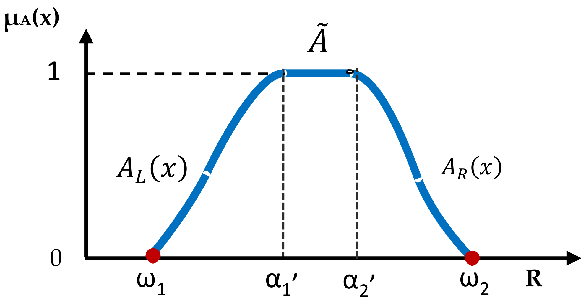
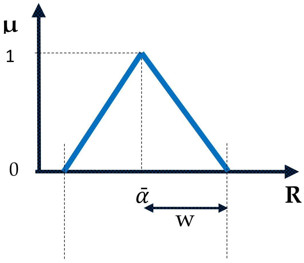
2.1. Principles of Fuzz Set and Logic

From a mathematical point of view, a fuzzy set can be described as a mapping from a general set X to the closed interval [0, 1] [31]. The membership function (MF) is a key concept which describes the fuzzy sets. Hence, the membership function declares to what degree an element belongs to the specific set. A membership degree of 0 denotes that the element does not belong to the set, and a membership degree of 1 denotes that the element belongs fully to the set. Subsequently, an element with a membership degree between 0 and 1 will partially belong to the examined set. A classical (crisp or precise or deterministic) set can be considered as a special case of a fuzzy set with a MF that only takes values 0 and 1.

A fuzzy number is a special case of the fuzzy set satisfying additionally the properties of convexity and normality. It is defined in the axis of real numbers, and its MF is a piecewise continuous function (Figure 1).

In general, the definition of fuzzy numbers can be found in Klir and Yuan, 1995. It is proven (Klir and Yuan, 1995) [31] that the MF of a fuzzy number (Figure 1) follows the mathematical expression (Equation (1)):

$${\mu }_A\left(x\right)=\left\{\begin{array}{l}0forx<{\omega }_1\\ A_L\left(x\right)for{\omega }_1\le x\le {\alpha }_1{}^{\prime }\\ 1for{\alpha }_1{}^{\prime }\le x\le {\alpha }_2{}^{\prime }\\ A_R\left(x\right)for{\alpha }_2{}^{\prime }\le x\le {\omega }_2\\ 0forx>{\omega }_2\end{array}\right.$$

(1)

where $A_L:\left[{\omega }_1,a_1{}^{\text{'}}\right]\to \left[0,1\right]$ and $A_R:\left[a_2{}^{\text{'}},{\omega }_2\right]\to \left[0,1\right]$ are the left and right parts of the membership function regarding the fuzzy number $\tilde{A}$. In addition, A_L is increasing and continuous from the right, and A_R is decreasing and continuous from the left. The interval [α₁′, α₂′] can be an interval or a point, but it cannot be an empty set [31].

A simple fuzzy number for representing the parameters K and x is the fuzzy symmetrical triangular number (Figure 2), which is a kind of fuzzy number [12]. The symbols $\overline{\alpha }, w$ denote the central value (a single point where μ = 1) and the width of the fuzzy number.

The h-cut set of the fuzzy number A (with 0 < h ≤ 1) is the key idea to move from the fuzzy to the precise (crisp) sets, and it is defined as follows [31,32] (Equation (2)):

$${\tilde{A}}_h=\left\{x\left|{\mu }_{\tilde{A}}\left(x\right)\ge h,x\in \Re \right.\right\}.$$

(2)

The h-cut set is a crisp set determined from the fuzzy set according to a selected value of the membership function, α, and, reciprocally, a fuzzy set can be derived from a significant number of α-cut sets. In the case of a fuzzy triangular number, the α-cut is (Equation (3)):

$${\tilde{A}}_h=\left[A_h^L,A_h^R\right]$$

or equivalently:

$${\tilde{A}}_h=\left[\overline{A}-\left(1-h\right)\cdot \left(\overline{A}-A_{}^{-}\right),\overline{A}+\left(1-h\right)\cdot \left(A_{}^{+}-\overline{A}\right)\right].$$

(3)

The crisp set including all the elements with non-zero membership function is the 0-strongcut, which is defined as follows [33,34] (Equation (4)):

$${\tilde{A}}_{0^{+}}=\left\{x\left|{\mu }_A\left(x\right)>0,x\in \Re \right.\right\}.$$

(4)

The following symbols are used for the zero-cut (Equation (5)):

$${\tilde{A}}_{0^{+}}=\left(A_{}^{-},A_{}^{+}\right).$$

(5)

More analytically, according to Equation (5), the 0-cut is an open interval and does not contain the boundaries. For this reason (and to have a closed interval containing the boundaries), Hanss (2005) [35] proposed the phrase “worst-case interval W”, which is the union of the 0-strongcut and the boundaries [35,36].

We can now extend the operation of the usual crisp functions in cases where the inputs are fuzzy sets, based on the extension principle that is briefly presented below.

Let X be a Cartesian product of universe $X=X_1\times X_2\times \dots \times X_n$ and ${\tilde{A}}_1,{\tilde{A}}_2,\dots ,{\tilde{A}}_n$ be defined in the universe sets $X_1,X_2,\dots ,X_n$, respectively. Let f be a (crisp) mapping from X to a universe Y, $y=f\left(x_1,x_2,\dots ,x_n\right)$. The mapping f for these particular input sets can now be defined as $\tilde{B}=\left\{\left(y,{\mu }_{\widetilde{{\rm B}}}\left(y\right)\right)\left|y=f\left(x_1,x_2,\dots ,x_n\right),\left(x_1,x_2,\dots ,x_n\right)\in X\right.\right\}$ in which the membership function of the image $\widetilde{{\rm B}}$ can be defined (Zimmermann 1991) [32] by (Equation (6)):

$${\mu }_{\tilde{B}}\left(y\right)=\underset{(x_1,x_2,\dots ,x_n)\in f^{-1}\left(y\right)}{\sup }\mathit{min}\left({\mu }_{A_n}\left(x_1\right),\dots ,{\mu }_{A_n}\left(x_n\right)\right)$$

(6)

where f⁻¹ is the inverse image of f.

The above principle is known as the extension principle. Its implementation provides the means to use a crisp function even if the inputs are fuzzy numbers. With most input variables, it is preferable to use a number of h-cuts in fuzzy analysis instead of using a MF based directly on the above definition ([37]). If f is a continuous function in the extension principle, the use of h-cuts can be also extended by determining the h-cuts of the function f, as follows ([33,34]) (Equation (7)):

$$\left\{\begin{array}{c}{f}^L{\left({\tilde{A}}_1,{\tilde{A}}_2,{\tilde{A}}_3\right)}_h=\mathit{min}\left\{f\left(x_1,x_2,x_3,h\right)\left|x_1\in {\tilde{A}}_{1h}\right.,x_2\in {\tilde{A}}_{2h},x_3\in {\tilde{A}}_{3h}\right\},\\ \\ f^R{\left({\tilde{A}}_1,{\tilde{A}}_2,{\tilde{A}}_3\right)}_h=\mathit{max}\left\{f\left(x_1,x_2,x_3,h\right)\left|x_1\in {\tilde{A}}_{1h}\right.,x_2\in {\tilde{A}}_{2h},x_3\in {\tilde{A}}_{3h}\right\}.\end{array}\right.$$

(7)

It is customary to use fuzzy numbers as inputs (here, the parameters K and x) to the crisp function (here, the Muskingum equation, which calculates the outflow, Q), and hence, the boundaries of the decision space will be closed (because of Equation (1)). Then, from the theorem of global existence for maxima and minima of functions with many variables, it is known that if the domain of a real function is closed and bounded, and the real function is continuous, then the function will have its absolute minimum and maximum values at some points in the domain [38]. Based on this theorem, in cases where fuzzy triangular numbers appear as inputs [37], the h-cut for any real continuous function with real variables in this domain can be determined. The determination of each h-cut is concluded to a double sub-optimization problem. Hence, the fuzzy output can be described by determining several representative h-cuts. Summarizing, in the case of fuzzy parameters, the simulation problem (that is, the determination of the outflow based on the Muskingum method) leads to the problem of determining several h-cuts, which is implemented through a double optimization procedure. In case of lateral flow, then a fuzzy estimation of the parameter α with the use of the h-cuts can be added.

2.2. Formulation of the Muskingum Method

The lumped hydrological model of Muskingum is based on the mass balance equation (Equation (8)) and the storage equation (Equation (9)).

$$I-Q=\frac{dS}{dt}$$

(8)

where I is the inflow rate to the reach, Q is the outflow rate from the reach, and S the storage in the reach. In the case where the relationship between storage and flow through a reach is linear, the Muskingum storage relationship can be written as (Equation (9)):

$$S=K\left[xI+\left(1-x\right)Q\right]$$

(9)

where I is the inflow rate to the reach, Q is the outflow rate from the reach, K is the storage time constant for the reach, and x is a weighting factor that varies between 0 and 0.5 [9].

The mass balance equation can be expressed in discrete form as follows (Equation (10)):

$$\frac{\left(I_j+I_{j-1}\right)}{2}\cdot \Delta t-\frac{\left(Q_j+Q_{j-1}\right)}{2}\cdot \Delta t=\left(S_j-S_{j-1}\right)$$

(10)

By combining Equations (8) and (9), the Muskingum routing equation is obtained (Equation (11)):

$$\begin{gathered} Q_j=C_0{I}_j+C_1{I}_{j-1}+C_2{Q}_{j-1} \\ \mathrm{where}{C}_0=\frac{-Kx+0.5\Delta t}{K-Kx+0.5\Delta t};C_1=\frac{\left(Kx+0.5\Delta t\right)}{K-Kx+0.5\Delta t};C_2=\frac{\left(K-Kx-0.5\Delta t\right)}{K-Kx+0.5\Delta t} \\ \mathrm{with}{C}_0+C_1+C_2=1 \end{gathered}$$

(11)

The linear Muskingum model can be modified to include the lateral flow. O’Donnell, 1985 [11] suggested a simple approach: “Possibly, the simplest model is one which assumes that the rate at which lateral inflow enters the reach is directly proportional to the rate of inflow I into the reach, with a proportionality factor α.”

Following this approach, the mass balance equation and the empirical storage equations can be written as (Equations (12) and (13)):

$$I\left(1+\alpha \right)-Q=\frac{dS}{dt}$$

(12)

$$S=K\left[x\left(1+\alpha \right)I+\left(1-x\right)Q\right]$$

(13)

After some algebraic operations, the following equation can be used (Equation (14)) [11]:

$$\begin{gathered} d_1{I}_j+d_2{I}_{j+1}+d_3{Q}_j=Q_{j+1}, \\ {d}_1=\left(1+\alpha \right)C_1,d_2=\left(1+\alpha \right)C_0,d_3=C_2 \end{gathered}$$

(14)

Or equivalently [12] (Equation (15)):

$$\begin{gathered} Q_j=\left(1+a\right)\frac{\Delta {\rm T}+2Kx}{\Delta {\rm T}+2K\left(1-x\right)}{I}_{j-1}+\left(1+a\right)\frac{\Delta {\rm T}-2Kx}{\Delta {\rm T}+2K\left(1-x\right)}{I}_j \\ +\frac{-\Delta {\rm T}+2K\left(1-x\right)}{\Delta {\rm T}+2K\left(1-x\right)}{Q}_{j-1} \end{gathered}$$

(15)

The focus of this work is the crisp function that determines the current outflow when the parameters K and x are fuzzy numbers. Whereas in the case of no lateral flow, the Equation (11) describes this function, in the case of lateral flow, the Equation (15) is applied.

2.3. Implementation of the Muskingum Method with Fuzzy Parameters

In this study, the parameters K and x (and α in case of lateral flow) are selected by assuming them as fuzzy triangular symmetrical numbers (Figure 2). The simple linear Muskingum equation is applied with fuzzy parameters. As aforementioned, the application of a crisp function with fuzzy parameters is achieved by applying the extension principle. In practice, several h-cuts can be determined in order to describe the values of the examined function (in this application, the function $f$ describes the outflow). In case of no lateral flow (based on Equation (11)), the boundaries of each h-cut of the outflow can be determined as follows (Equation (16)):

$$\left\{\begin{array}{c}{Q}_j{}^L{\left(\tilde{K},\tilde{x}\right)}_h=\mathit{min}\left\{\begin{array}{c}\frac{\Delta {\rm T}+2x_1{x}_2}{\Delta {\rm T}+2x_1\left(1-x_2\right)}{I}_{j-1}+\frac{\Delta {\rm T}-2x_1{x}_2}{\Delta {\rm T}+2x_1\left(1-x_2\right)}{I}_j+\\ \frac{-\Delta {\rm T}+2x_1\left(1-x_2\right)}{\Delta {\rm T}+2x_1\left(1-x_2\right)}{Q}_{j-1}\left|x_1\in {\tilde{K}}_h\right.,x_2\in {\tilde{x}}_h\end{array}\right\},\\ Q_j{}^R{\left(\tilde{K},\tilde{x}\right)}_h=\mathit{max}\left\{\begin{array}{c}\frac{\Delta {\rm T}+2x_1{x}_2}{\Delta {\rm T}+2x_1\left(1-x_2\right)}{I}_{j-1}+\frac{\Delta {\rm T}-2x_1{x}_2}{\Delta {\rm T}+2x_1\left(1-x_2\right)}{I}_j+\\ \frac{-\Delta {\rm T}+2x_1\left(1-x_2\right)}{\Delta {\rm T}+2x_1\left(1-x_2\right)}{Q}_{j-1}\left|x_1\in {\tilde{K}}_h\right.,x_2\in {\tilde{x}}_h\end{array}\right\},\end{array}\right.$$

(16)

where I is the inflow rate to the reach, Q is the outflow rate from the reach, K is the storage time constant for the reach, and x is a weighting factor. The index j is referred to the time step, and the indexes L and R are referred to the left and the right hand of the produced h-cut regarding the examined fuzzy number.

In cases of lateral flow, based on Equation (15) it holds (Equation (17)):

$$\begin{array}{c}{Q}_j{}^L{\left(\tilde{K},\tilde{x},\tilde{a}\right)}_h=\mathit{min}\left\{\begin{array}{c}\left(1+x_3\right)\frac{\mathsf{\Delta }{\rm T}+2x_1{x}_2}{\mathsf{\Delta }{\rm T}+2x_1\left(1-x_2\right)}{I}_{j-1}+\left(1+x_3\right)\frac{\mathsf{\Delta }{\rm T}-2x_1{x}_2}{\mathsf{\Delta }{\rm T}+2x_1\left(1-x_2\right)}{I}_j\\ +\frac{-\mathsf{\Delta }{\rm T}+2x_1\left(1-x_2\right)}{\mathsf{\Delta }{\rm T}+2x_1\left(1-x_2\right)}{Q}_{j-1}\left|x_1\in {\tilde{K}}_h\right.,x_2\in {\tilde{x}}_h,x_3\in {\tilde{a}}_h\end{array}\right\},\\ Q_j{}^R{\left(\tilde{K},\tilde{x},\tilde{a}\right)}_h=\mathit{max}\left\{\begin{array}{c}\left(1+x_3\right)\frac{\mathsf{\Delta }{\rm T}+2x_1{x}_2}{\mathsf{\Delta }{\rm T}+2x_1\left(1-x_2\right)}{I}_{j-1}+\left(1+x_3\right)\frac{\mathsf{\Delta }{\rm T}-2x_1{x}_2}{\mathsf{\Delta }{\rm T}+2x_1\left(1-x_2\right)}{I}_j\\ +\frac{-\mathsf{\Delta }{\rm T}+2x_1\left(1-x_2\right)}{\mathsf{\Delta }{\rm T}+2x_1\left(1-x_2\right)}{Q}_{j-1}\left|x_1\in {\tilde{K}}_h\right.,x_2\in {\tilde{x}}_h,x_3\in {\tilde{a}}_h\end{array}\right\},\end{array}$$

(17)

For the case of non-lateral flow, to calibrate the Muskingum method, the parameters K and x need to be estimated. The central values (h = 1) and the left and the right hands of the zero-cut (or the worst-case interval W) regarding the outflow are exploited. The zero-cut can be used to express the concept of inclusion, that is, to check the property that the fuzzy band contains the observed data at least to a high degree. This is set as a key idea in order to calibrate the proposed fuzzy Muskingum model. The determination of the boundaries of the worst-case interval W is finally achieved by following an optimization procedure, which, in the examined case, will have a solution since the inputs are fuzzy numbers and the used crisp function Q is continuous. The determination of the worst-case interval W composes the sub-optimization problem that arises during the calibration of the model.

The problem of the calibration process is to assess the central values and the semi-width of the parameters K, x, and α so that a selected criterion is minimized (including the inclusion constraints). Because of the model complexity, the calibration is achieved by applying a heuristic optimization model. In this article, the particle swarm optimization (PSO) method is selected. This method can be coupled with a simulation model; in this study, the Muskingum equation enhanced with the use of the extension principle for fuzzy parameters is applied.

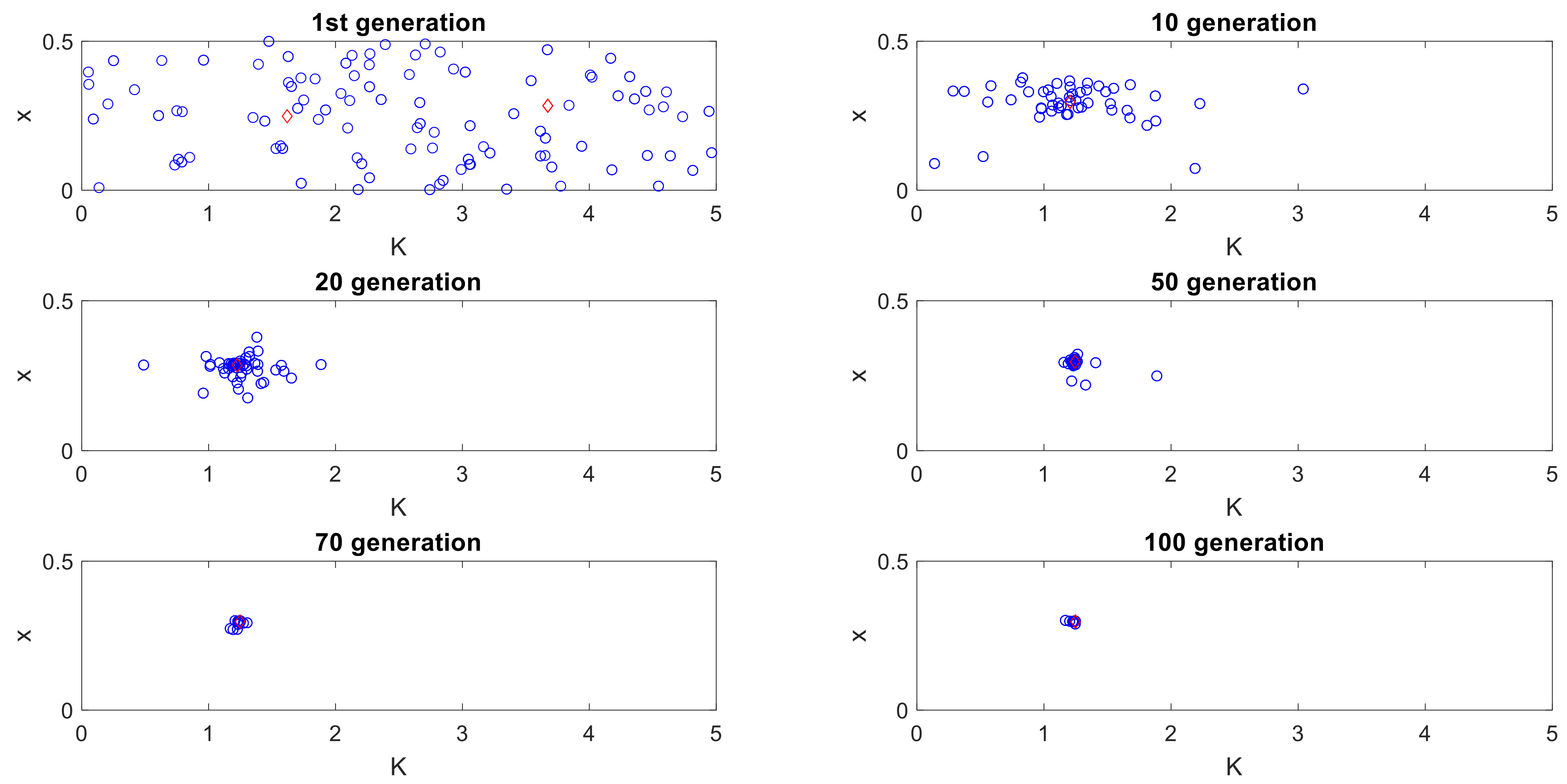
2.4. Particle Swarm Optimization Method

Particle swarm optimization (PSO) is a stochastic global optimization method based on the simulation of the swarm. As in genetic algorithms (GA), PSO exploits a population of possible candidate solutions to probe the search area. The PSO algorithm can be characterized as one of the population-based algorithms (Parsopoulos and Vrahatis, 2002) [39]. Although PSO is an effective and widely used method, it is simpler than other heuristic optimization algorithms (e.g., GA) because the crossover and mutation operations in the original version of the GA [40,41] are not used.

PSO can deal with nonlinear optimization problems in non-convex domains [42]. Each candidate solution is called a particle, and the set of potential possible solutions in each iteration creates the swarm [41,43]. A swarm has a dimension N′, in which N′ is the number of potential solutions. Each potential solution is comprised of D variables, in which D is the dimension of the problem [41,44]. In this article, in case of non-lateral flow, D = 4 $\left(\overline{K},w_K,\overline{x},w_x\right)$, where $\overline{K}$is the central value of $\tilde{K}$, $w_K$ the semi-width of $\tilde{K}$, $\overline{x}$ is the central value of $\tilde{x},w_x$is the semi-width of $\tilde{x}$.

Analytically, the population dynamics in PSO simulates the behavior of a bird flock, where social sharing of information takes place and individuals benefit from the discoveries and previous experience of all other companions during their search for food. Thus, two variants of the PSO algorithm were developed considering either a local neighborhood or a global neighborhood. In the former, the partial optimum of the particle is usually applied [40]. In the latter, each particle moves towards its best previous position and towards the best particle in the whole swarm [39,41,45].

Several modifications to the original version of the PSO method of Kennedy and Eberhart (1995) [45] have been proposed, such as the adaptation of inertia term and the consideration of the maximum velocity (e.g., [46]).

The basic PSO algorithm is detailed below (e.g., [44,46,47]:

1:

Initialize a population array of particles with random positions and velocities on D dimensions in the search area.

2:

Loop

3:

For each particle, evaluate the desired optimization fitness function in D variables.

4:

Compare particle fitness evaluation with its best previously visited position (p_i). If the current value is better than p_i, then set p_i equal to the current value.

5:

Identify the particle with the best fitness function value of the swarm p_g.

6:

Change the velocity and position of the particle (x_i) according to the Equation (18):

$$\left\{\begin{array}{l}{\upsilon }_i\left(t+1\right)=\omega {\upsilon }_i+c_1{\rho }_1\cdot \left(p_i-x_i\left(t\right)\right)+c_2{\rho }_2\cdot \left(p_g-x_i\left(t\right)\right)\\ x_i\left(t+1\right)=x_i\left(t\right)+{\upsilon }_i\left(t+1\right)\end{array}\right.$$

(18)

7:

If a criterion is met (usually a sufficiently good fitness or a maximum number of iterations), exit loop.

8:

End loop

where ρ() is a vector of random numbers uniformly distributed in the open interval 0, 1 that is generated at each iteration, and for each particle, p_i is the best previously visited position of the ith particle (partial optimum), and $p_g$ is the global best previously visited position of all particles (global optimum). Furthermore, the term $c_1{\rho }_1\cdot \left({\overrightarrow{p}}_i-{\overrightarrow{x}}_i\right)$that associates the particle’s own experience with its current position is weighted by the constant $c_1$ and is called individuality (cognitive acceleration). The term $c_2{\rho }_2\cdot \left({\overrightarrow{p}}_g-{\overrightarrow{x}}_i\right)$is associated with the social interaction between the particles of the swarm and weighted by the constant $c_2,$ and is called sociality (social acceleration). As υ the velocity is meant. The velocity, by supposing that Δt = 1, modulates the new position $x_i\left(t+1\right).$

For the basic PSO, the coefficients $c_1$ and $c_2$ were allowed to take values in the interval 1.5 to 2.5 [41].

Clerc and Kennedy’s analysis [48] based on the initial PSO method proposed the following modified equation for the new positions (Equation (19)):

$$\left\{\begin{array}{l}{\upsilon }_i\left(t+1\right)=\chi \left[{\upsilon }_i\left(t\right)+c_1{\rho }_1\cdot \left(p_i-x_i\left(t\right)\right)+c_2{\rho }_2\cdot \left(p_g-x_i\left(t\right)\right)\right]\\ x_i\left(t+1\right)=x_i\left(t\right)+{\upsilon }_i\left(t+1\right)\end{array}\right.$$

(19)

where χ is a parameter called constriction coefficient or constriction factor (Equation (20)):

$$\chi =\frac{2}{\left|2-\phi -\sqrt{{\phi }^2-4\phi }\right|},\phi =c_1+c_2,\phi >4$$

(20)

On the other hand, based on the literature, the following parameters are proposed ([48]) (Equation (21)):

$$\chi =0.729,c_1=c_2=2.05$$

(21)

In this study, the proposals of Clerc & Kennedy, 2002 are adopted in the implementation of the PSO.

It is worth noting that, in some cases, the PSO method converges rapidly to a local optimum. This problem can be overcome by the strategy of Salehizadeh et al. (2009) [49] by dividing the population or by using other hybrid methods, e.g., by combining the PSO together with simulated annealing behavior. For instance, [41] applied a modified PSO to achieve the identification of optimal hedging rules for complex real systems of operating reservoirs with many parameters, seeking to mitigate the drought impacts.

3. Proposed Calibration and Performance Measures

A procedure is followed to implement the model calibration (PSO) method together with the extension principle. First, a swarm of possible solutions is randomly created within the decision space. For non-lateral flow, each possible optimum solution (member of the swarm) contains the values of the parameters $\left(\overline{K},\overline{x},w_K,w_x\right)$ that describe the membership functions of $\tilde{K},\tilde{x}$. Then, a fuzzy simulation method is applied based on the extension principle. For each possible solution, the frontiers of the 0-cut and the central values are calculated. Finally, we apply the PSO methodology, and the objective is calculated. The objective function is identical with the fitness function, since by using the simulation stage, the use of constraints could be avoided.

The key question is about the formulation of the objective function (fitness function), which will be used during the calibration process. The objective function will differ from those selected by the crisp calibrations, since the output of the model will be a fuzzy band that expresses the outflow hydrograph. In this article, an objective function that contains a weighted sum of four performance measures is proposed (Equations (22)–(24)):

$$\begin{array}{l}f=w_1\underset{includingalldata}{\left[{\displaystyle \sum _{j=1}^M{a}_{R_j}{\left(Q_j^{observed}-Q_j^{+}\right)}^2}+{\displaystyle \sum _{j=1}^M{a}_{L_j}{\left(Q_j^{-}-Q_j^{observed}\right)}^2}\right]}+\underset{centralvaluesneartodata}{\frac{1}{M}\left({\displaystyle \sum _{j=1}^M{\left(Q_j^{observed}-{\overline{Q}}_j^{}\right)}^2}\right)}+\\ \frac{1}{M}\underset{fuzzywidth}{\left({\displaystyle \sum _{j=1}^M{\left(Q_j^{+}-Q_j^{-}\right)}^2}\right)}+\underset{includingthemaximumvalue}{\left(a_{\mathit{max}}{\left(Q_{}^{\mathit{max}}-Q_p^{+}\right)}^2\right)}\end{array}$$

(22)

where

$$a_{R_j}=\left\{\begin{array}{c}0 if Q_j^{+}\ge Q_j^{observed}\\ 1 if Q_j^{+}\le Q_j^{observed}\end{array}\right., a_{L_j}=\left\{\begin{array}{c}0 if Q_j^{-}\le Q_j^{observed}\\ 1 if Q_j^{-}\ge Q_j^{observed}\end{array}\right.$$

(23)

The first term expresses the divergence of the produced fuzzy band to include all data. In other words, the squared penalty term, E₁, is activated only whether the observed data are not included within the produced fuzzy band. This procedure was initially proposed by Ishibuchi et al. (1993) [50] as a cost function to be minimized in the learning process regarding a neural network with interval weights, whilst in this work, it is used as a term of the fitness function (Equation (24)):

$$E_1=\underset{}{\left[\sum _{j=1}^M{a}_{R_j}{\left(Q_j^{observed}-Q_j^{+}\right)}^2+\sum _{j=1}^M{a}_{L_j}{\left(Q_j^{-}-Q_j^{observed}\right)}^2\right]}{\left(\frac{m^3}{s}\right)}^2$$

(24)

The above measure represents the idea of inclusion of the fuzzy linear regression of Tanaka [30]. According to this model, all the data must be included within the produced fuzzy band [51,52].

The second term, E₂, expresses the distance between the central values (α = 1) and the observed data (Equation (25)):

$$E_2=\underset{}{\left(\sum _{j=1}^M{\left(Q_j^{observed}-{\overline{Q}}_j\right)}^2\right)}{\left(\frac{m^3}{s}\right)}^2$$

(25)

The third term, E₃, expresses the magnitude of the produced fuzzy width. A large width leads to an unfunctional fuzzy band, which cannot be exploited in real applications (Equation (26)):

$$E_3=\underset{}{\left(\sum _{j=1}^M{\left(Q_j^{+}-Q_j^{-}\right)}^2\right)}{\left(\frac{m^3}{s}\right)}^2$$

(26)

The use of this distance comes from the fuzzy regression of Tanaka where the problem of the fuzzy linear regression concludes to a constrained optimization problem aiming to minimize the total width of the produced fuzzy band (e.g., [51,52])

Finally, the last term, E₄, expresses the distance between the maximum value of the outflow and the right hand of the estimated outflow (Equations (27) and (28)):

$$E_4=\underset{includingthemaximumvalue}{\left(a_{\mathit{max}}{\left(Q_{}^{\mathit{max}}-Q_p^{+}\right)}^2\right)}{\left(\frac{m^3}{s}\right)}^2$$

(27)

$$\mathrm{where}{a}_{\mathit{max}}=\left\{\begin{array}{l}1if{q}_{}^{\mathit{max}}\ge q_p^{+}\\ 0otherwise\end{array}\right.,p:timewhen{q}_{\mathit{max}}=\mathit{max}(Q_1,\dots ,Q_j,\dots ,Q_M)$$

(28)

This distance is activated only if the observed data are above the produced fuzzy band as it is indicated by the coefficient α_max where p is the time, which is referred to as the time where the maximum value occurs. This criterion is useful in river routing. For flood protection, it is critical that the produced fuzzy band (from the proposed model) includes the observed maximum value even in real time. Therefore, since this criterion expresses the aforementioned property, it is obviously useful. This measure is proposed by [44] where a fuzzified version of the fuzzy unit hydrograph was developed.

The terms $Q_j^{observed},Q_j^{-} , \mathrm{and} Q_j^{+}$express the observed value at time j, the left, and the right-hand boundary of the zero-cut, respectively.

These behavioral parameters are user defined and control the optimization process. The adopted values were taken mainly from the literature because they are shown to lead to good performance. Their effectiveness is later analyzed and compared to other alternatives in the validation section.

The weight w₁ is selected to give more emphasis on the first term of the fitness function. Indeed, the main advantage of the fuzzy model, similarly with the fuzzy regression model (e.g., [30]), is the inclusion of the observed data into the produced fuzzy band. However, in the case of a precise satisfaction of the inclusion constraints, then an outlier can significantly enlarge the size of the produced fuzzy band. Hence, the larger the w₁, the closer to the absolute satisfaction of the inclusion constraints the model becomes. If a non-useful fuzzy band is produced, then the value of w₁ is reduced. In fact, the first measure strengthens the satisfaction of the inclusion constraints. E₁ conflicts with E₃; however, an unfunctional fuzzy band must be rejected. E₂ is similar but not identical with the crisp measures SSQ, since apart from the central value, the output of the fuzzy model is the entire fuzzy number.

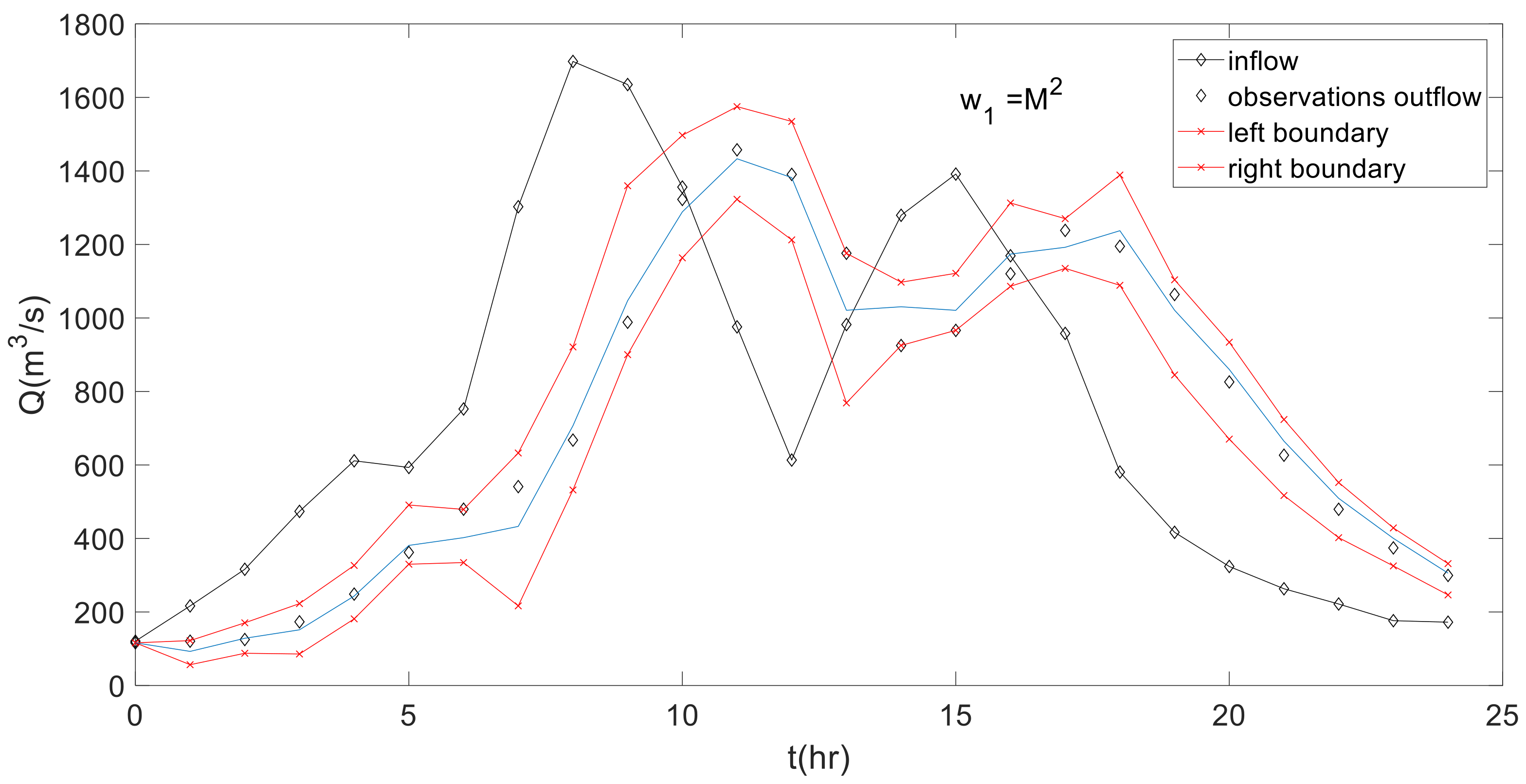
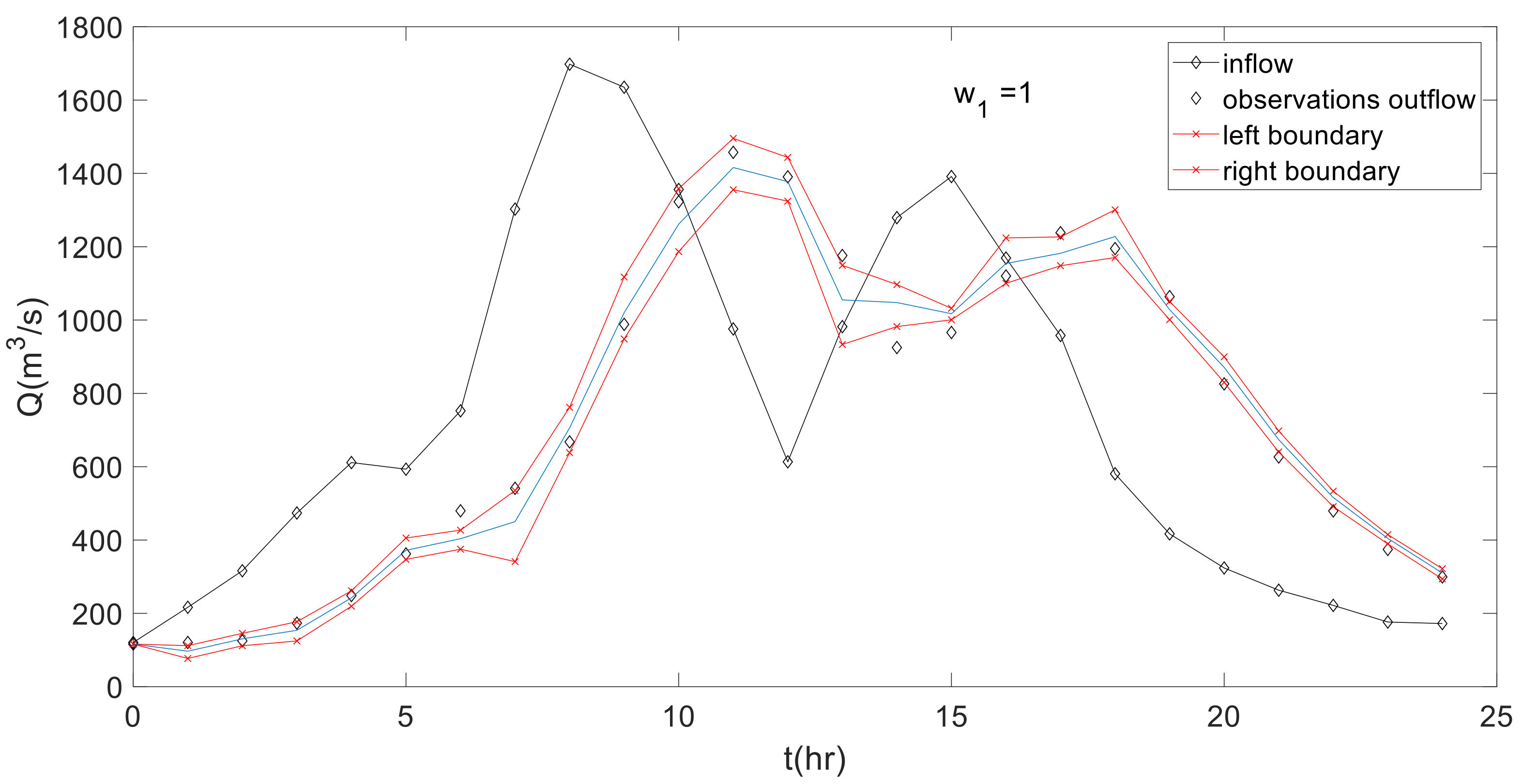
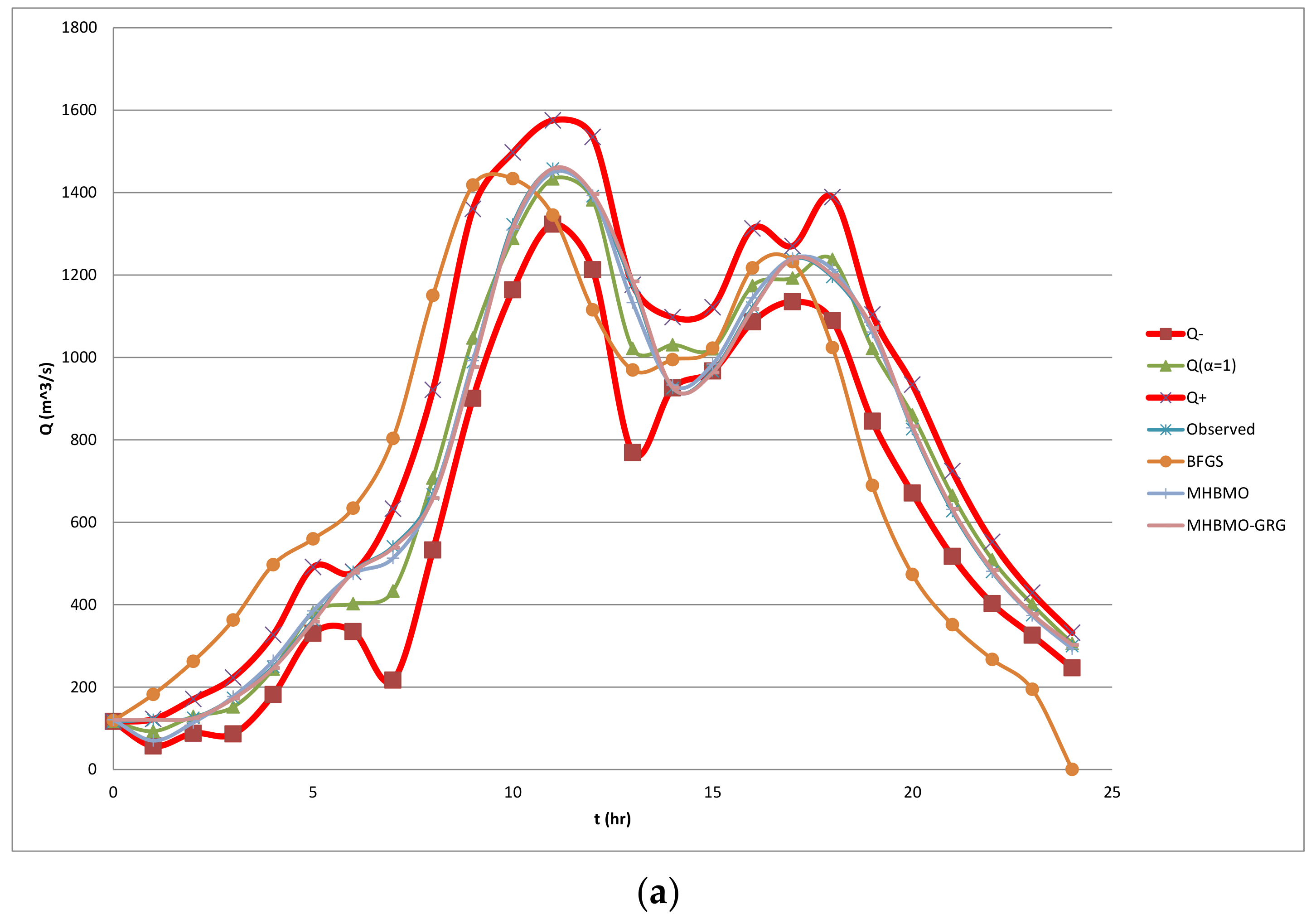
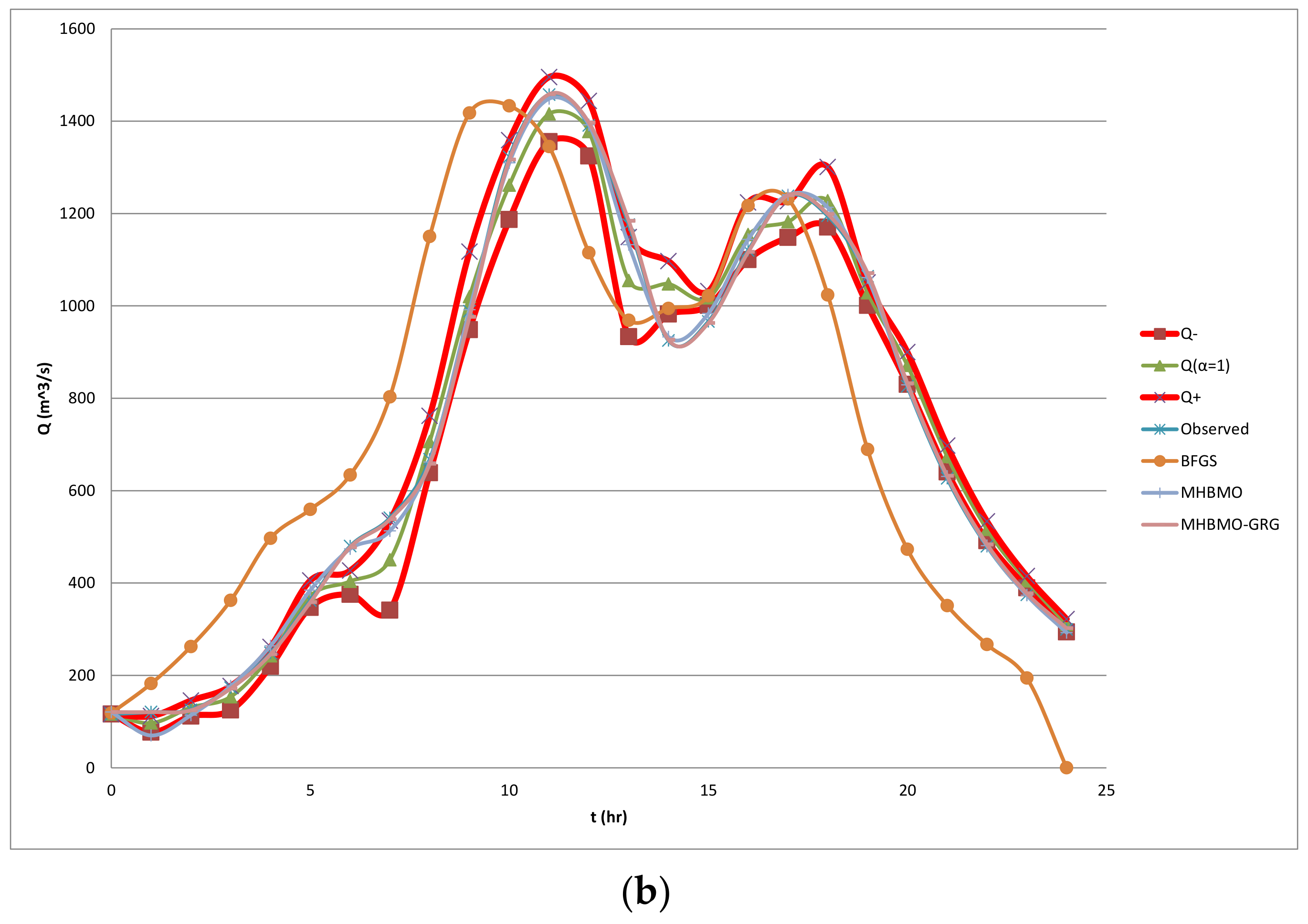
4. Results and Discussion

In order to check the proposed methodology, four case studies from the references are used to benchmark the proposed method. The first three case studies include: (1) the routing of a smooth hydrograph (Wilson 1974 [10]), (2) a double peak hydrograph (Viessman and Lewis 2003 [9]), and (3) non-smooth hydrograph with lateral flow (O’Donnel 1985) data sets [11]. The last case study is located in the Ebro River Basin with more data available. Therefore, the validation of the solution achieved is studied in the last case study.

4.1. Smooth Hydrograph

The first data set is the data set presented by [10]. For these kinds of heuristic optimization problems, a maximum of 100 iterations were selected. Furthermore, the swarm consists of 50 members, whilst the expression of Clerc and Kennedy’s is adopted for training (Equations (19)–(21)). The results were not practically changed even if the SWARM was activated again. The fitness or objective function consists of the four performance measures (Equation (22)). These selections were adopted for all the examined examples.

Since no lateral flow occurs, the Equation (16) is used to determine the boundary of the worst-case interval W, which is used to check the width of the produced fuzzy band and the degree of inclusion. Because of the sub-optimization problems (according to extension principle, Equation (16)) a significant computational time is required for the calibration process. Initially, a significant value of the w₁ is considered (w₁ = M²). By following the aforementioned calibration procedure, the following results are achieved:

$$\tilde{K}=\left(1.2482,0.6533\right)\mathrm{days}\mathrm{and} \tilde{x}=\left(0.2972,0.0580\right)\mathrm{and}{E}_1=3.31$$

where M is the number of data, whilst in the bracket, the first term means the central value and the second term the semi-width. The brackets symbolize the fuzzy symmetrical triangular numbers.

Wilson, 1974 [10] proposed the following crisp values for the examined parameters: K = 1.5 days and x = 0.25, which are included from the produced corresponding quantities.

Therefore, the produced solution has physical sense and incorporates all the data to a high degree. However, the above suggestion holds only if the width of the produced fuzzy band is functional. For flood protection, the most important factor is the uncertainty within the neighborhood of the peak flow. Figure 3 shows that a range between the left and the right boundaries of the outflow is lower than 10 m³/s, which seems a reasonable range. However, the greater values have a high dispersion in time according to the proposed fuzzy solution.

The crisp formulation uses the measure $SSQ={\sum }_{j=1}^M{\left(Q_j^{observed}-Q_j\right)}^2,$ which cannot be compared directly with the performance evaluation measures, since according to the proposed methodology, the output of the fuzzy Muskingum simulation will be a fuzzy number in contrast with the crisp formulation where the output is a crisp number. In case a significantly very small weight w₁ is selected, an almost crisp solution is obtained. In this case, the value of E₁, E₂, and SSQ are practically identical. However, the comparison between the SSQ and E₁ indicates that E₁ takes the smallest value (

Table 1. The logical test that is true if the fuzzy solution contains the other crisp methods. P (green box) means that the model “passed” the test, and F (red box) means that the model “failed”.

	Time (Hours)
Models	0	6	12	18	24	30	36	42	48	54	60	66	72	78	84	90	96	102	108	114	120	126
Wilson-trial	P	P	P	P	P	P	P	P	P	P	P	P	P	P	P	P	P	P	P	P	P	P
Regression	P	P	P	P	P	P	P	P	P	P	P	P	P	P	P	P	P	F	F	F	F	F
NL-LSM	P	P	F	F	P	P	P	P	P	P	P	P	P	P	F	P	P	P	P	F	F	F
S-LSM	P	P	F	F	P	P	P	P	P	P	P	P	P	P	P	P	P	P	F	F	F	F
LMM	P	P	F	F	P	P	P	P	P	P	P	P	P	P	P	P	P	P	F	F	F	F
HJ+DFP	P	P	P	P	P	P	P	P	P	P	P	P	P	P	P	P	P	P	P	P	P	P
GA	P	P	P	P	P	P	P	P	P	P	P	P	P	P	P	P	P	P	P	P	P	P
BFGS	P	P	P	P	P	P	P	P	P	P	F	P	P	P	P	P	P	P	P	P	P	P
BFGS-HS	P	P	P	P	P	P	P	P	P	P	F	P	P	P	P	P	P	P	P	P	P	P
NLMM-L	P	P	P	P	P	P	P	P	P	P	P	P	P	P	P	P	P	P	P	F	F	F
NLI (SSQ)	P	P	P	P	P	P	P	P	P	P	P	P	P	P	P	P	P	P	P	P	F	F
NLII (SSQ)	P	P	P	P	P	P	P	P	P	P	P	P	P	P	P	P	P	P	P	P	P	P
NLIII (SSQ)	P	P	P	P	P	P	P	P	P	P	P	P	P	P	P	P	P	P	P	P	P	F
NLI (MARE)	P	P	P	P	P	P	P	P	P	F	P	P	P	P	P	P	P	P	P	P	P	P
NLII (MARE)	P	P	P	P	P	P	P	P	P	F	P	P	P	P	P	P	P	P	P	P	P	P
NLIII (MARE)	P	P	P	P	P	P	P	P	P	F	P	P	P	P	P	P	P	P	P	P	P	F

in Niazkar and Afzali, 2016) of the SSQ.

To summarize, it is proposed that, in the case E₁ has a small value (preferably smaller than the SSQ of the crisp simulation) and a logical width, then the fuzzy calibration can be accepted. The time-step of Wilson 1974 [10], 6 h, can be characterized as sufficient, since in 6 h, some emergency measures can be implemented.

Analytically, for w₁ = M², the proposed measures, for which their weighted sum composes the objective function, have the following values:

$$\begin{array}{l}{E}_1=\underset{includingalldata}{\left[{\displaystyle \sum _{j=1}^M{a}_{R_j}{\left(Q_j^{observed}-Q_j^{+}\right)}^2}+{\displaystyle \sum _{j=1}^M{a}_{L_j}{\left(Q_j^{-}-Q_j^{observed}\right)}^2}\right]}=3.31\\ E_2=\underset{centralvaluesneartodata}{\left({\displaystyle \sum _{j=1}^M{\left(Q_j^{observed}-{\overline{Q}}_j^{}\right)}^2}\right)}=344.9\\ \underset{fuzzywidth}{E_3=\left({\displaystyle \sum _{j=1}^M{\left(Q_j^{+}-Q_j^{-}\right)}^2}\right)}=\mathrm{3,410.8}\\ E_4=\underset{includingthemaximumvalue}{\left(a_{\mathit{max}}{\left(Q_{}^{\mathit{max}}-Q_p^{+}\right)}^2\right)}=0.02\end{array}$$

Two additional calibrations are presented in Figure 4 for (a) w₁ = 1 and (b) w₁ = 1/M. In cases where smaller weights are selected, the produced fuzzy band becomes thinner and smoother (Figure 4a,b), but it cannot contain a significant number of data (especially Figure 4b, where a smaller weight is selected). However, the maximum discharge is practically included in all cases. In all figures, the blue line expresses the central value, that is, the value which corresponds to unit membership function.

For illustrative purposes, Figure 5 shows the evolution of the member of the swarm. Since there are four decision variables, only the parameters central values of K and x are represented. The blue circles indicate the swarm of the possible solutions and the diamond the global optimum solution for each generation. After the 50th generation, the swarm converts rapidly near the global optimum, and the optimum solution remains stable after the 89th iteration.

After the end of the calibration procedure (and hence, the PSO algorithm), for each time step, the fuzzy number which corresponds to the outflow can be separately calculated by considering a very large number of h-cuts. For each h-cut, the extension principle is used to determine the boundaries of each h-cut. Figure 6 represents the produced outflow when the maximum outflow occurs in the observed data. As it can be seen, the output remains a fuzzy number (since it satisfies Equation (1)), but the linearity and the symmetry (which appears in case of the parameters K and x) were lost because the used crisp functions (Equation (16)) do not remain linear.

By comparing the proposed fuzzy solution with many (crisp) methodologies, it is concluded that the fuzzy solution contains the majority of the described solutions (see the literature session). Indicatively, the Wilson-trial approach [10], the regression model, the NL-LSM (Yoon and Padmanabhan 1993) [15], the S-LSM (Gill 1978) [13], the LMM (Das 2004) [7], the HJ+DFP (Tung 1985) [14], the GA, the BFGS (Geem 2006) [16], the BFGS-HS (Karahan et al., 2013), the NLMM-L (Karahan et al., 2013), the NLI (SSQ) (Karahan et al., 2013), the NLII (SSQ) (Karahan et al., 2013), the NLIII (SSQ) (Karahan et al., 2013), the NLI (MARE) (Karahan et al., 2013), the NLII (MARE) (Karahan et al., 2013), the NLIII (MARE) (Karahan et al., 2013) [53], the CS (Karahan et al., 2015) [18], and the CM (Easa 2015) [26] models are figured together with the fuzzy solution. The fuzzy solution is depicted by the left-hand and the right-hand bound of the zero-cut and the central values (Figure 7).

The Table 1 contains the comparison between the fuzzy solution with the aforementioned crisp models. The logical test is passed when the previous crisp solution for the outflow is included within the produced fuzzy band. A tolerance of 1 m³/s is permitted. From Table 1, it is shown that the majority of the crisp solutions are included within the produced fuzzy band apart from the last (decreasing) part of the hydrograph. The yellow lines indicate the time steps near the time where the maximum occurs.

In addition, the produced fuzzy band is separately compared with the graphical solution of Wilson, 1974 [10] (Figure 8). The graphical solution is based on the graphical representation of the storage versus the weighted discharge and with x as the preferred value, which produces the narrowest loop. An important point is that by comparing the central values of the fuzzy solution and the graphical solution, these two solutions are close, and moreover, the initial region of the outflows has a similar decreasing behavior.

4.2. Two-Peak Hydrograph

The second case study is a multi-peak flood hydrograph [9]. By selecting $w_1=M^2$ $, \tilde{K}=\left(3.5744,1.5672\right), \mathrm{and}\tilde{x}=\left(0.3460,0.1399\right)$, whilst$E_1=0.51$ (Figure 9), where M is the number of data for the examined set.

By selecting $w_1=1,$ a functional approach with a smaller fuzzy band but with some points out of the fuzzy band is produced (Figure 10). The value E₁ = 8974.5, which is sufficient. $\tilde{K}=\left(3.6975,0.3954\right) \mathrm{hr}\mathrm{and} \tilde{x}=\left(0.3134,0.1067\right)$. An interesting perspective is that the two solutions are very close regarding the central values.

Furthermore, the produced fuzzy band is compared with BFGS (Karahan 2014) [54] and MHBMO (Niazkar and Afzali 2015) [25] (Figure 11). Although the crisp models are rather complex with many parameters, the fuzzy model based on the Muskingum linear method contains practically all the values for w₁ = M² (Figure 11a) and the majority of the values when w₁ = 1 (Figure 11b), whilst the fuzziness is within a rational value. The method of BFGS seems to be away from the data.

4.3. Non-Smooth Hydrograph with Lateral Flow

A non-smooth outflow hydrograph with lateral flow, previously presented by O’Donnel (1985) [11], was analyzed. The data are based on the event on the River Wyre, 20–21 October 1982. The river flows into the Irish Sea at Fleetwood. It is approximately 28 miles (45 km) in length. The river is a county Biological Heritage Site. According to O’ Donnel (1985), there was a considerable increase in the flood volume between the inflow and outflow sections (some 25 km apart), and furthermore, it also had a multi-peaked inflow. Initially, a significant value of the w₁ is considered (w₁ = M²). Since lateral flow occurs, Equation (17) is used to determine the worst-case interval. By selecting $w_1=M^2$, it is concluded that $\tilde{K}=\left(4.9405,2.1945\right), \tilde{x}=\left(0.0593,0.1035\right),\mathrm{and} \tilde{a}=\left(2.5960,0.1035\right)$ (Figure 12). However, the values of x approach the value corresponding to the reservoir, whilst small negative values are expected to be irrational.

By selecting $w_1=1,$ (Figure 13) it is concluded that $\tilde{K}=\left(6.7211,2.6006\right), \tilde{x}=\left(0.0997, 0.0002\right), \mathrm{and}\widetilde{ a}=\left(2.9648,0.1848\right)$ and E = 23.4438. These values approximate the crisp values that are provided by [11]. By comparing the observed data and the produced fuzzy band, it seems that although a new parameter was added, the performance of the fuzzy solution can be characterized as sufficient since the produced fuzzy band includes to a high degree the observed data of the outflow without an irrational width.

Based on the three examples analyzed, results show advantages of the proposed methodology to be highlighted: (1) the use of a fuzzy estimation with the aim of fuzzy parameters is closer to observed; (2) the new methodology increases the safety of the prediction including the uncertainty; (3) the produced fuzzy band include, to a significant degree, the observed data; and (4) the output of the successful existent crisp methodologies even if they include more complex assumptions.

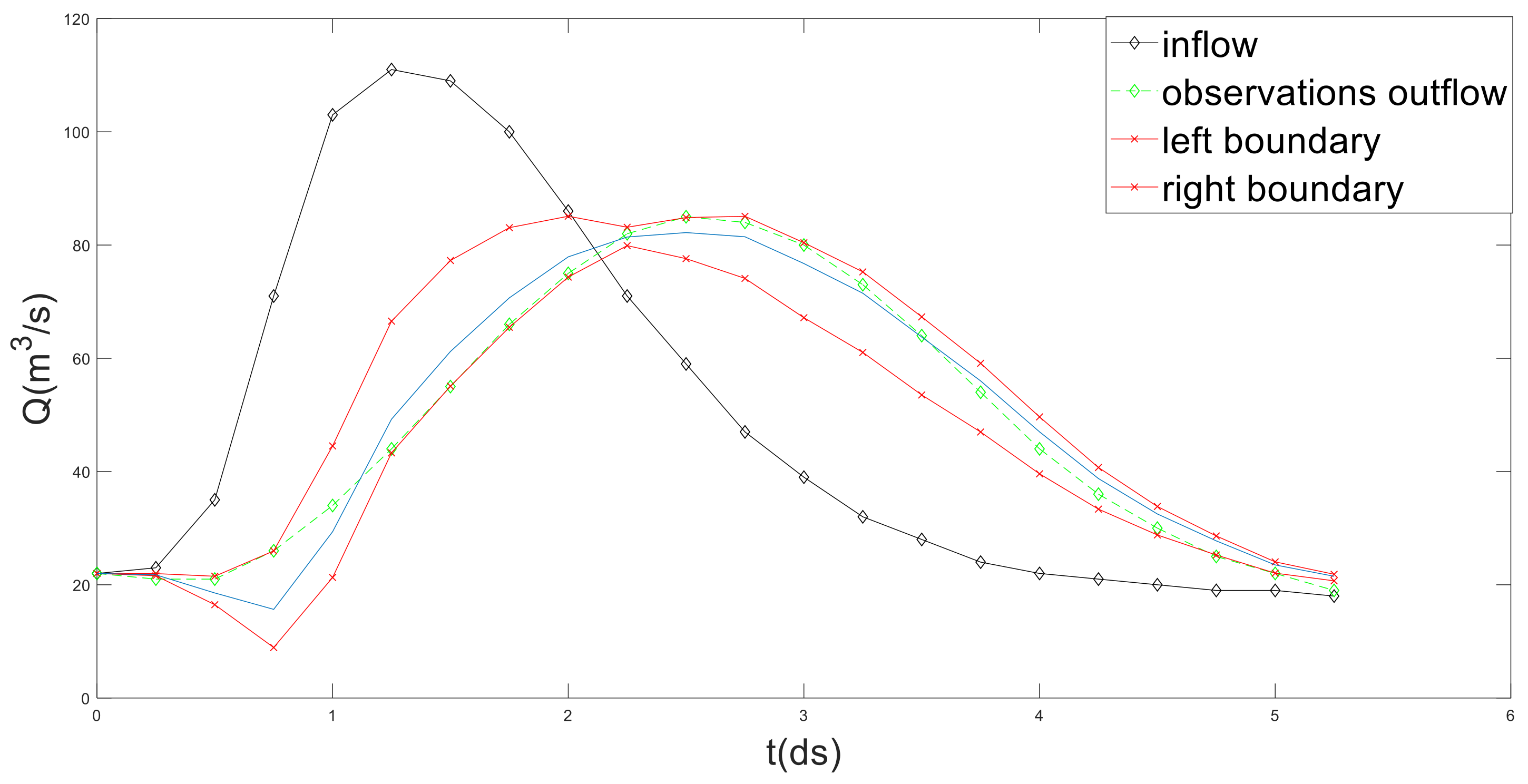
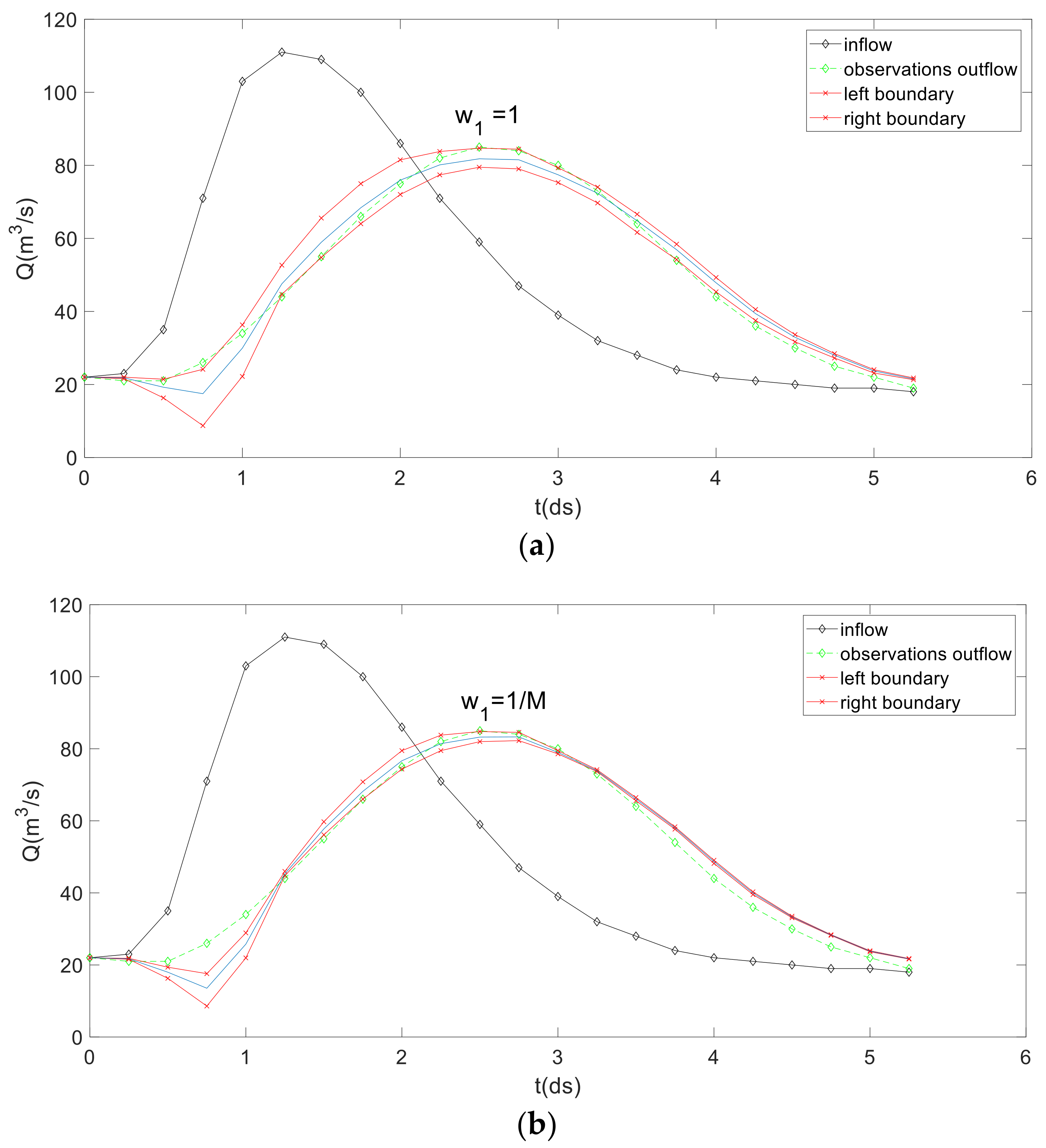
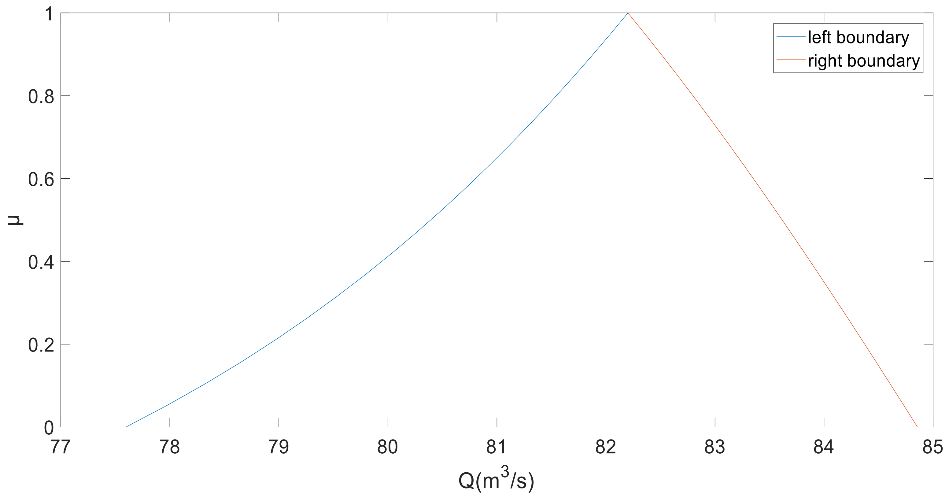
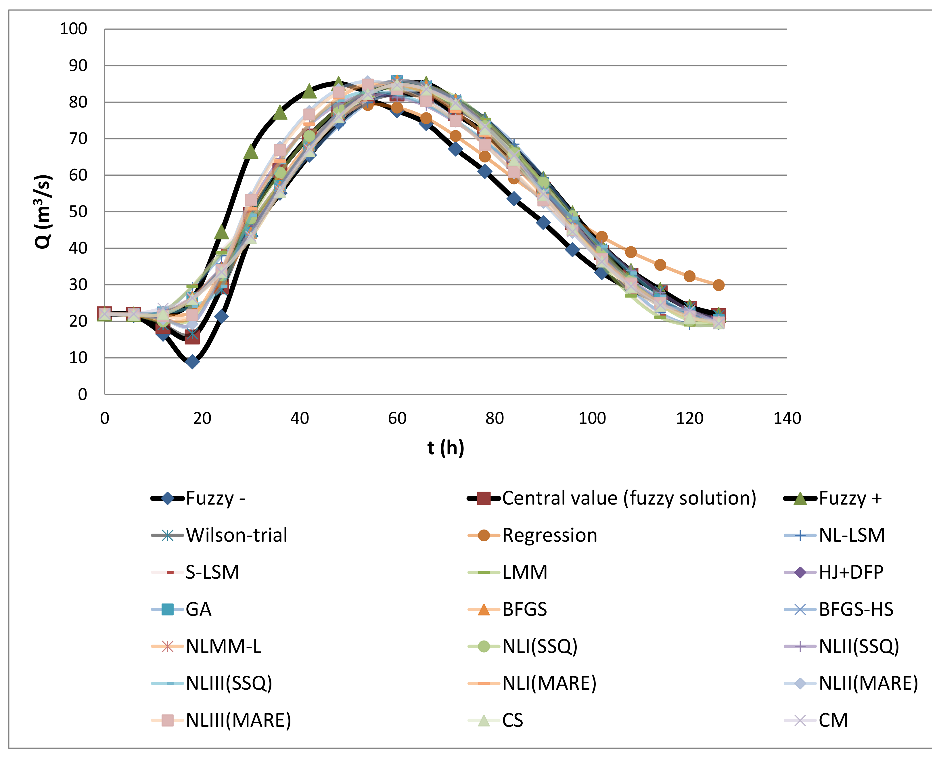
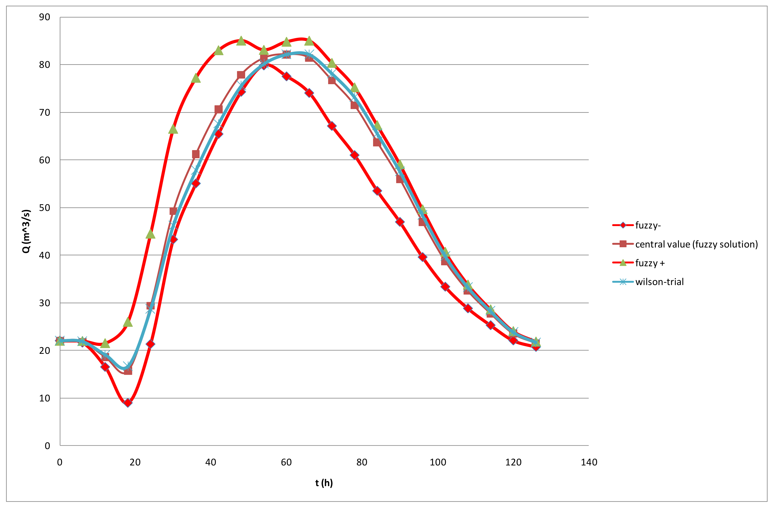
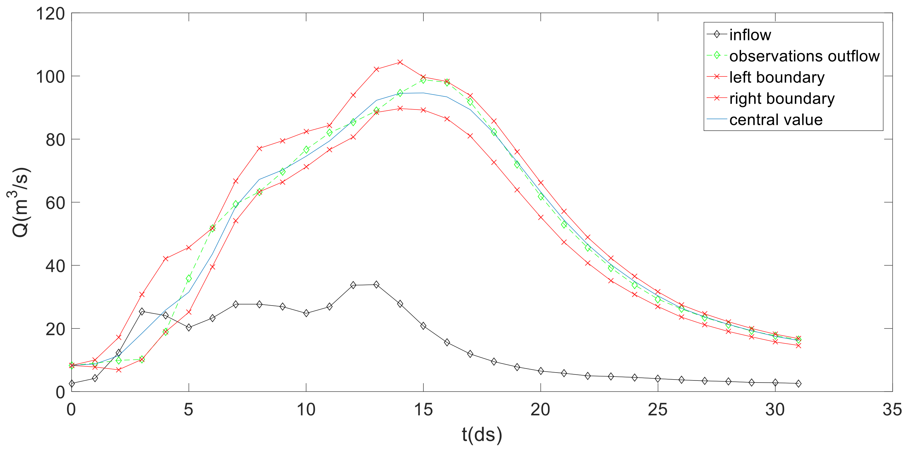
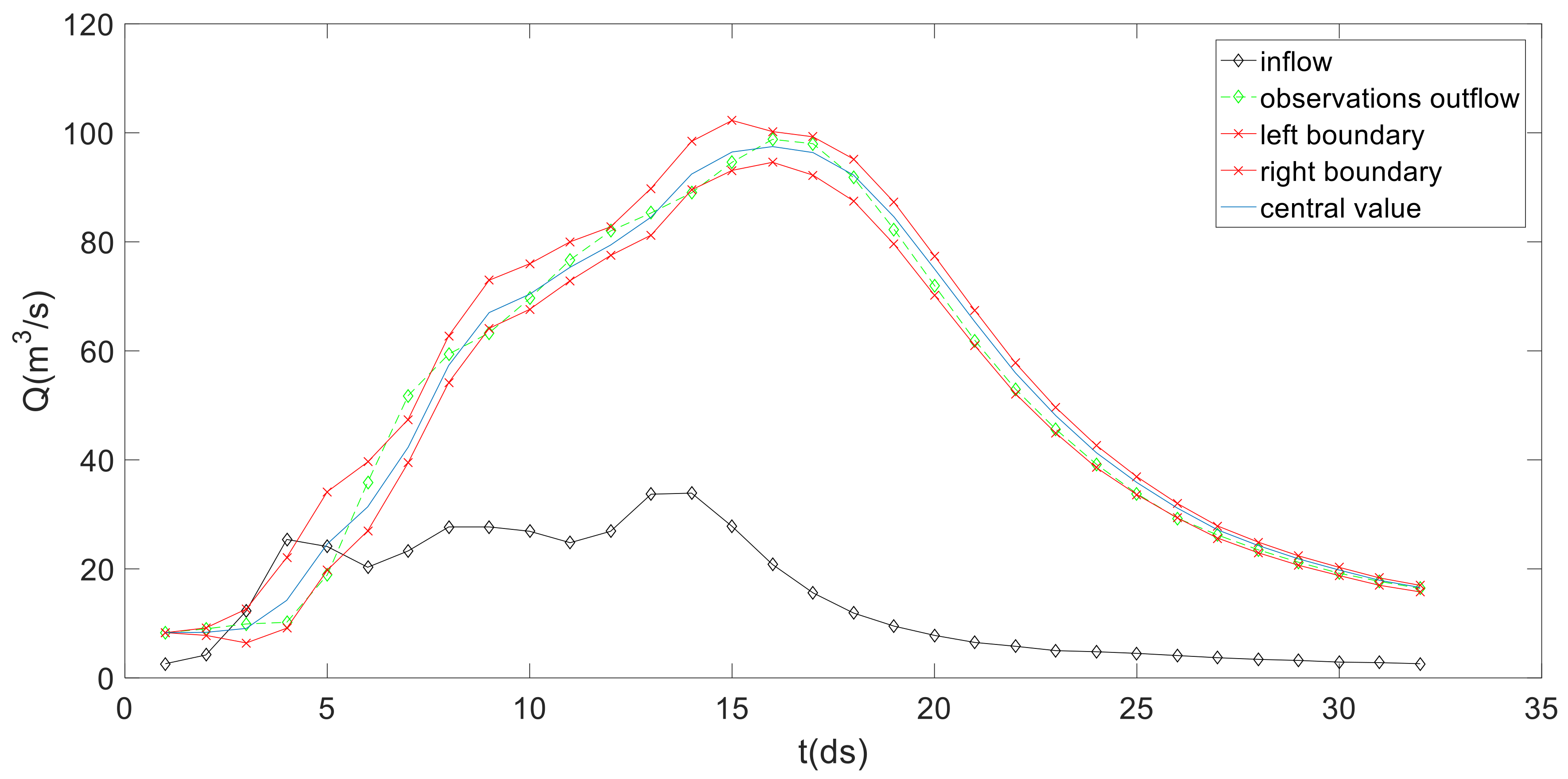
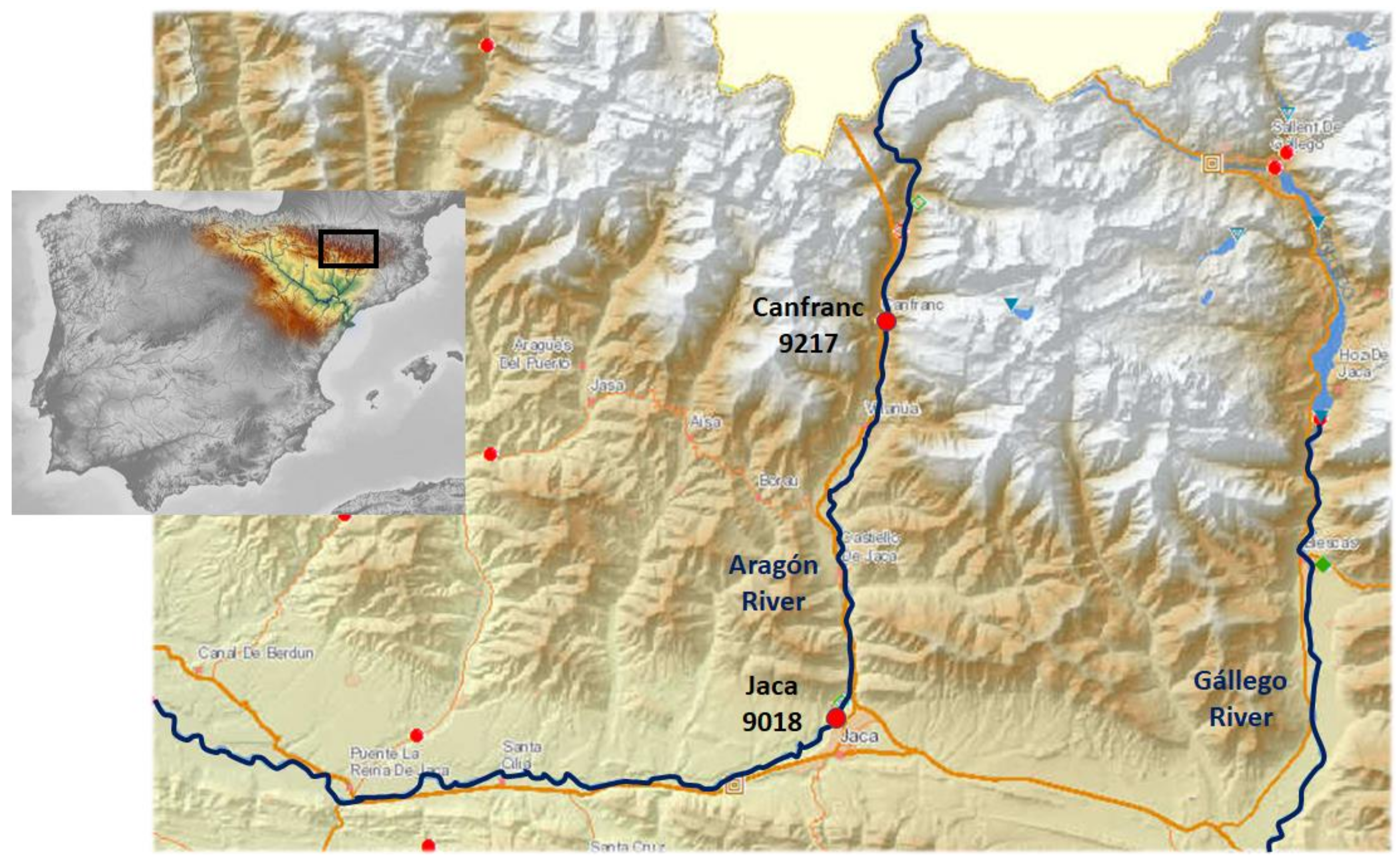
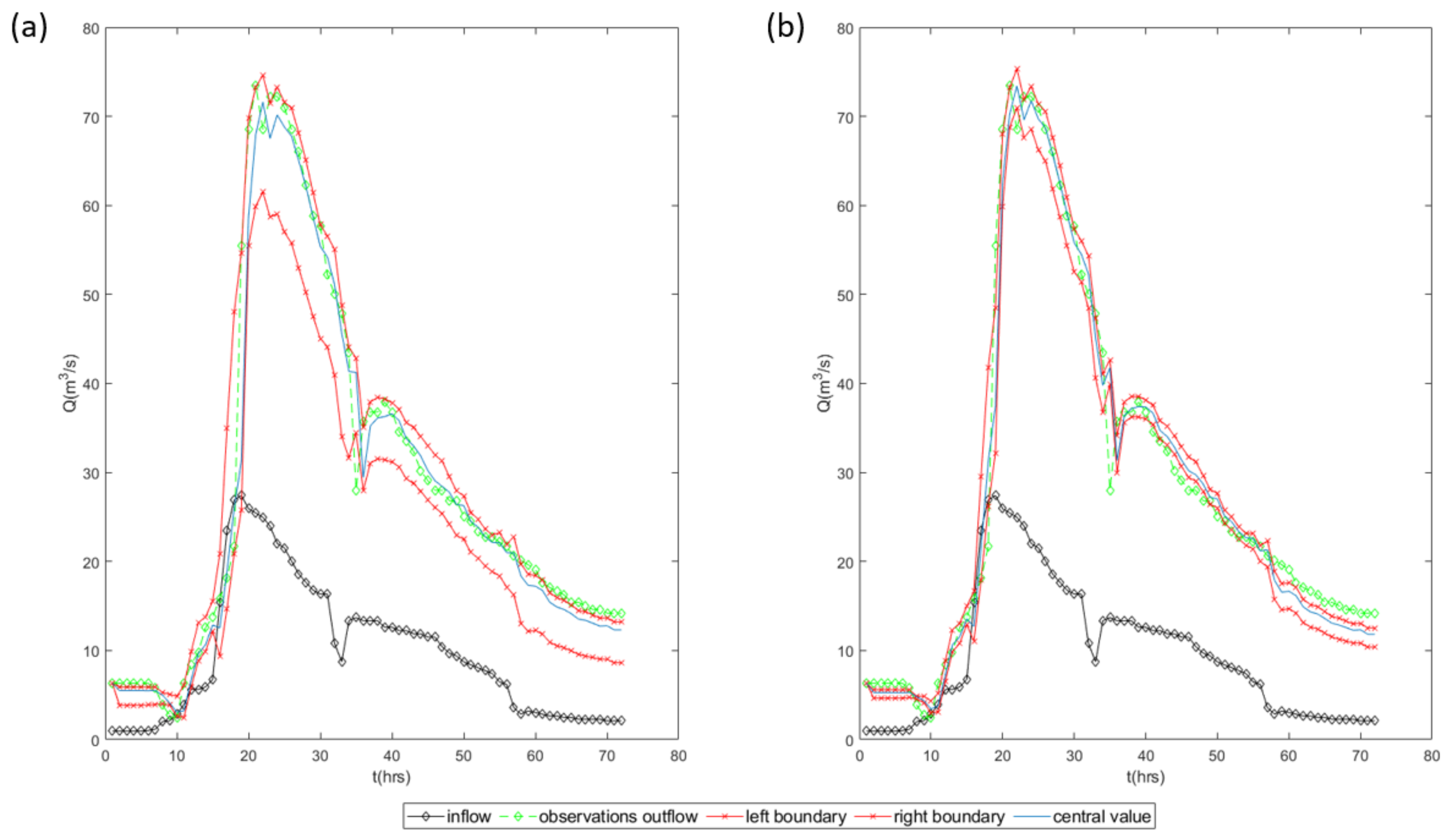
4.4. Validation with Real-Life Data

The validation case study is located in the Ebro River Basin (Spain, Figure 14). The gauge stations (automatic flow measures) belong to the SAIH network (Automatic Hydrologic Information System) managed by the Ebro Basin Water Authority. The reach under analysis is located in the Aragón River between stations 9271 (elevation 1040 m, basin area 101 km²) and 9018 (elevation 793 m, basin area 238 km²). The reach length is 18.09 km, and the mean slope of the reach is 1.365%. The method proposed in this study is validated with four hydrographs recently recorded in the reach. The time step of the original data is equal to 15 min. In order to reduce computational time and for stability reasons, the original data were resampled at Δt = 1 h time step. The selected hydrographs can be characterized as rather complex since they include important lateral flow, and their shapes are not smooth.

The performance of the method is tested by fitting the Muskingum parameters in one hydrograph (Hydrograph 1) and validating the prediction obtained with the fitted parameters for the three remaining hydrographs (Hydrographs 2, 3, and 4). The predictive capability of the method was tested for two values of parameter w₁: 1 and 0.1. The value of w₁: equal to one gives more weight on the inclusion of observations within the fuzzy band, while the value of w₁ equal to 0.1 gives more weight on the reduction of the uncertainty of the forecast. The results obtained for $w_1=1$ after 100 iterations are $\tilde{K}=\left(5.1605,3.5130\right)\mathrm{h},\tilde{x}=\left(0.1773,0.0495\right),\mathrm{and}\tilde{a}=\left(1.5160,0.4579\right)$. The results obtained for $w_1=0.1$ are $\tilde{K}=\left(3.8328,1.5637\right)\mathrm{h},\tilde{x}=\left(0.2273,0.0006\right),\mathrm{and}\tilde{a}=\left(1.8568,0.1930\right)$. The fuzzy bands obtained for the outflow hydrographs are presented in Figure 15. In both cases, the most relevant values of the outflow hydrograph (near the peak discharge) are included within the produced fuzzy band. The wider fuzzy band for w₁ = 1 includes a larger fraction of values, but the narrower fuzzy band for w₁ = 0.1 reduces the uncertainty of the forecast.

Afterwards, the fuzzy parameter values obtained for the two solutions were validated by applying them on three other real events, named Hydrograph 2, 3, and 4. The results are shown in Figure 16. For the fuzzy parameters obtained with hydrograph 1 and w₁ = 1, the stronger emphasis on the inclusion during the calibration process leads to results for other events where the observed outflow is almost included within the fuzzy band produced.

This aspect is quantified with the following modified measure E₁:

$${\overline{E}}_1=\underset{includingalldata}{\frac{1}{M}\left[{\displaystyle \sum _{j=1}^M{a}_{R_j}{\left(Q_j^{observed}-Q_j^{+}\right)}^2}+{\displaystyle \sum _{j=1}^M{a}_{L_j}{\left(Q_j^{-}-Q_j^{observed}\right)}^2}\right]},$$

The values of the modified measure obtained for Hydrographs 2, 3, and 4 are 0.6556, 0.3304, and 0.2526. These values are small, indicating a good coverage of the observations, although most of the observed discharges are below the central values of the fuzzy band.

For the fuzzy parameters obtained with Hydrograph 1 and w₁ = 0.1, the observed outflow is not included within the produced fuzzy band in most cases (Figure 16a). However, the shape of the observed outflow is similar to the produced fuzzy bands, suggesting that the deviation may be due to the different contribution of incremental flow in each event. The values of the modified measure are 6.8537, 10.8548, and 4.8134 (

Table 2. Modified measure E₁ (property of inclusion) and E₃ (uncertainty) by testing weights w₁ = 0.1 and w₁ = 1 and applied to Hydrographs 1 (training) and 2, 3, and 4 (validation).

	Training	Validation
	Hydrograph 1	Hydrograph 2	Hydrograph 3	Hydrograph 4
	w1 = 0.1
E1	3.8382	6.8537	10.8548	4.8134
E3	18.8438	24.9167	41.3546	20.9019
	w1 = 1
E1	0.7458	0.6556	1.1253	0.4815
E3	84.5021	79.5274	144.0766	75.1660

). As aforementioned, the property of inclusion (which is expressed by the modified measure E₁) is in conflict with the goal of low uncertainty, which is expressed by the measure E₃ (Table 2).

These fuzzy parameters showed a good skill to produce operational forecasts based only on inflow to the reach. The results were encouraging, particularly considering that incremental flow was important in comparison with the inflow to the reach. The parameter w₁ could be used to control whether the emphasis should be placed on inclusion of the observations within the fuzzy band or in narrowing the uncertainty of the predictions. It should be noted that important hydrograph’s characteristics were simulated with a high degree of accuracy, for example, the volume of the hydrograph, the peak flow, the lag time, and the duration of the hydrographs, among others.

In this validation exercise, the effectiveness of behavioral parameters was tested against an alternative parameter configuration proposed by Pedersen and Chipperfield [55], who suggested to simplify the approach by eliminating the use of the particle’s previous best-known position by setting c₁ = 0. The performance of this option was lower than that of the traditional values for behavioral parameters in the examined case. The small improvement in computation time was not found to be relevant because the large computation time is caused by the simulation (based on the extension principle) and not by the topology of the network and the corresponding update of the positions of the swarm. Therefore, the simplification of the topology of the swarm in this problem cannot win computational time and leads to poorer results.

A critical point of which these kind of studies should be aware is the number of data. For instance, the approach of the ANFIS system based on the Wilson, 1974 data [10] is not a safe choice since the ANFIS requires several variables. Furthermore, the use of sophisticated non-linear Muskingum models with either 10 [54] or significantly large [56] calibrated parameters, with only 18 sets of data available, have the risk of overtraining.

A disadvantage of the proposed methodology is the high computational time consumption required and secondly, the selection of the proper weight w₁, which differentiates the solution. However, (1) the production of a functional uncertainty (2) with parameters that make physical sense and (3) the inclusion of the observed data to a high degree, especially near the maximum value, will be the determinant criteria in the selection of the weight. For instance, in the case of the third example, a large quantity of w₁ leads to an unfunctional uncertainty as well as an irrational values for the parameter x.

An extension of the proposed methodology could be the application of a nonlinear form regarding the Muskingum model. However, two limitations must be taken into account. The first one is that a significant number of data is required for calibration, and the second is the difficulty in the incorporation of the fuzziness. Indeed, by using the linear Muskingum theory, an explicit relation exists to determine the outflow with respect to the parameters K and x (and α for lateral flow), while in the case of the nonlinear relation, a process with many steps is required. Hence, in the first case, the extension principle can be directly applied to determine the selected h-cuts.The more traditional optimization problems are gradient-based and local search algorithms, and hence the final optimum solutions, may depend on the consideration of the initial point. The evolutionary algorithms, such as genetic algorithm (GA) and swarm intelligence, has an advantage that overcomes this difficulty. Such global optimizers are in most cases simple, flexible, and efficient. However, it lacks in-depth understanding of how such algorithms may converge and how quickly they can converge to the global optimum, and hence, this point is a topic for further investigation [57]. The PSO method is selected because of its simplicity and since it has been applied in the examined problem of river routing with satisfactory results ([21,58,59]). Indeed, [60] suggested that their outcomes confirmed that the PSO algorithm estimated the parameters in a complex nonlinear Muskingum model with high accuracy along with a fast rate of convergence. In addition, in the examined case, which is a calibration problem, we can suppose a possible range of the parameters, and hence, a randomly created initial swarm can be easily constructed. The use of other heuristic algorithms is challenging especially in more complex simulation where a lateral flow exist, and the no linear Muskingum model may be adopted. For instance, the use of hybrid simulated annealing-PSO methods [61]) seem promising alternatives for further work. As it is written in [61], many algorithms introduce ideas that could be easily exported to other methods with varying degrees of compatibility. In [62], these hybrid models were proposed in the case of a water-based algorithm (e.g., [62]). For instance, by a similar way with the PSO, rain-fall optimization algorithm (RFO) has been applied as a new, naturally inspired algorithm based on behavior of raindrops with an effective approach [63].

The utility of the method might be extended in the cases of the rain-runoff models since some conceptual models use the well-known Muskingum method to express the quick flow development (instead of the unit hydrograph theory) and, with other parameters, the slow flow development [1].

5. Concluding Remarks

A general methodology to assess the parameter of the linear Muskingum model for river routing by considering parameters as fuzzy symmetrical triangular numbers is presented in this study. The expanded linear Muskingum storage method presented by O’Donnel (1985) [11] is used also in cases where a lateral flow occurs. Since the calibration model is an optimization of a case model, the PSO is used since it enables us to use a simulation process for each possible solution that composes the swarm. Hence, for each candidate solution, the extension principle of fuzzy sets and logic is activated in order to determine a fuzzy band of the outflow.

A fitness function is established that expresses the divergence of the produced fuzzy band to include all data. It takes into account the distance between the central values and the observed data, the total width of the fuzzy band and the distance between the maximum value of the outflow, and the right hand of the estimated outflow. A critical point is that the aim of divergence of the produced fuzzy band to include all data (property of inclusion) is in conflict with the aim of minimization of the total width of the produced fuzzy band. A weighted sum of the above goals composes the fitness function, whilst a functional width that contains most of the observed data is applied to select the weights of the fitness function.

Four case studies from the references are used to benchmark the proposed method, including smooth and non-smooth hydrographs with lateral flow and a double peak hydrograph. The last case study includes a complicated, real case study, and it is used for validation purposes. The proposed methodology improve results with the use of a fuzzy estimation with the aim of fuzzy parameters closer to nature; the new methodology increases the safety of the prediction; and furthermore, the produced fuzzy band can include, to a significant degree, the observed data and the output of the existent crisp methodologies even if they include a more complex formulation. Regarding the PSO model, results suggest that 100 iterations of a swarm with 50 members is sufficient to approach the final solution, while the candidates solutions converge to the total optimum.

References

1. Baymani-Nezhad, M.; Han, D. Hydrological modeling using Effective Rainfall routed by the Muskingum method (ERM). J. Hydroinformatics 2013, 15, 1437–1455. [Google Scholar] [CrossRef]
2. Niazkar, M.; Afzali, S.H. Streamline performance of Excel in stepwise implementation of numerical solutions. Comput. Appl. Eng. Educ. 2016, 24, 555–566. [Google Scholar] [CrossRef]
3. McCarthy, G.T. The Unit Hydrograph and Flood Routing; Conf. of North Atlantic Division, U.S. Army Corps of Engineers, Engineer Department at New London: New London, CT, USA, 24 June 1938. [Google Scholar]
4. Cunge, J.A. On the subject of a flood propagation computation method (Muskingum method). J. Hydraul. Res. 1969, 7, 205–230. [Google Scholar] [CrossRef]
5. Ponce, V.M.; Yevjevich, V. Muskingum-Cunge Method with Variable Parameters. J. Hydraul. Div. 1978, 104, 1663–1667. [Google Scholar] [CrossRef]
6. Ponce, V.; Lohani, A.; Scheyhing, C. Analytical verification of Muskingum-Cunge routing. J. Hydrol. 1996, 174, 235–241. [Google Scholar] [CrossRef]
7. Das, A. Parameter Estimation for Muskingum Models. J. Irrig. Drain. Eng. 2004, 130, 140–147. [Google Scholar] [CrossRef]
8. Akbari, G.H.; Barati, R. Comprehensive analysis of flooding in unmanaged catchments. Proc. Inst. Civil Eng. Water Manag. 2012, 165. [Google Scholar] [CrossRef]
9. Viessman, J.; Lewis, G.L. Introduction to Hydrology; Pearson Education, Inc.: Upper Saddle River, NJ, USA, 2011. [Google Scholar]
10. Wilson, E.M. Engineering Hydrology; Macmillan Education LTD: Hampshire, UK, 1974. [Google Scholar]
11. O’Donnel, T. A direct three-parameter Muskingum procedure incorporating lateral inflow. Hydrol. Sci. J. 1985, 30, 479–496. [Google Scholar] [CrossRef] [Green Version]
12. Spiliotis, M.; Sordo-Word, A.; Garrote, L. Estimation of the Muskingum Routing Coefficients Including Lateral inflow by using Fuzzy Linear Regression. In Proceedings of the 5th IAHR EUROPE CONGRESS, “New Challenges in Hydraulic Research and Engineering”, Trento, Italy, 12–14 June 2018; Armanini, A., Nucci, E., Eds.; The International Association for Hydro-Environment Engineering and Research: Beijing, China, 2018. [Google Scholar] [CrossRef]
13. Gill, M.A. Flood routing by the Muskingum method. J. Hydrol. 1978, 36, 353–363. [Google Scholar] [CrossRef]
14. Tung, Y.-K. River Flood Routing by Nonlinear Muskingum Method. J. Hydraul. Eng. 1985, 111, 1447–1460. [Google Scholar] [CrossRef] [Green Version]
15. Yoon, J.; Padmanabhan, G. Parameter Estimation of Linear and Nonlinear Muskingum Models. J. Water Resour. Plan. Manag. 1993, 119, 600–610. [Google Scholar] [CrossRef]
16. Geem, Z.W. Parameter Estimation for the Nonlinear Muskingum Model Using the BFGS Technique. J. Irrig. Drain. Eng. 2006, 132, 474–478. [Google Scholar] [CrossRef]
17. Geem, Z.W. Parameter Estimation of the Nonlinear Muskingum Model using Parameter-Setting-Free Harmony Search Algorithm. J. Hydraul. Res. 2011, 16, 684–688. [Google Scholar]
18. Karahan, H.; Gürarslan, G.; Geem, Z.W. A new nonlinear Muskingum flood routing model incorporating lateral flow. Eng. Optim. 2014, 47, 737–749. [Google Scholar] [CrossRef]
19. Mohan, S. Parameter Estimation of Nonlinear Muskingum Models Using Genetic Algorithm. J. Hydraul. Eng. 1997, 123, 137–142. [Google Scholar] [CrossRef]
20. Kim, J.H.; Geem, Z.W.; Kim, E.S. Parameter Estimation of the Nonlinear Muskingum Model Using Harmony Search. JAWRA J. Am. Water Resour. Assoc. 2001, 37, 1131–1138. [Google Scholar] [CrossRef]
21. Chu, H.-J.; Chang, L.-C. Applying Particle Swarm Optimization to Parameter Estimation of the Nonlinear Muskingum Model. J. Hydrol. Eng. 2009, 14, 1024–1027. [Google Scholar] [CrossRef]
22. Xu, D.-M.; Qiu, L.; Chen, S.-Y. Estimation of Nonlinear Muskingum Model Parameter Using Differential Evolution. J. Hydrol. Eng. 2012, 17, 348–353. [Google Scholar] [CrossRef]
23. Geem, Z.W.; Roper, W.E. Various continuous harmony search algorithms for web-based hydrologic parameter optimisation. Int. J. Math. Model. Numer. Optim. 2010, 1, 213–226. [Google Scholar] [CrossRef]
24. Niazkar, M.; Afzali, S.H. Assessment of Modified Honey Bee Mating Optimization for Parameter Estimation of Nonlinear Muskingum Models. J. Hydrol. Eng. 2015, 20, 04014055. [Google Scholar] [CrossRef]
25. Niazkar, M.; Afzali, S.-H. Application of New Hybrid Optimization Technique for Parameter Estimation of New Improved Version of Muskingum Model. Water Resour. Manag. 2016, 30, 4713–4730. [Google Scholar] [CrossRef]
26. Easa, S.M. Evaluation of nonlinear Muskingum model with continuous and discontinuous exponent parameters. KSCE J. Civ. Eng. 2015, 19, 2281–2290. [Google Scholar] [CrossRef]
27. Farzin, S.; Singh, V.P.; Karami, H.; Farahani, N.; Ehteram, M.; Kisi, O.; Allawi, M.F.; Mohd, N.S.; El-Shafie, A. Flood Routing in River Reaches Using a Three-Parameter Muskingum Model Coupled with an Improved Bat Algorithm. Water 2018, 10, 1130. [Google Scholar] [CrossRef] [Green Version]
28. Chu, H.-J. The Muskingum flood routing model using a neuro-fuzzy approach. KSCE J. Civ. Eng. 2009, 13, 371–376. [Google Scholar] [CrossRef]
29. Spiliotis, M.; Garrote, L. Estimation of the Muskingum routing coefficients by using fuzzy regression. Eur. Water 2017, 57, 133–140. [Google Scholar]
30. Tanaka, H. Fuzzy data analysis by possibilistic linear models. Fuzzy Sets Syst. 1987, 24, 363–375. [Google Scholar] [CrossRef]
31. Klir, G.; Yuan, B. Fuzzy Sets and Fuzzy Logic Theory and its Applications; Prentice Hall: New York, NY, USA, 1995. [Google Scholar]
32. Zimmermann, H.J. Fuzzy Set Theory and Its Applications; Springer Seience+Business Media: New York, NY, USA, 2001. [Google Scholar]
33. Buckley, J.; Eslami, E. Introduction to Fuzzy Logic and Fuzzy Sets (Advances in Soft Computing); Springer: Berlin/Heidelberg, Germany, 2002; Volume 13. [Google Scholar]
34. Buckley, J.; Eslami, E.; Feuring, T. Solving fuzzy equations. In Fuzzy Mathematics in Economics and Engineering; Buckley, J., Eslami, E., Feuring, T., Eds.; Springer: Berlin/Heidelberg, Germany, 2002; pp. 19–46. [Google Scholar]
35. Hanss, M. Applied Fuzzy Arithmetic, an Introduction with Engineering Applications; Springer: Berlin, Germany, 2005. [Google Scholar]
36. Spiliotis, M.; Angelidis, P.; Papadopoulos, B. A hybrid probabilistic bi-sector fuzzy regression based methodology for normal distributed hydrological variable. Evol. Syst. 2020, 11, 255–268. [Google Scholar] [CrossRef]
37. Tsakiris, G.; Spiliotis, M. Embankment dam break: Uncertainty of outflow based on fuzzy representation of breach formation param eters. J. Intell. Fuzzy Syst. 2014, 27, 2365–2378. [Google Scholar] [CrossRef]
38. Marsden, J.; Tromba, A. Vector Calculus, 5th ed.; W.H. Freeman and Company: New York, NY, USA, 2003. [Google Scholar]
39. Parsopoulos, K.E.; Vrahatis, M.N. Recent approaches to global optimization problems through particle swarm optimization. Nat. Comput. 2002, 1, 235–306. [Google Scholar] [CrossRef]
40. Spiliotis, M. A particle swarm optimization PSO heuristic for water distribution system analysis. Water Util. J. 2014, 8, 47–56. [Google Scholar]
41. Spiliotis, M.; Mediero, L.; Garrote, L. Optimization of Hedging Rules for Reservoir Operation During Droughts Based on Particle Swarm Optimization. Water Resour. Manag. 2016, 30, 5759–5778. [Google Scholar] [CrossRef]
42. Ostadrahimi, L.; Mariño, M.A.; Afshar, A. Multi-reservoir Operation Rules: Multi-swarm PSO-based Optimization Approach. Water Resour. Manag. 2011, 26, 407–427. [Google Scholar] [CrossRef]
43. Papadopoulos, Κ.; Papagianni, C.; Gkonis, P.; Venieris, I.; Kaklamani, D. Particle Swarm Optimization of Antenna Arrays with Efficiency Constraints. Prog. Electromagn. Res. M 2011, 17, 237–251. [Google Scholar] [CrossRef] [Green Version]
44. Spiliotis, M.; Garrote, L. Unit hydrograph identification based on fuzzy regression analysis. Evol. Syst. 2021, 1–22. [Google Scholar] [CrossRef]
45. Eberhart, R.C.; Kennedy, J. A new optimizer using particle swarm theory. In Proceedings of the Sixth Symposium on Micro Machine and Human Science, Nagoya, Japan, 4–6 October 1995; pp. 39–43. [Google Scholar] [CrossRef]
46. Poli, P.; Keenedy, J.; Blackwell, T. Particle swarm optimization. Swarm Intell. 2007, 1, 33–57. [Google Scholar] [CrossRef]
47. Shi, Y.; Eberhart, R. A modified particle swarm optimizer. In Proceedings of the 1998 IEEE International Conference on Evolutionary Computation Proceedings, Anchorage, AK, USA, 4–9 May 1998; pp. 69–73. [Google Scholar]
48. Clerc, M.; Kennedy, J. The particle swarm—Explosion, stability, and convergence in a multidimensional complex space. IEEE Trans. Evol. Comput. 2002, 6, 58–73. [Google Scholar] [CrossRef] [Green Version]
49. Salehizadeh, S.; Yadmellat, P.; Menhaj, M. Local Optima Avoidable Particle Swarm Optimization. In Proceedings of the IEEE Swarm Intelligence Symposium, Nashville, TN, USA, 30 March–2 April 2009; pp. 16–21. [Google Scholar]
50. Ishibuchi, H.; Tanaka, H.; Okada, H. An architecture of neural networks with interval weights and its application to fuzzy regression analysis. Fuzzy Sets Syst. 1993, 57, 27–39. [Google Scholar] [CrossRef]
51. Spiliotis, M.; Hrissanthou, V. Fuzzy and crisp regression analysis between sediment transport rates and stream discharge in the case of two basins in northeastern Greece. In Conventional and Fuzzy Regression: Theory and Engineering Applications; Hrissanthou, V., Spiliotis, M., Eds.; Nova Science Publishers: New York, NY, USA, 2018; pp. 1–46. [Google Scholar]
52. Tzimopoulos, C.; Papadopoulos, K.; Papadopoulos, B. Fuzzy Regression with Applications in Hydrology. Int. J. Eng. Innov. Technol. 2016, 5, 22. [Google Scholar]
53. Karahan, H.; Gürarslan, G.; Geem, Z.W. Parameter Estimation of the Nonlinear Muskingum Flood-Routing Model Using a Hybrid Harmony Search Algorithm. J. Hydrol. Eng. 2013, 18, 352–360. [Google Scholar] [CrossRef]
54. Karahan, H. Discussion of “Improved Nonlinear Muskingum Model with Variable Exponent Parameter” by Said M. Easa. J. Hydrol. Eng. 2014, 19, 07014007. [Google Scholar] [CrossRef]
55. Pedersen, M.; Chipperfield, A. Simplifying Particle Swarm Optimization. Appl. Soft Comput. 2010, 10, 618–628. [Google Scholar] [CrossRef]
56. Easa, S.M. Improved nonlinear Muskingum model with variable exponent parameter. J. Hydrol. Eng. 2013, 18, 1790–1794. [Google Scholar] [CrossRef]
57. Yang, X.-S. Nature-inspired optimization algorithms: Challenges and open problems. J. Comput. Sci. 2020, 46, 101104. [Google Scholar] [CrossRef] [Green Version]
58. Ouyang, A.; Tang, Z.; Li, K.; Sallam, A.; Sha, E. Estimating Parameters of Muskingum Model Using an Adaptive Hybrid pso Algorithm. Int. J. Pattern Recognit. Artif. Intell. 2014, 28, 1459003. [Google Scholar] [CrossRef]
59. Norouzi, H.; Bazargan, J. Flood routing by linear Muskingum method using two basic floods data using particle swarm optimization (PSO) algorithm. Water Supply 2020, 20, 1897–1908. [Google Scholar] [CrossRef]
60. Moghaddam, A.; Behmanesh, J.; Farsijani, A. Parameters Estimation for the New Four-Parameter Nonlinear Muskingum Model Using the Particle Swarm Optimization. Water Resour. Manag. 2016, 30, 2143–2160. [Google Scholar] [CrossRef]
61. Sudibyo, S.; Murat, M.N.; Aziz, N. Simulated annealing-Particle Swarm Optimization (SA-PSO): Particle distribution study and application in Neural Wiener-based NMPC. In Proceedings of the 2015 10th Asian Control Conference (ASCC), Kota Kinabalu, Malaysia, 31 May–3 June 2015; pp. 1–6. [Google Scholar]
62. Rubio, F.; Rodríguez, I. Water-Based Metaheuristics: How Water Dynamics Can Help Us to Solve NP-Hard Problems. Complexity 2019, 2019, 1–13. [Google Scholar] [CrossRef]
63. Clark, D. (Ed.) Kaboli, HRA Rain-Fall Inspired Optimization Algorithm For Optimal Load Dispatch In Power System. In Robust and Constrained Optimization: Methods and Applications; Nova Science Publishers: New York, NY, USA, 2020. [Google Scholar]
Figure 1. Representation of the membership function for a fuzzy number.
Sustainability 13 07152 g001
Figure 2. Fuzzy triangular symmetrical number.
Sustainability 13 07152 g002
Figure 3. Simulation of the Wilson (1974) [10] example based on the proposed fuzzy method for w1 = M2 in the case of the Wilson (1974) data.
Sustainability 13 07152 g003
Figure 4. Simulation of the Wilson (1974) [10] example based on the proposed fuzzy method for (a) w1 = 1 and (b) w1 = 1/M in the case of the Wilson (1974) data.
Sustainability 13 07152 g004
Figure 5. Simulation of the Wilson (1974) [10] example based on the proposed fuzzy method for w1 = M2 in case of the Wilson (1974) data. The blue circles indicate the swarm of the possible solution and the diamond the global optimum solution for each generation.
Sustainability 13 07152 g005
Figure 6. Produced outflow when the maximum outflow occurs in the real data in the case of the Wilson (1974) data for w1 = Μ2.
Sustainability 13 07152 g006
Figure 7. Other crisp simulations, the observed data, and the produced fuzzy band in case of the Wilson (1974) [10] data.
Sustainability 13 07152 g007
Figure 8. The graphical solution and the produced fuzzy band in the case of the Wilson (1974) data.
Sustainability 13 07152 g008
Figure 9. Simulation of the [9] example based on the proposed fuzzy method for w1 = M2. The blue line means the central values.
Sustainability 13 07152 g009
Figure 10. Simulation of the [9] example based on the proposed fuzzy method for w1 = 1. The blue line means the central values.
Sustainability 13 07152 g010
Figure 11. Other crisp simulations, the observed data ,and the produced fuzzy band in case of the [9] data for (a) w1 = M2 (b) w1 = 1.
Sustainability 13 07152 g011aSustainability 13 07152 g011b
Figure 12. The observed data and the produced fuzzy band in the case of the River Wyre, 20–21 October 1982 data for w1 = M2.
Sustainability 13 07152 g012
Figure 13. The observed data and the produced fuzzy band in the case of the River Wyre, 20–21 October 1982 data for w1 = 1.
Sustainability 13 07152 g013
Figure 14. Case study in Aragón River, Ebro Basin, Spain. The studied reach starts at Canfranc gauge station (red dot, Id 9217) and ends at Jaca gauge station (red dot, Id 9018).
Sustainability 13 07152 g014
Figure 15. Inflow and outflow hydrographs (data corresponding to Hydrograph 1) and the predicted fuzzy band of the Ebro River based on the proposed method for (a) w1 = 1 and (b) w1 = 0.1.
Sustainability 13 07152 g015
Figure 16. Validation of the achieved solution based on three real available hydrographs for (a) w1 = 0.1 and (b) w1 = 1. Left column corresponds to Hydrograph 2, central column to Hydrograph 3, and right column to Hydrograph 4.
Sustainability 13 07152 g016