
Evaluating Irrigation Performance and Water Productivity Using EEFlux ET and NDVI


Abstract
:1. Introduction
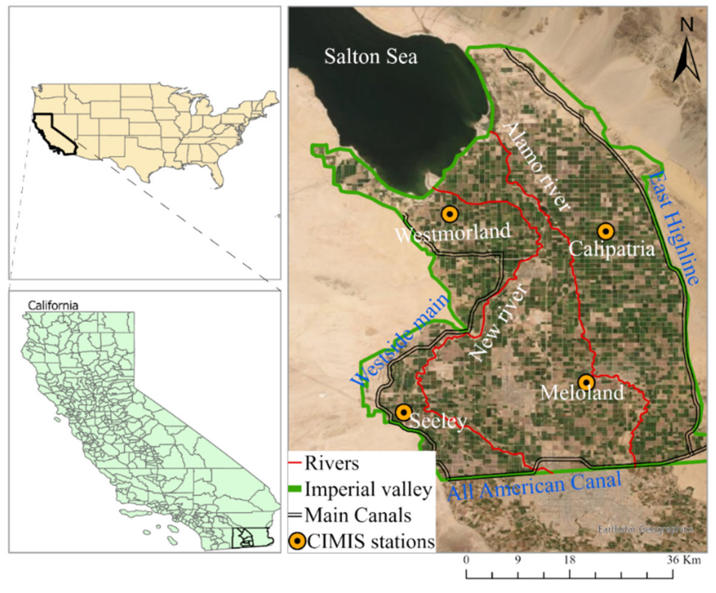
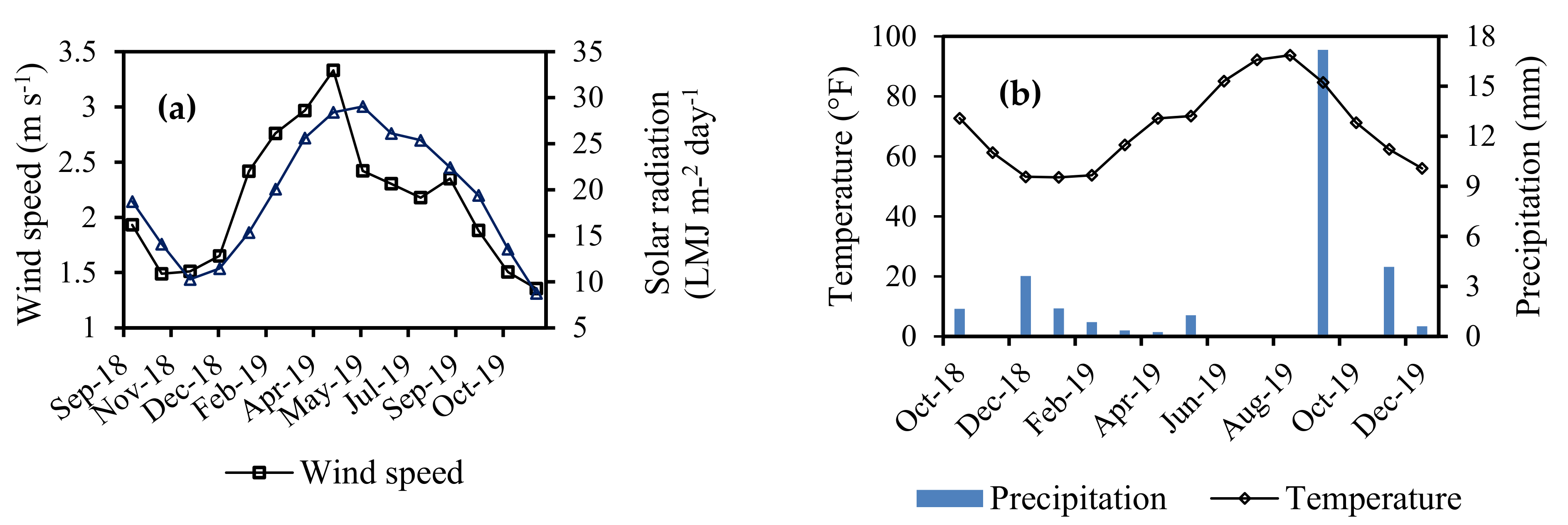
2. Study Area
3. Materials and Methods
3.1. Datasets
3.1.1. Google EEFlux Datasets
3.1.2. Satellite Images for NDVI Mapping
3.1.3. Reference Evapotranspiration
3.1.4. Data for the Crop Mapping and Validation
3.1.5. Other Datasets
3.2. Image Preprocessing
3.3. Crop Classification
3.4. Mapping the Seasonal ET
3.5. NDVI and Yield Mapping
3.6. Validation of ETa and Yield
3.7. Computation of the Performance Indicators
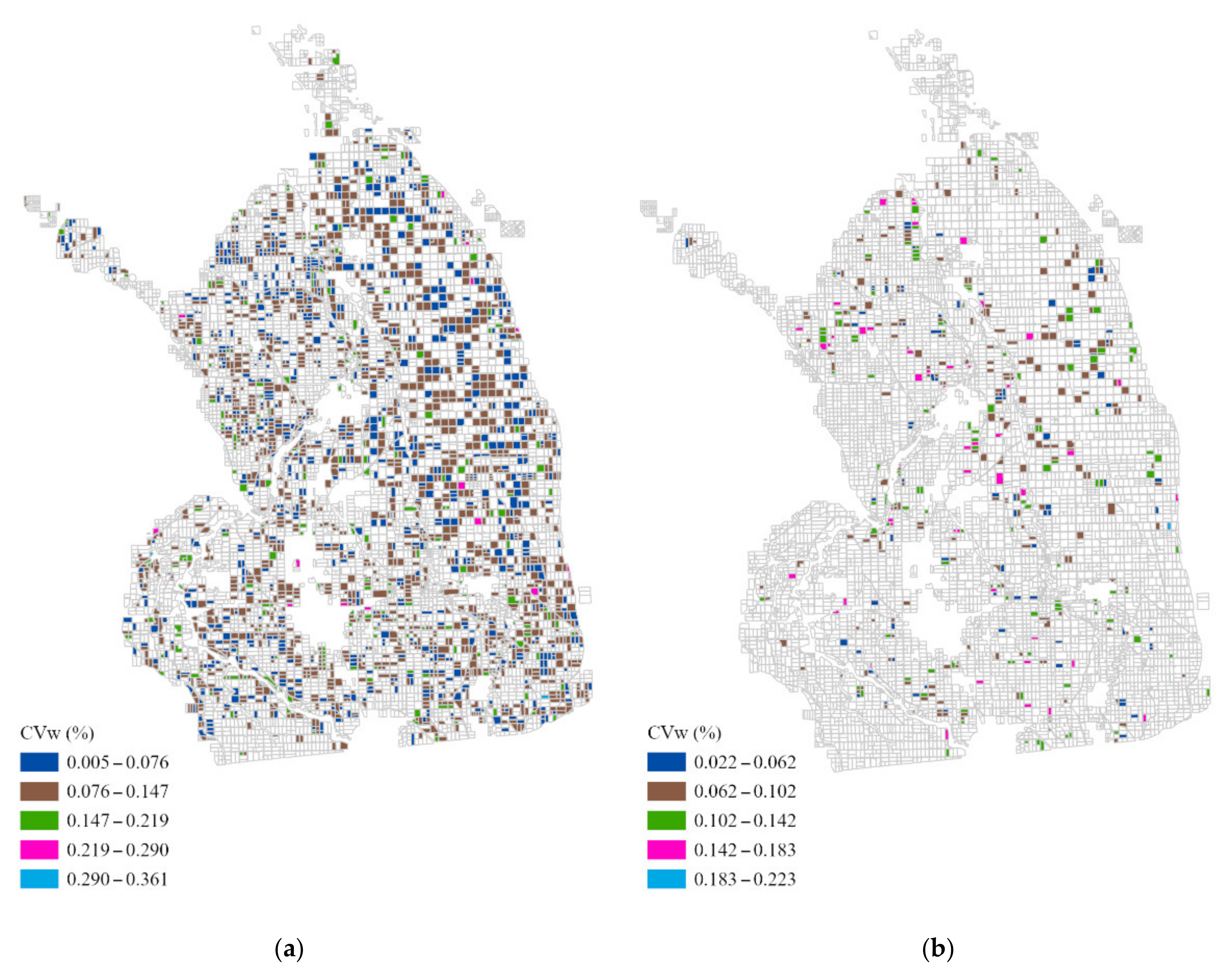
3.7.1. Water Consumption Uniformity (WCU)
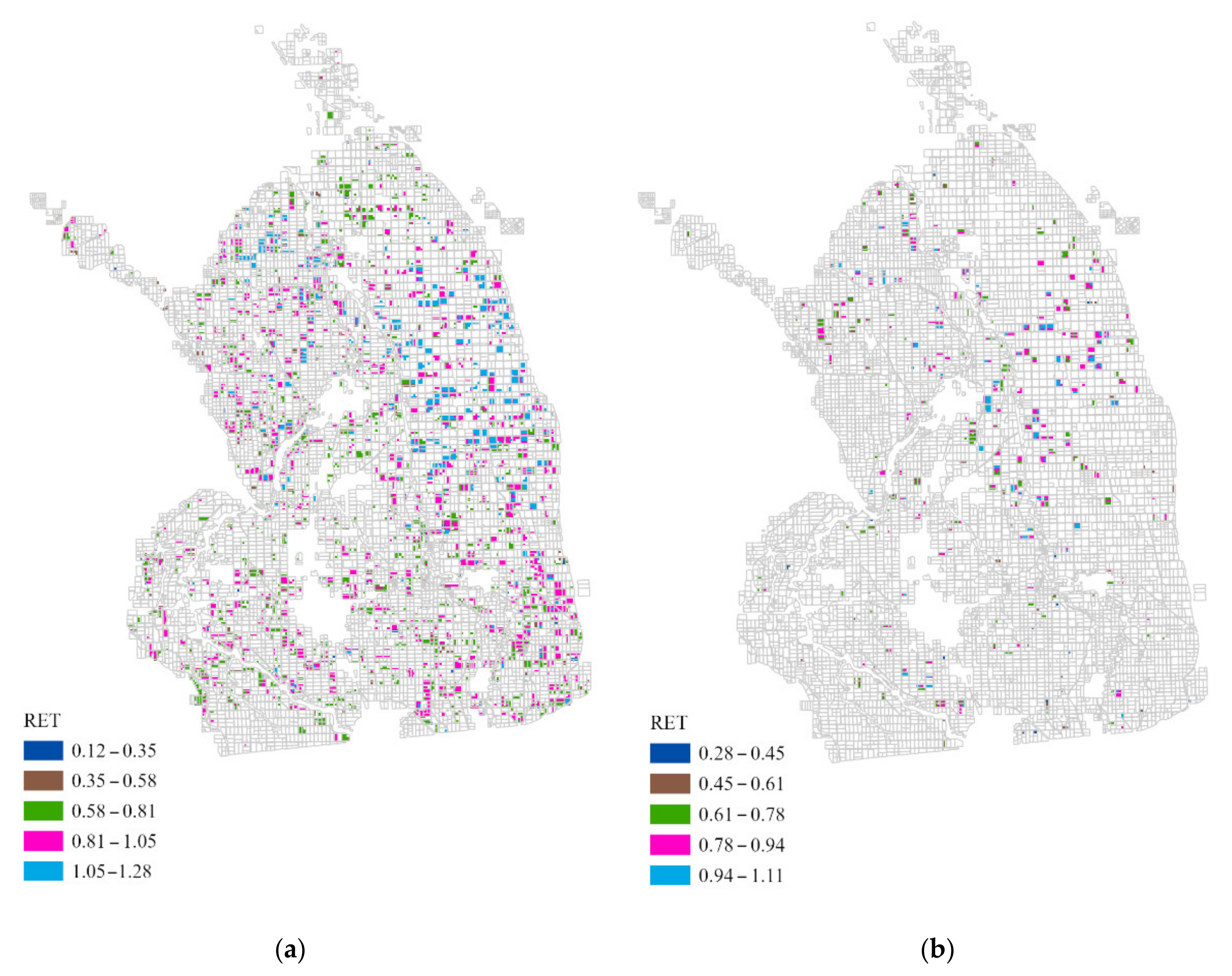
3.7.2. Relative Evapotranspiration (RET)
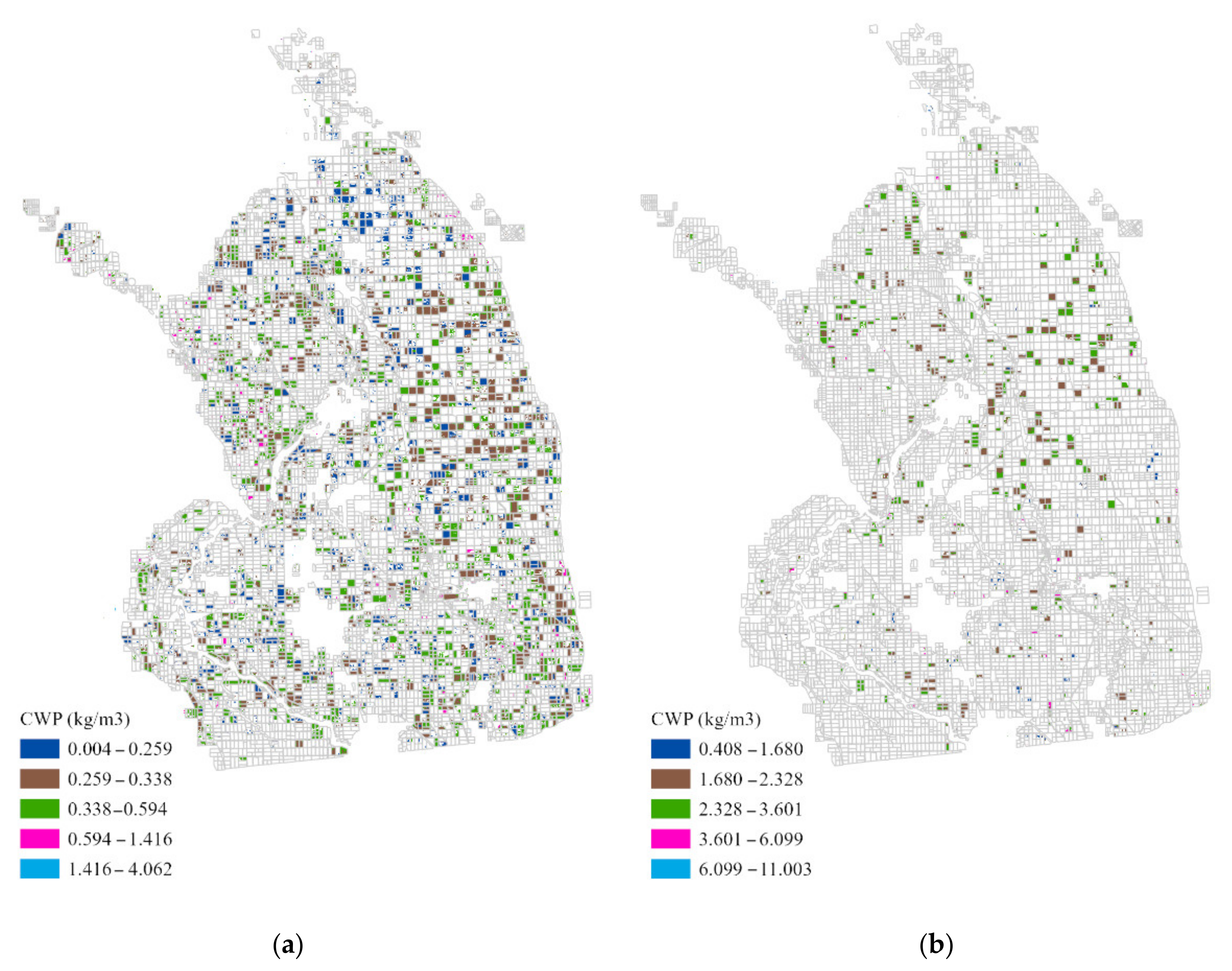
3.7.3. CWP
4. Results
4.1. Crop Classification
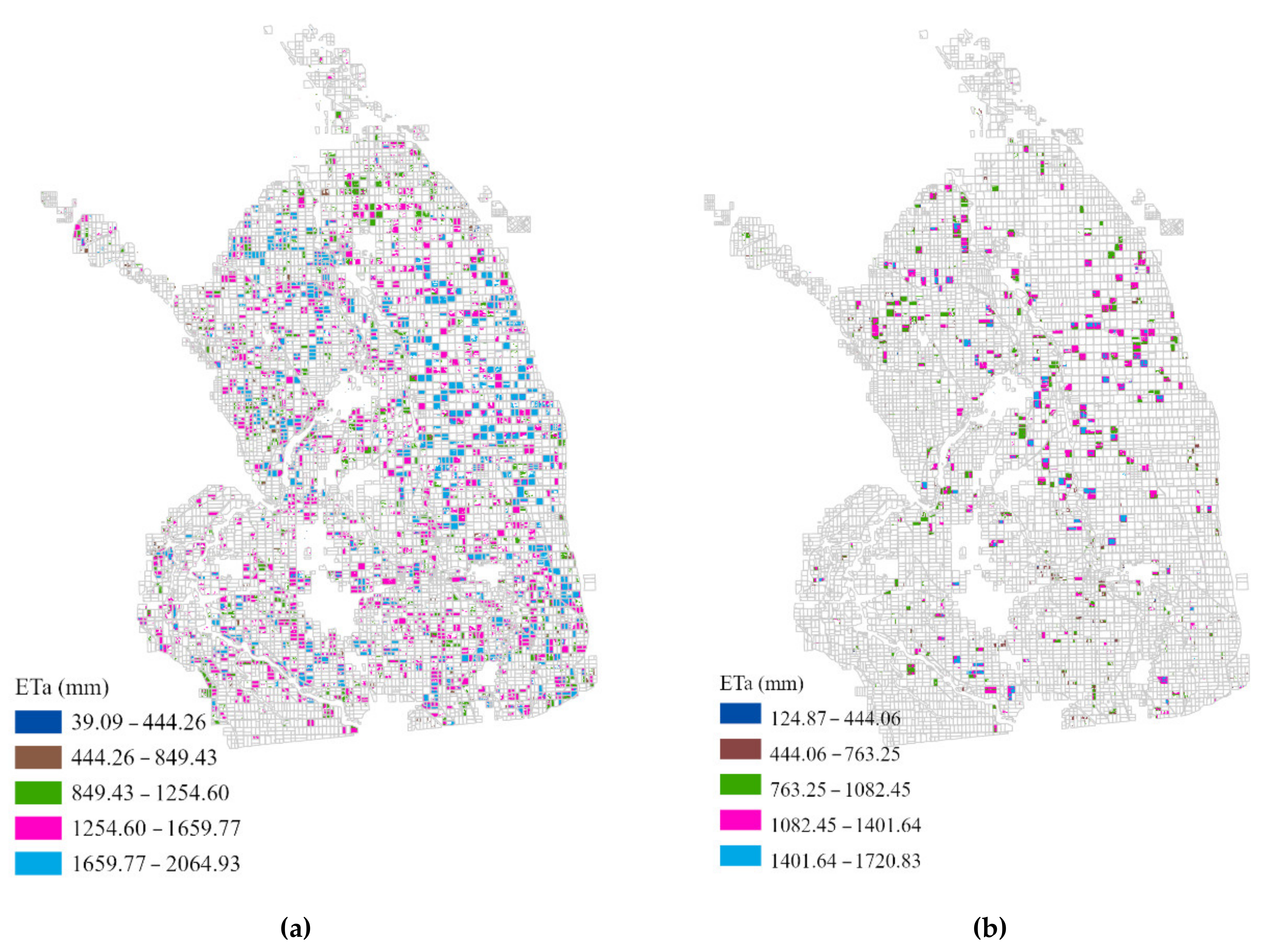
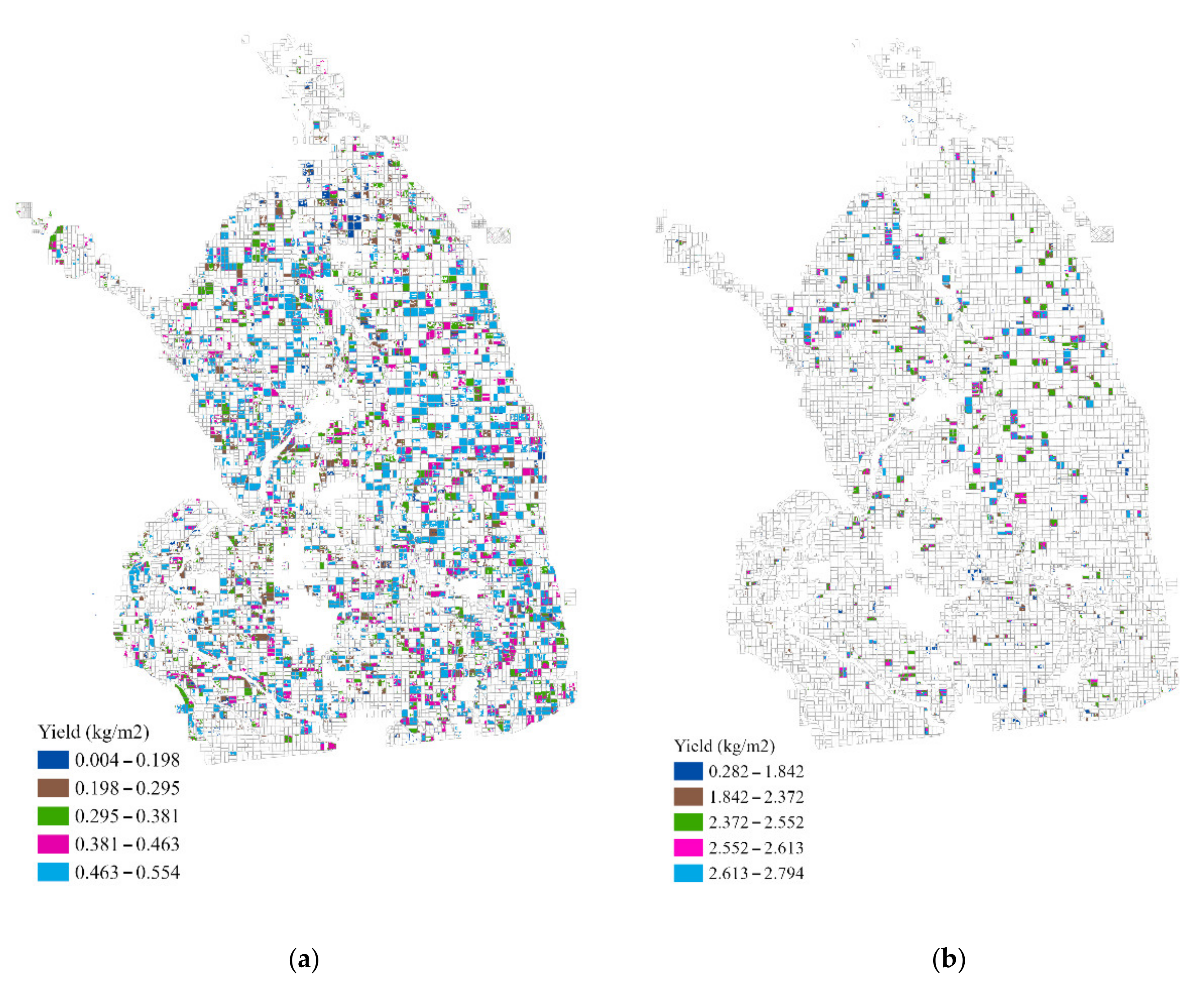
4.2. Spatial Distribution of ET and Yield
4.3. ET Validation
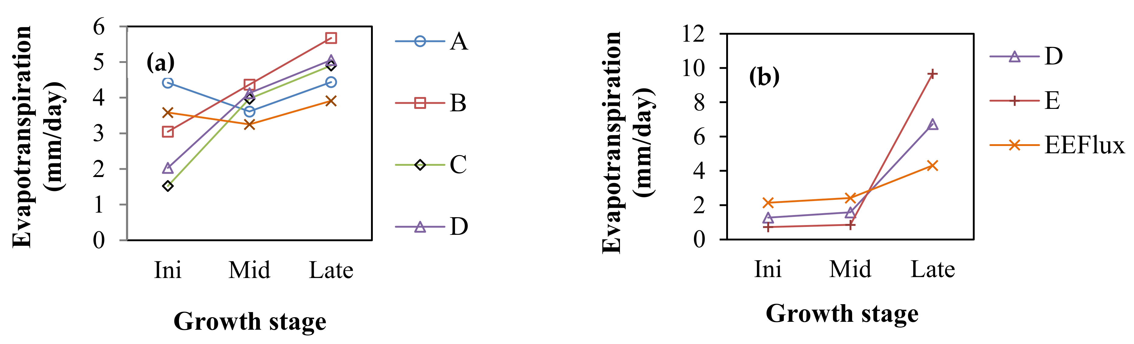
4.3.1. Comparison with the ET from the Literature
4.3.2. Comparison with the FAO-56-Computed ETc
4.4. Performance Indicators
4.4.1. WCU
4.4.2. RET
4.4.3. CWP
4.5. Analysis on the Scope of Water Conservation
5. Discussions
6. Conclusions
Author Contributions
Funding
Institutional Review Board Statement
Informed Consent Statement
Data Availability Statement
Conflicts of Interest
References
- González-Dugo, M.P.; Mateos, L. Spectral vegetation indices for benchmarking water productivity of irrigated cotton and sugarbeet crops. Agric. Water Manag. 2008, 95, 48–58. [Google Scholar] [CrossRef]
- Taghvaeian, S.; Neale, C.M.; Osterberg, J.C.; Sritharan, S.I.; Watts, D.R. Remote sensing and GIS techniques for assessing irrigation performance: Case study in Southern California. J. Irrig. Drain. Eng. 2018, 144, 05018002. [Google Scholar] [CrossRef]
- Dawadi, S.; Ahmad, S. Changing climatic conditions in the Colorado River Basin: Implications for water resources management. J. Hydrol. 2012, 430, 127–141. [Google Scholar] [CrossRef]
- Kalra, A.; Sagarika, S.; Pathak, P.; Ahmad, S. Hydro-climatological changes in the Colorado River Basin over a century. Hydrol. Sci. J. 2017. [Google Scholar] [CrossRef]
- Rahaman, M.M.; Thakur, B.; Kalra, A.; Ahmad, S. Modeling of GRACE-Derived Groundwater Information in the Colorado River Basin. Hydrology 2019, 6, 19. [Google Scholar] [CrossRef] [Green Version]
- Tamaddun, K.; Kalra, A.; Kumar, S.; Ahmad, S. CMIP5 Models’ Ability to Capture Observed Trends under the Influence of Shifts and Persistence: An In-depth Study on the Colorado River Basin. J. Appl. Meteorol. Climatol. 2019. [Google Scholar] [CrossRef]
- Bali, K.M.; Grismer, M.E.; Tod, I.C. Reduced-runoff irrigation of alfalfa in Imperial Valley, California. J. Irrig. Drain. Eng. 2001, 127, 123–130. [Google Scholar] [CrossRef]
- Sagarika, S.; Kalra, A.; Ahmad, S. Evaluating the effect of persistence on long-term trends and analyzing step changes in streamflows of the continental United States. J. Hydrol. 2014, 517, 36–53. [Google Scholar] [CrossRef]
- Ghumman, A.R.; Ahmad, S.; Khan, R.A.; Hashmi, H.N. Comparative Evaluation of Implementing Participatory Irrigation Management in Punjab Pakistan. Irrig. Drain. 2014, 63, 315–327. [Google Scholar] [CrossRef]
- Dawadi, S.; Ahmad, S. Evaluating the Impact of Demand-Side Management on Water Resources under Changing Climatic Conditions and Increasing Population. J. Environ. Manag. 2013, 114, 261–275. [Google Scholar] [CrossRef]
- Saher, R.; Stephen, H.; Ahmad, S. Understanding the summertime warming in canyon and non-canyon surfaces. Urban Clim. 2021. [Google Scholar] [CrossRef]
- Bukhary, S.; Batista, J.; Ahmad, S. Analyzing Land and Water Requirements for Solar Deployment in the Southwestern United States. Renew. Sustain. Energy Rev. 2018, 82, 3288–3305. [Google Scholar] [CrossRef]
- Qaiser, K.; Ahmad, S.; Johnson, W.; Batista, J.R. Evaluating the impact of water conservation on fate of outdoor water use: A study in an arid region. J. Environ. Manag. 2011, 92, 2061–2068. [Google Scholar] [CrossRef]
- Qaiser, K.; Ahmad, S.; Johnson, W.; Batista, J.R. Evaluating Water Conservation and Reuse Policies using a Dynamic Water Balance Model. Environ. Manag. 2013, 51, 449–458. [Google Scholar] [CrossRef] [PubMed]
- Ghumman, A.R.; Iqbal, M.; Ahmad, S.; Hashmi, H.N. Experimental and Numerical Investigations for Optimal Emitter Spacing in Drip Irrigation. Irrig. Drain. 2018, 67, 724–737. [Google Scholar] [CrossRef]
- Tamaddun, K.; Kalra, A.; Ahmad, S. Potential of rooftop rainwater harvesting to meet outdoor water demand in arid regions. J. Arid Land. 2018, 10, 68–83. [Google Scholar] [CrossRef] [Green Version]
- Ahmad, M.U.D.; Turral, H.; Nazeer, A. Diagnosing irrigation performance and water productivity through satellite remote sensing and secondary data in a large irrigation system of Pakistan. Agric. Water Manag. 2009, 96, 551–564. [Google Scholar] [CrossRef]
- Bastiaanssen, W.G.; Bos, M.G. Irrigation performance indicators based on remotely sensed data: A review of literature. Irrig. Drain. Syst. 1999, 13, 291–311. [Google Scholar] [CrossRef]
- Murray-Rust, H.; Snellen, W.B. Irrigation System Performance Assessment and Diagnosis; IWMI: Anand, India, 1993. [Google Scholar]
- Menenti, M.; Visser, T.; Morabito, J.A.; Drovandi, A. Appraisal of Irrigation Performance with Satellite Data and Georeferenced Information: The Rio Tunuyan Irrigation Scheme; Institute of Irrigation Studies, Southampton University: Southampton, UK, 1989. [Google Scholar]
- Moran, M.S. Irrigation management in Arizona using satellites and airplanes. Irrig. Sci. 1994, 15, 35–44. [Google Scholar] [CrossRef]
- Bastiaanssen, W.G.; Van der Wal, T.; Visser, T.N.M. Diagnosis of regional evaporation by remote sensing to support irrigation performance assessment. Irrig. Drain. Syst. 1996, 10, 1–23. [Google Scholar] [CrossRef]
- Roerink, G.J.; Bastiaanssen, W.G.; Chambouleyron, J.; Menenti, M. Relating crop water consumption to irrigation water supply by remote sensing. Water Resour. Manag. 1997, 11, 445–465. [Google Scholar] [CrossRef]
- Alexandridis, T.; Asif, S.; Ali, S. Water Performance Indicators Using Satellite Imagery for the Fordwah Eastern Sadiqia (South) Irrigation and Drainage Project; No. H024895; International Water Management Institute: Colombo, Sri Lanka, 1999. [Google Scholar]
- Bastiaanssen, W.G.M.; Thiruvengadachari, S.; Sakthivadivel, R.; Molden, D.J. Satellite remote sensing for estimating producitivities of land and water. Int. J. Water Resour. Dev. 1999, 15, 181–186. [Google Scholar] [CrossRef]
- Thiruvengadachari, S.; Sakthivadivel, R. Satellite Remote Sensing Techniques to Aid Irrigation System Performance Assessment: A Case study in India; Research Report 09; International Water Management Institute: Colombo, Sri Lanka, 1997; p. 31. [Google Scholar]
- Ambast, S.K.; Singh, O.P.; Tyagi, N.K.; Menenti, M.; Roerink, G.J.; Bastiaanssen, W.G.M. Appraisal of irrigation system performance in saline irrigated command using SRS and GIS. In Operational remote sensing for sustainable development; Balkema: Rotterdam, The Netherlands, 1999; pp. 457–461. [Google Scholar]
- Karatas, B.S.; Akkuzu, E.; Unal, H.B.; Asik, S.; Avci, M. Using satellite remote sensing to assess irrigation performance in Water User Associations in the Lower Gediz Basin, Turkey. Agric. Water Manag. 2009, 96, 982–990. [Google Scholar] [CrossRef]
- Kharrou, M.H.; Le Page, M.; Chehbouni, A.; Simonneaux, V.; Er-Raki, S.; Jarlan, L.; Chehbouni, G. Assessment of equity and adequacy of water delivery in irrigation systems using remote sensing-based indicators in semi-arid region, Morocco. Water Resour. Manag. 2013, 27, 4697–4714. [Google Scholar] [CrossRef]
- Geerts, S.; Raes, D. Deficit irrigation as an on-farm strategy to maximize crop water productivity in dry areas. Agric. Water Mana. 2009, 96, 1275–1284. [Google Scholar] [CrossRef] [Green Version]
- Cai, X.L.; Sharma, B.R. Integrating remote sensing, census, and weather data for an assessment of rice yield, water consumption and water productivity in the Indo-Gangetic River basin. Agric. Water Manag. 2010, 97, 309–316. [Google Scholar] [CrossRef]
- Immerzeel, W.W.; Gaur, A.; Zwart, S.J. Integrating remote sensing and a process-based hydrological model to evaluate water use and productivity in a south Indian catchment. Agric. Water Manag. 2008, 95, 11–24. [Google Scholar] [CrossRef]
- Yan, N.; Wu, B. Integrated spatial–temporal analysis of crop water productivity of winter wheat in Hai Basin. Agric. Water Manag. 2014, 133, 24–33. [Google Scholar] [CrossRef]
- Zwart, S.J.; Bastiaanssen, W.G. SEBAL for detecting spatial variation of water productivity and scope for improvement in eight irrigated wheat systems. Agric. Water Manag. 2007, 89, 287–296. [Google Scholar] [CrossRef]
- Ahmed, B.M.; Tanakamaru, H.; Tada, A. Application of remote sensing for estimating crop water requirements, yield, and water productivity of wheat in the Gezira Scheme. Int. J. Remote Sens. 2010, 31, 4281–4294. [Google Scholar] [CrossRef]
- Gorantiwar, S.D.; Smout, I.K. Performance assessment of irrigation water management of heterogeneous irrigation schemes: 1. A framework for evaluation. Irrig. Drain. Syst. 2005, 19, 1–36. [Google Scholar] [CrossRef] [Green Version]
- Usman, M.; Liedl, R.; Shahid, M.A. Managing irrigation water by yield and water productivity assessment of a rice-wheat system using remote sensing. J. Irrig. Drain. Eng. 2014, 140, 04014022. [Google Scholar] [CrossRef]
- Saher, R.; Stephen, H.; Ahmad, S. Urban evapotranspiration of Green Spaces in Arid Regions through Two Established Approaches: A Review of Key Drivers, Advancements, Limitations, and Potential Opportunities. Urban Water J. 2020. [Google Scholar] [CrossRef]
- Zhang, K.; Kimball, J.S.; Running, S.W. A review of remote sensing based actual evapotranspiration estimation. Wiley Interdiscip. Rev. Water 2016, 3, 834–853. [Google Scholar] [CrossRef]
- Kustas, W.P.; Norman, J.M. Use of remote sensing for evapotranspiration monitoring over land surfaces. Hydrol. Sci. J. 1996, 41, 495–516. [Google Scholar] [CrossRef]
- Reyes-González, A.; Kjaersgaard, J.; Trooien, T.; Hay, C.; Ahiablame, L. Estimation of crop evapotranspiration using satellite remote sensing-based vegetation index. Adv. Meteorol. 2018, 4525021. [Google Scholar] [CrossRef]
- Er-Raki, S.; Chehbouni, A.; Duchemin, B. Combining satellite remote sensing data with the FAO-56 dual approach for water use mapping in irrigated wheat fields of a semi-arid region. Remote Sens. 2010, 2, 375–387. [Google Scholar] [CrossRef] [Green Version]
- Bastiaanssen, W.G.; Menenti, M.; Feddes, R.A.; Holtslag, A.A.M. A remote sensing surface energy balance algorithm for land (SEBAL). 1. Formulation. J. Hydrol. 1998, 212, 198–212. [Google Scholar] [CrossRef]
- Allen, R.G.; Tasumi, M.; Trezza, R. Satellite-based energy balance for mapping evapotranspiration with internalized calibration (METRIC)—Model. J. Irrig. Drain. Eng. 2007, 133, 380–394. [Google Scholar] [CrossRef]
- Roerink, G.J.; Su, Z.; Menenti, M. S-SEBI: A simple remote sensing algorithm to estimate the surface energy balance. Phys. Chem. Earth B 2000, 25, 147–157. [Google Scholar] [CrossRef]
- Singh, R.K.; Senay, G.B. Comparison of four different energy balance models for estimating evapotranspiration in the Midwestern United States. Water 2016, 8, 9. [Google Scholar] [CrossRef] [Green Version]
- Singh, R.K.; Liu, S.; Tieszen, L.L.; Suyker, A.E.; Verma, S.B. Estimating seasonal evapotranspiration from temporal satellite images. Irrig. Sci. 2012, 30, 303–313. [Google Scholar] [CrossRef] [Green Version]
- De Oliveira Costa, J.; José, J.V.; Wolff, W.; de Oliveira, N.P.R.; Oliveira, R.C.; Ribeiro, N.L.; Coelho, R.D.; da Silva, T.J.A.; Silva, E.M.B.; Schlichting, A.F. Spatial variability quantification of maize water consumption based on Google EEflux tool. Agric. Water Manag. 2020, 232, 106037. [Google Scholar] [CrossRef]
- Venancio, L.P.; Eugenio, F.C.; Filgueiras, R.; França da Cunha, F.; Argolo dos Santos, R.; Ribeiro, W.R.; Mantovani, E.C. Mapping within-field variability of soybean evapotranspiration and crop coefficient using the Earth Engine Evaporation Flux (EEFlux) application. PLoS ONE 2020, 15, e0235620. [Google Scholar] [CrossRef] [PubMed]
- Lambert, M.J.; Traoré, P.C.S.; Blaes, X.; Baret, P.; Defourny, P. Estimating smallholder crops production at village level from Sentinel-2 time series in Mali’s cotton belt. Remote Sens. Environ. 2018, 216, 647–657. [Google Scholar] [CrossRef]
- Kayad, A.; Sozzi, M.; Gatto, S.; Marinello, F.; Pirotti, F. Monitoring within-field variability of corn yield using Sentinel-2 and machine learning techniques. Remote Sens. 2019, 11, 2873. [Google Scholar] [CrossRef] [Green Version]
- Morel, J.; Todoroff, P.; Bégué, A.; Bury, A.; Martiné, J.F.; Petit, M. Toward a satellite-based system of sugarcane yield estimation and forecasting in smallholder farming conditions: A case study on Reunion Island. Remote Sens. 2014, 6, 6620–6635. [Google Scholar] [CrossRef] [Green Version]
- Sibley, A.M.; Grassini, P.; Thomas, N.E.; Cassman, K.G.; Lobell, D.B. Testing remote sensing approaches for assessing yield variability among maize fields. Agron. J. 2014, 106, 24–32. [Google Scholar] [CrossRef]
- Shanahan, J.F.; Schepers, J.S.; Francis, D.D.; Varvel, G.E.; Wilhelm, W.W.; Tringe, J.M.; Major, D.J. Use of remote-sensing imagery to estimate corn grain yield. Agron. J. 2001, 93, 583–589. [Google Scholar] [CrossRef] [Green Version]
- Tucker, C.J.; Holben, B.N.; Elgin, J.H., Jr.; McMurtrey, J.E., III. Relationship of spectral data to grain yield variation [within a winter wheat field]. Photogramm. Eng. Remote Sens. 1980, 46, 657–666. [Google Scholar]
- Shirsath, P.B.; Sehgal, V.K.; Aggarwal, P.K. Downscaling regional crop yields to local scale using remote sensing. Agriculture 2020, 10, 58. [Google Scholar] [CrossRef] [Green Version]
- Imperial County Planning and Development Services. Agriculture Element. 2015. Available online: https://www.icpds.com/assets/planning/agricultural-element-2015.pdf (accessed on 12 July 2020).
- Inouye, D. Crop Water Requirements Imperial Valley. 1981. Available online: https://nrm.dfg.ca.gov/FileHandler.ashx?DocumentID=7226 (accessed on 12 July 2020).
- Kayad, A.G.; Al-Gaadi, K.A.; Tola, E.; Madugundu, R.; Zeyada, A.M.; Kalaitzidis, C. Assessing the spatial variability of alfalfa yield using satellite imagery and ground-based data. PLoS ONE 2016, 11, e0157166. [Google Scholar] [CrossRef]
- Allen, R.G.; Pereira, L.S.; Raes, D.; Smith, M. Crop Evapotranspiration-Guidelines for computing crop water requirements-FAO Irrigation and drainage paper 56. FAO Rome 1998, 300, D05109. [Google Scholar]
- Pruitt, W.O.; Doorenbos, J. Empirical Calibration: A Requisite for Evapotranspiration Formulae Based on Daily or Longer Mean Climate Data? Hungarian National Committee: Budapest, Hungary, 1977. [Google Scholar]
- Salgado, R.; Mateos, L. Evaluation of different methods of estimating ET for the performance assessment of irrigation schemes. Agric. Water Manag. 2021, 243, 106450. [Google Scholar] [CrossRef]
- Hanson, B.; Putnam, D.; Snyder, R. Deficit irrigation of alfalfa as a strategy for providing water for water-short areas. Agric. Water Manag. 2007, 93, 73–80. [Google Scholar] [CrossRef]
- Wright, J.L. New evapotranspiration crop coefficients. J. Irrig. Drain. Div. 1982, 108, 57–74. [Google Scholar] [CrossRef]
- Pruitt, W.O.; Lourence, F.; Von Oettingen, S. Water use by crops as affected by climate and plant factors. Calif. Agric. 1972, 26, 10–14. [Google Scholar]
- Walter, I.A.; Allen, R.G.; Elliott, R.; Jensen, M.E.; Itenfisu, D.; Mecham, B.; Martin, D. ASCE’s standardized reference evapotranspiration equation. In Watershed Management and Operations Management; American Society of Civil Engineers: Reston, VA, USA, 2000; pp. 1–11. [Google Scholar]
- Allen, R.G.; Clemmens, A.J.; Burt, C.M.; Solomon, K.; O’Halloran, T. Prediction accuracy for projectwide evapotranspiration using crop coefficients and reference evapotranspiration. J. Irrig. Drain. Eng. 2005, 131, 24–36. [Google Scholar] [CrossRef] [Green Version]
- Bos, M.G.; Burton, M.A.; Molden, D.J. Irrigation and Drainage Performance Assessment: Practical Guidelines; CABI Publishing: Oxford, UK, 2005. [Google Scholar]
- Blatchford, M.L.; Mannaerts, C.M.; Zeng, Y.; Nouri, H.; Karimi, P. Status of accuracy in remotely sensed and in-situ agricultural water productivity estimates: A review. Remote Sens. Environ. 2019, 234, 111413. [Google Scholar] [CrossRef]
- Bhattarai, N.; Shaw, S.B.; Quackenbush, L.J.; Im, J.; Niraula, R. Evaluating five remote sensing based single-source surface energy balance models for estimating daily evapotranspiration in a humid subtropical climate. Int. J. Appl. Earth Obs. Geoinf. 2016, 49, 75–86. [Google Scholar] [CrossRef]
- José, J.V.; Oliveira, N.P.R.D.; Silva, T.J.D.A.D.; Bonfim-Silva, E.M.; Costa, J.D.O.; Fenner, W.; Coelho, R.D. Quantification of cotton water consumption by remote sensing. Geocarto Int. 2020, 35, 1800–1813. [Google Scholar] [CrossRef]
- Costa, J.D.O.; Coelho, R.D.; Wolff, W.; José, J.V.; Folegatti, M.V.; Ferraz, S.F.D.B. Spatial variability of coffee plant water consumption based on the SEBAL algorithm. Sci. Agric. 2019, 76, 93–101. [Google Scholar] [CrossRef]
- Kamble, B.; Kilic, A.; Hubbard, K. Estimating crop coefficients using remote sensing-based vegetation index. Remote Sens. 2013, 5, 1588–1602. [Google Scholar] [CrossRef] [Green Version]
- Santos, C.; Lorite, I.J.; Tasumi, M.; Allen, R.G.; Fereres, E. Integrating satellite-based evapotranspiration with simulation models for irrigation management at the scheme level. Irrig. Sci. 2008, 26, 277–288. [Google Scholar] [CrossRef]
- Molden, D.J.; Gates, T.K. Performance measures for evaluation of irrigation-water-delivery systems. J. Irrig. Drain. Eng. 1990, 116, 804–823. [Google Scholar] [CrossRef]
- Inouye, D.; Yoha, R.E. Preliminary Evaluation of Soils and Irrigation’ Practices in the Imperial Valley. 1981. Available online: https://nrm.dfg.ca.gov/FileHandler.ashx?DocumentID=9024 (accessed on 19 November 2020).
- Bastiaanssen, W.G.M.; Brito, R.A.L.; Bos, M.G.; Souza, R.A.; Cavalcanti, E.B.; Bakker, M.M. Low-cost satellite data for monthly irrigation performance monitoring: Benchmarks from Nilo Coelho, Brazil. Irrig. Drain. Syst. 2001, 15, 53–79. [Google Scholar] [CrossRef] [Green Version]
- Patil, V.C.; Al-Gaadi, K.A.; Madugundu, R.; Tola, E.H.; Marey, S.; Aldosari, A.; Gowda, P.H. Assessing agricultural water productivity in desert farming system of Saudi Arabia. IEEE J. Sel. Top. Appl. Earth Obs. Remote Sens. 2014, 8, 284–297. [Google Scholar] [CrossRef]
- Madugundu, R.; Al-Gaadi, K.A.; Tola, E.; Patil, V.C.; Biradar, C.M. Quantification of agricultural water productivity at field scale and its implication in on-farm water management. J. Indian Soc. Remote Sens. 2017, 45, 643–656. [Google Scholar] [CrossRef]
- Smeal, D.; Kallsen, C.E.; Sammis, T.W. Alfalfa yields as related to transpiration, growth stage and environment. Irrig. Sci. 1991, 12, 79–86. [Google Scholar] [CrossRef]
- Maas, E.V.; Hoffman, G.J. Crop salt tolerance—Current assessment. J. Irrig. Drain. Div. 1977, 103, 115–134. [Google Scholar] [CrossRef]
- French, A.N.; Hunsaker, D.J.; Thorp, K.R. Remote sensing of evapotranspiration over cotton using the TSEB and METRIC energy balance models. Remote Sens. Environ. 2015, 158, 281–294. [Google Scholar] [CrossRef]
- Lokupitiya, E.; Lefsky, M.; Paustian, K. Use of AVHRR NDVI time series and ground-based surveys for estimating county-level crop biomass. Int. J. Remote Sens. 2010, 31, 141–158. [Google Scholar] [CrossRef]
- Meng, J.; Du, X.; Wu, B. Generation of high spatial and temporal resolution NDVI and its application in crop biomass estimation. Int. J. Digit. Earth 2013, 6, 203–218. [Google Scholar] [CrossRef]


| Satellite | Image Acquisition Dates | |||
|---|---|---|---|---|
| Landsat-7 ETM | 17 February 2019 | |||
| 8 May 2019 | ||||
| 24 May 2019 | ||||
| Landsat-8 OLI | 4 October 2018 | 29 March 2019 | 19 July 2019 | 23 October 2019 |
| and TIRS | 5 November 2018 | 16 April 2019 | 4 August 2019 | 8 November 2019 |
| 21 November 2018 | 30 April 2019 | 20 August 2019 | 24 November 2019 | |
| 24 January 2019 | 1 June 2019 | 5 September 2019 | 10 December 2019 | |
| 25 February 2019 | 17 June 2019 | 21 September 2019 | ||
| 13 March 2019 | 3 July 2019 | 7 October 2019 | ||
| Crop | Kc | Location | References | ||
|---|---|---|---|---|---|
| Ini | Mid | Late | |||
| Alfalfa | 0.87 | 0.91 | 0.86 | Argentina, semi-arid area | [62] |
| 0.6 | 1.1 | 1.1 | California | [63] | |
| 0.3 | 1 | 0.95 | Idaho | [64] | |
| 0.4 | 1.04 | 0.98 | - | [60] | |
| Sugar beet | 0.2 | 1.17 | 1.12 | California | [65] |
| 0.35 | 1.24 | 0.78 | - | [60] | |
| Crops | EEFlux Eta (mm) | ET (mm) from Literatures | |||
|---|---|---|---|---|---|
| IID* | USBR* | USDA* | [7] | ||
| Mean = 1388.26 | 1828.8 | 1889.8 | 1295.4 | 1657 | |
| Alfalfa | SD = 331.34 | ||||
| Max = 2064.9 | |||||
| MAD | 220.27 | 250.77 | 46.43 | 134.37 | |
| RE | 0.24 | 0.27 | 0.07 | 0.16 | |
| Mean = 1126.95 | 1127 | 1097.3 | 660.4 | N/A | |
| Sugar beet | SD = 240.82 | ||||
| Max = 1720.83 | |||||
| MAD | 0.02 | 14.83 | 233.28 | - | |
| RE | 0.00 | 0.03 | 0.71 | - | |
| Alfalfa | |
|---|---|
| No. of pixels > 1500 mm | 214,020 |
| Volume for ETa > 1500 mm | 327.73M cu.m |
| Volume after reducing ETa = 1500 mm | 288.92M cu.m |
| Saved water volume = | 38.37M cu.m |
| Sugar beet | |
| No. of pixels > 1200 mm | 45,357 |
| Volume for ETa > 1200 mm | 55.12M cu.m |
| Volume after reducing ETa = 1200 mm | 48.98M cu.m |
| Saved water volume = | 6.14M cu.m |
| Total volume that can be saved = | 44.52M cu.m |
Publisher’s Note: MDPI stays neutral with regard to jurisdictional claims in published maps and institutional affiliations. |
© 2021 by the authors. Licensee MDPI, Basel, Switzerland. This article is an open access article distributed under the terms and conditions of the Creative Commons Attribution (CC BY) license (https://creativecommons.org/licenses/by/4.0/).
Share and Cite
Poudel, U.; Stephen, H.; Ahmad, S. Evaluating Irrigation Performance and Water Productivity Using EEFlux ET and NDVI. Sustainability 2021, 13, 7967. https://doi.org/10.3390/su13147967
Poudel U, Stephen H, Ahmad S. Evaluating Irrigation Performance and Water Productivity Using EEFlux ET and NDVI. Sustainability. 2021; 13(14):7967. https://doi.org/10.3390/su13147967
Chicago/Turabian StylePoudel, Usha, Haroon Stephen, and Sajjad Ahmad. 2021. "Evaluating Irrigation Performance and Water Productivity Using EEFlux ET and NDVI" Sustainability 13, no. 14: 7967. https://doi.org/10.3390/su13147967