1. Introduction
Shortwave radiation is of essential significance in climate research since it controls the complete energy exchange between the land/ocean surface and atmosphere [
1]. It plays a crucial role in biogeochemical, physical, ecological, and hydrological processes [
2]. Shortwave radiation is the energy source that causes photosynthesis, transpiration, evaporation, and other significant process connected to agriculture systems. It is incredibly variable (both temporally and spatially) on the earth’s surface. Precise shortwave radiation is essential for evapotranspiration models, which are employed to construct irrigation plans to improve crop yield while saving water and minimizing herbicide, fertilizer, and pesticide applications [
3].
Reliable calculation of shortwave radiation is essential as a significant component of the energy budget to understand global change [
4,
5,
6,
7]. In the clear sky, most of the shortwave radiation is caused by direct sunlight. Shortwave radiation is divided into direct and diffuse components. The direct component is the energy that emanates directly from the sun’s rays, and particles and molecules disperse the diffuse component in the air [
8]. The amount of diffused shortwave radiation is affected by the height of the sun. Shortwave solar input stands as an essential component of the surface energy balance and is considered to be the principal source of energy on Earth [
9,
10,
11,
12]. The available energy for hydrological processes such as evaporation and transpiration is strongly affected by solar radiation. Additionally, biological phenomena such as photosynthesis and the carbon cycle are also dependent on solar radiation (direct and diffused radiation) [
13,
14].
Re-analysis datasets are constantly being improved with increasing access to observational data and advances in modeling and data assimilation systems. The use of re-analysis data has considerable potential for studying areas with a shortage of terrestrial data. Re-analysis data are a combination of ground observations, field surveys, and various models [
15]. Different re-analysis datasets are available on a continental and global scale today, e.g., Twentieth-Century Reanalysis, Daily Surface Weather and Climatological Summaries (Daymet), and the Global Land Data Assimilation System. These datasets can provide continuous data and compensate for the gap between terrestrial data.
The Daymet model includes a set of tools designed to calculate estimates of daily weather parameters in Canada, the United States, and Mexico. The main advantages of Daymet are (1) covering the vast majority of North America, (2) providing data on a daily scale for a long period starting from 1980, (3) low spatial resolution (i.e., one kilometer), which is higher than other Reanalysis data. According to the mentioned reasons and increasing the modeling accuracy, Daymet was used to provide shortwave radiation flux density (SRFD) information.
In the last decade, applying the machine learning-based approach to modeling nonlinear complex problems in hydrology and environmental science has attracted many scholars [
16,
17,
18,
19]. The main advantages of these approaches are high accuracy, low human intervention, and continuous improvement [
20,
21,
22]. One of the commonly used machine-learning-based techniques is the feedforward neural network, which has been successfully applied in different fields of science. The main training algorithm in this approach is backpropagation. The key advantage of this method is the nonlinear mapping of the independent input variables and dependent output variable(s), which overcomes the limitation of the classical regression-based approaches. It should be noted that although non-linear mapping has several advantages, it preserves some of the limitations of the parent independent input variables. For example, it can preserve the expected value of the autocorrelation function but not the higher-order joint moments and time-asymmetry [
23]. The feedforward neural network trained with the backpropagation algorithm is a well-known machine learning method. According to easy implementation, suitable performance, and inherent simplicity [
24], it has been successfully applied in different fields of science [
25,
26,
27,
28]. To overcome the drawbacks of this approach, including slow convergence, time-consuming training [
29], and trapping in local minima that leads to low generalizability [
30], the extreme learning machine (ELM) [
31] was introduced. The ELM is a single-layer feedforward neural network with a fast training process. The main pros of this algorithm are high accuracy, robustness, least user intervention, rapid learning rate, a learning process that requires only a single iteration, and high generalization [
32]. However, the main drawback of the ELM is the random generation of the two main matrices, including bias of hidden neurons and input weights. To remove the main limitation of the ELM, an improved version of the ELM is developed based on the orthogonal of the random generation matrices and the definition of an iteration parameter.
According to current knowledge about the influence of non-renewable energies on the environment, renewable energy sources have attracted scholars for their research interests. It is principally because renewable energies are stabilized by natural procedures, which do not contribute to climate change, global warming, and greenhouse gases. With the advancement of science and the discovery of solar radiation as a sustainable source of renewable energy, it has been considered to overcome the problems caused by fossil fuels. Moreover, the Sustainable Development Goals, which include various economic, social, and environmental goals, provide a global framework that the United Nations member states are committed to achieving [
33]. The seventh goal of sustainable development is to improve access to clean and affordable energy, which aims to ensure that sustainable, reliable, modern, and affordable energy is accessible to everyone. To achieve this goal, energy consumption and efficiency must be controlled and monitored. Solar radiation as a renewable energy source can contribute to the seventh goal of sustainable development [
34]. In this regard, it is necessary to develop practical and appropriate models for each region to achieve sustainable development goals. This study tries to establish a suitable model for SRFD estimation in Nunavik, which is one of the coldest regions of the world, so that it can be used to play an effective role in environmental processes such as vegetation management, water resources management, lake management, control of changes in land use, and so on.
The primary purpose of the current study is to build an improved version of the ELM known as IELM for monthly short-term prediction of the Shortwave Radiation Flux Density (SRFD) in the Nunavik region, Quebec, Canada. It has been shown that key hydrological-cycle processes (such as evapotranspiration, temperature, and precipitation) exhibit the so-called long-range dependence that also affects the fractal short-range dependence [
35], and thus, prediction. The novelty of this study is four-fold. (1) Introducing the IELM to overcome the main constraint of the ELM in random generation of the bias of hidden neurons and input weights matrices: In this model, iteration parameters and calculation of orthogonal random generation matrices are considered to find the most reliable results in terms of simplicity and accuracy simultaneously. The main advantages of this model are high generalization capability and fast training samples for a large number of iterations. (2) Coding a JavaScript-based code in the Google Earth Engine environment to extract SRFD data from the gridded Daymet product: Daymet supplies long-term and continuous estimates of daily weather and climatology factors generated using ground-based observations through statistical modeling techniques. (3) Time series-based modeling of the SRFD is used without requiring other independent variables to develop a simple model. (4) Apractical matrix-based equation for practical applications is provided.
2. Materials and Methods
2.1. Case Study
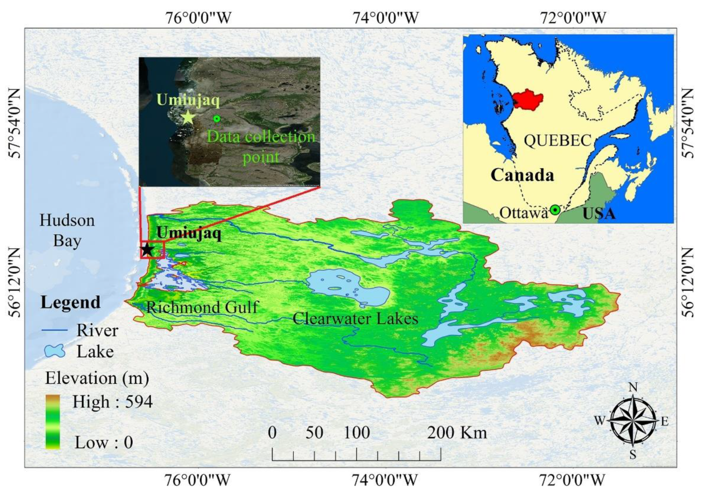
SRFD is the main component of energy exchanges between the atmosphere, the Earth’s surface, and the ocean. Therefore, it affects the context of temperature, atmospheric and oceanic circulation, and the hydrological cycle [
1]. The selected case study is located in the northern part of Quebec in Canada. The Eastern Hudson Bay Basin is situated in the east of Hudson Bay (longitudes 76°40′ W–71°30’ W and latitudes 54°50’ N–57°10’ N), which is a part of the Nunavik area (
Figure 1). Nunavik lies in both the subarctic and Arctic climate zones. Due to the climatic conditions of this area, access to the site is complex, and measuring hydrological variables in this area is not only easy but also costly. The basin’s elevation is between zero and 594 m relative to the mean sea level, and its average elevation is 300 m. The most important natural phenomena of this basin are clearwater lakes composed of two separate lakes that occupy the middle part of the basin. The deepest part of these lakes is 178 m. Annual precipitation in this basin is between 600 to 852 mm with an average of 726 mm.
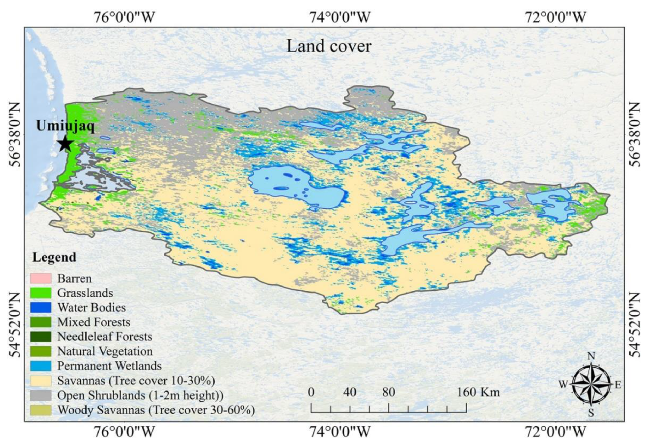
Based on land cover data (MOD12Q1, 500 m × 500 m) obtained from NASA Land Processes Distributed Active Archive Center, open shrubland mostly covers the northern parts of the area with a height of one to two meters, the southern parts mostly include savannas areas with 10% to 30% tree cover, and most of the cover is grasslands in coastal regions (
Figure 2).
Solar energy is a clean source that does not introduce any pollutants to the environment, and it may even overcome the problems caused by fossil fuels. It should be noted that this is mostly possible if the solar energy is combined with a water-energy nexus battery (e.g., hydroelectric dam) to be effective and sustainable as an energy source. In this regard, its efficient use requires practical and effective knowledge [
36]. SRFD data provide information about the impact of solar energy on the Earth in a given area over a period of time. It should be noted that due to the high cost of observing and measuring, this parameter is not easily accessible. Therefore, there is a need to create an alternative for estimating this data as well as predicting it [
37,
38]. Over the past decade, SRFD measurements as well as sunshine have declined in western Canada and elsewhere. Since the amount of SRFD is critical for calculating the evapotranspiration, soil melt, snowmelt radiation, and other hydrological cycle components, it is necessary to provide practical and accurate methods to estimate it [
39]. Because a large volume of the study area is composed of different vegetation and water, solar radiation has an influential role in the area’s environment. Changes in solar radiation in each region may affect different parameters such as plant growth period, photosynthesis, and melting outside the natural time of ice and snow (especially important due to the cold region) [
40,
41].
Since the study area is one of the cold regions and its period of frost and snowfall is high, the management of melting snow and ice is necessary for this region. Therefore, comprehension of snow and ice melting levels is essential for the proper management of available water resources, including short-term or seasonal flow forecasts, for hydrological studies and ice–snow mass balance. SRFD is an effective parameter in this regard [
42,
43].
2.2. Daymet V3 (Daily Surface Weather and Climatological Summaries)
Daymet V3 provides daily ground-level weather parameters in North America (Canada, Mexico, USA, Hawaii, and Puerto Rico) (
https://daymet.ornl.gov/, accessed on 31 March 2020). This data is available with a spatial resolution of 1000 m and a time interval of one day. Daymet includes data on daily minimum 2-meter air temperature (°C), daily maximum 2-meter air temperature (°C), precipitation, the partial pressure of water vapor, duration of the daylight period, snow water equivalent, and shortwave radiation flux [
44].
Shortwave radiation flux density (SRFD) was extracted from the gridded Daymet product for the study area. These data were processed in the Google Earth Engine environment and provide a monthly time series to apply as input in subsequent analysis. Google Earth is free, it has up-to-date maps and data, it is available on a wide array of devices, it is incredibly detailed, and it is very user-friendly. This dataset covers the period from January 1980 to December 2020. To access the SRFD data provided in the Google Earth Engine by NASA, a JavaScript-based code was offered to extract data for the desired location in Nunavik.
Google Earth Engine is a cloud platform for global spatial data analysis that allows the processing of large amounts of data in various fields, including drought, natural disaster water management, deforestation, vegetation, agriculture, soil studies, climate monitoring, and conservation of the environment [
45]. The Google Earth Engine provides convenient conditions for developing algorithms and receiving results quickly with easy access and a user-friendly environment. It improves accessibility and usability by offering Earth observation data to a wide range of research fields. Additionally, the Google Earth Engine cloud platform also provides access to relevant data and scripts for users who do not have the necessary data or computing tools [
46,
47].
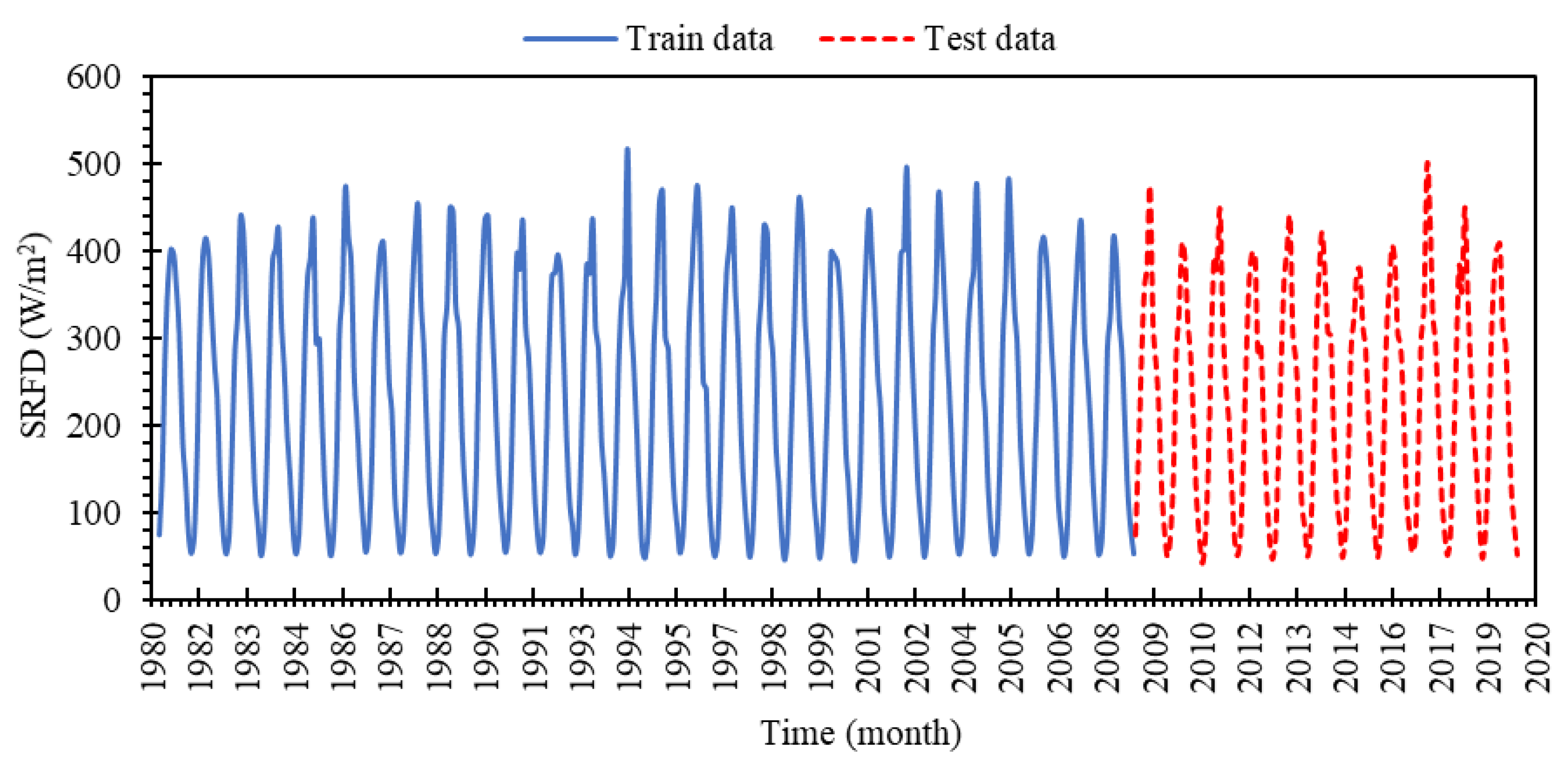
For the current study, 468 SRFD monthly data between 1981–2019 were used to model SRFD, so that 336 samples (from January 1982 to December 2008) were considered for the training phase, while the other 132 samples (from January 2009 to December 2019) were applied to check the performance of the calibrated model. The different values of the SRFD for both phases are provided in
Figure 3. Additionally, the statistical characteristics of the total, training, and testing data are presented in
Table 1.
2.3. Improved Extreme Learning Machine (IELM)
The backpropagation is a well-established training algorithm for the feed-forward neural network to solve many nonlinear complex problems leading to acceptable results [
48]. However, similar to any machine learning-based approach, the BP has some drawbacks with its generalization and implementation, including local minima, learning rate, overfitting, low generalization ability [
49], and time-consuming training [
50].
To overcome the abovementioned limitations, Huang et al. [
30] presented the extreme learning machine (ELM) as a training algorithm for a single-layer feedforward neural network. Using ELM is so simple that no parameters need to be set other than defining the network architecture. Therefore, many of the complexities of tuning parameters in gradient algorithms are not present in this algorithm. Additionally, as the modeling speed in ELM is so high, most of the training takes a short time with a large amount of data, which is not easy to model with the classical neural network; it takes about a few minutes. Therefore, the most important advantages of this method are the least user intervention, the learning process needing a single iteration, robustness, the fast learning rate, avoiding local minimizations, high generalization, and high accuracy [
51].
The modeling process in ELM consists of three main stages: (1) random determination of input weights and bias matrices of hidden neurons, (2) calculation of the hidden layer outputs matrix using randomly generated matrices and activation function, and (3) calculation of output weights through a linear process. Accordingly, among three different matrices that need to be quantified, only the output weights are calculated analytically, and the other two matrices are randomly set. The least-square solution of a linear system is considered to define the output weights matrix.
To model a problem, it is first necessary to specify the inputs and outputs of the problem. For the input matrix with d independent inputs and the output of the problem with m, the outputs are
and
, respectively. The number of S training samples are defined as
. By considering the f(·) as activation function and NHN as number of hidden neurons, the output of the feedforward neural network is considered as follows:
where NHN is the number of hidden neurons, S is the number of training samples,
is the output weight matrix that connects the jth hidden node to the corresponding hidden node, z is the number of the output variable, and O
i and InV
i are the output and input variables, respectively.
is the bias of the jth hidden neuron, and
is the input weights that link the input variables to the jth hidden node and
denotes the inner product of the a
j and InV
i. The mathematical form of the different activations applied in the current study are as follows:
Triangular Basis Function
The matrix-based form of Equation (1) with N separated equations is defined as follows:
where T, β, and O
denote hidden neurons’ output, output weight, and output, respectively. The hidden neurons output matrix (T) is defined as follows:
The two matrices T and β in Equation (8) are unknown. The H is calculated using input weights and the bias of hidden neuron matrices that both of them are randomly assigned. Therefore, T is calculated without the experience of training samples. Consequently, the output weights matrix (β) is the only unknown matrix that should be calculated through the training phase. To find this matrix, Equation (8) as a linear system should be solved.
The dimension of the T is DM × NHN. The NHN is generally higher than the input variables (DM), and therefore, the H is not a square matrix. Thus, finding the output weights matrix using Equation (8) is not simple [
30]. To find the output weights matrix, the optimal least square solution of the output weights matrix by loss function minimization is calculated as follows:
where the output weights matrix calculated through the least square solution of the above equation is calculated as:
where T
+ denotes the Moore–Penrose generalized inverse of the T [
52]. The solution of Equation (10) for NHN < S is as follows:
The dimensions of the bias of hidden neurons, input weights, and output weights matrices are “1 × NHN”, “DM × NHN”, and “1 × NHN”, respectively. Therefore, the number of all tuned parameters through the training phase of the ELM is as follows:
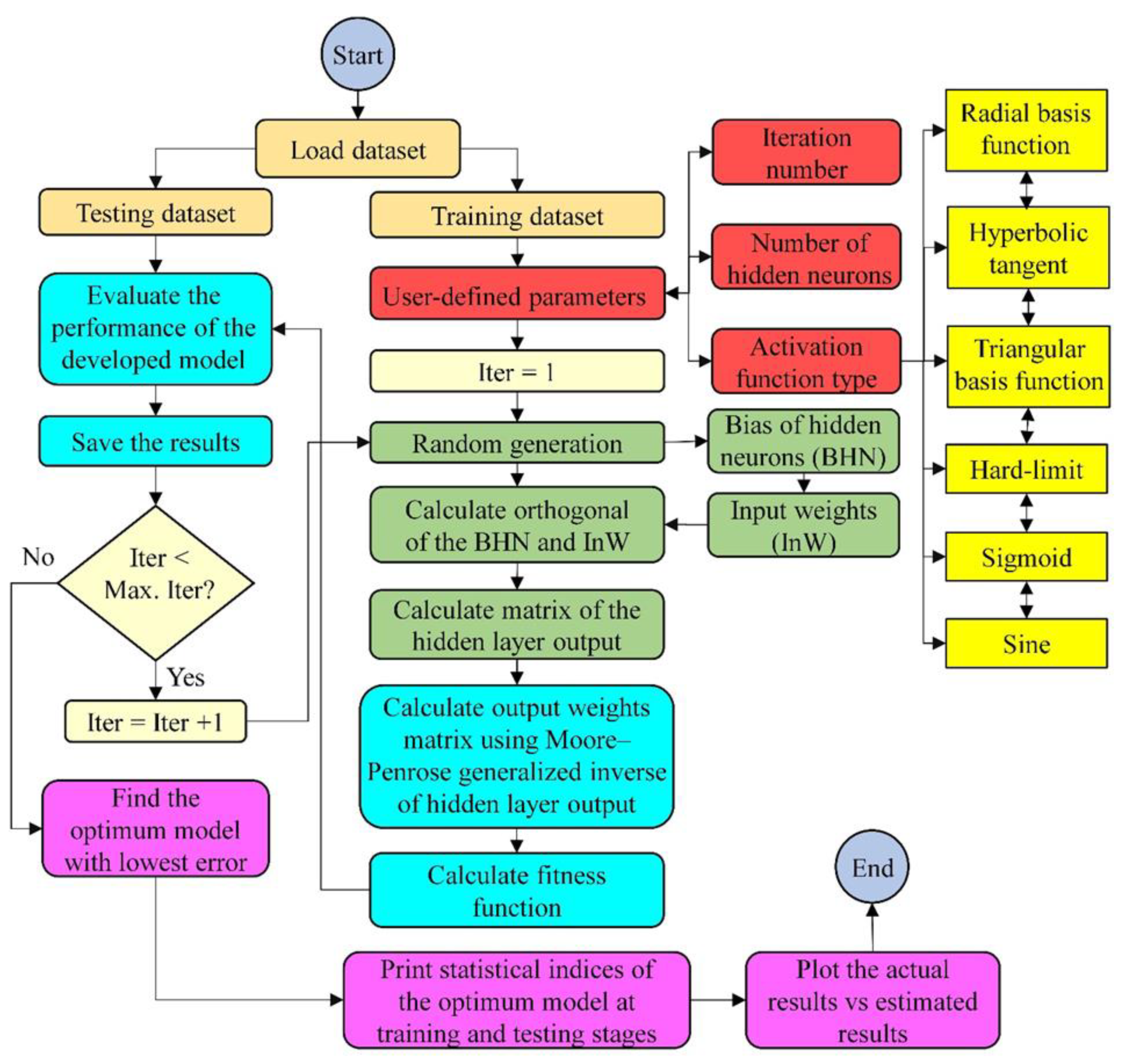
The ratio of the randomly generated parameters that are related to the input weights (i.e., DM × NHN) and bias of hidden neurons (i.e., 1 × NHN) to the output weight (i.e., 1 × NHN) is as follows:
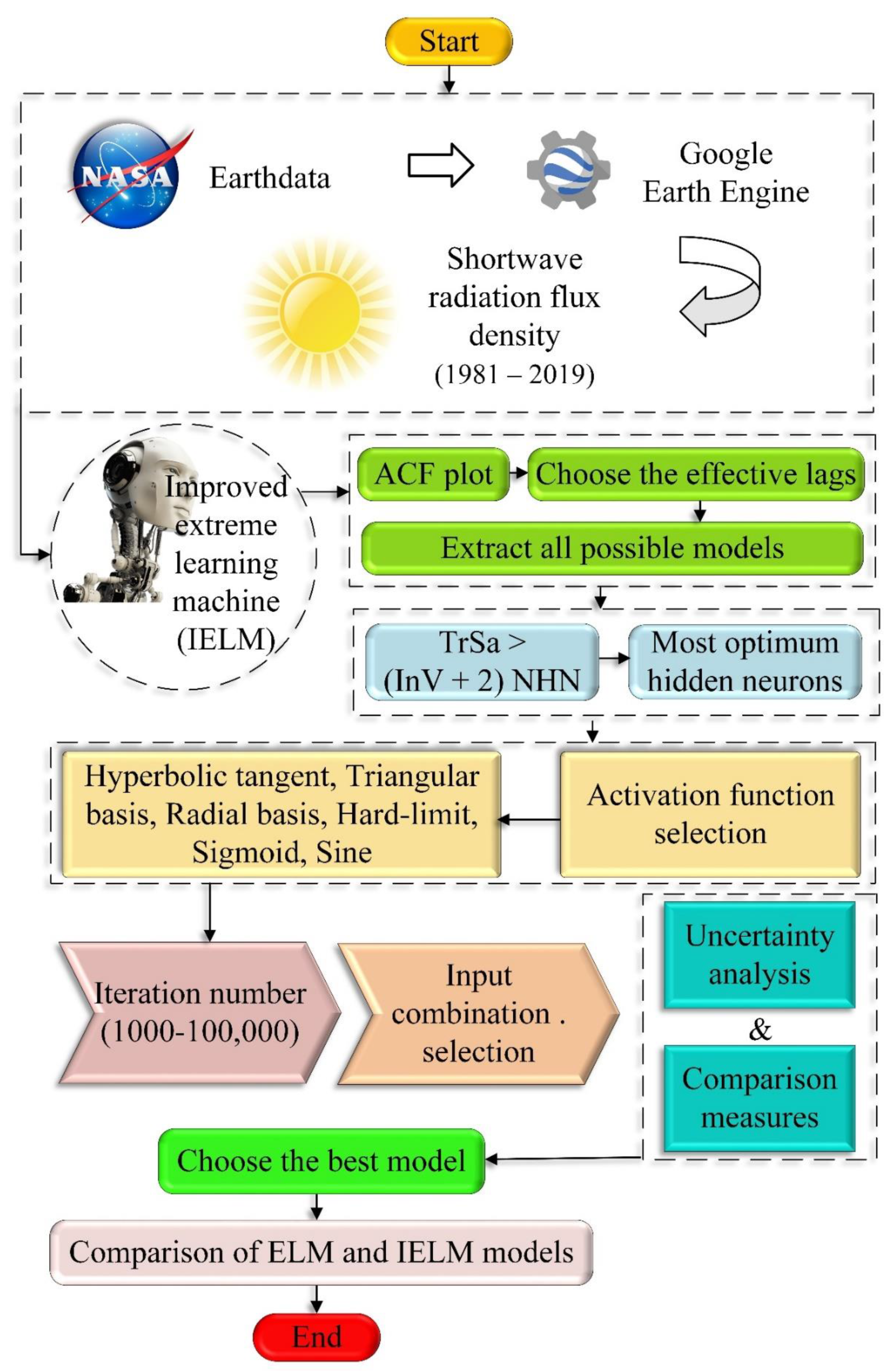
If the number of input variables is one, the R is more than 0.66. Therefore, it is observed that two-thirds of the parameters tuned in the modeling using ELM are randomly determined, which has a significant impact on the modeling results. An inaccurate value of these parameters may reduce the generalizability of the developed model. Therefore, in this study, two competencies are performed on the original ELM: (1) considering iteration parameter for ELM and (2) applying the orthonormal basis for the range of input weights and bias of hidden neuron matrices. Using these two competencies, the new version of the ELM is named improved ELM (IELM). The flowchart of the developed IELM is presented in
Figure 4.
2.4. Uncertainty Analysis
The quantitative appraisal of the uncertainty analysis (UA) in the estimation of the shortwave radiation flux density (SRFD) has employed the developed improved extreme learning machine (IELM) instead of the original ELM. For a fair comparison of the different IELM-based models, the UA is utilized to the test data [
53,
54]. The use of test data in calculating and checking the UA of the developed IELM model has the advantage that its performance is examined for testing data without any role in model training. The generalizability of this model can be confirmed. The first step in UA is the calculation of the individual estimation error (IEE) as follows:
where SRFD
E,i, and SRFD
O,i are ith estimated and observed SRFD, respectively, and E
i is the IEE of the ith sample. The IEE for all samples are applied to calculate mean estimation error (MEE) as follows:
where
is the MEE and S is the number of samples. Using the calculated
and IEE for all samples (E
i), the standard deviation of the estimation error (SDEE) is calculated as follows:
The negative (or positive) value of the MEE demonstrates that the estimator model underestimated (or overestimated) the observed values of the SRFD. To approximate a confidence band around the estimated values of an error, the ±1.96 SDEE is calculated.
2.5. Workflow Approach
In this section, the workflow approach of the current study is presented. This workflow comprises four main steps: data collecting, model definition, tuning IELM parameters, and performance evaluation. Performing all four steps will lead to achieving the optimal model in SRFD estimation.
The first step is collecting data. To collect data, SRFD is extracted from the Daymet dataset by developing a JavaScript-based code in Google Engine Cloud. Using the developed code, the daily SRFD dataset from January 1981 to December 2019 is selected. The second step is the definition of the inputs to apply developed IELM-based MATLAB code to SRFD estimation. To do that, the auto-correlation function is employed [
55]. Using this function, the most effective lags of the SRFD are found and defined as different combinations of these lags to find the best model. The third step is the definition of IELM parameters for all input combinations, defined in the previous step. To define IELM parameters, the type of activation function, the number of hidden neurons, and iteration number must be pre-defined by the user. It should be noted that the maximum number of hidden neurons should be considered. As the maximum allowable value of the hidden neurons should be considered, the number of optimal tuning parameters through the training phase will be less than the training samples. According to that, the number of columns and rows in the input weighs is identical to the number of input variables (InV) and the number of hidden neurons (NHN), respectively. The bias of hidden neurons (BHN) and output weights are two matrices with one column in which the number of rows is equal to NHN. The maximum allowable NHN is calculated as follows:
where TrSa is the number of training samples.
Besides the maximum allowable NHN, the activation function type and iteration numbers also must be pre-defined. The iteration number is considered in the range of 100 to 100,000. At the same time, the six different activation functions, including hyperbolic tangent, Sigmoid, hard limit, Sin, radial basis function, and triangular basis function, are investigated to find the optimum one. The final step of the IELM modeling is the performance evaluation of the developed models to find the optimum one. In this step, different statistical indices and uncertainty analysis are employed to find the optimum one. The schematic workflow for shortwave radiation flux density modeling is provided in
Figure 5.
2.6. Comparison Measures
In this section, four different statistical indices, including correlation coefficient (R), root mean squared error (RMSE), mean absolute percentage error (MAPE), and Nash–Sutcliffe model efficiency coefficient (NSE), are used to assess the performance of the developed IELM model in SRFD estimation. The RMSE index is of considerable importance in studying environmental and climatic parameters and is widely used in these fields [
56]. However, this index is not practical enough to check the average performance of a model, which may be a misleading index of the average error [
57]. Scale dependency is one of the main drawbacks of RSME, allowing outliers to have a significant impact on the obtained results of this index, which will make it difficult to evaluate the model, and any fraction of the data will cause fundamental changes in the results [
58]. Therefore, it is necessary to use other indices along with it. Scholars often employ MAPE because of its intuitive understanding in terms of relative error [
59]. In addition to these two relative (MAPE) and absolute (RMSE) indices, two correlation-based indices (i.e., R and NSE) are also used. According to the characteristics of each indicator, their simultaneous application can be an excellent approach to assess the efficiency of the developed IELM-based models in SRFD estimation. The mathematical definition of the R, RMSE, MAPE, and NSE is defined as follows:
where SRFD
O,i and SRFD
E,i are the observed and estimated values of the ith samples of the SRFD, respectively, N is the number of samples, and
and
are the mean of the observed and estimated SRFD, respectively.
3. Results and Discussion
3.1. SRFD Modeling
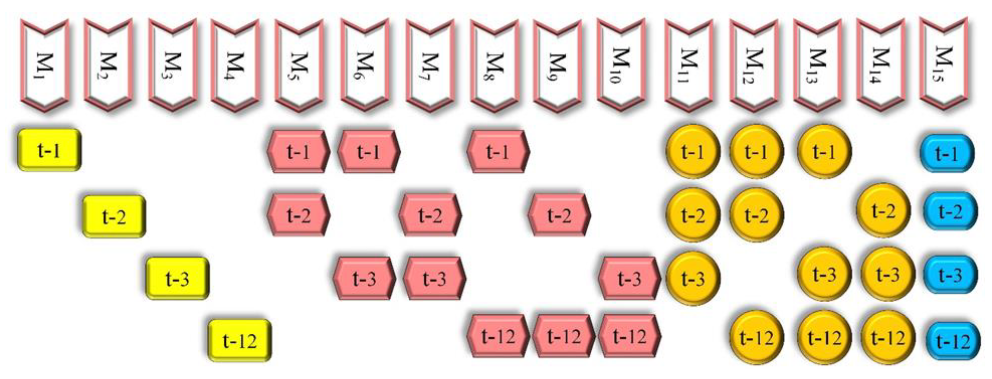
Before starting the modeling, the input parameters need to be determined. In the current study, historical values of the SRFD are used to estimate this parameter at future times. Indeed, the time series concept is used to solve the problem. Hence, effective lags are determined using the auto-correlation function. It indicates the correlations between the past and future values of the desired parameters (i.e., SRFD in the current study). The auto-correlation function of the SRFD time series was shown the most critical lags are 1 and 2. Additionally, Lag 12 is also evident as the periodic term. In addition to these three lags and to find a more reliable model, Lag 3 is also considered as one of the input parameters in the IELM-based modeling:
According to the above equation, the number of fifteen input combinations with one to four input variables is defined as provided in
Figure 6.
3.2. Most Optimum Hidden Neurons
After defining different input combinations, finding the optimal number of neurons for SRFD estimation is required. For this purpose, Model 15 with SRFD (t − 1), SRFD (t − 2), SRFD (t − 3), and SRFD (t − 12) as input parameters (
Figure 6) is employed. Additionally, by keeping other tuning parameters constant, including the activation function (i.e., Sigmoid) and iteration number (10,000 iterations), the optimal number of neurons is found. It should be noted that this number can be changed in the range of 1 to Max. NHN (Equation (18)). The reason for limiting the number of hidden layer neurons to Max is that increasing NHN could result in higher generalizability of the model so that if this limitation is not taken into account, the generalizability of this model may be doubtful.
The total number of data is 468, 70% of which have been selected as training samples, and 30% of the samples were considered testing samples. Taking into account the delays created in the modeling process, the value of TrSa is 336 (this number can be varied by changing the inputs). Given that the modeling process was initially performed using all lags (Model 15), the value of InV is equal to four. Consequently, the Max. NHN is calculated as 55 (Equation (18)).
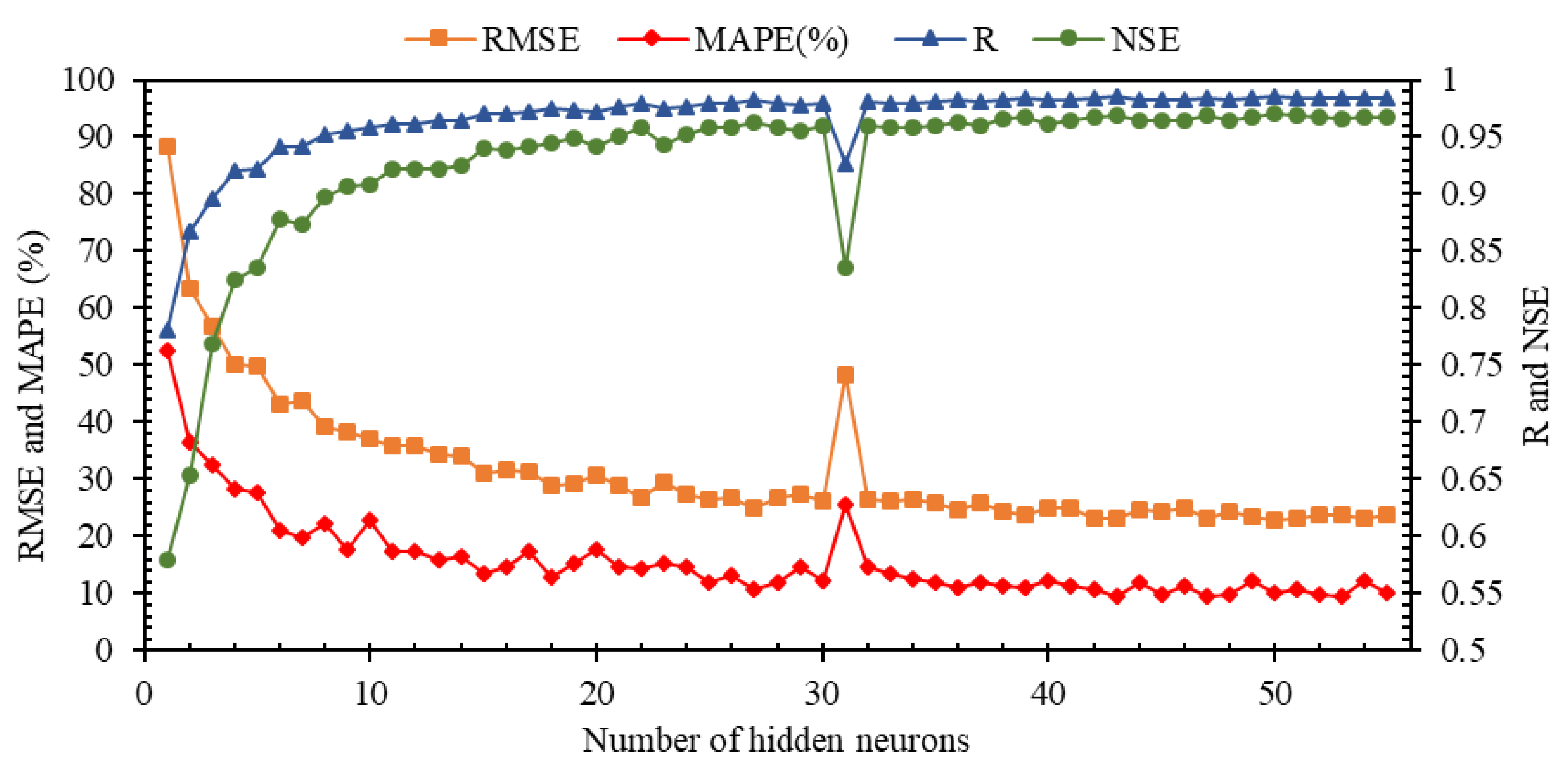
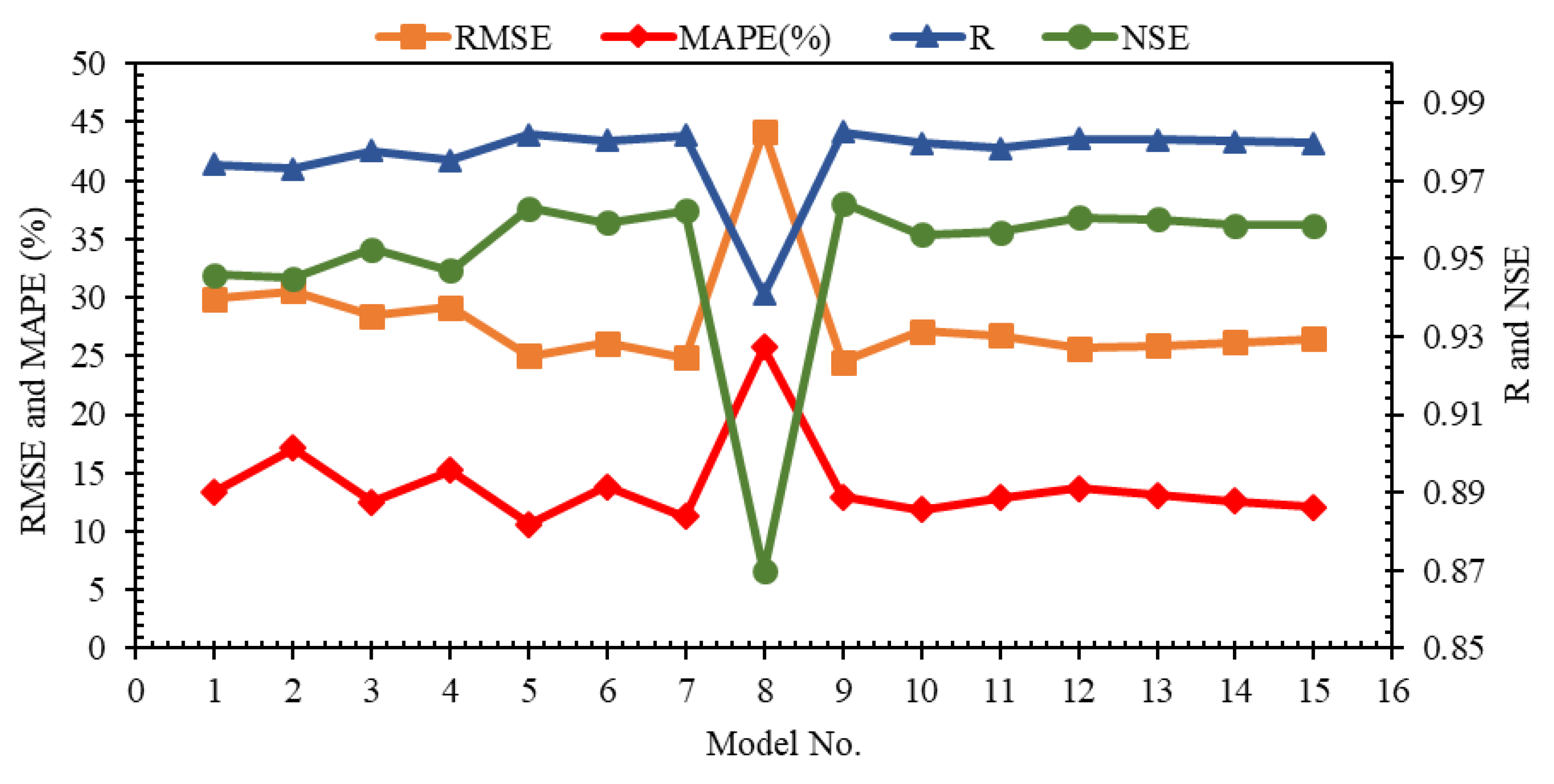
The statistical indices of the developed IELM with different hidden neurons are provided in
Figure 7. The minimum values of NSE and R are less than 0.6 and 0.8, respectively. As the number of the hidden layer neurons increases, the value of these two indices increases significantly. In NHN > 10, the value of both indices is more than 0.9, which is an acceptable value. Although the growth of the value of these two indices is also observed in most models with NHN > 10, the growth rate compared to NHN < 10 has a significant decrease. The upward trend presented in the correlation-based indices (i.e., R and NSE) is also observed as a similar downward trend in RMSE and MAPE (%). A significant point is a sharp decrease in the value of R and NSE as well as the increase in the RMSE and MAPE (%) at NHN = 31, which is significantly different from the values of its neighbors. One of the reasons for the performance of Model 31 may be the number of iterations, so for this model, the number of more iterations was examined, but there was no effective change in the performance of the model in the testing stage. Another reason can be the lack of accurate assignment of the input weights and bias of hidden neuron parameters, which has led to a significant reduction in the generalizability of this model. The results of this figure show that the best performance is obtained at NHN = 27 (R = 0.98; NSE = 0.96, RMSE = 25.02; MAPE (%) = 10.64). Therefore, the number of hidden neurons in the following modeling process is considered to be 27.
3.3. Activation Function Selection
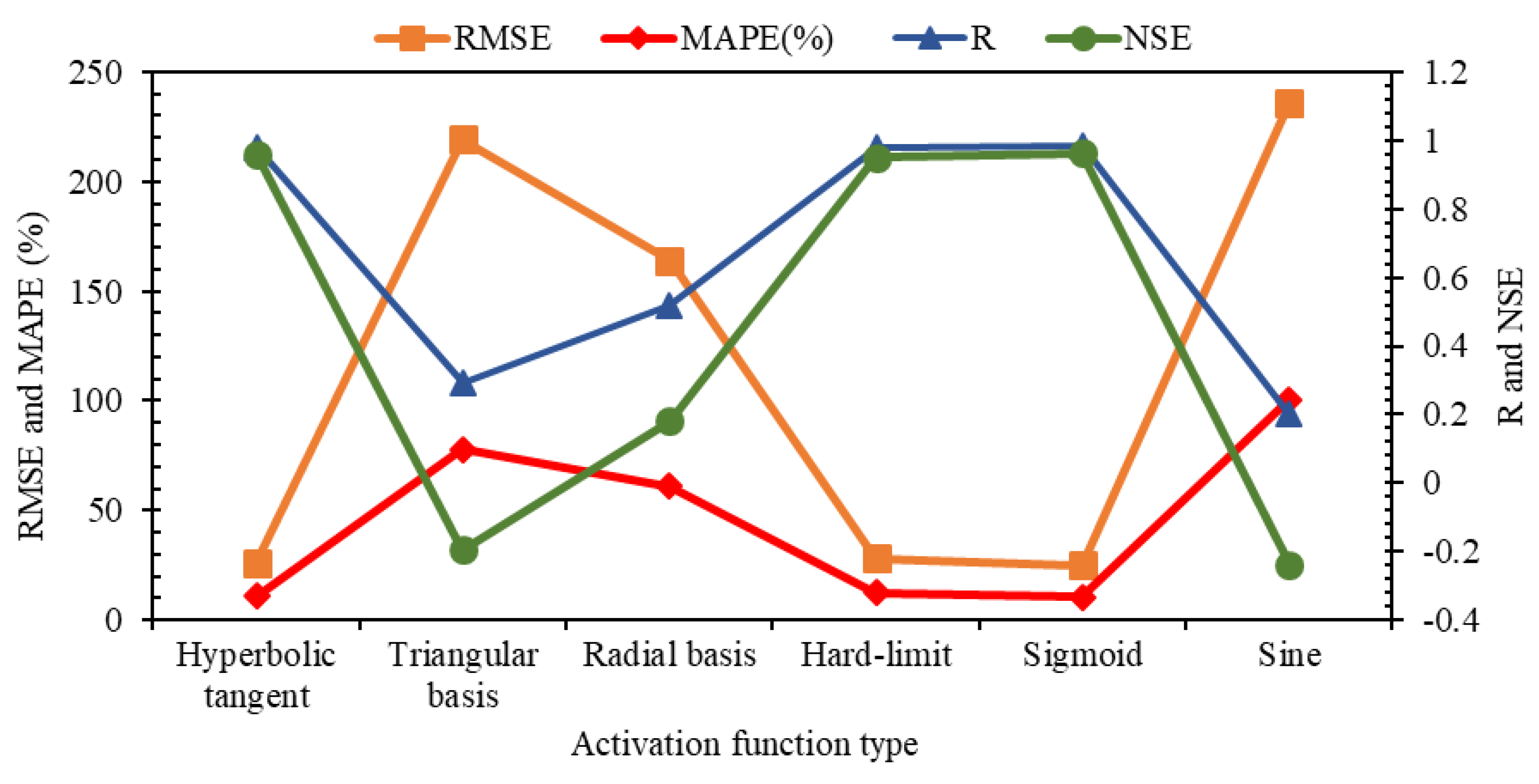
After determining the optimum number of hidden neurons, six activation functions, including hyperbolic tangent, sigmoid, radial basis function, triangular basis, hard limit, and sine, are evaluated in this section. The statistical indices of the IELM with defined input combinations in Model 15 and different activation functions are provided in
Figure 8. As shown in this figure, although hyperbolic tangent, hard-limit, and sigmoid activation functions have close results, the RMSE value for sigmoid is improved by 12.2% and 4.2% compared to hard-limit and hyperbolic tangent, respectively, which indicates sigmoid function performs better than the other two functions. The RMSE for the other three functions (i.e., sine, radial basis, and triangular basis) is about ten times the value of this index for sigmoid. Moreover, the value of MAPE error index for sigmoid is 10.64% and for hard limit and hyperbolic tangent functions are equal to 12.44% and 11%, respectively. The NSE index shows the same results for the three mentioned activation functions. Additionally, the correlation coefficient value indicates the equality of this index in the hyperbolic tangent and sigmoid functions with a value of 0.98, while this value for the hard limit is 0.97. Therefore, it can be concluded that sigmoid has shown better performance compared to the other activation functions.
3.4. Iteration Number
The third parameter is used to determine the iteration number. Many iterations in IELM modeling are used to overcome the problems caused by randomly determining the two matrices of bias of hidden neurons and input weights, which include at least 66% of the total parameters optimized during the training process (Equation (14)).
In the next step, the effect of iteration number in SRFD modeling was investigated. To investigate the impact of changes in the iteration number, a boxplot diagram was used to obtain the best number of iterations in the modeling process. In this study, 15 different values were used for the iteration number in the range of 10,000–100,000, similar to
Table 2. The distribution of RMSE values for various iterations is shown in
Figure 9. According to the high value of RMSE for some models, the maximum value of RMSE in this figure was plotted in two ranges, [0, 2×10
7] and [0, 160]. Additionally, the boxplot parameters, including minimum, maximum, median, first quartile (Q1), and third quartile (Q3), are provided in
Table 2. The difference between Q1 and Q3 is known as IQR. Using IQR, the minimum and maximum values are calculated as Q1 − 1.5 × IQR and Q3 + 1.5 × IQR, respectively. Values smaller than the minimum and larger than the maximum are known as outliers. Indeed, if a number outside this range is recorded, it indicates that the amount of model error that is considered as RMSE in some cases might be very small or very large.
Figure 9 shows that at iteration number = 30,000, the RMSE value also reaches 2×10-
7, a high value for this index. By limiting the error range to [0, 160], it can be seen that in all the values defined for the iteration number, a very large number of iterations record an error value greater than the maximum value (=Q3 + 1.5 Q IQR). Except for iteration numbers = 10,000 and 30,000, in other cases, the changes’ range minimum, maximum, Q1, and Q3 are almost constant.
In Model 5 (iteration number = 10,000), the median is 62.4, which indicates that 50% of the data model from 10,000 runs is in the range of 47.64 to 81.13, while the lowest error recorded in this case is equal to 21.11. In all other models with different iteration numbers, the minimum error value is greater than 21.11, which indicates the better performance of Model 5 (
Figure 9).
Figure 10 signifies the statistical indices of the best IELM-based model with the different iteration numbers. According to this figure, the lowest MAPE (%) was recorded for the iteration number = 10,000 (MAPE (%) = 10.64). The correlation-based indices (i.e., R and NSE) for all iteration numbers except 30,000 are very close together. The lowest and highest values of R are 0.973 and 0.982, respectively, and the lowest and highest of the NSE are 0.945 and 0.964, respectively. The lowest RMSE is related to the 20,000 iteration (RMSE = 24.83). Considering the values of different indices, the iteration number = 10,000 is selected as the optimum value of the iteration number (R = 0.98, NSE = 0.96, RMSE = 25.02, and MAPE (%) = 10.64).
3.5. Input Combination Selection
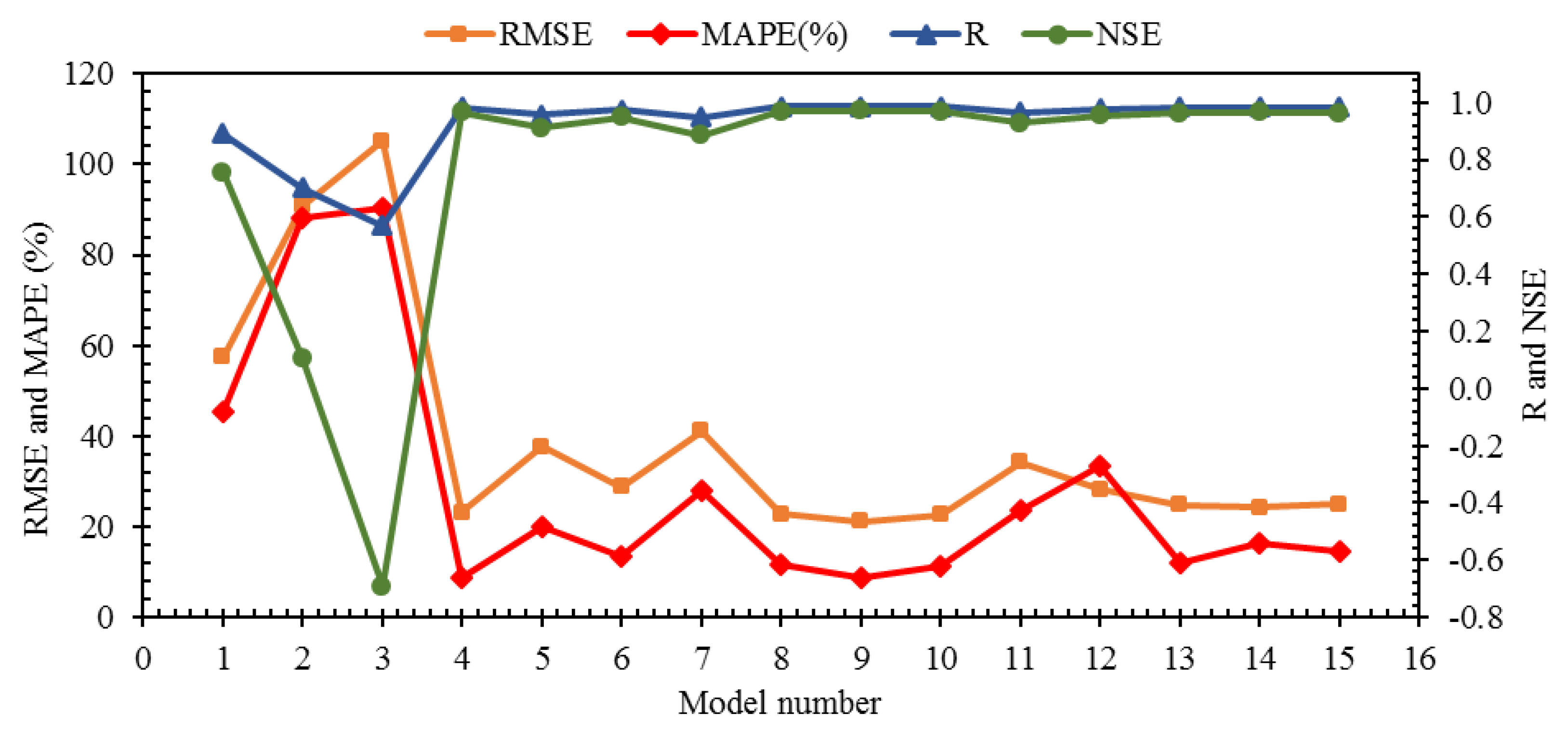
After determining the modeling parameters in IELM, the effect of each input is examined by considering 15 input combinations, defined in
Figure 6. The presented models in this figure are divided into four general categories: models with one, two, three, and four inputs, which include four, five, four, and one input combinations, respectively.
Models 1 to 4 are single-input models that include Lag 1, 2, 3, and 12. Among the models presented with a single input, it is observed that the highest value of correlation-based indices (i.e., R and NSE) is related to Model 4 (R = 0.983, NSE = 0.966) so that the closest value of these two indices to Model 4 corresponds to Model 1 (R = 0.892; NSE = 0.756). The results of these two indices in Lag 2 and Lag 3 are significantly different from the other two lags because in Lag 3, the NSE index has a negative value (NSE = -0.691). The value of this index in Lag 2 (NSE = 0.106) is approximately 10% of the value of this index in Lag 12. In addition to these two indices, Model 4 (i.e., Lag 12) also offers the best performance in RMSE and MAPE indices, so that the modeling relative error is less than 9% (MAPE (%) = 8.88), while the value of this index for Models 2 and 3, whose inputs are Lag 2 (MAPE (%) = 88.23) and Lag 3 (MAPE (%) = 90.28), is about ten times the value of this index in Model 4. According to the explanations provided, Lag 12 has the most effectiveness, and Lag 1 is in the second place for one-step-ahead modeling of SRFD by considering only one lag.
Although Lag 2 had the weakest performance among all lags, its combination with Lag 1 (Model 5) (R = 0.956; RMSE = 37.645; MAPE (%) = 20.038; 0.911) increased the performance of Model 1, which uses only Lag 1 so that the values of R, RMSE, MAPE, and NSE indices have increased by 7.24%, 34.42%, 55.88%, and 20.47%, respectively, compared to Model 1.
The combination of Lag 3 with Lag 1 has also led to Model 6 (R = 0.975; RMSE = 28.833; MAPE (%) = 13.352; 0.948), which is more accurate than Model 1. According to the results presented for single-input models, the weakest performance was observed for Lag 3. Therefore, it was expected that using Lag 2 in combination with Lag 1 would provide better performance than combining Lag 3 with Lag 1, but Model 6, whose inputs are Lag 1 and Lag 3, compared to Model 5, whose inputs are Lag 1 and Lag 2, provided better performance. Therefore, it is concluded that to achieve the optimal model, it is necessary to examine the synergy of different parameters with each other.
Considering that in single-input models, the best performance was obtained for Lag 12, which was significantly different from other lags, it is expected that the combination of this lag with one of the other lags (i.e., Lags 1, 2, and 3 as Models 8 to 10, respectively) leads to a more accurate result compared to Models 5 to 7. The results presented in
Figure 11 show that the performance of Model 4, whose only input was Lag 12, has been slightly improved by Models 8 to 10 (two-input models). In Models 8 to 12, correlation based-indices (i.e., R and NSE) and RMSE experienced an increase in accuracy compared to Model 4, which has only one input (i.e., Lag 12). Still, for MAPE, this trend is not incremental in all three models. In Models 8 and 10, which use Lag 1 and Lag 3 (respectively) as input in addition to Lag 12, the MAPE is increased by about 2.5%, while in Model 9, which uses Lags 2 and 12 to estimate SRFD, the value of this index has decreased. Therefore, it is concluded that the simultaneous combination of Lag 12 and Lag 2 offers the best performance between models with 1 to 2 inputs. As the number of model inputs increases to 3 and 4 (Models 11 to 15), it is observed that in all models, correlation-based indices decrease, and both RMSE and MAPE indices are increased. Therefore, it is concluded that Model 9 is the best input combination for SRFD estimation.
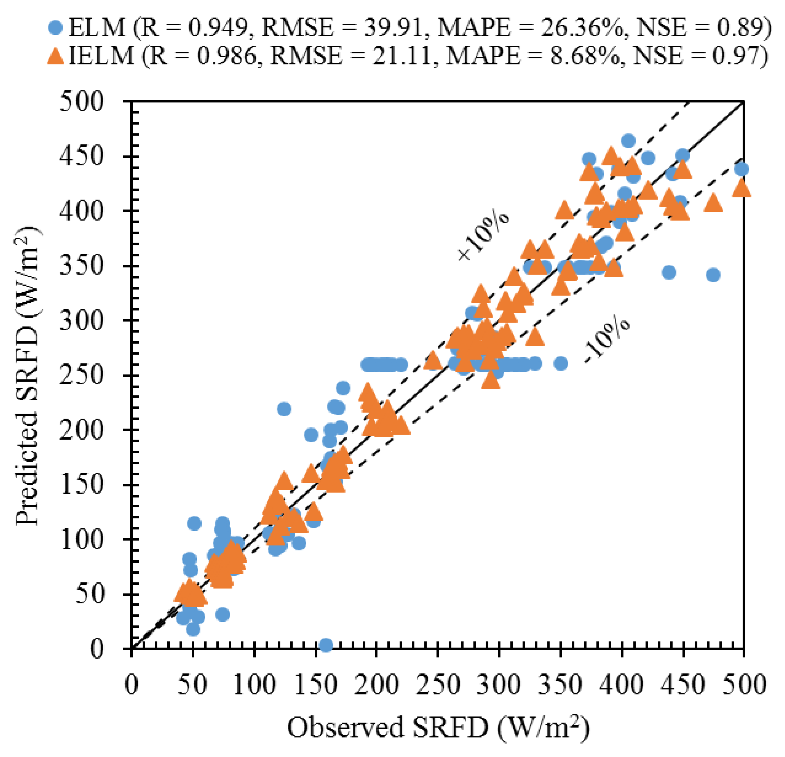
3.6. Comparison of the IELM with ELM
Figure 12 illustrates the scatter plot of the observed and predicted SRFD by ELM and IELM. According to this figure, most of the estimated samples by IELM are in the range of ±10%, while the results provided by ELM in different SRFD ranges have many errors. Most of the estimated samples by the ELM in the range of 180–350 are fixed so that in this range, the estimated points do not follow the 45-degree line and are presented almost in a horizontal line.
In both ELM and IELM methods, the errors are presented in both under and overestimate forms, and the only significant difference is the modeling error values. The indices presented in the figure show that correlation-based indices (i.e., R and NSE) in the IELM method have increased by about 3.9% and 9% compared to ELM. An increase of about 47% and more than 17% was observed in RMSE and MAPE, respectively. Therefore, it is determined that the developed method in the current study (i.e., IELM) has well overcome the limitations of the ELM method.
3.7. Uncertainty Analysis of the IELM Models Versus ELM
The uncertainty analysis (UA) results are summarized in
Table 3. The mean estimation error (MEE), standard deviation of estimation error (SDEE), 95% estimation error interval (EEI), and width of uncertainty band (WUB) are provided in this table. According to this table, the MEE for IELM
4 and ELM are positive, while the value of this index for others is negative. Therefore, it is concluded that these two models over-estimated the SRFD, while the other models underestimated the SRFD. Given that the positive and negative values of the error are added together by considering their sign, the use of this model cannot be used as an index to check the accuracy of the model. Therefore, other indices need to be evaluated. The SDEE for all IELM models indicates that this index’s lowest and highest values are associated with 21.12 and 105.47, related to the IELM
9 and IELM
3, respectively. The widths of uncertainty bands of the IELM are in the ranges of [±17.56, ±3.64] so that the lowest and highest ones are related to the IELM
3 and IELM
9, respectively. The widths of uncertainty bands for ELM is ±6.9, which is 52% higher than the best of the IELM model (WUB (IELM
9) = ±3.64).
The universal form of the IELM is as follows:
where the InW, InV, BHN, and OutW are the input weights, input variables, bias of hidden neurons, and output weights, respectively. The InW, InV, BHN, and OutW are defined as follows:
4. Conclusions
Shortwave radiation flux density (SRFD) modeling can be a key factor in the better control of environmental parameters such as evaporation, transpiration, use in solar structures, etc. In the current study, an improved version of the ELM (IELM) is proposed to overcome the limitation of this method due to random generation of the two matrices, including input weights and bias of hidden neurons. Additionally, the Google Earth Engine environment is employed to extract the monthly satellite-based data of the SRFD from the gridded Daymet product. The datasets were from January 1981 to December 2019. Because the time series concept was used in the SRFD modeling, using the SRFD historical data, the most important lags were found to determine the input combinations. The auto-correlation function was applied to find the most effective lags. This function indicated that Lags 1, 2, 3, and 12 are the most effective ones. Using these lags, fifteen different input combinations were obtained. The best input combination was found through the modeling phase, with Lags 2 and 12 as input variables. It should be noted that the sigmoid was found as the best activation function, and the optimum number of hidden neurons was 27. By considering different iteration numbers from 1000 to 100,000, the best results were obtained at 10,000. Comparison of the developed IELM (R = 0.986, RMSE = 21.11, MAPE = 8.68%, NSE = 0.97) with original ELM (R = 0.949, RMSE = 39.91, MAPE = 26.36%, NSE = 0.89) proved the higher performance of the developed ones. Additionally, the uncertainty analysis results indicated that the widths of uncertainty bands for IELM (WUB = ±3.64) are almost half of this index’s calculated value for the original ELM (WUB = ±6.9). A matrix-based equation for the optimum IELM-based model is provided to calculate SRFD for one month ahead using Lags 2 and 12. Using this model in predicting the amount of SRFD can be a practical solution in energy and water resources management. In the current situation, where environmental factors and climate change are occurring, using this type of model can be an effective way to advance the management of goals and achieve a roadmap in the future with a sustainable development approach. In the current study, the developed model was checked for only one station. The developed IELM could be applied to other stations and other real-world problems. The developed IELM applied an iterative process to overcome the limitation of the classical ELM in random generation of the two main matrices (i.e., input weights and bias of hidden neurons). However, an implementation of the developed ELM to overcome the mentioned drawback could also be made in a follow-up study by using the new developed evolutionary algorithms such as sperm swarm optimization (SSO), conscious neighborhood-based crow search algorithm (CCSA), and other evolutionary-based algorithms to optimize the randomly generated parameters for the input weights and bias of hidden neurons matrices. Moreover, the ACF was applied to track the most effective lags dependence structure of the SRFD. As the ACF has a large statistical bias that tends to underestimate the second-order dependence structure, it is recommended to apply alternative methods.


 ,
, 


