Dynamic Effect of Oil Resources on Environmental Quality: Testing the Environmental Kuznets Curve Hypothesis for Selected African Countries

Abstract

This paper examines the environmental Kuznets curve (EKC) theory, augmenting the role of oil resources and energy consumption in carbon dioxide (CO₂) emissions using the annual data of 11 African oil-producing countries from 1980 to 2014. We apply advanced panel cointegration and panel autoregressive distributive lag (ARDL) techniques coupled with Granger non-causality analysis to account for cross-sectional dependence and heterogeneity. The results of the augmented mean group (AMG) reveal that oil resources abundance degrades the environmental quality in Angola while abating CO₂ emissions in Algeria, Gabon, Morocco, and Nigeria. Contrarily, energy consumption escalates pollution in the Congo Democratic Republic (COD), Côte d’Ivoire (CIV), Gabon, Morocco, and Tunisia. Our findings support the EKC hypothesis only in Cameroon, CIV, and Nigeria while exhibiting a U-shaped curve in Algeria and Morocco. Causality analysis unveils that oil resources Granger cause energy consumption, suggesting the balance between renewable and non-renewable energy sources. The current study has important policy implications for promoting green technology, economic diversification, service sector, and green investments.

1. Introduction

Sustainable development determines the future of humankind while oil resources dependence and the ongoing greenhouse gases (GHG: nitrous oxide, carbon dioxide, gas flaring, methane, etc.) emissions have severe consequences for the environment and global warming [1,2,3,4,5,6,7]. In a recent study, Gatto et al. [8] report that oil-dependent developing and emerging countries share 15–20% of GHG emissions in the Earth’s atmosphere. As documented in the Climate Watch [9], carbon dioxide (CO₂), with a share of 74% in GHG emissions in 2017, remains the main component of environmental degradation and climate change. For example, in 2016, the oil-based activities sourced 12.3 billion metric tons (or 30%) of the planet’s CO₂ releases [10].

In this context, Africa is the lower-emissions region with a share of only 4% of carbon release from the world fossil fuel sector in 2017 [11]. The region also accounts for over one-third of carbon pollution from energy use and manufacturing sector compared to 80% of such emissions worldwide, while this continent is the most vulnerable to global warming [3,12,13,14]. African economies have also experienced one of the world’s highest levels of gross domestic product (GDP) growth of 4.5% for almost two decades (1995–2013), which persisted even during the 2008/2009 financial crisis [15,16]. Oil resources abundance is the backbone of economies in countries such as Nigeria and the Congo Democratic Republic (COD), with around 5.8% and 5.9% average annual GDP growth over 2000–2019 [17]. Additionally, according to World Bank [17], the GDP figures for African region (expressed in constant 2010 US dollars ($)) amounted to $664.583 billion, $812.256 billion, and $1.834 trillion in 1990, 2000, and 2019, respectively. The corresponding average annual growth has been 2.2% (for the first decade 1990–2000) and even more vigorous with 4.6% (for the following two decades 2000–2019). United Nations Economic Commission for Africa (UNECA) [18] and Talukdar and Meisner [19] show concerns because these growth trends could have the adverse environmental impacts. Meanwhile, Africa with its infant industries, including oil companies, also became greater CO₂ emitter due to the overextraction of oil resources (to support the said growth); the oil processing requires extensive energy use, resulting in fugitive emissions, etc. [4,13,18,20,21,22]. According to the International Energy Agency (IEA) [23], the economic growth and oil resources dependency has raised the energy demand up to 80% of the total energy required to stimulate the region’s economic activities. The 2020 report of British Petroleum (BP) [24] revealed that fossil fuel energy consumption in Africa, including oil resources, amounted to over 40% of the total energy mix. Such an extensive use of primary energy had a detrimental effect on the environment [25,26]. Though Africa is the least carbon polluter of the planet, yet its carbon emissions are increasing over the years. In this regard, BP [24] draws the attention that the CO₂ emissions in the region increased from 1070.2 million tons in 2009 to 1308.5 million tons in 2019, with an annual growth of 2.0% between 2008 and 2018. These African emissions trends could even dramatically rise to 30% by 2030 with the region’s GDP and population growth projection [11].

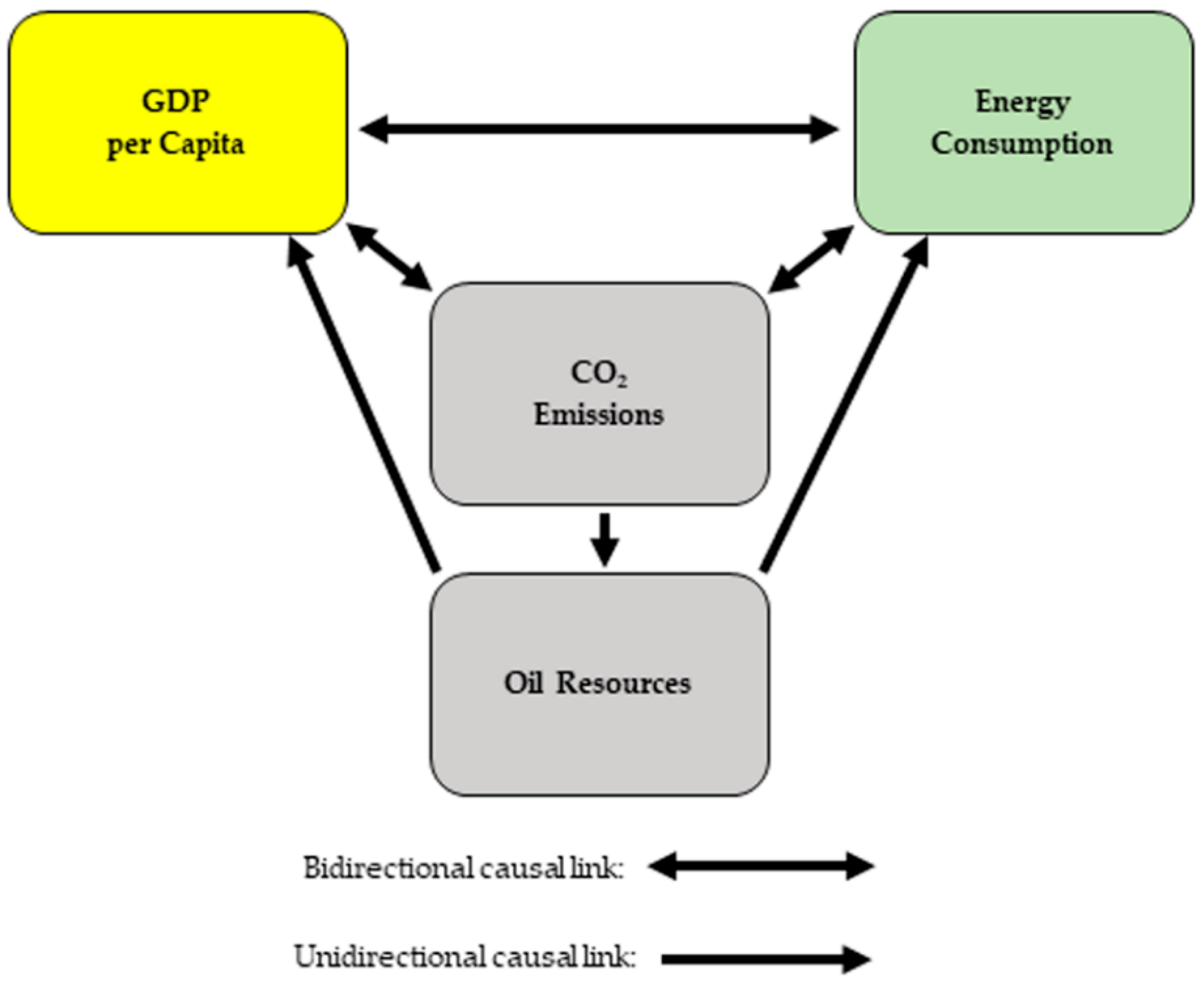
The prior literature mainly suggests an inverted U-shaped relationship between income level and pollution, commonly known as the environmental Kuznets curve (EKC) [27,28,29,30,31]. Particularly, the development level affects the environmental quality based on scale, composition, and technical (also called technique effect) effects of the economy [32]. Scale effect postulates that holding the structure and the technology of the economy unchanged, the production increase leads to environmental deterioration. Thereby, economic development worsens environmental pollutions and related climate damages [32,33]. The pre-industrial era relates to the scale effect because economic prosperity improves the living standards of people who initially consume more energy-intensive goods increasing the pollution level. Thus, IEA [34] documented the boom of fuel-based vehicles, which are the most polluting (carbon emitters). The industrialization era leads to the overexploitation of the oil resources to match the economy’s energy needs. Consequently, this operational process jeopardizes the environment by emitting CO₂ through fugitive emissions and flaring. Furthermore, the oil sector’s energy consumption, together with that of the rest of the economy, enhances the carbon emissions, ultimately damaging the environmental quality. In the second stage, additional economic growth shares a high-income level in moving from quantitative to qualitative growth. Particularly, as the economy develops, citizens may require a safe and healthy environment. This process characterizes the ongoing structural change in the economy from agricultural activities to the heavy and “dirty” industry, then to virtual activities (services): post-industrial era. The said economic transition contributes to low-pollution intensity after crossing the turning point (TP) via development of advanced and innovative technology in the economy. The aforementioned mechanism corresponds to the composition effect. Lastly, the technique effect gauges the production efficiency and the adaptability of energy-efficient and low-carbon technologies, which improves the environment [3,4,32,33,35,36,37,38,39,40]. 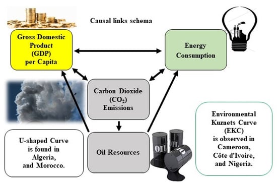Figure 1 depicts the described process comprehensively.

The past studies provide inconclusive and controversial findings about the nexus between oil production and environmental pollutions. For instance, Johnston, Lim, and Roh [5] found that oil resources exploitation degrades the air quality. Furthermore, the dependence of the economy on the fossil fuel exploitation is unfriendly to sustainable development because it boosts CO₂ and flaring emissions [20]. Extending these views, Fuinhas, et al. [41] found that oil rents increase carbon emissions in the case of 21 oil-rich economies. Similarly, Mahmood et al. [42] applied the non-linear ARDL approach to analyze Saudi Arabia’s environmental conditions. Their empirical outcomes revealed that the economic growth and oil rents positively affect the carbon footprints.

Moreover, several studies have also tested EKC hypothesis in connection with the oil-resource abundance. For instance, Mahmood and Furqan [37] investigated the connection between GDP, oil rents, urbanization, foreign direct investment, financial market development, energy consumption, and CO₂ emissions in the Gulf Cooperation Council (GCC) six economies. They confirmed the EKC hypothesis by utilizing the fixed effects (FE), and the spatial Durbin model (SDM). Additionally, energy consumption, GDP, and oil rents aggravate carbon pollution in GCC countries and even in border countries. In a similar vein, Sadik-Zada and Loewenstein [44] tested the EKC hypothesis by examining the relationship between income and carbon emissions in 37 oil-rich counties cross-time 1989–2019. Their findings confirmed an inverted U-shaped relationship between economic growth and pollution, while oil rents significantly enhance environmental pollution in oil-producing countries.

Ike et al. [45] also found an inverted U effect of economic growth on CO₂ emissions only in countries with median and higher level of carbon emissions. Moreover, from the first to sixth quantile, oil production significantly accelerates carbon emissions. However, the results are quite heterogeneous as this effect is weaker in the highest quantile and stronger in the lowest quantile. Sadik-Zada and Gatto [46] examined the EKC phenomenon in 38 oil-producing countries from 1960 to 2018 and rejected an inverted U-shaped nexus between income per capita and CO₂ emissions. They found that the tertiary or service sector increases carbon emissions by a lower rate than the manufacturing sector does (which causes three times more emissions). Therefore, the structural shift to the tertiary sector triggered by oil rents could substantially improve the environmental quality in oil-rich countries. These findings indicate the level of oil resources abundance has an asymmetric effect on the environment, which requires further inquiry in other country settings with diverse economic, geographical, social, political, and technological factors.

Some papers have also successfully tested the EKC hypothesis in African region by including additional factors. For instance, in their regional analysis, Bibi and Jamil [47] confirmed an inverted U-shaped relationship between economic growth and carbon emissions in North Africa, while their findings refuted the EKC hypothesis in Sub-Saharan Africa. Yusuf et al. [48] found the similar results in case of African oil-producing countries. While taking several measures of environmental pollution, they proved the EKC theory for methane gas emissions only. Tiba and Frikha [49] also observed a bell-shaped relationship by applying the dynamic panel models in case of 26 African countries. Mahmood et al. [50] applied the spatial analysis, in their recent study on North African region, to probe the EKC phenomenon by taking the additional factors such as imports, exports and foreign direct investment. Their findings unveiled the existence of the EKC or bell-shaped nexus between economic growth and CO₂ emissions. However, Sarkodie [51] reported mixed evidence about the EKC in Africa. Their findings revealed an inverted U-effect of economic growth on carbon emissions and a U-shaped influence of economic growth on ecological footprints.

The prior studies have mainly tested the effect of energy consumption on pollution in Africa. For example, Awodumi and Adewuyi [25] demonstrated that energy consumption promotes growth while raising CO₂ emissions in African oil-producing countries. Using the augmented mean group (AMG) model for 19 African economies, Nathaniel and Iheonu [26] affirmed that many African nations relied on energy consumption to power their economies even though the said energy source is carbon-intensive. Similarly, Muhammad [52] documented the pollution-enhancing role of energy consumption in North Africa. The past literature has mainly overlooked the underlying nexus of carbon emissions with oil resources abundance, energy consumption, and growth in Africa. To fill this gap, the objective of the current research project is to explore the effects of oil resources abundance, energy consumption, and economic development on CO₂ emissions within the EKC framework. To our best knowledge, this is a pioneering study in bridging the identified gap in the African context. It is important to examine the identified gap for Africa because, with its history of oil exploitation, the region is also identified as home to at least 30% of the world’s newly discovered oil and gas resources [23]; these African oil resources have always attracted multinational companies to invest and exploit these resources.

The study contributes to the existing literature as follows: First of all, this study is the fresh empirical evidence on the EKC hypothesis based on energy consumption and oil resources abundance in African economies. The prior studies have mainly examined the EKC hypothesis with other factors especially in Africa. Moreover, their empirical findings are highly controversial and inconclusive. Therefore, our study is the first to empirically test the linkage between oil-resource abundance and environmental quality in the context of the EKC theory. Secondly, following the study of Ulucak and Bilgili [53], we investigate the EKC hypothesis by examining the role of development level in explaining the heterogeneous relationship between income level and pollution. Therefore, we divided our data into two panels, namely, lower-middle income and low-income (LMI and LI) and upper-middle income countries (UMI) based on income-group classification of the World Bank. Thirdly, we determine the TP of the EKC results to find out the threshold levels of specific African economies for policy formulation. Fourthly, the study applies the advanced panel ARDL model, AMG, to account for cross-sectional dependence (CD) and sample heterogeneity problems, which have been ignored in some past studies. Lastly, we apply the Dumitrescu and Hurlin (D–H) Granger non-causality approach as an additional robustness measure to determine the causal linkages among our considered variables. Based on this empirical analysis, the findings would extend the existing literature and provide a reliable roadmap to policymakers for sustainable development and ecological balance, not just the economy.

2. Methodology

2.1. Model Construction

The earliest work on the nexus between economic development and environmental pollution, establishing the EKC theory, can be traced back to Grossman and Krueger [54]. Indeed, the study examines the CO₂ emissions–oil resources–energy consumption nexus within this EKC framework. In doing so, both variables, oil resources, and energy consumption are incorporated in the standard model of EKC in the following manner:

$$\ln {\mathrm{CO}}_{2\mathrm{it}}={\mathsf{\beta }}_0+{\mathsf{\beta }}_1\ln {\mathrm{GDP}}_{\mathrm{it}}+{\mathsf{\beta }}_2{\left(\ln {\mathrm{GDP}}_{\mathrm{it}}\right)}^2+{\mathsf{\beta }}_3\ln {\mathrm{ORR}}_{\mathrm{it}}+{\mathsf{\beta }}_4\ln {\mathrm{EC}}_{\mathrm{it}}+{\mathsf{\mu }}_{\mathrm{it}},$$

(1)

where lnCO_2it stands for the natural logarithm of carbon dioxide emissions per person, GDP_it indicates GDP per person, (GDP_it)² denotes the squared term of GDP per person, ORR_it indicates oil resources, and EC_it represents energy consumption per person. As to i, t, β₀, and µ_it, they denote the cross-section (country), study period, intercept, and error term, respectively. While β₁, β₂, β₃, and β₄ are the slopes of coefficients. As explained in Figure 1, when the technical and composition effects are more dominating than the scale effect, the EKC theory postulates an inverted U-shaped effect of income level on pollution [43,54]. Then, the slope coefficients of GDP and its quadratic terms, i.e., β₁ and β₂ should be positive and negative, respectively. Initially, the scale effect positively affects the pollution because of energy-intensive production activities. Therefore, the β₁ shows the positive sign and indicates an escalating effect on carbon emissions. However, during the later phase of economic growth, the technical and composition effects are more overwhelming due to the introduction of environmental friendly technologies and emergence of the less-polluting service sector, respectively, in an economy [32,35,38,55]. Thus, the income level starts improving the environment, and β₂ exhibits a negative slope after reaching the TP. Therefore, both coefficients are expected to fulfill these requirements to validate the EKC.

However, several studies also propagate and document a U-shaped relationship between income level and environmental quality especially in Africa [51,56,57]. In this regard, Sarkodie [51] argues that the scale effect is still more powerful in some African countries than technical and composition effects. These economies are still reliant upon fossil fuel energy consumption and traditional production methods. In this case, the slope coefficients of GDP and its quadratic term become significantly negative and positive, respectively. Therefore, we also expect a U-shaped relationship when β₁ < 0 and β₂ > 0 for certain African countries. Moreover, a couple of scholars have provided evidence that oil resources exploitation escalates the countries’ economic growth, promotes jobs and government revenues, but also causes enormous CO₂ emissions in the atmosphere [20,22,41,58,59,60]. Meanwhile, Atasoy [61] and Ali et al. [62] demonstrated the central role of energy consumption in increasing economic activities, but at the cost of pollution. Relying on these arguments, both coefficients β₃ and β₄ are expected to have a positive sign.

As discussed in the introduction, the development level also matters for establishing a bell-shaped relationship (the EKC) between income level and pollution, we divided the sample countries into two subpanels, namely, lower-middle and low-income countries and upper-middle income countries based upon the World Bank income-group classification [53]. The current study has also estimated the TP of the EKC hypothesis. According to Shuai et al. [63], TP refers to the maximum level of pollution after which the income level starts improving the environmental quality. Therefore, the TP informs the environmentalists about the threshold level of GDP to achieve, which could help implement an effective green growth policy. Based on the empirical work of Atasoy [61], Dong et al. [64] and Shuai, Chen, Shen, Jiao, Wu, and Tan [63], the study measures the TP through the following formula:

$$\mathrm{TP}={\mathrm{e}}^{-\frac{{\mathsf{\beta }}_1}{2{\mathsf{\beta }}_2}},$$

(2)

2.2. Econometric Modeling

Firstly, we investigated the CD presence by applying three commonly used tests, namely, Breusch–Pagan Lagrange multiplier (LM) test, Pesaran scaled LM test, and Pesaran cross-section dependence test (see Section 2.2.1). Secondly, our approach investigates the panel variables’ stationarity level through the second-generation unit root tests of Pesaran cross-sectional augmented Dickey–Fuller (CADF) and the Pesaran cross-sectional Im, Pesaran, and Shin (CIPS) (see Section 2.2.2). Thirdly, the Westerlund panel cointegration test was applied to establish long-term relationship among considered variables (see Section 2.2.3). The AMG model was applied in the fourth step to determine the long-term effects of explanatory variables on carbon emissions (see Section 2.2.4). Lastly, we deployed Dumitrescu and Hurlin (D–H) Granger non-causality test to establish the causal interactions between variables (see Section 2.2.5). Figure 2 also captures these logical steps of our econometric methodology for better comprehension and understanding.

2.2.1. Cross-Sectional Dependence Tests

In the literature of the panel data studies, the main concern is about the existence of cross-sectional dependence (CD). The CD issue arises when the cross-sectional unites (the African countries in this case) have common shocks, unobserved common factors, or interdependence [7,65]. The cross-sectional dependence should be handled seriously otherwise it could lead to inconsistent, biased, and misleading results [66]. Since the sample’s N (the number of panel countries) and T (indicates the time dimension) are both large (11 and 35, respectively), so the study adopted three popular tests to control CD: the Breusch and Pagan [67] LM test, Pesaran scaled LM test, and the Pesaran CD proposed by Pesaran [66]. With the scenario of small N and T, the Breusch–Pagan LM test takes the following specification based on the study of Dong, Sun, Li, and Liao [64]:

$${\mathrm{LM}}_1={\displaystyle \sum _{\mathrm{i}=1}^{\mathrm{N}-1}{\displaystyle \sum _{\mathrm{j}=\mathrm{i}+1}^{\mathrm{N}}{\mathrm{T}}_{\mathrm{i}\mathrm{j}}}}{\hat{\mathsf{\rho }}}_{\mathrm{i}\mathrm{j}}^2\to {\mathsf{\chi }}^2\frac{\mathrm{N}\left(\mathrm{N}-1\right)}{2},$$

(3)

however, the Breusch–Pagan LM test fails to address the issue with large N. Therefore, the Pesaran scaled LM test is a good alternative in the context of large N and T.

The study of Dong, Sun, Li, and Liao [64] presented the Pesaran scaled LM test’s formula in this manner:

$${\mathrm{LM}}_2=\sqrt{\frac{1}{\mathrm{N}\left(\mathrm{N}-1\right)}}{\displaystyle \sum _{\mathrm{i}=1}^{\mathrm{N}-1}{\displaystyle \sum _{\mathrm{j}=\mathrm{i}+1}^{\mathrm{N}}\left({\mathrm{T}}_{\mathrm{i}\mathrm{j}}{\hat{\mathsf{\rho }}}_{\mathrm{i}\mathrm{j}}^2-1\right)}\to \mathrm{N}\left(0,1\right),}$$

(4)

both tests described above in Equations (3) and (4), although useful, present sample features bias. Therefore, Pesaran recommends an advanced approach named the Pesaran CD test in case of large N and fixed T, which can be presented in the following form [64]:

$$\mathrm{CD}=\sqrt{\frac{2}{\mathrm{N}\left(\mathrm{N}-1\right)}} {\displaystyle \sum _{\mathrm{i}=1}^{\mathrm{N}-1}{\displaystyle \sum _{\mathrm{j}=\mathrm{i}+1}^{\mathrm{N}}{\mathrm{T}}_{\mathrm{i}\mathrm{j}}{\hat{\mathsf{\rho }}}_{\mathrm{i}\mathrm{j}}^2}\to \mathrm{N}\left(0, 1\right)},$$

(5)

in this equation, ${\hat{\mathsf{\rho }}}_{\mathrm{i}\mathrm{j}}$ denotes the correlation coefficients estimated from the model residual. Besides, the model also assumes a standard normal distribution in an asymptotic way for T_ij → ∞ and N → ∞.

2.2.2. Panel Unit Root Tests

Pesaran [68] proposed the second-generation panel unit root tests such as the Pesaran CADF and the Pesaran CIPS to investigate the variables’ integration order and overcome CD issues. In doing so, Pesaran methodology consists of augmenting the ADF regressions with the cross-section averages of lagged levels and the cross-sectional first differences. The CADF tests can be stated as follows, based on Dong, Sun, Li, and Liao [64] example:

$$\Delta {\mathrm{y}}_{\mathrm{i}\mathrm{t}}={\mathrm{a}}_{\mathrm{i}}+{\mathrm{b}}_{\mathrm{i}}{\mathrm{y}}_{\mathrm{i},\mathrm{t}-1}+{\mathrm{c}}_{\mathrm{i}}{\overline{\mathrm{y}}}_{\mathrm{t}-1}+{\displaystyle \sum _{\mathrm{j}=0}^{\mathrm{p}}{\mathrm{d}}_{\mathrm{i}\mathrm{j}}\Delta {\overline{\mathrm{y}}}_{\mathrm{t}-\mathrm{j}}+{\displaystyle \sum _{\mathrm{j}=1}^{\mathrm{p}}{\mathsf{\delta }}_{\mathrm{i}\mathrm{j}}\Delta {\mathrm{y}}_{\mathrm{i},\mathrm{t}-\mathrm{j}}+{\mathrm{e}}_{\mathrm{i}\mathrm{t}}}},$$

(6)

where ${\overline{\mathrm{y}}}_{\mathrm{t}}$ represents the average of cross-time T of the sample’s N countries.

The CIPS test also is formulated referring to [64]:

$$\mathrm{CIPS}={\mathrm{N}}^{-1}{\displaystyle \sum _{\mathrm{i}=1}^{\mathrm{N}}{\mathrm{t}}_{\mathrm{i}}\left(\mathrm{N},\mathrm{T}\right),}$$

(7)

where t_i(N,T) represents the t-statistics borrowed from CADF tests.

2.2.3. Panel Cointegration Tests

As our data has the CD feature, the study applies the robust panel cointegration method given by Westerlund [69] to determine long-term equilibrium relationship among the selected variables. Thereby, the author investigates the panel error-correction model to determine the significance of the speed of adjustment towards equilibrium. This approach compares the structural dynamics with the residual dynamics to mitigate the distortions caused by the common factor restrictions. Following the study Solarin and Al-Mulali [70], the basic equation of Westerlund error-correction model can be expressed as follows:

$$\Delta {\mathrm{y}}_{\mathrm{i}\mathrm{t}}={\mathsf{\delta }}_{\mathrm{i}}^{\prime }{\mathrm{d}}_{\mathrm{t}}+{\mathsf{\alpha }}_{\mathrm{i}}{\mathrm{y}}_{\mathrm{i}\mathrm{t}-1}+{\lambda }_{\mathrm{i}}^{\prime }{\mathrm{x}}_{\mathrm{i}\mathrm{t}-1}+{\displaystyle \sum _{\mathrm{j}=1}^{\mathrm{p}\mathrm{i}}{\mathsf{\alpha }}_{\mathrm{i}\mathrm{j}}\Delta {\mathrm{y}}_{\mathrm{i}\mathrm{t}-\mathrm{j}}+{\displaystyle \sum _{\mathrm{j}=0}^{\mathrm{p}\mathrm{i}}{\mathsf{\gamma }}_{\mathrm{i}\mathrm{j}}\Delta {\mathrm{x}}_{\mathrm{i}\mathrm{t}-\mathrm{j}}+{\mathrm{e}}_{\mathrm{i}\mathrm{t}},}}$$

(8)

where ${\mathsf{\alpha }}_{\mathrm{i}}$ indicates the error correction term; in other words, the economy’s adjustment speed to achieve equilibrium level after undergoing a shock. ${\mathrm{d}}_{\mathrm{t}}={\left(1,\mathrm{t}\right)}^{\prime }$ stands for both the constant and trend effects of ${\mathsf{\delta }}_{\mathrm{i}}=\left({\mathsf{\delta }}_{1\mathrm{i}},{\mathsf{\delta }}_{2\mathrm{i}}\right)$ on the vector coefficients.

Moreover, Westerlund developed four tests of cointegration related to the least-squares estimate of ${\mathsf{\alpha }}_{\mathrm{i}}$. We also utilized these four tests’ formulae from Solarin and Al-Mulali [70]. Therefore, the first two tests represent the group mean statistics, which can be stated as follows:

$${\mathrm{G}}_{\mathsf{\tau }}=\frac{1}{\mathrm{N}}{\displaystyle \sum _{\mathrm{i}=1}^{\mathrm{N}}\frac{{\hat{\mathsf{\alpha }}}_{\mathrm{i}}}{\mathrm{SE}\left({\hat{\mathsf{\alpha }}}_{\mathrm{i}}\right)} \mathrm{and} {\mathrm{G}}_{\mathsf{\alpha }}=\frac{1}{\mathrm{N}}{\displaystyle \sum _{\mathrm{i}=1}^{\mathrm{N}}\frac{\mathrm{T}{{\displaystyle \hat{\mathsf{\alpha }}}}_{\mathrm{i}}}{{\hat{\mathsf{\alpha }}}_{\mathrm{i}}\left(1\right)}}}$$

(9)

where $\mathrm{SE}\left({\hat{\mathsf{\alpha }}}_{\mathrm{i}}\right)$ indicates ${\hat{\mathsf{\alpha }}}_{\mathrm{i}}$’s standard error while ${\hat{\mathsf{\alpha }}}_{\mathrm{i}}\left(1\right)$ corresponds to the ${\mathsf{\alpha }}_{\mathrm{i}}\left(1\right)$’s semiparametric kernel estimator.

The other two tests estimate the cointegration for the overall panel. These tests can be specified as follows:

$${\mathrm{P}}_{\mathsf{\tau }}=\frac{\hat{\mathsf{\alpha }}}{\mathrm{SE}\left(\hat{\mathsf{\alpha }}\right)} \mathrm{and} {\mathrm{P}}_{\mathsf{\alpha }}=\mathrm{T}\hat{\mathsf{\alpha }},$$

(10)

2.2.4. Augmented Mean Group Analysis

After investigating the long-term relationship among considered variables, the next step is to estimate the long-term effects of explanatory variables on the explained variable (CO₂) stated in Equation (1). Pesaran and Shin [71] initially proposed the ARDL model to estimate the long-term effects when variables are either integrated at first difference or have a mixed order of integration. However, this approach is applicable to a single-country analysis and also ignores sample heterogeneity and CD in panel data. Therefore our study follows Eberhardt and Bond [72] and Eberhardt and Teal [73], who introduced the more robust and advanced AMG method that handles the CD feature by incorporating the common dynamic effect in panel analysis. Though AMG is an advanced and robust method, yet it is mainly a parametric approach. The one limitation of AMG approach is that it does not estimate time-varying coefficients [44]. Therefore, it mainly captures the average or mean effect of explanatory variables on the carbon emissions.

The AMG follows the two-stage method to compute the coefficient of the common dynamic effect as formulated in the study of Dong, Sun, Li, and Liao [64]:

$$\begin{gathered} \mathrm{AMG}-\mathrm{Stage}1 \Delta {\mathrm{y}}_{\mathrm{i}\mathrm{t}}={\mathrm{a}}_{\mathrm{i}}+{\mathrm{b}}_{\mathrm{i}}\Delta {\mathrm{x}}_{\mathrm{i}\mathrm{t}}+{\mathrm{c}}_{\mathrm{i}}{\mathrm{f}}_{\mathrm{t}}+{\displaystyle \sum _{\mathrm{t}=2}^{\mathrm{T}}{\mathrm{d}}_{\mathrm{i}}\Delta {\mathrm{D}}_{\mathrm{t}}+{\mathrm{e}}_{\mathrm{i}\mathrm{t}},} \\ \mathrm{AMG}-\mathrm{Stage}2 {\hat{\mathrm{b}}}_{\mathrm{AMG}}={\mathrm{N}}^{-1}{\displaystyle \sum _{\mathrm{i}=1}^{\mathrm{N}}{\hat{\mathrm{b}}}_{\mathrm{i}},} \end{gathered}$$

(11)

here, the first-difference operator is symbolized by Δ, while y_it and x_it indicate the explained and explanatory variables. The b_i are the computed parameters at the country level and the f_t stands for the unobserved common factor with the heterogeneous factor. The time dummies parameter are embodied by d_i. In other words, d_i corresponds to the so-called common dynamic process. ${\hat{\mathrm{b}}}_{\mathrm{AMG}}$ captures the AMG estimator in the long-run. Finally, a_i and e_it denote the constant and the disturbance term, respectively.

2.2.5. Panel Granger Non-Causality Tests

Dumitrescu and Hurlin [74] developed the causality test technique, which accounts for both the sample heterogeneity and the CD, while determining the variables’ nexus directions. For these reasons, the study uses the Dumitrescu and Hurlin method following the work of Danish, Baloch, Mahmood and Zhang [33]. The basic equation of the D–H causality method can be formulated as follows:

$${\mathrm{y}}_{\mathrm{i},\mathrm{t}}={\mathsf{\alpha }}_{\mathrm{i}}+{\displaystyle \sum _{\mathrm{i}=1}^{\mathrm{p}}{{\mathsf{\delta }}_{\mathrm{i}}}^{(\mathsf{\rho })}{\mathrm{y}}_{\mathrm{i},\mathrm{t}-\mathrm{n}}+{\displaystyle \sum _{\mathrm{i}=1}^{\mathrm{p}}{{\mathsf{\beta }}_{\mathrm{i}}}^{(\mathsf{\rho })}{\mathrm{x}}_{\mathrm{i},\mathrm{t}-\mathrm{n}}+{\mathsf{\mu }}_{\mathrm{i},\mathrm{t}},}}$$

(12)

where N represents the lag length, x_it and y_it indicate observables. ${{\mathsf{\delta }}_{\mathrm{i}}}^{\left(\mathsf{\rho }\right)}$ stands for the autoregressive parameters for each country, while ${{\mathsf{\beta }}_{\mathrm{i}}}^{\left(\mathsf{\rho }\right)}$ denotes the regression coefficients for each country. The null hypothesis versus the alternative one can be stated as follows:

$$\begin{array}{cc}{\mathrm{H}}_0:{\mathsf{\beta }}_{\mathrm{i}}=0\hfill & \\ {\mathrm{H}}_1:\{\begin{array}{l}{\mathsf{\beta }}_{\mathrm{i}}=0\\ {\mathsf{\beta }}_{\mathrm{i}}\ne 0\end{array}\hfill & {\forall }_{\mathrm{i}}=1,2\dots \mathrm{N} \mathrm{and} {\forall }_{\mathrm{i}}=\mathrm{N}+1,\mathrm{N}+2\dots \mathrm{N}\hfill \end{array}$$

3. Data and Descriptive Statistics

3.1. Data and Variable Definitions

The study explores the strongly balanced panel data of 11 African countries listed as Algeria, Angola, Cameroon, Congo Democratic Republic (COD), Congo Republic (COG), Côte d’Ivoire (CIV), Egypt Arab Republic, Gabon, Morocco, Nigeria, and Tunisia for the period 1980–2014. The countries and time period are selected according to the availability of data obtained from the World Development Indicators [75]. The variables of interest are as follows: CO₂ emissions are measured as emissions per person (in metric tons per capita), representing the explained variable [8,25,26,44]. CO₂ emissions also refer to the pollution index, known as the main driver of GHG emissions. We measure the income level as GDP per person (in constant 2010 $) [8,11,45,76], oil resources (in oil rents percentage of GDP) [8,44,46], and energy consumption per person (in kg of oil equivalent per capita) [26,55,76,77], which represent the explanatory variables. It is important to note that in Equation (1), lnCO₂ and lnORR respect the condition of ln(1+measurement) following the prior studies [78,79,80,81].

Table 1. Description of variables.

Variables	Proxy	Source
Carbon dioxide (CO2) emissions	CO2 emissions (metric tons per capita)	WDI
Economic development (GDP)	GDP per capita (constant 2010 $)	WDI
Oil resources (ORR)	Oil rents (% of GDP)	WDI
Energy consumption (EC)	(kg of oil equivalent per capita)	WDI

Note: WDI indicates World Development Indicators.

provides the variables description, their relevant proxies and data source for comparison.

3.2. Descriptive Statistics

Referring to

Table A1. Summary statistics.

Country	Statistics	lnCO2	lnGDP	lnORR	lnEC
Algeria	Mean	1.4071	8.2504	2.9191	6.8068
	Std. Dev.	0.0971	0.1161	0.3663	0.1788
	Maximum	1.5551	8.4558	3.4652	7.1911
	Minimum	1.0716	8.0654	2.0564	6.3681
Angola	Mean	0.5343	7.9161	3.2578	6.1818
	Std. Dev.	0.1832	0.2184	0.5752	0.0691
	Maximum	0.8460	8.2541	4.0455	6.3142
	Minimum	0.2532	7.4537	1.5970	6.0721
Cameroon	Mean	0.2731	7.1766	1.7547	5.9787
	Std. Dev.	0.1183	0.1556	0.3544	0.1008
	Maximum	0.5288	7.5116	2.4591	6.0928
	Minimum	0.0870	6.9540	0.9488	5.7719
Congo, Dem. Rep.	Mean	0.0635	6.1239	0.9035	5.7721
	Std. Dev.	0.0410	0.4282	0.2889	0.0705
	Maximum	0.1326	6.7387	1.3993	5.9644
	Minimum	0.0171	5.6206	0.2490	5.6877
Congo, Rep.	Mean	0.3809	7.9036	3.4355	5.8117
	Std. Dev.	0.1248	0.0997	0.4670	0.2379
	Maximum	0.5973	8.1344	4.0480	6.3419
	Minimum	0.1603	7.7521	2.0762	5.4249
Côte d’Ivoire	Mean	0.3874	7.2577	0.6473	6.0656
	Std. Dev.	0.0945	0.1600	0.5534	0.1650
	Maximum	0.6019	7.6301	1.8963	6.4178
	Minimum	0.2485	7.0313	0.0388	5.8905
Egypt, Arab Rep.	Mean	1.0087	7.4980	2.4267	6.4404
	Std. Dev.	0.1703	0.2615	0.4498	0.2546
	Maximum	1.2723	7.8817	3.4596	6.8151
	Minimum	0.7152	7.0052	1.5185	5.8538
Gabon	Mean	1.6811	9.2591	3.1833	7.4572
	Std. Dev.	0.2987	0.1148	0.4058	0.3109
	Maximum	2.3158	9.4503	3.7574	8.0485
	Minimum	1.3107	9.0532	2.1091	7.0534
Morocco	Mean	0.7834	7.5912	0.0150	5.9265
	Std. Dev.	0.1542	0.2621	0.0140	0.2576
	Maximum	1.0603	8.0472	0.0523	6.3306
	Minimum	0.5734	7.1666	0.0029	5.5804
Nigeria	Mean	0.4701	7.4076	2.5302	6.5718
	Std. Dev.	0.1157	0.2143	0.5294	0.0499
	Maximum	0.6566	7.8493	3.3116	6.6829
	Minimum	0.2818	7.1886	0.9208	6.5004
Tunisia	Mean	1.0770	7.9377	1.7308	6.5435
	Std. Dev.	0.1206	0.2663	0.4954	0.2176
	Maximum	1.2826	8.3669	2.8389	6.8740
	Minimum	0.8810	7.6072	0.8565	6.1989
Panel LMI & LI	Mean	0.5532	7.4236	1.8557	6.1436
	Std. Dev.	0.3450	0.5857	1.1928	0.3401
	Maximum	1.2826	8.3669	4.0480	6.8740
	Minimum	0.0171	5.6206	0.0029	5.4249
Panel UMI	Mean	1.5441	8.7548	3.0512	7.1320
	Std. Dev.	0.2601	0.5208	0.4062	0.4131
	Maximum	2.3158	9.4503	3.7574	8.0485
	Minimum	1.0716	8.0654	2.0564	6.3681

(in Appendix A), Gabon is the top emitter with the mean value of 1.68 with respect to lnCO₂, while the COD was the lowest emitter with 0.06. As for the mean values of GDP per person are concerned, Gabon is the most prosperous nation (9.2591); nevertheless, COD is the poorest country (6.1239). COG has the largest endowment of oil resources (3.44), contrary to Morocco’s smallest endowment (0.02). The highest (7.46) and the lowest (5.77) energy consumption levels are identified in Gabon and COD, respectively.

Table 2. Correlation analysis.

Variable	lnCO2	lnGDP	lnORR	lnEC
lnCO2	1
lnGDP	0.818 ***	1
lnORR	0.296 ***	0.507 ***	1
lnEC	0.812 ***	0.745 ***	0.415 ***	1

Note: *** indicates a 1% significance level.

presents the correlations among the study variables. CO₂ emissions have the highest correlation with the GDP per person and energy consumption per person, respectively. However, it has the lowest degree of association with the oil resources. It is also essential to notice that GDP per person is positively correlated with energy consumption per person and oil resources. The same positive feature links oil resources to energy consumption per person. Moreover, the correlation among independent variables is below the threshold value of 80%; therefore, there is no multicollinearity issue in the data [82].

4. Empirical Results

4.1. Results of Cross-Sectional Dependence Tests

Table 3. Residual cross-sectional dependence tests.

Test	Statistic	p-Value
Breusch–Pagan LM	2355.16 ***	0.0000
Pesaran scaled LM	3.877 ***	0.0001
Pesaran CD	−3.136 ***	0.0020

Note: *** refers to the 1% significance level.

shows the empirical findings relating to CD’s test. The three tests firmly reject the null hypothesis of no cross-sectional dependence at a 1% significance level. This fact suggests that the sample countries have interdependencies and common shocks. A shock happening in one country’s economy spreads across the remaining sample countries. Hence, the study applies the second-generation panel unit root tests to account for CD and check the variables’ integration order.

4.2. Results of Panel Unit Root Tests

Table 4. Results of panel unit root tests.

Variable		Level		First Difference		Order of Integration
		Intercept	Intercept and Trend	Intercept	Intercept and Trend
Pesaran CADF test	lnCO2	2.229	−0.957	−9.660 ***	−8.169 ***	I(1)
	lnGDP	1.383	−1.376 *	−6.396 ***	−4.140 ***	I(1)
	lnGDP2	1.660	−1.614 *	−6.408 ***	−4.091 ***	I(1)
	lnORR	−1.720 **	0.492	−7.468 ***	−7.915 ***	I(1)
	lnEC	−1.567 *	−3.172 ***	−9.751 ***	−8.554 ***	I(1)
Pesaran CIPS test	lnCO2	−1.336	−2.944 ***	−5.946 ***	−6.048 ***	I(1)
	lnGDP	−1.209	−2.641	−4.350 ***	−3.962 ***	I(1)
	lnGDP2	−1.148	−2.799 **	−4.356 ***	−3.962 ***	I(1)
	lnORR	−1.968	−2.261	−5.063 ***	−5.359 ***	I(1)
	lnEC	−2.126	−3.189 ***	−5.664 ***	−5.962 ***	I(1)

Note: ***, **, and * refer to 1%, 5%, and 10% significance levels.

shares the results of the Pesaran CADF and the Pesaran CIPS panel unit root tests. The overall variables were stationary at the first difference in both intercept and trend at a 1% significance level. As the variables were integrated of order I(1), we could examine long-term equilibrium nexus among CO₂ emissions, oil resources, GDP, and energy consumption.

4.3. Results of Panel Cointegration Tests

The study computes the Westerlund [69] cointegration tests, and

Table 5. Results of the Westerlund panel cointegration test.

Statistic	Gτ	Gα	Pτ	Pα
Coefficient	−3.151 ***	−14.828 **	−9.767 ***	−11.344 **
p-values	(0.001)	(0.034)	(0.001)	(0.025)

Note: ** and *** stand for the 5% and 1% significance level, and the p-values are shown in brackets.

provides the outputs. The four tests, based on the panel statistics $\left({\mathrm{P}}_{\mathsf{\tau }},{\mathrm{P}}_{\mathsf{\alpha }}\right)$ and the group statistics $\left({\mathrm{G}}_{\mathsf{\tau }},{\mathrm{G}}_{\mathsf{\alpha }}\right)$, reject the null hypothesis of no cointegration at 1% and 5% significance levels, respectively. The results verify the long-term relationship among the selected variables, namely, CO₂ emissions, economic development, oil resources, and energy consumption.

4.4. Results of Augmented Mean Group Panel ARDL

After establishing a cointegrating relation between considered variables, we performed the AMG method to get appropriate long-run slopes for the determinants of CO₂ emissions.

We divided the dataset into two groups according to the countries’ income levels.

Table 6. Augmented mean group (AMG) results of lower middle income and low income countries.

AMG Results of Individual LMI and LI Countries and Panel LMI and LI
Country	lnGDP	lnGDP2	lnORR	lnEC	EKC	TPs
Angola	2.2901	−0.1233	0.0566 *	0.3191	No	x
	(0.715)	(0.760)	(0.079)	(0.404)
Côte d’Ivoire	19.5334 ***	−1.3163 ***	−0.0162	0.3143 **	Yes	1668.72
	(0.002)	(0.002)	(0.580)	(0.033)
Cameroon	17.1720 *	−1.1848 *	0.0044	−0.4659	Yes	1403.60
	(0.055)	(0.056)	(0.909)	(0.131)
Congo, Rep.	45.7057	−2.8461	0.0137	0.0248	No	x
	(0.160)	(0.165)	(0.826)	(0.846)
Egypt, Arab Rep.	−2.3920	0.1948	−0.0163	0.1978	No	x
	(0.341)	(0.214)	(0.591)	(0.201)
Morocco	−1.8561 *	0.1269 **	−0.6562 **	0.5253 ***	No(U)	x
	(0.052)	(0.037)	(0.021)	(0.000)
Nigeria	12.8969 *	−0.8472 *	−0.0530 *	1.0521	Yes	2021.28
	(0.071)	(0.076)	(0.087)	(0.171)
Tunisia	−2.2986	0.1435	0.0118	0.3697 **	No	x
	(0.355)	(0.352)	(0.577)	(0.022)
Congo, Dem. Rep.	−0.0970	0.0142	0.0074	0.0673 **	No	x
	(0.563)	(0.288)	(0.148)	(0.045)
Panel LMI and LI	10.1061 *	−0.6487 *	−0.0720	0.2672 *	Yes	2415.11
	(0.057)	(0.055)	(0.329)	(0.050)

Note: *, **, and *** indicate 10%, 5%, and 1% significance levels, respectively; p-values are given in brackets; U denotes U-shaped curve; x shows no turning point (TP) value.

represents the scenario for countries with lower middle income (LMI) and low income (LI).

The results of LMI and LI countries revealed that the EKC hypothesis was validated at 10% significance with $2415.11 as a TP. Oil resources had an insignificant effect on CO₂ emissions for the overall panel of LMI and LI countries. Nevertheless, energy consumption degraded the environmental quality by intensifying CO₂ emissions at a 10% significance.

The individual country analysis shows quite heterogeneous and varied results across LMI and LI countries. The EKC theory was confirmed only in three countries out of nine, such as CIV, Cameroon, and Nigeria, at 1% and 10% significance levels, respectively. These three countries had different TPs as compared to that of the overall panel of LMI and LI countries: CIV ($1668.72), Cameroon ($1403.60), and Nigeria ($2021.28). As each country has its own economic dynamics and environmental conditions, we obtained different TPs for these countries based on their respective coefficients of GDP and its squared term in Table 6. However, only Morocco experiences a U-shaped association between CO₂ emissions and economic development at 10% significance. The oil-resource abundance reduces the carbon emissions in Morocco and Nigeria at 5% and 10% significance levels, respectively. In contrast, it is evident from the results that oil resources were carbon-intensive only in Angola at 10%. Energy consumption positively affected carbon emissions in CIV, Morocco, Tunisia, and Congo at 1% and 5% significance levels.

Next we present the AMG results for upper middle income (UMI) in

Table 7. AMG results of upper middle income countries.

AMG Results of Individual UMI Countries and Panel UMI
Country	lnGDP	lnGDP2	lnORR	lnEC	EKC	TPs
Algeria	−50.5111 *	3.0674 *	−0.0965 *	0.4286	No (U)	x
	(0.068)	(0.069)	(0.065)	(0.113)
Gabon	27.9516	−1.4683	−0.1936 ***	0.1460 **	No	x
	(0.390)	(0.402)	(0.000)	(0.049)
Panel UMI	−11.2798	0.7995	−0.1451 ***	0.2873 **	No	x
	(0.774)	(0.724)	(0.003)	(0.042)

Note: *, **, and *** stand for the 10%, 5%, and 1% significance level respectively, and the values are between the brackets; U denotes U-shaped curve; x indicates no TP value.

.

In case of the UMI panel, we neither confirmed the EKC hypothesis for individual countries nor the overall panel. At the country level, a U-shaped nexus between CO₂ emissions and economic development was found in Algeria at a 10% significance level. However, oil resources reduced CO₂ emissions at a 1% level of significance for the overall panel of UMI countries. As Gabon and Algeria are both rich countries, oil resources played a crucial role in abating CO₂ emissions at 1% and 10% significance levels, respectively. Conversely, energy consumption was carbon-intensive at the 5% significance level and raises concerns for the environment. At the country level, energy consumption positively affected pollution in Gabon at a 5% level of significance and degraded the environmental quality.

4.5. Results of Panel Granger Non-Causality Tests

The study finds out the causality between the variables using the D–H non-causality technique. The results are displayed in

Table 8. Results of Dumitrescu and Hurlin (D–H) causality analysis.

Causality Direction	Zbar-Statistic	p-Value
CO2 ↔ GDP	9.2126 ***	0.0000
	8.0066 ***	0.0000
ORR ≠ CO2	−0.3028	0.7621
CO2 → ORR	3.4981 ***	0.0005
CO2 ↔ EC	8.7639 ***	0.0000
	3.6278 ***	0.0003
ORR → GDP	2.0742 **	0.0381
GDP ≠ ORR	1.6250	0.1042
GDP ↔ EC	5.7154 ***	0.0000
	9.8997 ***	0.0000
EC ≠ ORR	0.8169	0.4140
ORR → EC	3.3241 ***	0.0009

Note: ** and *** stand for 5% and 1% significance levels, respectively. Where ↔, →, and ≠ illustrate bidirectional Granger causality, unidirectional causality and no causality, respectively.

. The causal linkages between variables are further demonstrated through Figure 3. The bidirectional causality exists between: CO₂ emissions per person and GDP per person, CO₂ emissions per person and energy consumption per person, and GDP per person and energy consumption per person. The first two causal relations corroborate with the findings of Ali, Abdullah, and Azam [1]. It is evident that GDP can cause the pollution. Inversely, higher levels of pollution could also affect economic growth due to the health and environmental concerns. Likewise, energy consumption is responsible for dramatic increase in CO₂ emissions, while higher carbon pollution compels policymakers to take actions for the energy mix further oriented toward renewable sources [1]. The bidirectional causal relationship between GDP growth and energy use in our empirical outcomes is also confirmed by Bekun et al. [83] for 16 European Union (EU) nations and Ajmi et al. [84] for Japan. More economic growth necessitates additional energy consumption, while the increase of energy use promotes economic activities. Nevertheless, all the identified unidirectional causalities are related to oil resources. First of all, CO₂ emissions per person Granger cause oil resources, aligned with the literature [85,86] for the Philippines and South American region. Hence, countries with resource endowments can better mitigate CO₂ emissions; while boosting rents from oil resources in the economies. However, this causality direction is contrary to the finding of Dong et al. [87] for Brazil, Russia, India, China, and South Africa (BRICS) economies. The reason for such contradictions is that the BRICS economies are more reliant upon oil resources than African economies. Therefore, the current study expects different findings for selected African countries.

A unidirectional causality runs from oil resources to GDP per person, which is confirmed by Lotfalipour et al. [88] in Iran and Zambrano-Monserrate et al. [89] in Peru. As a result, oil resources abundance supports the expansion of the economy. Lastly, the unidirectional causality also runs from oil resources towards energy consumption. These findings indicate that extraction of oil resources in Africa may cause energy consumption and economic activities, which could ultimately affect the carbon emissions. Therefore, the oil rents’ investments in African countries should be less carbon-intensive within the economic success. The policymakers should focus on energy efficiency and renewable energy sources to create a sustainable balance between economic growth and the environment.

5. Discussion

Based on empirical findings, we discussed the results in detail to draw useful policy implications to improve the environment.

5.1. Environmental Kuznets Curve Distribution across Africa

According to the World Bank income classification, we focused first on the LMI and LI countries panel. This panel-level result confirms the EKC hypothesis, and is consistent with the recent works of Danish, Baloch, Mahmood, and Zhang [33], Mahmood and Furqan [37], Dong, Sun, Li, and Liao [64], Dong, Sun, and Hochman [87], and Dong, et al. [90]. These findings indicate that the economic growth had a scale effect on carbon emissions before reaching the turning point ($2415.11). However, after achieving the threshold level (the TP), the economic growth improved the environmental quality. Therefore, this phenomenon proves the existence of an inverted U shape nexus, namely, EKC for the LMI and LI panel.

From the country-level insight, apart from Morocco, which exhibited a U-shaped curve and its associated environmental pollution effect, the countries such as Cameroon, CIV, and Nigeria experienced an inverted U-shaped relationship (the EKC). Computing the countries’ TPs, they are listed in increasing order; Cameroon ($1403.60), CIV ($1668.72), and Nigeria ($2021.28). The findings of Nigeria are aligned with those of Sarkodie [51]. It is noteworthy that all the TPs lie between the minimum (min) and maximum (max) values of these countries’ GDP figures. After transforming the logarithmic values into actual units in Table A1, we found that that the TP of Cameroon lies between the minimum and maximum values of $1047.33 and $1829.14, respectively. Similarly, the TP of CIV fell between the minimum and maximum values of GDP amounting to $1131.50 and $2059.26. The TP value of Nigeria, as given above, also occurred between the minimum and maximum values; $1324.25 and $2563.94, respectively. These facts further prove the EKC hypothesis in these countries [1]. Moreover, it is also essential to highlight that the corresponding income per person in 2014 was: Cameroon ($1400.39), CIV ($1377.80), and then Nigeria ($2563.94). When we compared the TPs’ figure with the most recent GDP figure, the TPs of Cameroon and CIV fell beyond their current GDP per person. In contrast, fortunately, Nigeria’s highest GDP per person occurred in 2014. Hence Cameroon and CIV should particularly continue to improve their economic and environmental conditions simultaneously. For those countries approving the EKC, the income level drives the TP; a country with rich people passes early through the TP than the one habituated by the poorest [64,87].

In comparison, the structural economic change determines the environmental quality during the development process due to technical effects [91]. Moreover, the structural adjustment in the economy generates more wealth per person, which influences the TP. Danish, Baloch, Mahmood, and Zhang [33] agree with the viewpoint of Dong, Sun, Li, and Liao [64] and Dong, Sun, and Hochman [87]; these researchers argue that the nexus between the TP and income per person appears problematic. Apart from the income per person, many other phenomena could determine the timing and magnitude of the TP value. Our results confirm the EKC hypothesis, and these findings are aligned with previous study of Danish, Baloch, Mahmood, and Zhang [33].

Cameroon, CIV, and Nigeria achieved the EKC due to some additional and plausible reasons. These countries have shown a certain level of commitment to mitigate pollution level. As Engo [92] certified that, being the leading carbon polluter of the Economic and Monetary Community of Central Africa (CEMAC), Cameroon has targeted a 35% reduction of carbon emissions by 2035. The country has mainly introduced upgraded technologies mostly in industrial and service sectors, and share of service sector has increased up to 46.6% in the economy [92,93]. Thus, such measures are helping the country to mitigate carbon pollution [92].

Ivorian economy ranks first in the West African Economic and Monetary Union (WAEMU), sharing 40% of this zone’s GDP, and is seriously committed to the targets set by the Sustainable Energy for ALL (SEforALL) [94] report. The country also takes the most vigorous actions proposed by the Economic Community of West African States (ECOWAS) zone to mitigate climate change [95]. The purpose is to curtail its CO₂ discharge at 28% by 2030, as declared by the Low Emission Development Strategies Global Partnership (LEDS GP) [96], and Banque Mondiale [95]. The comparative analysis of sectoral outputs shows that the agrarian activities totalled 24.2% of GDP (2000), while the industry value was 23.6% between 2000 and 2009 [97]; contrarily, in 2009, agriculture represented 21.2% of the economy [97,98], industry 25.05%, and services 53.75% [98]. This composition has been restructured with only 15.69% (agriculture), 23.18% (industry), and 53.88% (services) in 2019 [98]. This ongoing Ivorian structural change increased the share of its tertiary sector [98]. The car fleet averaging 22 years old is one of the oldest in the ECOWAS zone and responsible for one-quarter of Ivorian total carbon release [95]. Given this information, the authorities, on the one hand, partially renewed the bus fleet with 450 one, some of which are very energy-efficient. On the other hand, the decree dated December 6, 2017, regulated the import of the used cars (carbon-intensive), which must not exceed five years old for the passenger vehicles, among other examples [95]. Additionally, the success of the National Development Program (PND 2012–2015) resulted in a 21% growth of the income per person [99]. However, the country’s oil production has facilitated access to butane gas [94]. Hence, both reasons have allowed 18% to 30% of the citizens to enjoy clean cooking in using butane gas and liquefied petroleum gas (LPG) between 2000 and 2018 [94,100]. All these actions support the EKC in the country for improving the environment.

In case of Nigeria, the leaders implemented a low-carbon strategy. Thereby, the National Petroleum Company supports the country’s biofuel production for extensive utilization and green the secondary sector [101]. Furthermore, the authorities improved the financial sector with the World Bank’s support in issuing the green bond amounting to 10.69 billion (in Naira (₦) currency). This market stands for the first sovereign one in Africa [14]. The oil rents would have contributed to this fund for economic diversification. Further, the World Bank [102] financed the country’s fintech project and supported its development process to improve air quality. Therefore, the World Bank partnership favors green growth in Nigeria [14]. Finally, each country’s buildup of each minimal climate-safe action supports Cameroon, CIV, and Nigeria’s leading roles in tackling this matter, contributing to achieving EKC in the panel of LMI and LI. According to the African Development Bank (AfDB) [103], African economies are in transition even though moderately from the high to low carbon emitter sector.

The panel analysis of UMI countries shows that only Algeria has a U-shaped relation between income level and CO₂ emissions due to the scale effect. This finding is congruent to the outcome of Sarkodie [51]. In other words, Algerian economic expansion has a deteriorating impact on the environment in terms of CO₂ emissions and aggravating climate change. We found that Algeria and Morocco are the only two countries that are in the phase of scale effect. Therefore, the concerned governments are encouraged to strengthen their existing green growth strategies since their economies seem deficient in discovering and overpassing the TP. For example, lately, Morocco built a Noor-Ouarzazate’s photovoltaic central of at least 160 Megawatts (MW), one of the planet’s largest unit to improve its energy mix [14,26,101]. These countries should diversify their economies and shift towards services, including oil-industries’ service activities such as subcontracting. Additionally, the governments should not ignore the diffusion of low-carbon technology in all the sectors. The implementation of these actions could help achieve the EKC in these countries. Moreover, the authorities should pay attention to the reversal effect of CO₂ emissions on the economy, which according to Ali, Abdullah, and Azam [1] might affect the health of labor force, thus contracting economic growth. Meanwhile, the reverse causal effect of carbon release on energy consumption demands more reliance on green energy and cleaner technology [1].

5.2. Environmental Impacts of Oil Resources across Africa

We also investigated the effect of oil resources for each country in subpanels, based on the World Bank income classification. Therefore, at the LMI and LI panel level, the oil-industry with advanced technology curbs CO₂ emissions and promotes sustainable development in this panel related countries such as Morocco and Nigeria. Similarly, at the panel-level of UMI countries, the oil-resource endowment lowers CO₂ emissions and stimulates the environmental quality. Furthermore, in both rich countries, Gabon and Algeria, oil-resource abundance could be seen as a blessing in “disguise” owing to their role in curtailing CO₂ emissions.

Africa’s oil resources represent one of its main tradable products, which are also exported to the global market [104]. For instance, Algeria, Gabon, and Nigeria have oil resources amounting to 59.14%, 64.79%, and 86.50%, respectively, of their respective export earnings [105,106,107]. Sarkodie and Strezov [108] advocate that the intensification of oil export instead of its national consumption decouples the concerning economies with CO₂ emissions. Furthermore, Nigeria and Gabon’s governance of the oil sector benefit from the Group of 20 (G20) countries’ financial support to cut the share of the industry’s energy consumption, reducing CO₂ emissions [2]. Referring to Bast, Makhijani, Pickard, and Whitley [2] statement about the Carbon Disclosure Project, Hogarth, Haywood, and Whitley [4] documents that Nigeria’s oil sector seems low-carbon intensive due to oil-resource abundance supporting the consequent production across time. Moreover, it appears that the oil industry uses high impact technology and energy-efficient techniques. Hogarth, Haywood, and Whitley [4], Brahmbhatt, Bishop, Zhao, Lemma, Granoff, Godfrey, and Te Velde [3], and Mahmood and Furqan [37] pointed out that such environmentally friendly technology and production methods improve the environment in the long-run. The process efficiencies mitigate the fugitive emissions (GHG releases due to oil exploitation) from extraction, transportation, storage, and distribution of oil activities [4]. Besides, natural gas, a lower carbon-intensive product, is also released during oil processing. Consequently, Balsalobre-Lorente, et al. [109] argue that its capture and use as an energy source and its contribution to contract the import of pollutant fossil fuel could help achieve climate change mitigation. Thus, in Algeria, the operators lowered their emissions by cutting the flaring gases [110].

Angola is the only country in our selected sample whose oil resources are carbon-intensive that harms the environment. Similar evidence was established by Fuinhas, Marques, and Couto [41]. Angola’s oil extraction goes ahead with the liberation of stored GHG, which is flared, therefore emitting a dramatic volume of CO₂, among other pollutant gases. For instance, in 2008, this flaring issued 3.1 billion cubic meters (M³) of pollutants, amounting to 69% of the country’s oil mined [111]. Moreover, in two decades, the country’s energy emissions escalated almost fourfold (99.45 million metric tons of carbon dioxide equivalent (MtCO₂e)), as evidenced by the United States Agency for International Development (USAID) [112]. This dramatic increase is due to the oil processing inefficiencies through fugitive emissions with a share of 84% [112]. As a result, Angola’s oil resources endowment appears to be the nest of carbon emissions.

5.3. Environmental Impacts of Energy Consumption across Africa

The results of panel LMI and LI indicate that a 1% increase in energy consumption leads to an increase of 0.27% in carbon emissions, which is somewhat costly to the environment. This result is also supported by Inglesi-Lotz and Dogan [113], Sarkodie [51], and Nathaniel and Iheonu [26] for Africa. The selected oil-based countries also provide heterogeneous effects of energy consumption on CO₂ emissions at the country level. The insight of individual countries also reveals that a 1% energy consumption in CIV, Morocco, and Tunisia causes an increase in CO₂ emissions by approximately 0.31%, 0.53%, and 0.37%, respectively. This relationship deteriorates environmental quality. These results are synchronized with the prior studies of Abdouli and Hammami [114], and Sarkodie [51] for Morocco and Tunisia, and Nathaniel and Iheonu [26] for Morocco. These findings are aligned with Onanuga [76] for Morocco and Sarkodie [51] for Morocco and Tunisia. The findings of Nathaniel and Iheonu [26] also support our result for Morocco. Likewise, our outcome is similar to those of Sarkodie and Strezov [115] for China, India, Indonesia, Iran, and South Africa. These findings imply that Morocco, Tunisia, and CIV should focus on energy efficiency and invest massively in green technology to achieve the technical effect [51,85]. In this regard, Moroccan authorities recently decided to mitigate these emissions by constructing an impressive solar central in Noor-Ouarzazate [14,26,101].

The results of the UMI panel suggest that the energy consumption is also carbon-intensive. A 1% growth in energy use exacerbated carbon dispersions by 0.29%, causing environmental deterioration. This outcome is compatible with the investigations of Sarkodie [51]. At the country-level, a 1% increase in the energy consumption of Gabon raises carbon emissions by 0.15% in the long-run. This situation is problematic in the global warming context. This outcome also confirms the prior findings of Nathaniel and Iheonu [26] for Gabon.

6. Conclusions and Policy Implications

This study empirically examined the dynamic effect of the oil resources–energy consumption–income–CO₂ emissions nexus based on the EKC hypothesis. The analysis relies on the panel data of 11 African oil-producing countries from 1980 to 2014. The study applied the new and robust AMG model to address CD, country-specific heterogeneity issues, and estimate long-run coefficients. The results depict that oil resources have mixed impacts on environmental quality. Only Angola’s oil resources are carbon-intensive (with the associated threats for the environmental pollution) due to the scale effect and the sectoral industries’ inefficient technologies. However, in the case of the UMI panel and countries, such as, Algeria, Gabon, Morocco, and Nigeria, the oil industry decarbonizes the development process owing to technical effects. Regarding energy consumption for the panel of LMI and LI and some of its countries such as CIV, COD, Tunisia, and Morocco, energy consumption is detrimental to the environment. Similarly, in case of UMI panel, and its related country Gabon, we found that this energy consumption is also carbon intensive.

Moreover, the panel-level of LMI and LI validates the EKC hypothesis with the TP of $2415.11, and the countries such as Cameroon ($1403.60), CIV ($1668.72), and Nigeria ($2021.28). All these TPs are below the countries’ corresponding highest GDP figures such as Cameroon ($1829.14), CIV ($2059.26), and then Nigeria ($2563.94). These findings further confirm the EKC theory in these countries. Notably, Nigerian highest GDP coincides with its recent (or 2014) GDP figure ($2563.94). Therefore this country’s TP remains intact, whereas the TP was higher than current income level in Cameroon ($1400.39) and CIV ($1377.80). Therefore, these outcomes suggest Cameroonian and Ivorian authorities to keep improving their economy while mitigating pollution. Contrarily, only Morocco and Algeria reveal a U-shaped curve with the scale effect in the LMI and LI and UMI panels, respectively. Besides, oil resources Granger cause energy consumption. Thus, an investment of oil rents in the renewable energy sector would promote development of the green energy sector. Therefore, such actions could promote the EKC phenomenon in those African countries, which have not yet achieved this level of sustainable growth.

Our findings have useful policy implications for academicians, African governments, the corporate oil sector, and environmental agencies. The Angolan oil industry and the energy consumption process in CIV, COD, Gabon, Tunisia, and Morocco should shift from obsolete equipment to clean technology because these activities compromise the environmental quality and climate conditions. Moreover, Noor-Ouarzazate’s photovoltaic new central supports Morocco’s determination to clean-up its energy sector. In Angola, oil resources extraction should particularly use technologies to mitigate fugitive emissions and flaring gas dramatically. Thereby, the oil industry and the economy’s energy usage should rely on state-of-the-art technologies to anticipate pollution levels of both sectors based on the country’s specificity. Moreover, the selected African countries have to implement (or keep relying on) the “green” legislations to promote the new and environmental-friendly investments in both sectors. These governments should also grant (and support cooperation between) research and development projects towards innovative and cleaner technologies. All these economies should pursue economic diversification and be more services-oriented. Oil extraction and energy sectors can offer interesting opportunities to develop services activities (examples: subcontracting, transport, etc.) for more productive economic integration. The countries should also have well-performing hospital infrastructures. These actions would pave the way to achieve decarbonization and mitigate climate change for the welfare of present and future generations.

Our research has mainly focused on oil resources and their impact on carbon emissions in 11 African oil-producing countries due to data availability constraints. Future research can explore the role of other mineral resources in affecting the environmental quality by including more African or resource-rich countries in the sample. This research has mainly utilized an advanced and robust parametric panel ADL approach. However, we also recommend to apply other non-parametric approaches, which could help capture the non-linear or asymmetric effects of concerned variables.

References

1. Ali, W.; Abdullah, A.; Azam, M. The dynamic relationship between structural change and CO2 emissions in Malaysia: A cointegrating approach. Environ. Sci. Pollut. Res. 2017, 24, 12723–12739. [Google Scholar] [CrossRef]
2. Bast, E.; Makhijani, S.; Pickard, S.; Whitley, S. The Fossil Fuel Bailout: G20 Subsidies for Oil, Gas and Coal Exploration; Overseas Development Institute: London, UK, 2014. [Google Scholar]
3. Brahmbhatt, M.; Bishop, R.; Zhao, X.; Lemma, A.; Granoff, I.; Godfrey, N.; Te Velde, D. Africa’s New Climate Economy: Economic Transformation and Social and Environmental Change; Supporting Econocim Transfoprmation: London, UK, 2016. [Google Scholar]
4. Hogarth, J.; Haywood, C.; Whitley, S. Low-Carbon Development in Sub-Saharan Africa: 20 Cross-Sector Transitions; Overseas Development Institute: London, UK, 2015; pp. 11–52. [Google Scholar]
5. Johnston, J.E.; Lim, E.; Roh, H. Impact of upstream oil extraction and environmental public health: A review of the evidence. Sci. Total Environ. 2019, 657, 187–199. [Google Scholar] [CrossRef]
6. Li, R.; Su, M. The role of natural gas and renewable energy in curbing carbon emission: Case study of the United States. Sustainability 2017, 9, 600. [Google Scholar] [CrossRef] [Green Version]
7. Yang, B.; Ali, M.; Hashmi, S.H.; Shabir, M. Income Inequality and CO2 Emissions in Developing Countries: The Moderating Role of Financial Instability. Sustainability 2020, 12, 6810. [Google Scholar] [CrossRef]
8. Gatto, A.; Loewenstein, W.; Sadik-Zada, E.R. An extensive data set on energy, economy, environmental pollution and institutional quality in the petroleum-reliant developing and transition economies. Data Brief 2021, 106766. [Google Scholar] [CrossRef] [PubMed]
9. Climate Watch. Climate Watch Data. Available online: https://www.climatewatchdata.org/ghg-emissions?breakBy=gas&chartType=percentage&gases=201&sectors=618%2C616%2C617%2C620%2C619 (accessed on 9 March 2021).
10. Roberts, G.; Barbier, E.; Van’t Veld, K. Global emissions from crude oil: The effect of oil-deposit heterogeneity. Energy Policy 2019, 132, 654–664. [Google Scholar] [CrossRef]
11. Ayompe, L.M.; Davis, S.J.; Egoh, B.N. Trends and drivers of African fossil fuel CO2 emissions 1990–2017. Environ. Res. Lett. 2020. [Google Scholar] [CrossRef]
12. Babatunde, O. Inclusive Green Growth in Africa: Rationale, Challenges and Opportunities; United Nations Development Programme (UNDP) Policy Brief: Pretoria, South Africa, 2014; pp. 3–11. [Google Scholar]
13. Osabuohien, E.S.; Efobi, U.R.; Gitau, C.M.W. Beyond the environmental Kuznets curve in Africa: Evidence from panel cointegration. J. Environ. Policy Plan. 2014, 16, 517–538. [Google Scholar] [CrossRef]
14. World Bank. Annual Report 2018: Ending Poverty, Investing in Opportunity; World Bank: Washington, DC, USA, 2018; pp. 10–65. Available online: https://openknowledge.worldbank.org/handle/10986/30326 (accessed on 12 December 2020).
15. World Bank. Africa’s Plus: An Analysis of Issues Shaping Africa’s Economic Future; Economist for the Africa Region; World Bank: Washington, DC, USA, 2012; Volume 6. [Google Scholar]
16. World Bank. Africa’s Plus: An Analysis of Issues Shaping Africa’s Economic Future; Economist for the Africa Region; World Bank: Washington, DC, USA, 2014; Volume 9. [Google Scholar]
17. World Bank. World Development Indicators. Available online: https://data.worldbank.org/indicator/NY.GDP.MKTP.KD?view=chart&locations=ZG (accessed on 28 February 2021).
18. UNECA. A Green Economy in the Context of Sustainable Development and Poverty Eradication: What are the Implications for Africa? RIO+20 United Nations Conference on Sustainable Development; United Nations Economic Commission for Africa: Addis Ababa, Ethiopia, 2012; pp. 1–27. [Google Scholar]
19. Talukdar, D.; Meisner, C.M. Does the private sector help or hurt the environment? Evidence from carbon dioxide pollution in developing countries. World Dev. 2001, 29, 827–840. [Google Scholar] [CrossRef]
20. Friedrichs, J.; Inderwildi, O.R. The carbon curse: Are fuel rich countries doomed to high CO2 intensities? Energy Policy 2013, 62, 1356–1365. [Google Scholar] [CrossRef]
21. IPCC. Climate Change 2014: Mitigation of Climate Change. Contribution of Working Group III to the Fifth Assessment Report of the Intergovernmental Panel on Climate Change; Cambridge University Press: Cambridge, UK; New York, NY, USA, 2014. [Google Scholar]
22. Neumayer, E. Can natural factors explain any cross-country differences in carbon dioxide emissions? Energy Policy 2002, 30, 7–12. [Google Scholar] [CrossRef] [Green Version]
23. IEA. Africa Energy Outlook, Executive Summary English Version; International Energy Agency: Paris, France, 2014; pp. 1–4. [Google Scholar]
24. Petroleum, B. British Petroleum Statistical Review of World Energy 2020, 69th ed.; BP: London, UK, 2020; pp. 1–63. [Google Scholar]
25. Awodumi, O.B.; Adewuyi, A.O. The role of non-renewable energy consumption in economic growth and carbon emission: Evidence from oil producing economies in Africa. Energy Strategy Rev. 2020, 27, 100434. [Google Scholar] [CrossRef]
26. Nathaniel, S.P.; Iheonu, C.O. Carbon dioxide abatement in Africa: The role of renewable and non-renewable energy consumption. Sci. Total Environ. 2019, 679, 337–345. [Google Scholar] [CrossRef]
27. Baiardi, D. Technological progress and the environmental Kuznets curve in the twenty regions of Italy. BE J. Econ. Anal. Policy 2014, 4, 1501–1542. [Google Scholar] [CrossRef]
28. Kaika, D.; Zervas, E. The Environmental Kuznets Curve (EKC) theory—Part A: Concept, causes and the CO2 emissions case. Energy Policy 2013, 62, 1392–1402. [Google Scholar] [CrossRef]
29. Kaika, D.; Zervas, E. The environmental Kuznets curve (EKC) theory. Part B: Critical issues. Energy Policy 2013, 62, 1403–1411. [Google Scholar] [CrossRef]
30. List, J.A.; Gallet, C.A. The environmental Kuznets curve: Does one size fit all? Ecol. Econ. 1999, 31, 409–423. [Google Scholar] [CrossRef] [Green Version]
31. Stern, D.I. The rise and fall of the environmental Kuznets curve. World Dev. 2004, 32, 1419–1439. [Google Scholar] [CrossRef]
32. Álvarez-Herránz, A.; Balsalobre, D.; Cantos, J.M.; Shahbaz, M. Energy innovations-GHG emissions nexus: Fresh empirical evidence from OECD countries. Energy Policy 2017, 101, 90–100. [Google Scholar] [CrossRef]
33. Danish; Baloch, M.A.; Mahmood, N.; Zhang, J.W. Effect of natural resources, renewable energy and economic development on CO2 emissions in BRICS countries. Sci. Total Environ. 2019, 678, 632–638. [Google Scholar] [CrossRef] [PubMed]
34. IEA. Africa Energy Outlook 2019, Executive Summary French Version; International Energy Agency: Paris, France, 2019; pp. 3–9. [Google Scholar]
35. Balsalobre, D.; Álvarez, A.; Cantos, J.M. Public budgets for energy RD&D and the effects on energy intensity and pollution levels. Environ. Sci. Pollut. Res. 2015, 22, 4881–4892. [Google Scholar] [CrossRef]
36. Danish, Z.B.; Wang, B.; Wang, Z. Role of renewable energy and non-renewable energy consumption on EKC: Evidence from Pakistan. J. Clean. Prod. 2017, 156, 855–864. [Google Scholar] [CrossRef]
37. Mahmood, H.; Furqan, M. Oil rents and greenhouse gas emissions: Spatial analysis of Gulf Cooperation Council countries. Environ. Dev. Sustain. 2020. [Google Scholar] [CrossRef]
38. Stern, D.I. The environmental Kuznets curve after 25 years. J. Bioeconomics 2017, 19, 7–28. [Google Scholar] [CrossRef] [Green Version]
39. Buehn, A.; Farzanegan, M.R. Hold your breath: A new index of air pollution. Energy Econ. 2013, 37, 104–113. [Google Scholar] [CrossRef]
40. Hilaire, N.; Hervé, K.F. Effets de la croissance économique sur les émissions de CO2 dans les Pays du Bassin du Congo. In Papier Proposé au Premier Colloque de l’Association d’Economie Théorique et Appliquée (AETA); Ténu à l’Université: d’Abomey-Calavi, Benin, 2014; pp. 1–17. [Google Scholar]
41. Fuinhas, J.A.; Marques, A.C.; Couto, A.P. Oil Rents, CO2 Emissions and Economic Growth: Evidence from oil producers. Environ. Sci. Eng. 2016, 9, 337–365. [Google Scholar]
42. Mahmood, H.; Alkhateeb, T.T.Y.; Furqan, M. Oil sector and CO2 emissions in Saudi Arabia: Asymmetry analysis. Palgrave Commun. 2020, 6, 1–10. [Google Scholar] [CrossRef]
43. Sarkodie, S.A.; Strezov, V. Empirical study of the environmental Kuznets curve and environmental sustainability curve hypothesis for Australia, China, Ghana and USA. J. Clean. Prod. 2018, 201, 98–110. [Google Scholar] [CrossRef]
44. Sadik-Zada, E.R.; Loewenstein, W. Drivers of CO2-Emissions in Fossil Fuel abundant settings: (Pooled) mean group and nonparametric panel analyses. Energies 2020, 13, 3956. [Google Scholar] [CrossRef]
45. Ike, G.N.; Usman, O.; Sarkodie, S.A. Testing the role of oil production in the environmental Kuznets curve of oil producing countries: New insights from Method of Moments Quantile Regression. Sci. Total Environ. 2020, 711, 135208. [Google Scholar] [CrossRef] [PubMed]
46. Sadik-Zada, E.R.; Gatto, A. The puzzle of greenhouse gas footprints of oil abundance. Socio-Econ. Plan. Sci. 2020, 100936. [Google Scholar] [CrossRef]
47. Bibi, F.; Jamil, M. Testing environment Kuznets curve (EKC) hypothesis in different regions. Environ. Sci. Pollut. Res. 2021, 28, 13581–13594. [Google Scholar] [CrossRef] [PubMed]
48. Yusuf, A.M.; Abubakar, A.B.; Mamman, S.O. Relationship between greenhouse gas emission, energy consumption, and economic growth: Evidence from some selected oil-producing African countries. Environ. Sci. Pollut. Res. 2020, 1–9. [Google Scholar] [CrossRef] [Green Version]
49. Tiba, S.; Frikha, M. The controversy of the resource curse and the environment in the SDGs background: The African context. Resour. Policy 2019, 62, 437–452. [Google Scholar] [CrossRef]
50. Mahmood, H.; Alkhateeb, T.T.Y.; Furqan, M. Exports, imports, foreign direct investment and CO2 emissions in North Africa: Spatial analysis. Energy Rep. 2020, 6, 2403–2409. [Google Scholar] [CrossRef]
51. Sarkodie, S.A. The invisible hand and EKC hypothesis: What are the drivers of environmental degradation and pollution in Africa? Environ. Sci. Pollut. Res. 2018, 25, 21993–22022. [Google Scholar] [CrossRef]
52. Muhammad, B. Energy consumption, CO2 emissions and economic growth in developed, emerging and Middle East and North Africa countries. Energy 2019, 179, 232–245. [Google Scholar] [CrossRef]
53. Ulucak, R.; Bilgili, F. A reinvestigation of EKC model by ecological footprint measurement for high, middle and low income countries. J. Clean. Prod. 2018, 188, 144–157. [Google Scholar] [CrossRef]
54. Grossman, G.M.; Krueger, A.B. Environmental Impacts of a North American Free Trade Agreement. Working paper No. 3914. Natl. Bur. Econ. Res. 1991, 898–2937. [Google Scholar] [CrossRef]
55. Hashmi, S.H.; Hongzhong, F.; Fareed, Z.; Bannya, R. Testing non-linear nexus between service sector and CO2 emissions in Pakistan. Energies 2020, 13, 526. [Google Scholar] [CrossRef] [Green Version]
56. Zerbo, E. Income-environment relationship in sub-Saharan African countries: Further evidence with trade openness. Environ. Sci. Pollut. Res. 2017, 24, 16488–16502. [Google Scholar] [CrossRef] [PubMed]
57. Shahbaz, M.; Solarin, S.A.; Ozturk, I. Environmental Kuznets Curve hypothesis and the role of globalization in selected African countries. Ecol. Indic. 2016, 67, 623–636. [Google Scholar] [CrossRef] [Green Version]
58. Al Jaber, S.A. MENA energy transition strategy: A call for leadership in energy innovation. Energy Strategy Rev. 2013, 1, 5–7. [Google Scholar] [CrossRef]
59. Fattouh, B.; El-Katiri, L. Energy and Arab Economic Development, Arab Human Development Report Research Paper Series; United Nations Development Programme: New York, NY, USA, 2012. [Google Scholar]
60. Fattouh, B.; El-Katiri, L. Energy subsidies in the Middle East and North Africa. Energy Strategy Rev. 2013, 2, 108–115. [Google Scholar] [CrossRef]
61. Atasoy, B.S. Testing the environmental Kuznets curve hypothesis across the US: Evidence from panel mean group estimators. Renew. Sustain. Energy Rev. 2017, 77, 731–747. [Google Scholar] [CrossRef]
62. Ali, W.; Abdullah, A.; Azam, M. Re-visiting the environmental Kuznets curve hypothesis for Malaysia: Fresh evidence from ARDL bounds testing approach. Renew. Sustain. Energy Rev. 2017, 77, 990–1000. [Google Scholar] [CrossRef]
63. Shuai, C.; Chen, X.; Shen, L.; Jiao, L.; Wu, Y.; Tan, Y. The turning points of carbon Kuznets curve: Evidences from panel and time-series data of 164 countries. J. Clean. Prod. 2017, 162, 1031–1047. [Google Scholar] [CrossRef]
64. Dong, K.; Sun, R.; Li, H.; Liao, H. Does natural gas consumption mitigate CO2 emissions: Testing the environmental Kuznets curve hypothesis for 14 Asia-Pacific countries. Renew. Sustain. Energy Rev. 2018, 94, 419–429. [Google Scholar] [CrossRef]
65. Shen, Y.; Su, Z.-W.; Malik, M.Y.; Umar, M.; Khan, Z.; Khan, M. Does green investment, financial development and natural resources rent limit carbon emissions? A provincial panel analysis of China. Sci. Total Environ. 2021, 755, 142538. [Google Scholar] [CrossRef] [PubMed]
66. Pesaran, H. General Diagnostic Tests for Cross Section Dependence in Panels; University of Cambridge Working Paper: Cambridge, UK, 2004; p. 435. [Google Scholar]
67. Breusch, T.S.; Pagan, A.R. The Lagrange multiplier test and its applications to model specification in econometrics. Rev. Econ. Stud. 1980, 47, 239–253. [Google Scholar] [CrossRef]
68. Pesaran, M.H. A simple panel unit root test in the presence of cross-section dependence. J. Appl. Econ. 2007, 22, 265–312. [Google Scholar] [CrossRef] [Green Version]
69. Westerlund, J. Testing for error correction in panel data. Oxf. Bull. Econ. Stat. 2007, 69, 709–748. [Google Scholar] [CrossRef] [Green Version]
70. Solarin, S.A.; Al-Mulali, U. Influence of foreign direct investment on indicators of environmental degradation. Environ. Sci. Pollut. Res. 2018, 25, 24845–24859. [Google Scholar] [CrossRef]
71. Pesaran, M.H.; Shin, Y. An Autoregressive Distributed Lag Modelling Approach to Cointegration Analysis; Cambridge University Press: Cambridge, UK, 1995. [Google Scholar]
72. Eberhardt, M.; Bond, S. Cross-Section Dependence in Nonstationary Panel Models: A Novel Estimator, MPRA (Munich Personal RePEc Archive). Paper No: 17692. 2009. Available online: http://mpra.ub.uni-muenchen (accessed on 13 May 2020).
73. Eberhardt, M.; Teal, F. Productivity Analysis in Global Manufacturing Production (Discussion Paper 515); Department of Economics, University of Oxford: Oxford, UK, 2010. [Google Scholar]
74. Dumitrescu, E.-I.; Hurlin, C. Testing for Granger non-causality in heterogeneous panels. Econ. Model. 2012, 29, 1450–1460. [Google Scholar] [CrossRef] [Green Version]
75. World Bank. World Development Indicators. Available online: https://data.worldbank.org/indicator (accessed on 15 April 2020).
76. Onanuga, O.T. Elasticity of CO2 emissions with respect to income, population, and energy use: Time series evidence from African countries. Econ. Altern. 2017, 4, 651–670. [Google Scholar]
77. Ekwueme, D.C.; Zoaka, J.D. Effusions of carbon dioxide in MENA countries: Inference of financial development, trade receptivity, and energy utilization. Environ. Sci. Pollut. Res. 2020, 27, 12449–12460. [Google Scholar] [CrossRef]
78. Giles, J.; Lei, X.; Wang, Y.; Zhao, Y. One country, two systems: Evidence on retirement patterns in China. Asian Bureau of Finance and Economic Research Working Paper. 2015. Available online: http://abfer.org/media/abfer-events-2015/annual-conference/economic-transformation-asia/one-country-two-systems-evidences-on-retirement-patterns-in-china.pdf (accessed on 17 February 2021).
79. Pesaran, M.H.; Shin, Y.; Smith, R.J. Bounds testing approaches to the analysis of level relationships. J. Appl. Econ. 2001, 16, 289–326. [Google Scholar] [CrossRef]
80. Tang, J. Testing the pollution haven effect: Does the type of FDI matter? Environ. Resour. Econ. 2015, 60, 549–578. [Google Scholar] [CrossRef]
81. Wooldridge, J.M. Introductory Econometrics: A Modern Approach, 5th ed.; Cengage Learning: East Lansing, MI, USA, 2012; pp. 186–226. [Google Scholar]
82. Fan, H.; Hashmi, S.H.; Habib, Y.; Ali, M. How Do Urbanization and Urban Agglomeration Affect CO2 Emissions in South Asia? Testing Non-Linearity Puzzle with Dynamic STIRPAT Model. Chin. J. Urban Environ. Stud. 2020, 8, 2050003. [Google Scholar] [CrossRef]
83. Bekun, F.V.; Alola, A.A.; Sarkodie, S.A. Toward a sustainable environment: Nexus between CO2 emissions, resource rent, renewable and nonrenewable energy in 16-EU countries. Sci. Total Environ. 2019, 657, 1023–1029. [Google Scholar] [CrossRef] [PubMed]
84. Ajmi, A.N.; Hammoudeh, S.; Nguyen, D.K.; Sato, J.R. On the relationships between CO2 emissions, energy consumption and income: The importance of time variation. Energy Econ. 2015, 49, 629–638. [Google Scholar] [CrossRef]
85. Lim, K.-M.; Lim, S.-Y.; Yoo, S.-H. Oil consumption, CO2 emission, and economic growth: Evidence from the Philippines. Sustainability 2014, 6, 967–979. [Google Scholar] [CrossRef] [Green Version]
86. Ozturk, I. Measuring the impact of alternative and nuclear energy consumption, carbon dioxide emissions and oil rents on specific growth factors in the panel of Latin American countries. Prog. Nucl. Energy 2017, 100, 71–81. [Google Scholar] [CrossRef]
87. Dong, K.; Sun, R.; Hochman, G. Do natural gas and renewable energy consumption lead to less CO2 emission? Empirical evidence from a panel of BRICS countries. Energy 2017, 141, 1466–1478. [Google Scholar] [CrossRef]
88. Lotfalipour, M.R.; Falahi, M.A.; Ashena, M. Economic growth, CO2 emissions, and fossil fuels consumption in Iran. Energy 2010, 35, 5115–5120. [Google Scholar] [CrossRef]
89. Zambrano-Monserrate, M.A.; Silva-Zambrano, C.A.; Davalos-Penafiel, J.L.; Zambrano-Monserrate, A.; Ruano, M.A. Testing environmental Kuznets curve hypothesis in Peru: The role of renewable electricity, petroleum and dry natural gas. Renew. Sustain. Energy Rev. 2018, 82, 4170–4178. [Google Scholar] [CrossRef]
90. Dong, K.; Sun, R.; Hochman, G.; Zeng, X.; Li, H.; Jiang, H. Impact of natural gas consumption on CO2 emissions: Panel data evidence from China’s provinces. J. Clean. Prod. 2017, 162, 400–410. [Google Scholar] [CrossRef]
91. Destek, M.A.; Sarkodie, S.A. Investigation of environmental Kuznets curve for ecological footprint: The role of energy and financial development. Sci. Total Environ. 2019, 650, 2483–2489. [Google Scholar] [CrossRef]
92. Engo, J. Decomposition of Cameroon’s CO2 emissions from 2007 to 2014: An extended Kaya identity. Environ. Sci. Pollut. Res. 2019, 26, 16695–16707. [Google Scholar] [CrossRef]
93. Hilaire, N.; Hervé, K.F.; François, K. Atmospheric pollution and economic growth in Cameroon. J. Int. Bus. Econ. 2014, 2, 171–187. [Google Scholar] [CrossRef] [Green Version]
94. Sustainable Energy for All (SEforALL). Evaluation Rapide et Analyse des Gaps de la Côte d’Ivoire: Energie Durable Pour Tous, Conférence des Nations Unies sur le Développement Durable, Rio+20. 2012. Available online: https://www.seforall.org/sites/default/files/l/2015/05/Cote_dIvoire_RAGA.pdf (accessed on 9 September 2020).
95. Banque Mondiale. Situation Economique en Côte d’Ivoire. Pour Que Demain ne Meurt Jamais. La Côte D’ivoire Face au Changement Climatique. 7ème Edition. 2018, pp. 33–52. Available online: http://documents1.worldbank.org/curated/pt/470341530853819903/pdf/Pour-que-Demain-ne-Meure-Jamais-La-Cote-dIvoire-Face-au-Changement-Climatique.pdf (accessed on 15 October 2020).
96. Low Emission Development Strategies Global Partnership (LEDS GP). Progress towards Low-Emission Development in Côte d’Ivoire. Available online: https://ledsgp.org/2018/11/toward-low-emission-development-in-cote-divoire/?loclang=en_gb (accessed on 25 September 2020).
97. Keho, Y. An Econometric study of the long-run determinants of CO2 emissions in Côte d’Ivoire. J. Financ. Econ. 2015, 3, 11–21. [Google Scholar] [CrossRef] [Green Version]
98. Statista. Ivory Coast: Share of Economic Sectors in the Gross Domestic Product (GDP) from 2009 to 2019. Available online: https://www.statista.com/statistics/452068/share-of-economic-sectors-in-the-gdp-in-ivory-coast/ (accessed on 2 October 2020).
99. IMF. Côte d’Ivoire: Economic Development Documents-National Developement Plan. 2016–2020; International Monetary Fund (IMF) Country Report No. 16/388; International Monetary Fund: Washington, DC, USA, 2016; pp. 4–20. Available online: https://www.imf.org/external/pubs/ft/scr/2016/cr16388.pdf (accessed on 11 November 2020).
100. International Energy Agency. Africa Energy Outlook 2019, Overview: Côte d’Ivoire English Version. Available online: www.iea.org/reports/africa-energy-outlook-2019 (accessed on 22 November 2020).
101. UNECA. Greening Africa’s Industrialization, Economic Report on Africa; United Nations Economic Commission for Africa: Addis Ababa, Ethiopia, 2016; pp. 3–203. Available online: https://www.un.org/en/africa/osaa/pdf/pubs/2016era-uneca.pdf (accessed on 19 August 2020).
102. World Bank. Annual Report 2019: Ending Poverty, Investing in Opportunity; World Bank: Washington, DC, USA, 2019; pp. 45–54. Available online: https://openknowledge.worldbank.org/handle/10986/32333 (accessed on 25 September 2020).
103. African Development Bank (AfDB); Development Centre of the Organisation for Economic Co-operation and Development (OECD); United Nations Development Programme (UNDP); United Nations Economic Commission for Africa (UNECA). African Economic Outlook 2013: Structural Transformation and Natural Resources. pp. 10–356. Available online: https://books.google.ae/books/about/African_Economic_Outlook_2013.html?id=1CUG82qmDD0C&printsec=frontcover&source=kp_read_button&redir_esc=y#v=onepage&q&f=false (accessed on 12 December 2020).
104. UNECA. Fossil Fuels in Africa in the Context of a Carbon Constrained Future; Working Paper 12; United Nations Economic Commission for Africa: Addis Ababa, Ethiopia, 2011; pp. 1–18. [Google Scholar]
105. Organization of the Petroleum Exporting Countries (OPEC). Algeria Facts and Figures. Available online: https://www.opec.org/opec_web/en/about_us/146.htm (accessed on 28 July 2020).
106. Organization of the Petroleum Exporting Countries (OPEC). Gabon Facts and Figures. Available online: https://www.opec.org/opec_web/en/about_us/3520.htm (accessed on 28 July 2020).
107. Organization of the Petroleum Exporting Countries (OPEC). Nigeria Facts and Figures. Available online: https://www.opec.org/opec_web/en/about_us/167.htm (accessed on 28 July 2020).
108. Sarkodie, S.A.; Strezov, V. Assessment of contribution of Australia’s energy production to CO2 emissions and environmental degradation using statistical dynamic approach. Sci. Total Environ. 2018, 639, 888–899. [Google Scholar] [CrossRef]
109. Balsalobre-Lorente, D.; Shahbaz, M.; Roubaud, D.; Farhani, S. How economic growth, renewable electricity and natural resources contribute to CO2 emissions? Energy Policy 2018, 113, 356–367. [Google Scholar] [CrossRef] [Green Version]
110. Davidson, O.R.; Sokona, Y. A New Sustainable Energy Path for African Development: Think Bigger Act Faster; Energy and Development Research Centre, University of Cape Town: Cape Town, South Africa, 2002. [Google Scholar]
111. Ramos, M.L. Angola’s Oil Industry Operations; OSISA (Open Society Initiative for Southern Africa). Available online: https://issuu.com/osisa/docs/angola_oil_singlesenglish (accessed on 15 July 2020).
112. United States Agency for International Development (USAID). Greenhouse Gas Emissions Factsheet: Angola. Available online: https://www.climatelinks.org/sites/default/files/asset/document/2019_USAID_Angola%20GHG%20Factsheet.pdf (accessed on 25 November 2020).
113. Inglesi-Lotz, R.; Dogan, E. The role of renewable versus non-renewable energy to the level of CO2 emissions a panel analysis of sub-Saharan Africa’s Βig 10 electricity generators. Renew. Energy 2018, 123, 36–43. [Google Scholar] [CrossRef] [Green Version]
114. Abdouli, M.; Hammami, S. Economic growth, FDI inflows and their impact on the environment: An empirical study for the MENA countries. Qual. Quant. 2017, 51, 121–146. [Google Scholar] [CrossRef]
115. Sarkodie, S.A.; Strezov, V. Effect of foreign direct investments, economic development and energy consumption on greenhouse gas emissions in developing countries. Sci. Total Environ. 2019, 646, 862–871. [Google Scholar] [CrossRef]
Figure 1. The environmental Kuznets curve (EKC) mechanism depicting development level-related environment quality [43].
Sustainability 13 03649 g001
Figure 2. The graphical representation of econometric steps to examine the influences of economic development, oil resources rents and energy consumption on CO2 emissions.
Sustainability 13 03649 g002
Figure 3. Visual representation of causal nexus between selected variables.
Sustainability 13 03649 g003