
Prediction Interval Estimation Methods for Artificial Neural Network (ANN)-Based Modeling of the Hydro-Climatic Processes, a Review


Abstract
:1. Introduction
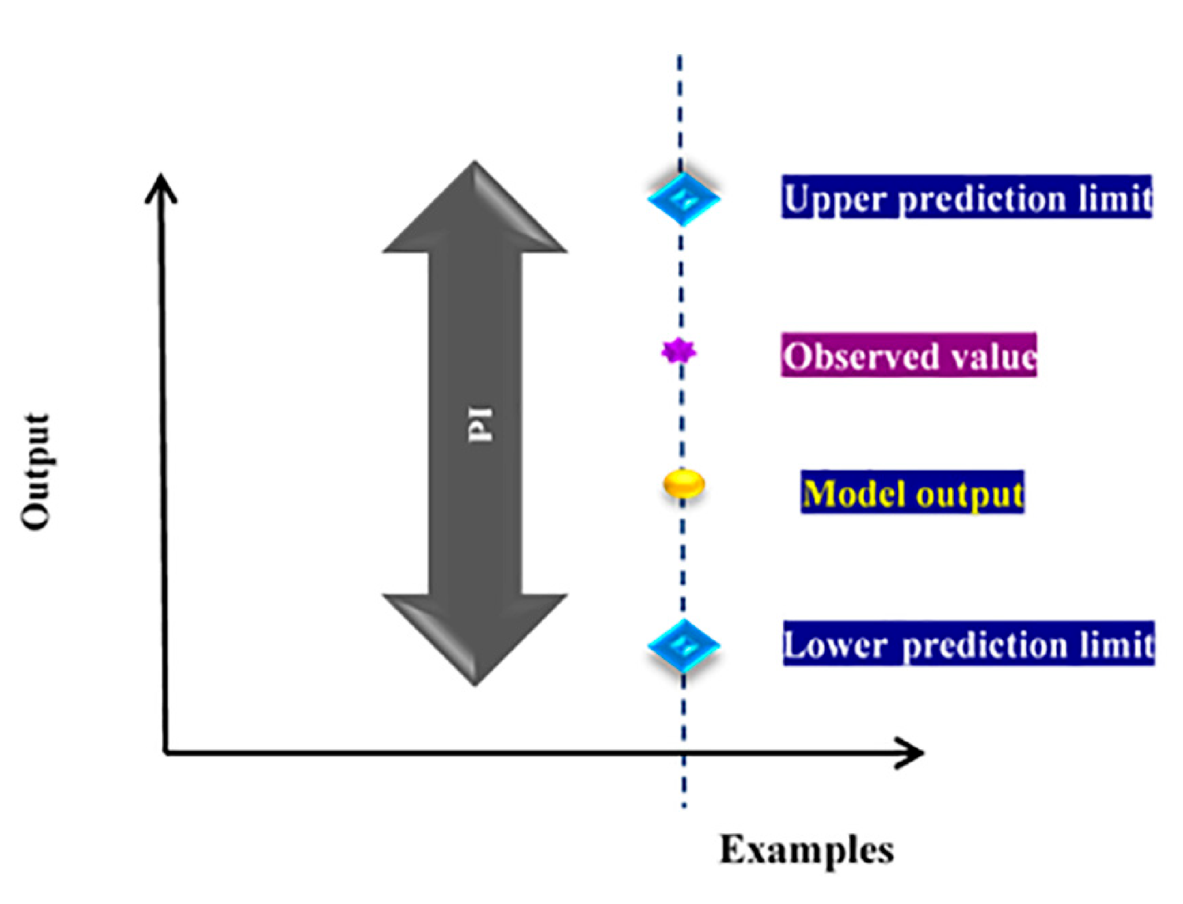
2. PIs Concepts
3. PIs Assessment Measures
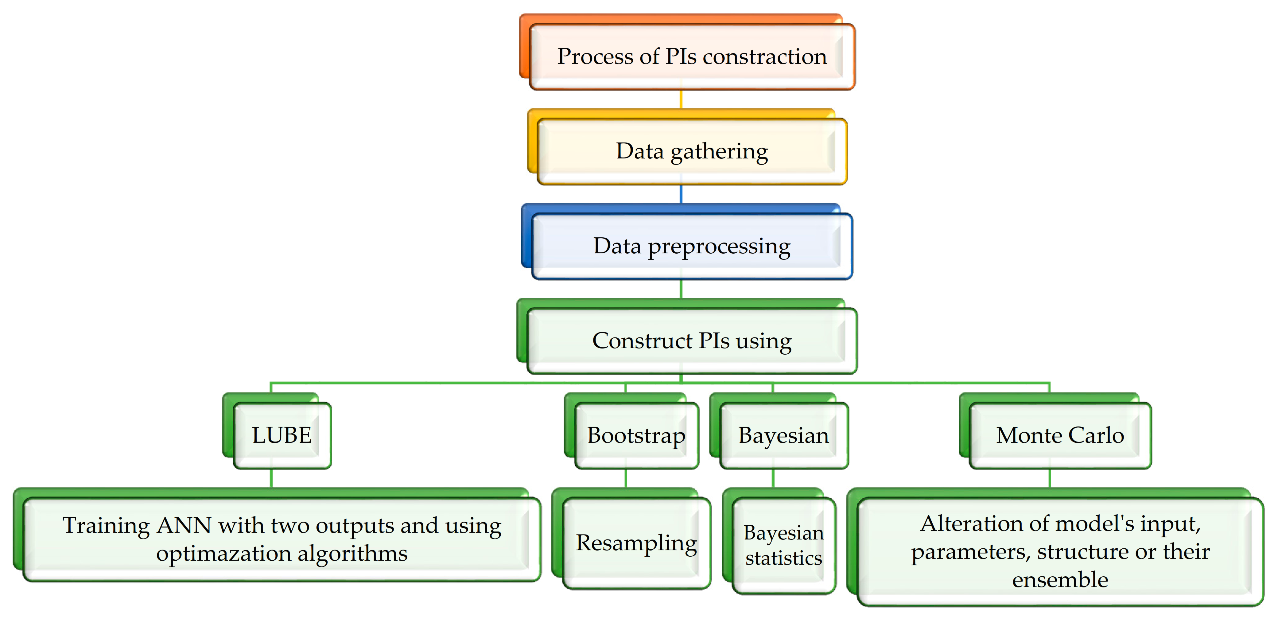
4. PIs Construction Methods
4.1. Bayesian Method
4.2. Monte Carlo Method
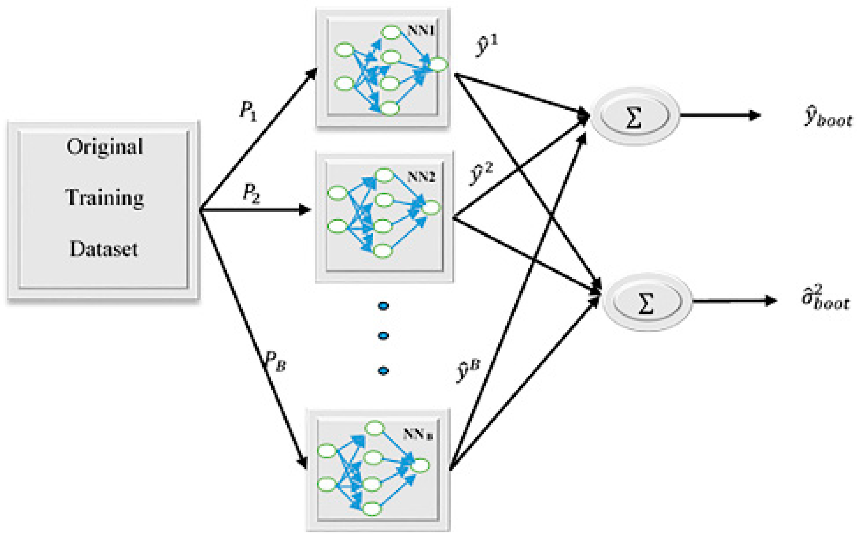
4.3. Bootstrap Method
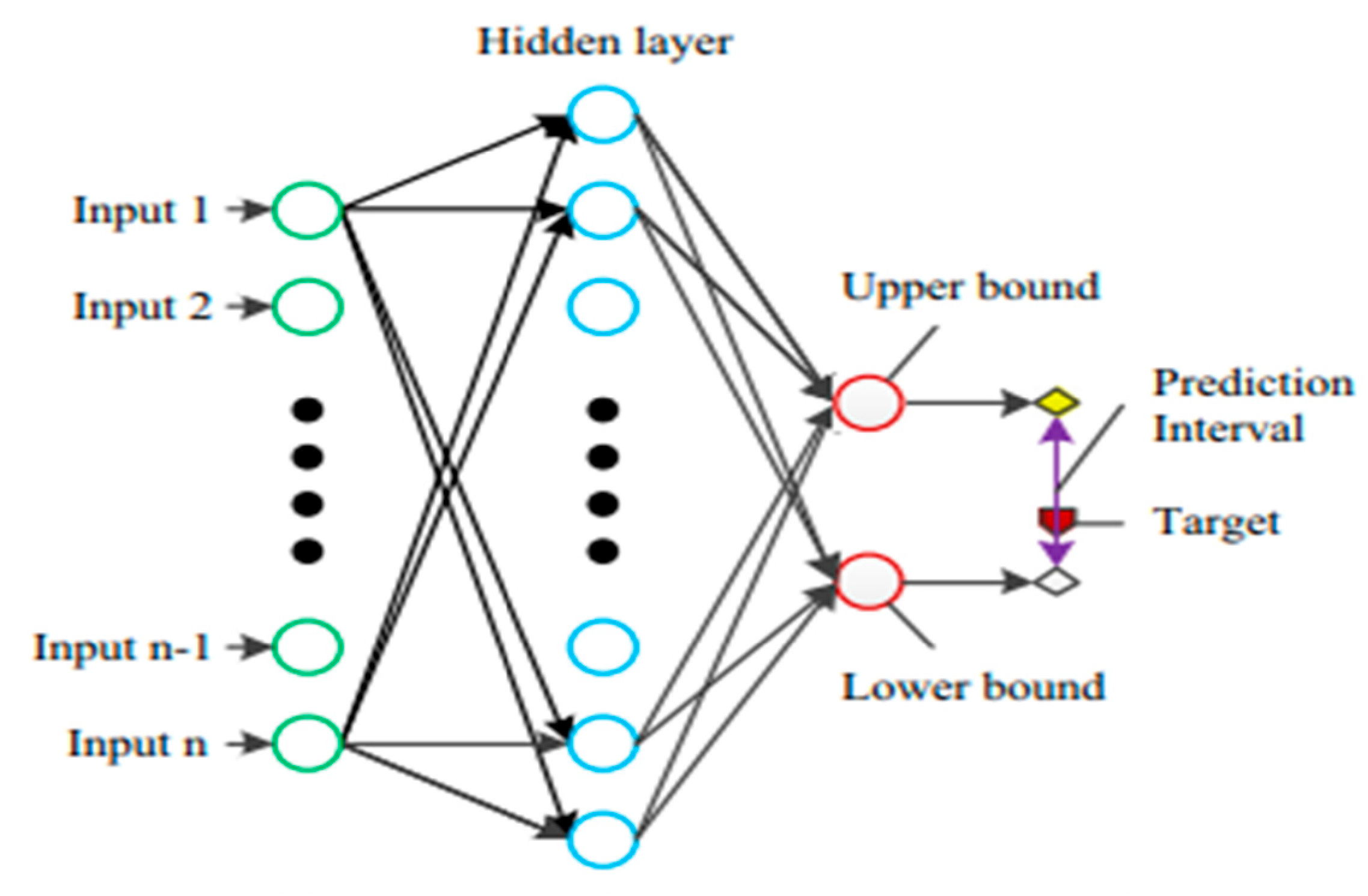
4.4. LUBE Method
5. Comparison of the PIs Construction Methods
6. Gaps and Suggestions for Future Studies
- i.
- Most of the PIs construction methods applied coverage and width criteria and their combination, but there is not any criterion in order to present information about the probability and reliability of the lower and upper bounds of the constructed PIs. Therefore, future studies may develop and present some criteria about this issue, for example, proximity of the target to the upper or lower bounds.
- ii.
- The reviewing of multiple studies showed that there is not any study that uses the delta method for PIs construction. Although it may have high level of computational cost, according to its reliable performance in other fields as expressed in Khosravi, Nahavandi, Creighton and Atiya [14], it is proposed that one apply this method in hydrological studies as well.
- iii.
- The performance of the LUBE method, as the most robust method of PI construction, can be improved in different aspects in order to obtain more reliable PIs. The implementation could be augmented by combining with the ANN structure selection techniques.
- iv.
- Adaptation between point prediction and PIs has not been examined, yet significantly presented. Therefore, it can be recommended that future works analyze the adaptation and correlation between point prediction and PIs construction. Moreover, some criteria can be defined to capture simultaneously.
- v.
- It is recommended that one apply the presented methods to assess the uncertainty associated with the improved version of the ANN, such as emotional ANN [72] and to investigate the effects of hormonal parameters in the reliability of the models.
- vi.
- The LUBE method performance is based on the cost functions. Some studies used multi-objective optimization cost function in which the coverage and width criteria were considered as cost function simultaneously. In contrast, some other studies used coverage and width combination criteria as the cost function, in which some parameters should be determined by trial and error. Therefore, future studies can compare the implementation of multi-objective and single-objective optimization methods. Moreover, future studies can propose the appropriate value of CWC parameters or propose a method for better and faster determination of the parameters’ values.
- vii.
- As there are few studies attempting to investigate other artificial intelligence methods such as ANFIS, it is recommended that one construct the PIs of those methods too.
7. Conclusions
Author Contributions
Funding
Institutional Review Board Statement
Informed Consent Statement
Data Availability Statement
Acknowledgments
Conflicts of Interest
References
- Loucks, D.P. Sustainable Water Resources Management. Water Int. 2000, 25, 3–10. [Google Scholar] [CrossRef]
- Nourani, V.; Kalantari, O. Integrated Artificial Neural Network for Spatiotemporal Modeling of Rainfall–Runoff–Sediment Processes. Environ. Eng. Sci. 2010, 27, 411–422. [Google Scholar] [CrossRef]
- Nourani, V.; Kisi, O.; Komasi, M. Two hybrid Artificial Intelligence approaches for modeling rainfall–runoff process. J. Hydrol. 2011, 402, 41–59. [Google Scholar] [CrossRef]
- Sharghi, E.; Nourani, V.; Najafi, H.; Molajou, A. Emotional ANN (EANN) and Wavelet-ANN (WANN) Approaches for Markovian and Seasonal Based Modeling of Rainfall-Runoff Process. Water Resour. Manag. 2018, 32, 3441–3456. [Google Scholar] [CrossRef]
- Sharifi, S.S.; Delirhasannia, R.; Nourani, V.; Sadraddini, A.A.; Ghorbani, A. Using artificial neural networks (ANNs) and adaptive neuro-fuzzy inference system (ANFIS) for modeling and sensitivity analysis of effective rainfall. Recent Adv. Contin. Mech. Hydrol. Ecol. 2013, 3, 133–139. [Google Scholar]
- Latifoglu, L. Evaluating Stream Flow Forecasting Performance Using Adaptive Network Based Fuzzy Logic Inference System, Artificial Neural Networks with Feature Selection. EPSTEM 2020, 11, 125–130. [Google Scholar]
- Klomjit, J.; Ngaopitakkul, A. Comparison of Artificial Intelligence Methods for Fault Classification of the 115-kV Hybrid Transmission System. Appl. Sci. 2020, 10, 3967. [Google Scholar] [CrossRef]
- Niu, W.-J.; Feng, Z.-K.; Feng, B.-F.; Xu, Y.-S.; Min, Y.-W. Parallel computing and swarm intelligence based artificial intelligence model for multi-step-ahead hydrological time series prediction. Sustain. Cities Soc. 2021, 66, 102686. [Google Scholar] [CrossRef]
- Nourani, V.; Komasi, M.; Mano, A. A Multivariate ANN-Wavelet Approach for Rainfall–Runoff Modeling. Water Resour. Manag. 2009, 23, 2877–2894. [Google Scholar] [CrossRef]
- Elshorbagy, A.; Corzo, G.; Srinivasulu, S.; Solomatine, D.P. Experimental investigation of the predictive capabilities of data driven modeling techniques in hydrology—Part 1: Concepts and methodology. Hydrol. Earth Syst. Sci. 2010, 14, 1931–1941. [Google Scholar] [CrossRef] [Green Version]
- Huang, F.; Huang, J.; Jiang, S.; Zhou, C.-B. Landslide displacement prediction based on multivariate chaotic model and extreme learning machine. Eng. Geol. 2017, 218, 173–186. [Google Scholar] [CrossRef]
- Refsgaard, J.C.; Van Der Sluijs, J.P.; Brown, J.; Van Der Keur, P. A framework for dealing with uncertainty due to model structure error. Adv. Water Resour. 2006, 29, 1586–1597. [Google Scholar] [CrossRef] [Green Version]
- Zio, E.; Aven, T. Uncertainties in smart grids behavior and modeling: What are the risks and vulnerabilities? How to analyze them? Energy Policy 2011, 39, 6308–6320. [Google Scholar] [CrossRef]
- Khosravi, A.; Nahavandi, S.; Creighton, D.; Atiya, A.F. Comprehensive Review of Neural Network-Based Prediction Intervals and New Advances. IEEE Trans. Neural Netw. 2011, 22, 1341–1356. [Google Scholar] [CrossRef]
- Quan, H.; Srinivasan, D.; Khosravi, A. Incorporating Wind Power Forecast Uncertainties into Stochastic Unit Commitment Using Neural Network-Based Prediction Intervals. IEEE Trans. Neural Netw. Learn. Syst. 2015, 26, 2123–2135. [Google Scholar] [CrossRef]
- Chatfield, C. Calculating interval forecasts. J. Bus. Econ. Stat. 1993, 11, 121–135. [Google Scholar]
- Ma, J.; Niu, X.; Tang, H.; Wang, Y.; Wen, T.; Zhang, J. Displacement Prediction of a Complex Landslide in the Three Gorges Reservoir Area (China) Using a Hybrid Computational Intelligence Approach. Complexity 2020, 2020, 1–15. [Google Scholar] [CrossRef]
- Shuai, Y.; Notton, G.; Duchaud, J.-L.; Almorox, J.; Yaseen, Z.M. Solar irradiation prediction intervals based on Box–Cox transformation and univariate representation of periodic autoregressive model. Renew. Energy Focus 2020, 33, 43–53. [Google Scholar] [CrossRef]
- Chryssolouris, G.; Lee, M.; Ramsey, A. Confidence interval prediction for neural network models. IEEE Trans. Neural Netw. 1996, 7, 229–232. [Google Scholar] [CrossRef]
- Momotaz, B.; Dohi, T. Prediction Interval of Cumulative Number of Software Faults Using Multilayer Perceptron. Flex. Gen. Uncertain. Optim. 2015, 619, 43–58. [Google Scholar] [CrossRef]
- Mackay, D.J.C. A Practical Bayesian Framework for Backpropagation Networks. Neural Comput. 1992, 4, 448–472. [Google Scholar] [CrossRef]
- Kasiviswanathan, K.S.; Sudheer, K. Methods used for quantifying the prediction uncertainty of artificial neural network based hydrologic models. Stoch. Environ. Res. Risk Assess. 2017, 31, 1659–1670. [Google Scholar] [CrossRef]
- Efron, B.; Tibshirani, R.J. An Introduction to the Bootstrap; CRC Press: Boca Raton, FL, USA, 1994. [Google Scholar]
- Lu, J.; Ding, J.; Dai, X.; Chai, T. Ensemble Stochastic Configuration Networks for Estimating Prediction Intervals: A Simultaneous Robust Training Algorithm and Its Application. IEEE Trans. Neural Netw. Learn. Syst. 2020, 31, 5426–5440. [Google Scholar] [CrossRef]
- Khosravi, A.; Nahavandi, S.; Creighton, D.; Atiya, A.F. Lower Upper Bound Estimation Method for Construction of Neural Network-Based Prediction Intervals. IEEE Trans. Neural Netw. 2010, 22, 337–346. [Google Scholar] [CrossRef]
- Cannon, A.J.; Whitfield, P.H. Downscaling recent streamflow conditions in British Columbia, Canada using ensemble neural network models. J. Hydrol. 2002, 259, 136–151. [Google Scholar] [CrossRef]
- Jeong, D.-I.; Kim, Y. Rainfall-runoff models using artificial neural networks for ensemble streamflow prediction. Hydrol. Process. 2005, 19, 3819–3835. [Google Scholar] [CrossRef]
- Fleming, S.W.; Bourdin, D.R.; Campbell, D.; Stull, R.B.; Gardner, T. Development and Operational Testing of a Super-Ensemble Artificial Intelligence Flood-Forecast Model for a Pacific Northwest River. JAWRA J. Am. Water Resour. Assoc. 2014, 51, 502–512. [Google Scholar] [CrossRef]
- Kan, G.; Yao, C.; Li, Q.; Li, Z.; Yu, Z.; Liu, C.; Ding, L.; He, X.; Liang, K. Improving event-based rainfall-runoff simulation using an ensemble artificial neural network based hybrid data-driven model. Stoch. Environ. Res. Risk Assess. 2015, 29, 1345–1370. [Google Scholar] [CrossRef]
- Kim, S.E.; Seo, I.W. Artificial Neural Network ensemble modeling with conjunctive data clustering for water quality prediction in rivers. HydroResearch 2015, 9, 325–339. [Google Scholar] [CrossRef]
- Kim, S.; Kim, H.S. Uncertainty Reduction of the Flood Stage Forecasting Using Neural Networks Model1. JAWRA J. Am. Water Resour. Assoc. 2008, 44, 148–165. [Google Scholar] [CrossRef]
- Yang, C.-C.; Chen, C.-S. Application of integrated back-propagation network and self organizing map for flood forecasting. Hydrol. Process. 2009, 23, 1313–1323. [Google Scholar] [CrossRef]
- Srivastav, R.; Sudheer, K.; Chaubey, I. A simplified approach to quantifying predictive and parametric uncertainty in artificial neural network hydrologic models. Water Resour. Res. 2007, 43. [Google Scholar] [CrossRef] [Green Version]
- Boucher, M.; Perreault, L.; Anctil, F. Tools for the assessment of hydrological ensemble forecasts obtained by neural networks. J. Hydroinform. 2009, 11, 297–307. [Google Scholar] [CrossRef] [Green Version]
- Sharma, S.K.; Tiwari, K. Bootstrap based artificial neural network (BANN) analysis for hierarchical prediction of monthly runoff in Upper Damodar Valley Catchment. J. Hydrol. 2009, 374, 209–222. [Google Scholar] [CrossRef]
- Kant, A.; Suman, P.K.; Giri, B.K.; Tiwari, M.K.; Chatterjee, C.; Nayak, P.C.; Kumar, S. Comparison of multi-objective evolutionary neural network, adaptive neuro-fuzzy inference system and bootstrap-based neural network for flood forecasting. Neural Comput. Appl. 2013, 23, 231–246. [Google Scholar] [CrossRef]
- Zhang, X.; Liang, F.; Srinivasan, R.; Van Liew, M. Estimating uncertainty of streamflow simulation using Bayesian neural networks. Water Resour. Res. 2009, 45. [Google Scholar] [CrossRef]
- Khan, M.S.; Coulibaly, P. Assessing Hydrologic Impact of Climate Change with Uncertainty Estimates: Bayesian Neural Network Approach. J. Hydrometeorol. 2010, 11, 482–495. [Google Scholar] [CrossRef]
- Zhang, X.; Liang, F.; Yu, B.; Zong, Z. Explicitly integrating parameter, input, and structure uncertainties into Bayesian Neural Networks for probabilistic hydrologic forecasting. J. Hydrol. 2011, 409, 696–709. [Google Scholar] [CrossRef]
- Zhang, X.; Zhao, K. Bayesian Neural Networks for Uncertainty Analysis of Hydrologic Modeling: A Comparison of Two Schemes. Water Resour. Manag. 2012, 26, 2365–2382. [Google Scholar] [CrossRef]
- Humphrey, G.B.; Gibbs, M.S.; Dandy, G.; Maier, H.R. A hybrid approach to monthly streamflow forecasting: Integrating hydrological model outputs into a Bayesian artificial neural network. J. Hydrol. 2016, 540, 623–640. [Google Scholar] [CrossRef]
- Shen, S.; Zeng, G.; Liang, J.; Li, X.; Tan, Y.; Li, Z.; Li, J. Markov Chain Monte Carlo Approach for Parameter Uncertainty Quantification and Its Impact on Groundwater Mass Transport Modeling: Influence of Prior Distribution. Environ. Eng. Sci. 2014, 31, 487–495. [Google Scholar] [CrossRef]
- Tongal, H.; Booij, M.J. Quantification of parametric uncertainty of ANN models with GLUE method for different streamflow dynamics. Stoch. Environ. Res. Risk Assess. 2017, 31, 993–1010. [Google Scholar] [CrossRef]
- Snyder, H. Literature review as a research methodology: An overview and guidelines. J. Bus. Res. 2019, 104, 333–339. [Google Scholar] [CrossRef]
- Torres-Carrión, P.V.; González-González, C.S.; Aciar, S.; Rodríguez-Morales, G. Methodology for Systematic Literature Review Applied to Engineering and Education. In Proceedings of the 2018 IEEE Global Engineering Education Conference (EDUCON), Tenerife, Spain, 17–20 April 2018; pp. 1364–1373. [Google Scholar]
- Shamseer, L.; Moher, D.; Clarke, M.; Ghersi, D.; Liberati, A.; Petticrew, M.; Shekelle, P.; Stewart, L.A. Preferred reporting items for systematic review and meta-analysis protocols (PRISMA-P) 2015: Elaboration and explanation. BMJ 2015, 349, 1–25. [Google Scholar] [CrossRef] [Green Version]
- Moher, D.; Shamseer, L.; Clarke, M.; Ghersi, D.; Liberati, A.; Petticrew, M.; Shekelle, P.; Stewart, L.A. Preferred reporting items for systematic review and meta-analysis protocols (PRISMA-P) 2015 statement. Syst. Rev. 2015, 4, 1. [Google Scholar] [CrossRef] [Green Version]
- Mengist, W.; Soromessa, T.; Legese, G. Method for conducting systematic literature review and meta-analysis for environmental science research. MethodsX 2020, 7, 100777. [Google Scholar] [CrossRef]
- Hasan, H.H.; Razali, S.F.M.; Muhammad, N.; Ahmad, A. Research Trends of Hydrological Drought: A Systematic Review. Water 2019, 11, 2252. [Google Scholar] [CrossRef] [Green Version]
- Harrison-Atlas, D.; Theobald, D.M.; Goldstein, J.H. A systematic review of approaches to quantify hydrologic ecosystem services to inform decision-making. Int. J. Biodivers. Sci. Ecosyst. Serv. Manag. 2016, 12, 160–171. [Google Scholar] [CrossRef] [Green Version]
- Kasiviswanathan, K.S.; Sudheer, K.P. Comparison of methods used for quantifying prediction interval in artificial neural network hydrologic models. Model. Earth Syst. Environ. 2016, 2, 1–11. [Google Scholar] [CrossRef]
- Talebizadeh, M.; Moridnejad, A. Uncertainty analysis for the forecast of lake level fluctuations using ensembles of ANN and ANFIS models. Expert Syst. Appl. 2011, 38, 4126–4135. [Google Scholar] [CrossRef]
- Kasiviswanathan, K.S.; Sudheer, K. Quantification of the predictive uncertainty of artificial neural network based river flow forecast models. Stoch. Environ. Res. Risk Assess. 2012, 27, 137–146. [Google Scholar] [CrossRef]
- Kumar, S.; Tiwari, M.K.; Chatterjee, C.; Mishra, A. Reservoir Inflow Forecasting Using Ensemble Models Based on Neural Networks, Wavelet Analysis and Bootstrap Method. Water Resour. Manag. 2015, 29, 4863–4883. [Google Scholar] [CrossRef]
- Wang, Y.; Zheng, T.; Zhao, Y.; Jiang, J.; Wang, Y.; Guo, L.; Wang, P. Monthly water quality forecasting and uncertainty assessment via bootstrapped wavelet neural networks under missing data for Harbin, China. Environ. Sci. Pollut. Res. 2013, 20, 8909–8923. [Google Scholar] [CrossRef]
- Kasiviswanathan, K.; He, J.; Sudheer, K.; Tay, J.-H. Potential application of wavelet neural network ensemble to forecast streamflow for flood management. J. Hydrol. 2016, 536, 161–173. [Google Scholar] [CrossRef]
- Nourani, V.; Paknezhad, N.J.; Sharghi, E.; Khosravi, A. Estimation of prediction interval in ANN-based multi-GCMs downscaling of hydro-climatologic parameters. J. Hydrol. 2019, 579, 124226. [Google Scholar] [CrossRef]
- Shrestha, D.L.; Kayastha, N.; Solomatine, D.P. A novel approach to parameter uncertainty analysis of hydrological models using neural networks. Hydrol. Earth Syst. Sci. 2009, 13, 1235–1248. [Google Scholar] [CrossRef] [Green Version]
- Seifi, A.; Ehteram, M.; Singh, V.P.; Mosavi, A. Modeling and Uncertainty Analysis of Groundwater Level Using Six Evolutionary Optimization Algorithms Hybridized with ANFIS, SVM, and ANN. Sustainability 2020, 12, 4023. [Google Scholar] [CrossRef]
- Tapoglou, E.; Varouchakis, E.A.; Trichakis, I.; Karatzas, G.P. Hydraulic head uncertainty estimations of a complex artificial intelligence model using multiple methodologies. J. Hydroinform. 2020, 22, 205–218. [Google Scholar] [CrossRef]
- Kasiviswanathan, K.; Cibin, R.; Sudheer, K.; Chaubey, I. Constructing prediction interval for artificial neural network rainfall runoff models based on ensemble simulations. J. Hydrol. 2013, 499, 275–288. [Google Scholar] [CrossRef]
- Taormina, R.; Chau, K.-W. ANN-based interval forecasting of streamflow discharges using the LUBE method and MOFIPS. Eng. Appl. Artif. Intell. 2015, 45, 429–440. [Google Scholar] [CrossRef]
- Zhang, H.; Zhou, J.; Ye, L.; Zeng, X.; Chen, Y. Lower Upper Bound Estimation Method Considering Symmetry for Construction of Prediction Intervals in Flood Forecasting. Water Resour. Manag. 2015, 29, 5505–5519. [Google Scholar] [CrossRef]
- Kasiviswanathan, K.; Sudheer, K.; He, J. Probabilistic and ensemble simulation approaches for input uncertainty quantification of artificial neural network hydrological models. Hydrol. Sci. J. 2018, 63, 101–113. [Google Scholar] [CrossRef]
- Nourani, V.; Sayyah-Fard, M.; Aalami, M.T.; Sharghi, E. Data pre-processing effect on ANN-based prediction intervals construction of the evaporation process at different climate regions in Iran. J. Hydrol. 2020, 588, 125078. [Google Scholar] [CrossRef]
- Chen, X.-Y.; Chau, K.-W. Uncertainty Analysis on Hybrid Double Feedforward Neural Network Model for Sediment Load Estimation with LUBE Method. Water Resour. Manag. 2019, 33, 3563–3577. [Google Scholar] [CrossRef]
- Kasiviswanathan, K.S.; Sudheer, K.P.; Soundharajan, B.-S.; Adeloye, A.J. Implications of uncertainty in inflow forecasting on reservoir operation for irrigation. Paddy Water Environ. 2020, 1–13. [Google Scholar] [CrossRef]
- Shrestha, D.L.; Solomatine, D.P. Machine learning approaches for estimation of prediction interval for the model output. Neural Netw. 2006, 19, 225–235. [Google Scholar] [CrossRef]
- Shrivastava, N.A.; Khosravi, A.; Panigrahi, B. Prediction Interval Estimation of Electricity Prices Using PSO-Tuned Support Vector Machines. IEEE Trans. Ind. Inform. 2015, 11, 322–331. [Google Scholar] [CrossRef]
- Grant, E.L.; Leavenworth, R.S. Statistical Quality and Control; McGraw-Hill: New York, NY, USA, 1972. [Google Scholar]
- Quan, H.; Srinivasan, D.; Khosravi, A. Particle swarm optimization for construction of neural network-based prediction intervals. Neurocomputing 2014, 127, 172–180. [Google Scholar] [CrossRef]
- Nourani, V. An Emotional ANN (EANN) approach to modeling rainfall-runoff process. J. Hydrol. 2017, 544, 267–277. [Google Scholar] [CrossRef]


| Method | Author | Name of the Journal |
|---|---|---|
| Ensemble ANN | Cannon and Whitfield [26] | Journal of Hydrology |
| Jeong and Kim [27] | Hydrological Processes | |
| Fleming, Bourdin, Campbell, Stull and Gardner [28] | Water Resources Research | |
| Kan, Yao, Li, Li, Yu, Liu, Ding, He and Liang [29] | Stochastic Environment Research and Risk Assessment | |
| Kim and Seo [30] | Journal of Hydro-environment Research | |
| Sensitivity analysis | Kim and Kim [31] | The Journal of the American Water Resources Association |
| Self-organizing map | Yang and Chen [32] | Hydrological Processes |
| Bootstrap | Srivastav, Sudheer and Chaubey [33] | Water Resources Research |
| Boucher, Perreault and Anctil [34] | Hydrology and Earth System Sciences | |
| Sharma and Tiwari [35] | Journal of Hydrology | |
| Kant, Suman, Giri, Tiwari, Chatterjee, Nayak and Kumar [36] | Neural Computing and Applications | |
| Bayesian | Zhang, Liang, Srinivasan and Van Liew [37] | Water Resources Research |
| Khan and Coulibaly [38] | Journal of Hydrometeorology | |
| Zhang, Liang, Yu and Zong [39] | Journal of Hydrology | |
| Zhang and Zhao [40] | Journal of Hydrology | |
| Humphrey, Gibbs, Dandy and Maier [41] | Journal of Hydrology | |
| Markov Chain Monte Carlo | Shen, Zeng, Liang, Li, Tan, Li and Li [42] | Water Resources Research |
| GLUBE | Tongal and Booij [43] | Stochastic Environmental Research and Risk Assessment |
| Keywords | Number of Cites | Author | PI Construction Method | Number of Papers |
|---|---|---|---|---|
| ANN; Bayesian; Bootstrap; PI; Uncertainty | 27 | Kasiviswanathan and Sudheer [51] | Bayesian | 1 |
| Uncertainty analysis; PIs;Lake level; ANN; ANFIS; Bootstrapping | 129 | Talebizadeh and Moridnejad [52] | Bootstrap | 7 |
| ANN; Bootstrap technique; Hydrological processes; Non-linear function; Taylor series | 72 | Kasiviswanathan and Sudheer [53] | ||
| Uncertainty; Flood forecasting; Bootstrap; ANNs; Ensemble | 60 | Kumar, Tiwari, Chatterjee and Mishra [54] | ||
| Water quality forecasting; Wavelet neural network; Bootstrap; Uncertainty; Data missing; Data filling; Songhua River | 33 | Wang, Zheng, Zhao, Jiang, Wang, Guo and Wang [55] | ||
| ANN; Bayesian; Bootstrap; PI; Uncertainty | 27 | Kasiviswanathan and Sudheer [51] | ||
| ANNs; ensemble simulation; input uncertainty; prediction uncertainty; rainfall–runoff modeling | 82 | Kasiviswanathan, He, Sudheer and Tay [56] | ||
| General circulation models;Downscaling; PIs; ANN | 9 | Nourani, Paknezhad, Sharghi and Khosravi [57] | ||
| 111 | Shrestha, Kayastha and Solomatine [58] | Monte Carlo | 3 | |
| groundwater; artificial intelligence; hydrologic model; groundwater level prediction; machine learning;artificial neural network | 7 | Seifi, Ehteram, Singh and Mosavi [59] | ||
| ANNs; Bayesian uncertainty; fuzzy logic; kriging; uncertainty analysis | 5 | Tapoglou, Varouchakis, Trichakis and Karatzas [60] | ||
| Ensemble Optimization; PI;Rainfall runoff models | 68 | Kasiviswanathan, Cibin, Sudheer and Chaubey [61] | LUBE | 9 |
| MOFIPS; PSO; Prediction interval; LUBE; Neural networks; Streamflow prediction | 63 | Taormina and Chau [62] | ||
| PI; Symmetry; ANN; Uncertainty; Flood forecasting; Shuffled complex evolution | 16 | Zhang, Zhou, Ye, Zeng and Chen [63] | ||
| ANN; Bayesian; Bootstrap; PI; Uncertainty | 27 | Kasiviswanathan and Sudheer [51] | ||
| ANN; ensemble simulation; input uncertainty; prediction uncertainty; rainfall–runoff modeling | 8 | Kasiviswanathan, Sudheer and He [64] | ||
| General circulation models; DownscalingPI; ANN | 9 | Nourani, Paknezhad, Sharghi and Khosravi [57] | ||
| Evaporation; Neural network; Prediction interval; Uncertainty quantifying; Wavelet de-noising; Jitterd data | 1 | Nourani, Sayyah-Fard, Alami and Sharghi [65] | ||
| Uncertainty analysis; Hybrid double feedforward neural network; Sediment load estimation; Lower upper bound estimation | 27 | Chen and Chau [66] | ||
| ANN; Crop simulation; Reservoir operation; Optimization; Uncertainty | 0 | Kasiviswanathan, Sudheer, Soundharajan and Adeloye [67] |
| PI | z |
|---|---|
| 75% | 1.15 |
| 90% | 1.64 |
| 95% | 1.96 |
| 99% | 2.58 |
| Method | Run Time | Number of Required Networks | Computational Burden | Reliability | Reference | |
|---|---|---|---|---|---|---|
| Bayesian |  Conceptual representation of the Bayesian model for inference of parameters. Conceptual representation of the Bayesian model for inference of parameters. | high | One | high | high | [21] |
| Monte Carlo |  General overview of the Monte Carlo algorithm. General overview of the Monte Carlo algorithm. | high | More than 1 | medium | medium | [58] |
| Bootstrap |  Schematic of the bootstrap method, PB stands for training data sub-sets. Schematic of the bootstrap method, PB stands for training data sub-sets. | high | More than 1 | low | medium | [14] |
| LUBE |  The structure of the ANN in the LUBE method The structure of the ANN in the LUBE method | low | One | low | high | [24] |
Publisher’s Note: MDPI stays neutral with regard to jurisdictional claims in published maps and institutional affiliations. |
© 2021 by the authors. Licensee MDPI, Basel, Switzerland. This article is an open access article distributed under the terms and conditions of the Creative Commons Attribution (CC BY) license (http://creativecommons.org/licenses/by/4.0/).
Share and Cite
Nourani, V.; Paknezhad, N.J.; Tanaka, H. Prediction Interval Estimation Methods for Artificial Neural Network (ANN)-Based Modeling of the Hydro-Climatic Processes, a Review. Sustainability 2021, 13, 1633. https://doi.org/10.3390/su13041633
Nourani V, Paknezhad NJ, Tanaka H. Prediction Interval Estimation Methods for Artificial Neural Network (ANN)-Based Modeling of the Hydro-Climatic Processes, a Review. Sustainability. 2021; 13(4):1633. https://doi.org/10.3390/su13041633
Chicago/Turabian StyleNourani, Vahid, Nardin Jabbarian Paknezhad, and Hitoshi Tanaka. 2021. "Prediction Interval Estimation Methods for Artificial Neural Network (ANN)-Based Modeling of the Hydro-Climatic Processes, a Review" Sustainability 13, no. 4: 1633. https://doi.org/10.3390/su13041633