Bayesian Model Averaging: A Unique Model Enhancing Forecasting Accuracy for Daily Streamflow Based on Different Antecedent Time Series

Abstract

Streamflow forecasting is a vital task for hydrology and water resources engineering, and the different artificial intelligence (AI) approaches have been employed for this purposes until now. Additionally, the forecasting accuracy and uncertainty estimation are the meaningful assignments that need to be recognized. The addressed research investigates the potential of novel ensemble approach, Bayesian model averaging (BMA), in streamflow forecasting using daily time series data from two stations (i.e., Hongcheon and Jucheon), South Korea. Six categories (i.e., M1–M6) of input combination using different antecedent times were employed for streamflow forecasting. The outcomes of BMA model were compared with those of multivariate adaptive regression spline (MARS), M5 model tree (M5Tree), and Kernel extreme learning machines (KELM) models considering four assessment indexes, root mean square error (RMSE), Nash-Sutcliffe efficiency (NSE), correlation coefficient (R), and mean absolute error (MAE). The results revealed the superior accuracy of BMA model over three machine learning models in daily streamflow forecasting. Considering RMSE values among the best models during testing phase, the best BMA model (i.e., BMA2) enhanced the forecasting accuracy of MARS1, M5Tree4, and KELM3 models by 5.2%, 5.8%, and 3.4% in Hongcheon station. Additionally, the best BMA model (i.e., BMA1) improved the forecasting accuracy of MARS1, M5Tree1, and KELM1 models by 6.7%, 9.5%, and 3.7% in Jucheon station. In addition, the best BMA models in both stations allowed the uncertainty estimation, and produced higher uncertainty of peak flows compared to that of low flows. As one of the most robust and effective tools, therefore, the BMA model can be successfully employed for streamflow forecasting with different antecedent times.

1. Introduction

Implementing a stable model to forecast streamflow can be influential for the fields of hydrology and water resources researches [1,2,3,4]. Streamflow forecasting, however, is an intricate project because of nonstationary time series and reliance on temporal and spatial parameters which have unclear and complicated components [5,6,7]. Increasing issue complications often depend on long antecedent times (or lead times) such as days and months [8,9,10,11]. Therefore, streamflow forecasting using different antecedent times can be categorized as universal assignment for hydrology and water resources researches [12,13,14,15,16].

Machine learning (ML) models have popular and flexible approaches for simulating and catching the nonlinear phenomena for science and engineering during three decades including multivariate adaptive regression spline (MARS), M5 model tree (M5Tree), and Kernel extreme learning model (KELM), etc. The MARS model has been successfully applied and employed for solving streamflow forecasting problems until now. Al-Sudani et al. [17] surveyed the ability of MARS incorporated with differential evolution (MARS-DE) model to forecast streamflow in Tigris River, Iraq. They investigated that the MARS-DE model provided a reliable forecasted accuracy for semi-arid streamflow. Adamowski et al. [18] managed the MARS model to forecast streamflow in Himalayan watershed, Uttaranchal State, India. They found that the MARS model preformed a superior forecasted accuracy compared to the artificial neural network (ANN) model. Tyralis et al. [19] utilized the MARS model for daily streamflow forecasting in 511 basins, USA. The MARS model, however, did not improve the performance of linear regression model obviously compared to the other models (e.g., extremely randomized trees, XGBoost, and polyMARS).

M5Tree model has also been utilized for perceiving the pros and cons of streamflow forecasting. Solomatine and Xue [20] applied the M5Tree model for flood forecasting in the Huai River, China. They provided that the forecasted accuracy of M5Tree model were similar with that of ANN models, and the hybrid model covering M5Tree and ANN indicated the best forecasted accuracy. Štravs and Brilly [21] developed the M5Tree model for low streamflow forecasting in the Sava River basin, Slovenia. They employed the recession streamflow data based on 7-day lead time for forecasting and showed the reliable accuracy. Sattari et al. [22] hired the M5Tree model for daily streamflow forecasting in the Sohu River, Turkey. They demonstrated that the M5Tree model forecasted 7-day lead time streamflow accurately. Adnan et al. [23] worked using the M5Tree model for monthly and daily streamflow forecasting in the Hunza River, Pakistan. This experiment said that the M5Tree model could not forecast monthly and daily streamflow effectively compared to the least square support vector machine (LSSVM) model.

However, the diverse researches using multiple machine learning models can be found for streamflow forecasting including the MARS and M5Tree models from the published articles and reports. Yaseen et al. [24] evaluated the MARS and M5Tree models for monthly streamflow forecasting in Turkey and Iraq. This document explained that the LSSVM model, however, forecasted the monthly streamflow accurately compared to the MARS and M5Tree models. Yin et al. [25] utilized the MARS and M5Tree models for streamflow forecasting in a semiarid and mountainous region, Northwestern China. They evaluated that the performance of M5Tree model was superior to the support vector regression (SVR) and MARS models for 1-, 2-, and 3-day lead times forecasting. Kisi et al. [26] investigated the MARS and M5Tree models for streamflow forecasting in the Mediterranean region, Turkey. This article showed that the MARS and M5Tree model did not accomplish the outstanding performance compared to the LSSVM model. Rezaie-Balf et al. [27] handled the MARS and M5Tree models to forecast daily streamflow in Iran and South Korea. They indicated that the MARS model combined ensemble empirical mode decomposition (EEMD) was the effective method to forecast streamflow based on 1-, 2-, 3-, and 4-day lead times. Additionally, Rezaie-Balf et al. [28] explored the MARS and M5Tree models to forecast the reservoir inflow for Aswan High Dam, Egypt. They discovered that the MARS model embedded with complete ensemble empirical mode decomposition with adaptive noise (CEEMDAN) suggested the reliable accuracy to forecast dam inflow up to 6-month lead time.

Extreme learning machines (ELM) has also been accomplished to understand the nonlinear behavior of streamflow forecasting. Lima et al. [29] forecasted the daily streamflow using the ELM model in British Columbia, Canada. This research explained that the online sequential extreme learning machine (OSELM) model was trained utilizing abundant dataset to choose the optimal parameters, and generated the effective performance to forecast streamflow based on 1-, 2-, and 3-day lead times. Yadav et al. [30] verified the ELM model for streamflow forecasting in the Neckar River, Germany. They illustrated that the OSELM model forecasted streamflow up to 6 h lead time accurately compared to the ANN, support vector machine (SVM), and genetic programming. Yaseen et al. [2] investigated the ELM model for forecasting monthly streamflow in the Tigris River, Iraq. They concluded that the ELM model surpassed the SVR and the generalized regression neural network (GRNN) models to forecast the monthly streamflow. Rezaie-Balf and Kisi [13] applied the ELM model for daily streamflow forecasting in the Tajan River, Iran. This study revealed that the evolutionary polynomial regression (EPR) model outperformed the multilayer perceptron neural network (MLPNN) and optimally pruned extreme learning machine (OPELM) models to forecast daily streamflow. Niu et al. [31] developed the ELM model for forecasting daily streamflow in Xinfengjiang Reservoir, China. They demonstrated that the ELM integrated with quantum particle swarm optimization (ELM-QPSO) model enhanced the performance accuracy of ELM model to forecast daily streamflow. Under addressed research, Kernel extreme learning machine (KELM), a special type of ELM model, has been considered.

BMA model is a unique approach to implement a mechanism and clarify the model uncertainty [32]. However, the limited researchers have developed and applied the BMA model for fields of hydrology and water resources engineering including streamflow, rainfall, and water stage, etc. Duan et al. [33] employed the BMA model to develop the stable hydrologic predictions. They surveyed that the BMA model carried out the effective probabilistic prediction compared to the original ensemble model. Jiang et al. [34] investigated the BMA model for evaluating the multi-satellite precipitation using simulated hydrological streamflows, South China. This research showed that the satellite streamflow was merged by the BMA model, and the simulated streamflow was improved effectively. Wang et al. [35] developed the BMA model for rainfall forecasting based on seasonal concept, Australia. They inspected that the BMA model outperformed the specific model with two fixed predictors to forecast the merging seasonal rainfall. Rathinasamy et al. [36] developed the BMA model for forecasting streamflow at different time-scales (i.e., daily, weekly, and monthly) in two stations, USA. They produced several wavelet Volterra to obtain ensemble BMA model. The BMA model coupling ensemble multi wavelet Volterra outperformed the single wavelet Volterra and the mean averaged ensemble wavelet Volterra clearly to forecast daily, weekly, and monthly streamflow. Liu and Merwade [37] developed the BMA model to operate the system of water stage prediction in the Black River watershed, Missouri and Arkansas, USA. They reported that the BMA model provided the accurate prediction for flood water stage. In addition, flood inundation range estimated from BMA flood map was more effective than the probabilistic flood inundation range.

It can be considered from literature reviews of the BMA model that there have been no previously published the articles using the BMA model to compare the performance accuracy of MARS, M5Tree, and KELM models for streamflow forecasting until now. The purposes of this article can be arranged as follows: (1) to evaluate various input category of streamflow data with different antecedent times, (2) to compare and assess the performance accuracy of multivariate adaptive regression spline (MARS), M5 model tree (M5Tree), Kernel extreme learning model (KELM), and Bayesian model averaging (BMA) models for streamflow forecasting, and (3) to map the uncertainty ranges utilizing the performance of novel BMA model.

2. Methodology

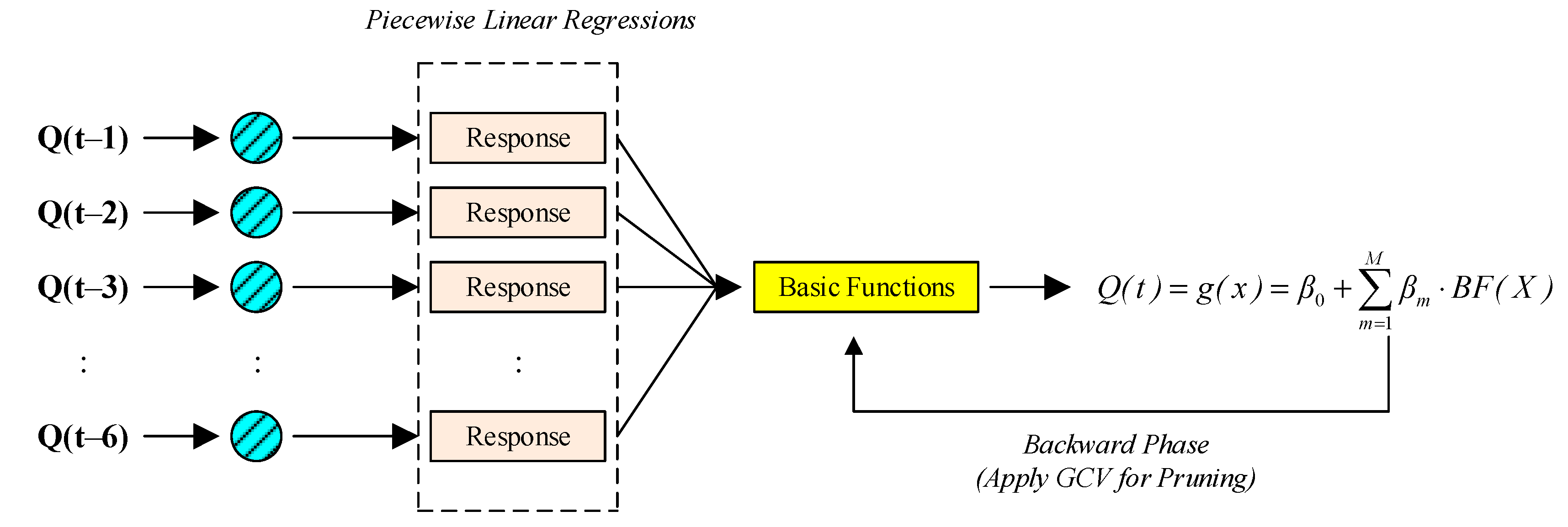
2.1. Multivariate Adaptive Regression Spline (MARS)

MARS model (see Figure 1) does not require the particular presumptions of practical relationships between input and output indicators [38]. The performance of MARS model using spline functions gives larger flexibility than linear ones based on curvature and thresholds. The basic functions (BFs), which are assigned as smooth polynomials (e.g., splines), are built using two step approaches. In the first approach, the model performance is enhanced until probabilistic nodes are identified. The second includes the elimination of lowest real terms. Imagine $y$ is an output indicator and $X=\left(X_1,\dots ,X_p\right)$ is an input indicator. Therefore, the actual response can be expressed using following Equation (1) [27,39].

$$y =f\left(X_1,\dots ,X_p\right)+e=f\left(x\right)+e$$

(1)

where $e$ = the error distribution. The MARS model achieves the approximate function (ƒ) using the BFs. The Equation (2) provides a linear combination of BFs and shared relation for the MARS model.

$$f\left(x\right)={\beta }_0+{\displaystyle \sum }_{m=1}^M{\beta }_m{\lambda }_m\left(x\right)$$

(2)

where individual ${\lambda }_m(x)$ = a spline function or output of two (or more) spline functions. The least squares method (LSM) can evaluate the coefficients ${\beta }_0$ (i.e., constant value). A model, therefore, can form the training error (e.g., having maximum reduction) using separating ${\beta }_0$ and basis pair. The following pair is boosted to the addressed model based on the $M$ BFs as [27,39]:

$${\hat{\beta }}_{M+1}{\lambda }_1\left(X\right)max\left(0,X_j-t\right)+{\hat{\beta }}_{M+2}{\lambda }_1\left(X\right)max\left(0,t-X_j\right)$$

(3)

where LSM can be applied for estimating $\beta$. When a novel BF is boosted to the model space, the associated interactions are recognized among the BFs. BFs are accumulated to the model for acquiring the maximum number of terms that deliver a sufficient fitness model. Then, a backward technique is applied to reduce the numbers of terms effectively. In the backward technique, BFs with the lowest accuracy are deleted to determine the best alternate model. Generalized cross validation (GCV), a method for comparing alternative models, can be represented as [27,39].

$$GCV=\frac{MSE}{{\left[1- \frac{N+dN}{M}\right]}^2}$$

(4)

where M and N = the number of observations and BFs, respectively, MSE = mean squared error, and d = the penalty of each BF. To broaden the knowledge of MARS model, [27] provided the detailed theory and application using MARS models for streamflow forecasting.

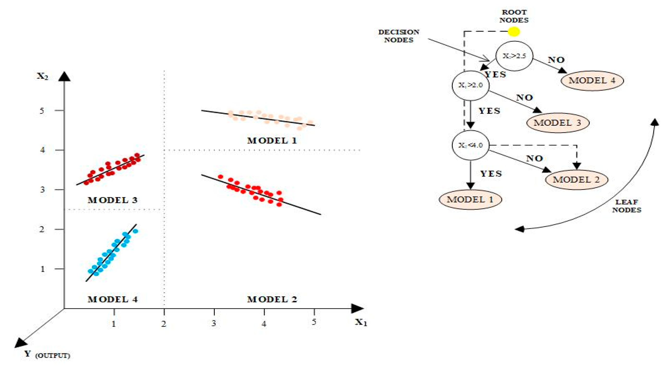
2.2. M5 Model Tree (M5Tree)

M5Tree model (see Figure 2) is a layered algorithm to judge the connection between input and output indicators [27,40]. The classification and regression trees (CART) is the basic algorithm for developing M5Tree model [41]. The M5Tree model assembles a linear-based model to the specific division which calculates the class properties of data portion leading to the leaf [27]. The standard deviation reduction (SDR) can influence to build the tree of M5Tree model. Additionally, it can reinforce the expected error reduction for specific points using Equation (5).

$$SDR=sd(E)-{\displaystyle \sum _i\frac{\left|E_i\right|}{\left|E\right|}}sd(E_i)$$

(5)

where E = a group of demonstrations that reach the leaf and E_i = a sub-group of input data to antecedent leaf. The pruning method was employed to suppress the overfitting burden and attain the accurate formation [27]. To apply the M5Tree model for streamflow forecasting, the previous articles (e.g., [20,27]) furnished the core approach to solve the addressed problems of streamflow forecasting.

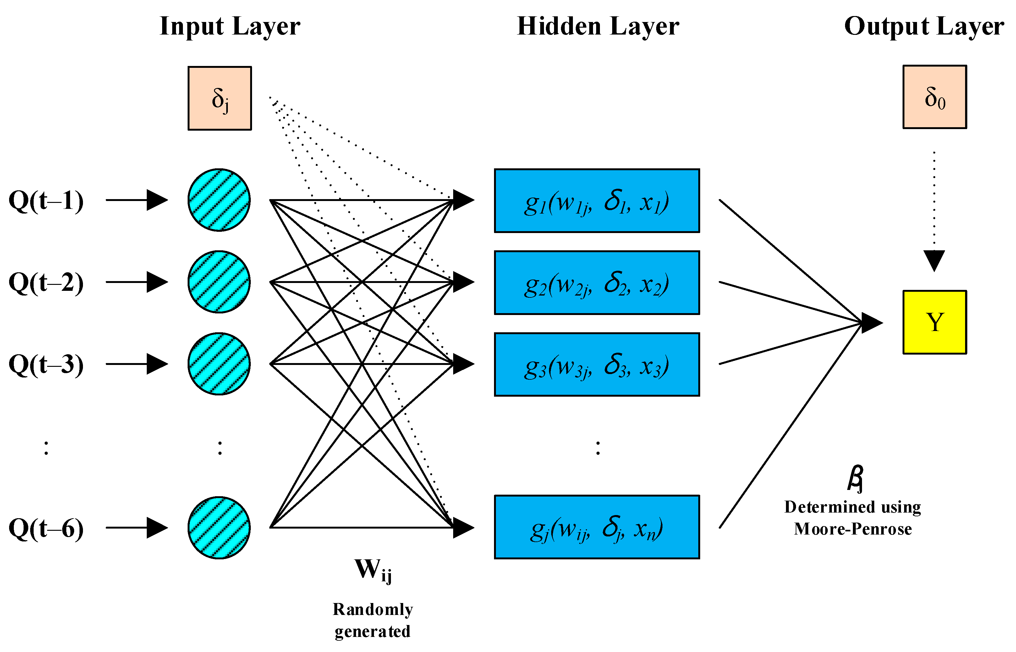
2.3. Kernel Extreme Learning Machines (KELM)

ELM model (see Figure 3), one of novel training algorithms for feedforward neural networks (FFNN) with single hidden layer, was recommended by the previous article of Huang et al. [42] to lessen the handicaps of conventional training algorithm and enhance the model accuracy [43,44]. The training speed of ELM model, which generates the connection weights randomly in the hidden layer, is faster than that of other models. Additionally, the performance of ELM model shows robust generalizations with accurate control [42]. The aforementioned specification evaluates the ELM model as a superior model compared to other models with conventional training algorithm. The conventional version of the ELM model meets the disadvantages of providing diverse accuracies in various trials because of randomly assigned connection weights. To solve the weak point of standard ELM model, Huang et al. [45] supplied the Kernel ELM (i.e., KELM) model by improving the process of allocating random connection weights between the input and hidden layers, which explains briefly the theory of KELM model. Detailed demonstration can be found in published article of Huang et al. [45]. The conventional FFNN model (i.e., having single hidden layer) with N hidden nodes can be shown using Equation (6).

$${\displaystyle \sum _{i=1}^N{\beta }_{i}g(W_i{x}_i+b_i}{)=y}_k, k=1,2,\dots ,M$$

(6)

where $g(\cdot )$, $b_i$, $W_i$, and ${\beta }_i$ = transfer function, specified bias randomly, connection weights from hidden to output layer, and connection weights from hidden and output layer, respectively. Equation (6), therefore, can be re-written as [43].

$$H\beta =Y$$

(7)

where $Y$ = N target values and $H$ = the matrix of hidden layer.

$$H={\left[\begin{array}{ccc}g(W_1\cdot x_1+b_1)& \cdots & g(W_M\cdot x_1+b_M)\\ ⋮& \ddots & ⋮\\ g(W_1\cdot x_N+b_1)& \cdots & g(W_M\cdot x_N+b_M)\end{array}\right]}_{N\times M}$$

(8)

where M = the number of nodes in the hidden layer. The connection weights in the output layer can be generated applying the Moore-Penrose generalized inverse (H⁺) of hidden layer matrix.

$$\beta =H^{+}Y$$

(9)

As one of accurate nonlinear regression models, the ELM model has been employed widely in the fields of hydrology and water resources engineering (e.g., [13,46]). In this study, 12 neurons and polynomial kernel were applied in hidden layer by applying trial and error process. Additionally, the regularization coefficient of KELM model was set to 10 to minimize difference between observed and forecasted streamflow values in both stations.

2.4. Bayesian Model Averaging (BMA)

BMA model, as a Bayesian inference, is implemented for model selection, forecasting, prediction, and estimation, and is also developed to combine the interferences and predictions from statistical models [32]. It can provide a criteria for simple model selection with limited simulations. One can simulate the parameter uncertainty utilizing a prior distribution as well as posterior parameter when requesting BMA model. This approach causes the brash inferences by neglecting uncertainty of candidate models [47]. This unique characteristics can provide a way to forecast natural behavior utilizing statistical post-processing approach [48,49,50]. Dismissing process, therefore, to acquire the posterior densities on BMA model parameters can be found from predictive probability density function (PDF) of x.

$$p(x|f_1,f_2,\dots ,f_M,{\theta }_1,{\theta }_2,\dots ,{\theta }_M)={\displaystyle \sum _{k=1}^M{\omega }_k{g}_k(x|f_k{\theta }_k)}$$

(10)

where $f_1,f_2,\dots ,f_M$ = the group for candidate models of a specific quantity x based on temporal and spatial scale, ${\theta }_k$ = estimated parameter, and ${\omega }_k$ = connection weights for the relative performance of every ensemble member ($f_k$). Therefore, the connection weights form the probability density and ${\displaystyle \sum _{k=1}^M{\omega }_k}=1$ [51]. In BMA model’ category, $f_k$ demonstrates a component PDF ($g_k(x|f_k{\theta }_k)$) [52].

2.5. Assessment of Models Performance

To figure out the performance of MARS, M5Tree, KELM, and BMA models, four assessment indexes were handled.

2.5.1. Root Mean Square Error (RMSE)

The error discrepancy between observed and forecasted streamflow values can be assessed by root mean square error (RMSE) function [53]. Perfect forecasting can be judged by RMSE = 0. In case of the highest error caused by the peak and higher values, RMSE can be distorted [54] and exploited for model evaluation with absolute units [55].

2.5.2. Nash-Sutcliffe Efficiency (NSE)

Evaluating the models’ capability can be accomplished by the Nash-Sutcliffe efficiency (NSE) function [56]. NSE = 0 when the squared difference between observed and forecasted streamflow values is immense to approve the variance in observed streamflow values. If NSE < 0, this indicates that the observed mean is better than forecasted one by the model [57]. If NSE = 1, all points are ideal category [58].

2.5.3. Correlation Coefficient (R)

The correlation coefficient (R) is defined as the ratio of dependent indicator from the independent one. If R = 0, it implies that streamflow cannot be forecasted using developed models, whereas if R = 1, it demonstrates that the observed and forecasted streamflows have a strong correlation.

2.5.4. Mean Absolute Error (MAE)

The mean absolute error (MAE) can supply better knowledge for a model’s forecasting, and cannot be contemplated in the vicinity of higher or lower significance. However, it assesses all derivations from observed streamflow values in the same manner [59]. If MAE = 0, it defines that the employed models can forecast streamflow absolutely, while if MAE = 1, it describes that the observed and forecasted streamflows do not have any relationship for forecasting category.

Four assessment indexes (i.e., RMSE, NSE, R, and MAE) can be implemented as Equations (11)–(14), respectively.

$$RMSE=\sqrt{\frac{1}{n}{\displaystyle \sum _{i=1}^n{[S_{obs}-S_{for}]}^2}}$$

(11)

$$NSE=1-\frac{{\displaystyle \sum _{i=1}^n{[S_{obs}-S_{for}]}^2}}{{\displaystyle \sum _{i=1}^n{[S_{obs}-{\overline{S}}_{for}]}^2}}$$

(12)

$$R=\frac{{\displaystyle \sum _{i=1}^n(S_{obs}-{\overline{S}}_{obs})(S_{for}-{\overline{S}}_{for})}}{\sqrt{{\displaystyle \sum _{i=1}^n{(S_{obs}-{\overline{S}}_{obs})}^2{\displaystyle \sum _{i=1}^n{(S_{for}-{\overline{S}}_{for})}^2}}}}$$

(13)

$$MAE=\frac{1}{N}{\displaystyle \sum _{i=1}^N\left|S_{for}-S_{obs}\right|}$$

(14)

where $S_{obs}$ and $S_{for}$ are the observed and forecasted streamflow values; ${\overline{S}}_{obs}$ and ${\overline{S}}_{for}$ are the observed and forecasted mean streamflow values; and n is total number of employed data.

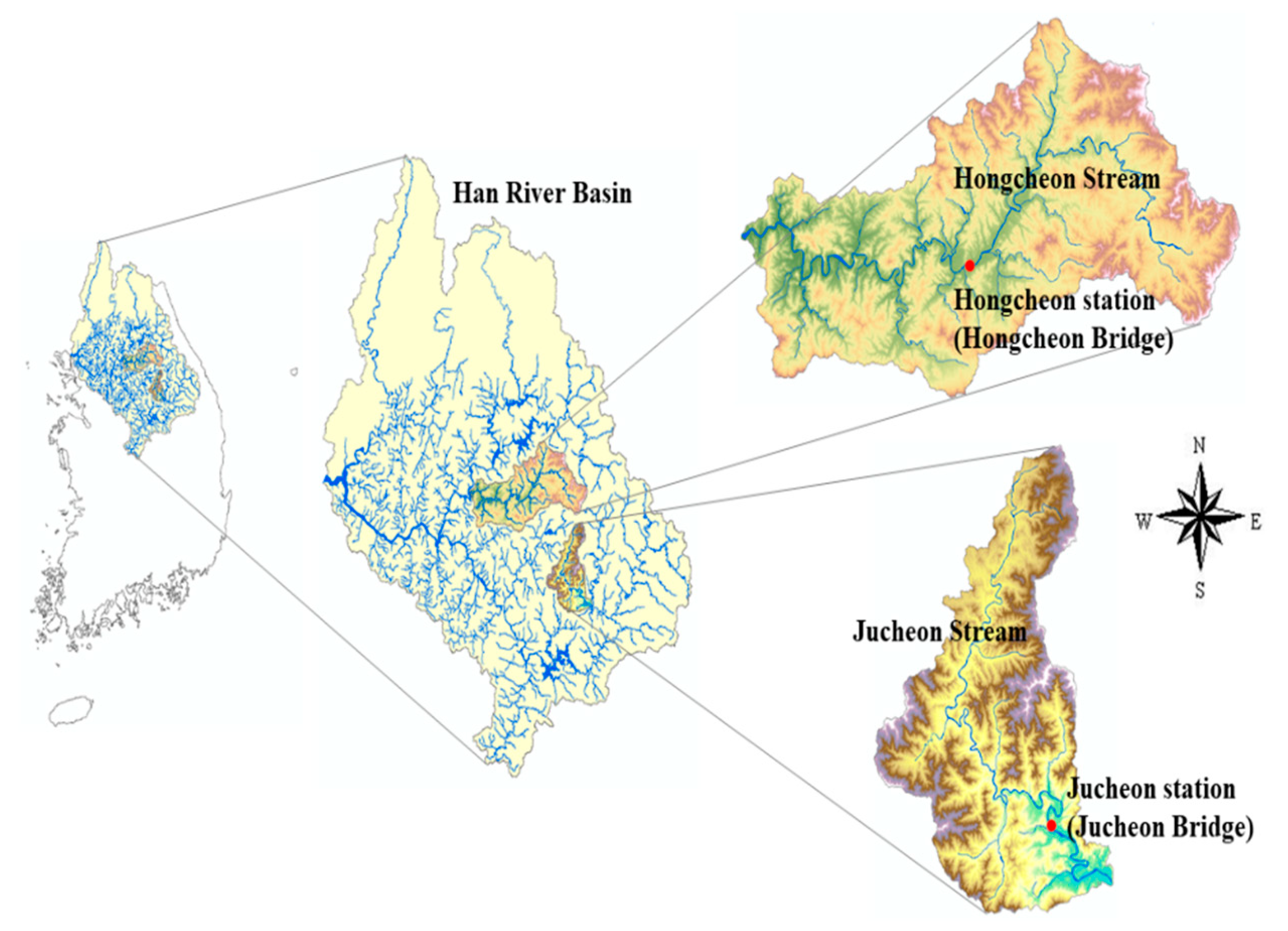
3. Study Area and Data

Under the addressed research, two stations (i.e., Hongcheon and Jucheon) were appointed for forecasting streamflow of the Hongcheon and Jucheon Streams (e.g., branches of the Han River), South Korea. Hongcheon station is located at Hongcheon Bridge with a latitude of 37°41′ N and a longitude of 127°52′ E, and Jucheon station is located at Jucheon Bridge with a latitude of 37°16′ N and a longitude of 128°15′ E, respectively.

Streamflow data in both stations have been collected and managed in the Water Resources Management Information System (WAMIS) of South Korea. The data available were divided into two phases: 80% (1 October 2003–30 September 2011) of the whole data was employed for the training phase and the remainder (i.e., 20%) (1 October 2011–30 September 2013) of the dataset was kept for the testing phase. The schematic diagrams of Hongcheon and Jucheon stations are provided in Figure 4. The properties of the used data for models’ development are summed up in

Table 1. Statistical properties of the streamflow data.

	Hongcheon		Jucheon
	Training	Testing	Training	Testing
Number	2922	731	2922	731
Maximum	1951.5	1362	2720.4	515.5
Minimum	2.92	0.92	0.01	1.12
Average	67.245	32.552	27.519	16.203
Standard Deviation	111.949	83.321	105.677	39.099
Skewness	4.844	9.310	11.966	7.207

. The statistical evidence that the streamflow data have highly skewed distributions indicates the chaotic behavior of the studied data. Since the streamflow follows a complicated transformation of excess rainfall, surface, and subsurface flows, Salas et al. [60] reported that the streamflow bounced off chaotic behavior with low dimension for the outlet of specific watershed.

One of the important projects for streamflow forecasting is determination of the appropriate input variables [1,27]. For the application of forecasting model, the optimal selection of the best input combination based on the antecedent times was suggested using six different combinations. The detection of appropriate antecedent times for streamflow forecasting can be clarified as identification of catchment characteristics including area, shape, length, and slope, etc. The previous research demonstrated that the recent antecedent times (e.g., (t − 1), (t − 2), and (t − 3)) were better associated than the ancient ones [27,61]. Rezaie-Balf et al. [27] accomplished that the antecedent times for daily streamflow forecasting were determined as (t − 1)~(t − 4) days in Tajan (Iran) and Hongcheon (South Korea) rivers. Under the addressed study, the antecedent times were increased to verify the effective outcomes (e.g., forecasting accuracy) of input combinations based on the article of [27]. Thus, the six input combinations (i.e., six categories from M1 to M6) using six antecedent times values which are provided in

Table 2. Different input combinations for streamflow forecasting.

Types	Input Combinations	Functions
M1	t − 1	Q(t) = f (Q(t − 1))
M2	t − 1, t − 2	Q(t) = f (Q(t − 1), Q(t − 2))
M3	t − 1, t − 2, t − 3	Q(t) = f (Q(t − 1), Q(t − 2), Q(t − 3))
M4	t − 1, t − 3, t − 5	Q(t) = f (Q(t − 1), Q(t − 3), Q(t − 5))
M5	t − 2, t − 4, t − 6	Q(t) = f (Q(t − 2), Q(t − 4), Q(t − 6))
M6	t − 1, t − 2, t − 3, t − 4, t − 5, t − 6	Q(t) = f (Q(t − 1), Q(t − 2), Q(t − 3), Q(t − 4), Q(t − 5), Q(t − 6))

were employed for the implemented methods.

4. Application and Results

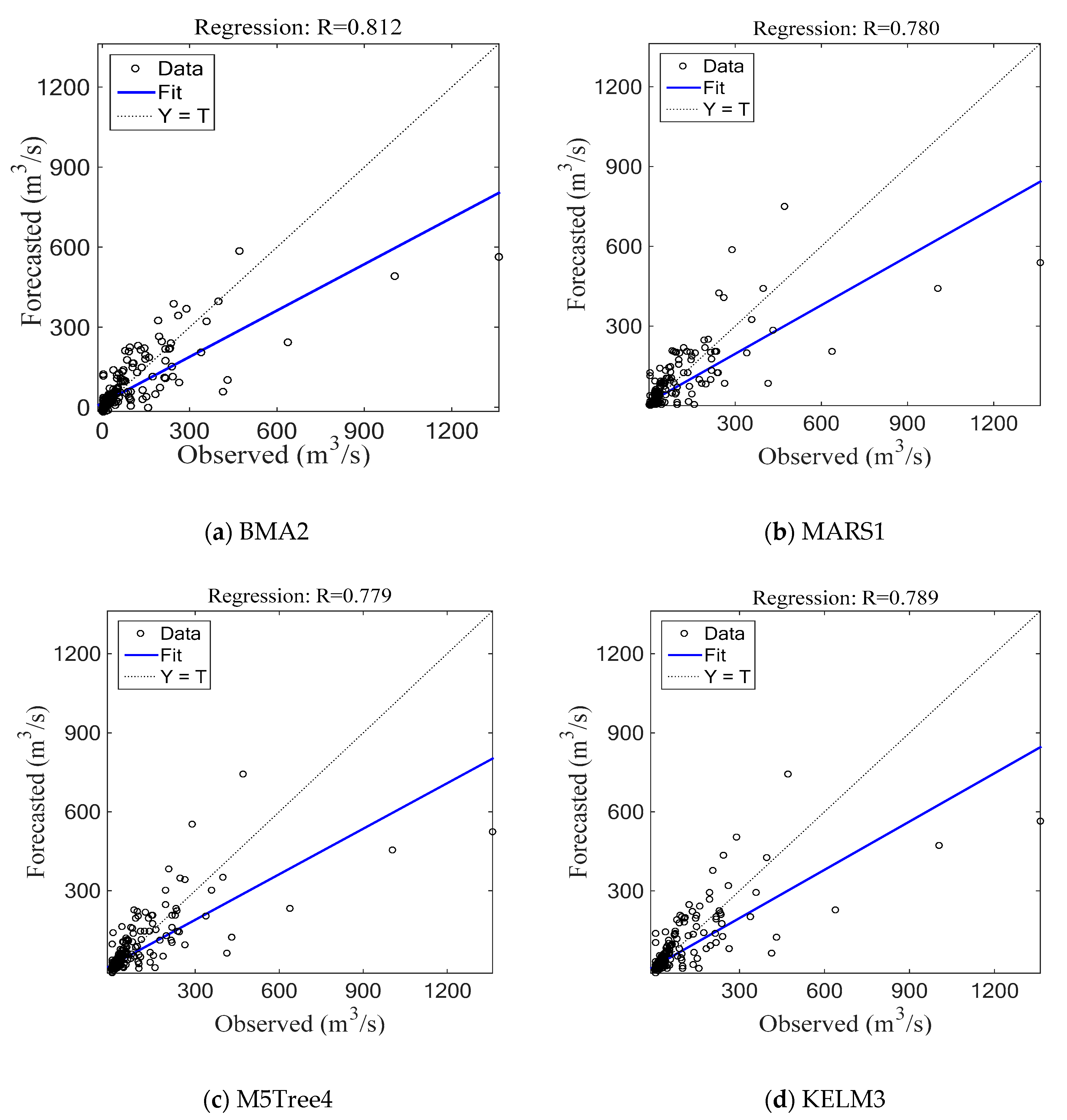
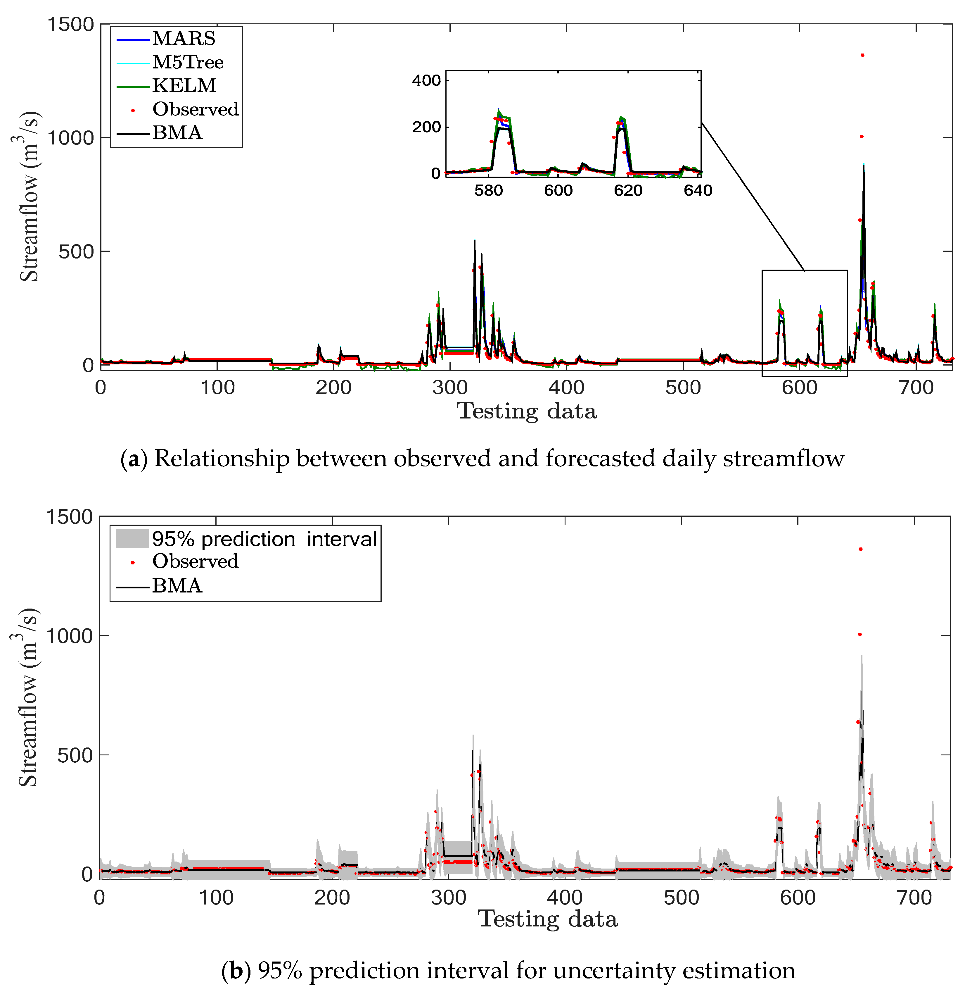
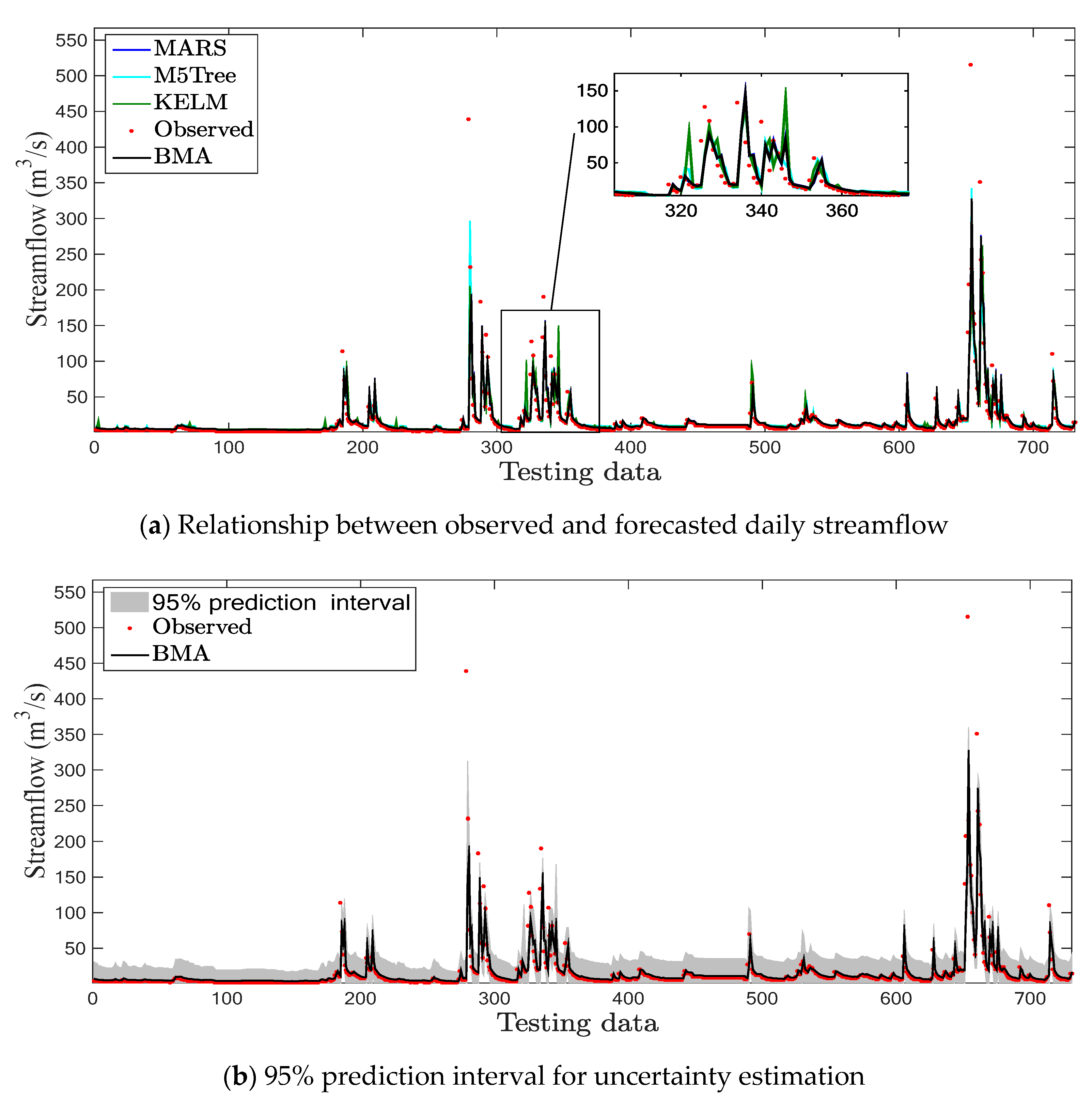
4.1. Hongcheon Station

Forecasting accuracy of developed models during testing phase are provided in

Table 3. Performance of MARS, M5Tree, KELM, and Bayesian model averaging (BMA) models in terms of root mean square error (RMSE), Nash-Sutcliffe Efficiency (NSE), correlation coefficient ®, and mean absolute error (MAE) values during testing phase (Hongcheon station).

Category	Assessment Indexes	MARS1	M5Tree1	KELM1	BMA1
	RMSE (m3/s)	52.214	52.866	51.541	50.887
M1	NSE	0.609	0.600	0.619	0.629
	R	0.780	0.780	0.789	0.798
	MAE (m3/s)	15.510	14.860	15.890	19.280
		MARS2	M5Tree2	KELM2	BMA2
	RMSE (m3/s)	56.026	55.442	55.160	49.507
M2	NSE	0.550	0.560	0.564	0.649
	R	0.743	0.749	0.751	0.812
	MAE (m3/s)	16.210	15.160	14.740	17.200
		MARS3	M5Tree3	KELM3	BMA3
	RMSE (m3/s)	54.280	57.704	51.242	50.212
M3	NSE	0.578	0.523	0.624	0.639
	R	0.760	0.732	0.789	0.805
	MAE (m3/s)	15.500	14.320	13.470	15.010
		MARS4	M5Tree4	KELM4	BMA4
	RMSE (m3/s)	58.394	52.528	53.611	49.933
M4	NSE	0.511	0.605	0.588	0.643
	R	0.715	0.779	0.767	0.808
	MAE (m3/s)	16.110	15.720	14.080	14.720
		MARS5	M5Tree5	KELM5	BMA5
	RMSE (m3/s)	71.612	72.264	69.496	69.283
M5	NSE	0.266	0.252	0.308	0.313
	R	0.524	0.505	0.555	0.562
	MAE (m3/s)	26.860	23.910	21.360	25.040
		MARS6	M5Tree6	KELM6	BMA6
	RMSE (m3/s)	54.154	58.372	51.473	51.212
M6	NSE	0.580	0.512	0.620	0.624
	R	0.762	0.715	0.794	0.790
	MAE (m3/s)	15.570	16.310	15.690	14.410

for Hongcheon station. Bold values indicate the best category of each model (i.e., MARS, M5Tree, KELM, and BMA). The MARS1 model (RMSE = 52.214 m³/s and NSE = 0.609) suggested the best performance among all the MARS models. Additionally, the M5Tree4 model (RMSE = 52.528 m³/s and NSE = 0.605) provided the best achievement among all the M5Tree models. Besides, the KELM3 model (RMSE = 51.242 m³/s and NSE = 0.624) supported the best accomplishment among all the KELM models. Finally, the BMA2 model (RMSE = 49.507 m³/s and NSE = 0.649) furnished the best accuracy among all the BMA models for streamflow forecasting. Additionally, it can be found from Table 3 that the BMA models provided better performance than the MARS, M5Tree, and KELM models based on each category (i.e., Categories M1–M6) during testing phase. Therefore, the BMA2 (i.e., having t − 1 and t − 2 antecedent times) model supplied the best forecasting accuracy compared to the other models, whereas the M5-based models (i.e., MARS5, M5Tree5, KELM5, and BMA5) showed the worst performance considering all models and categories.

The scatter diagrams between the observed and forecasted streamflow values using the best models (i.e., MARS1, M5Tree4, KELM3, and BMA2) based on each model (i.e., MARS, M5Tree, KELM, and BMA) and category for Hongcheon station are illustrated in Figure 5a–d including the exact (y = x) line, fitted line, and R value, respectively. It can be judged that the forecasted streamflow values based on the BMA2 model were more adjacent to the equivalent observed values during testing phase. Figure 6 supports the RMSE values for each model during testing phase in Hongcheon station. It can be observed from Figure 6 that the BMA models based on M1–M6 categories provided lower RMSE compared to other models during testing phase.

Figure 7a,b present the comparison of methods in streamflow forecasting based on M2 category during testing phase in Hongcheon station. It can be judged from Figure 7a that the BMA2 model forecasted the observed streamflow closely compared to other models (i.e., MARS2, M5Tree2, and KELM2). Additionally, Figure 7b explains the uncertainty estimation using 95% prediction interval for the BMA2 model. It can be found from Figure 7b that the BMA2 model provided higher uncertainty of peak flows compared to that of low flows.

In addition, Figure 8a,b provide that the comparison of streamflows based on M4 category during testing phase in Hongcheon station. Furthermore, it can be seen from Figure 8a that the BMA4 model better forecasted the observed streamflow than the alternative models (i.e., MARS4, M5Tree4, and KELM4). Additionally, Figure 8b represents the uncertainty estimation using 95% prediction interval for the BMA4 model. It can be seen from Figure 8b that the BMA4 model has also higher uncertainty in catching peak flows compared to that of low flows.

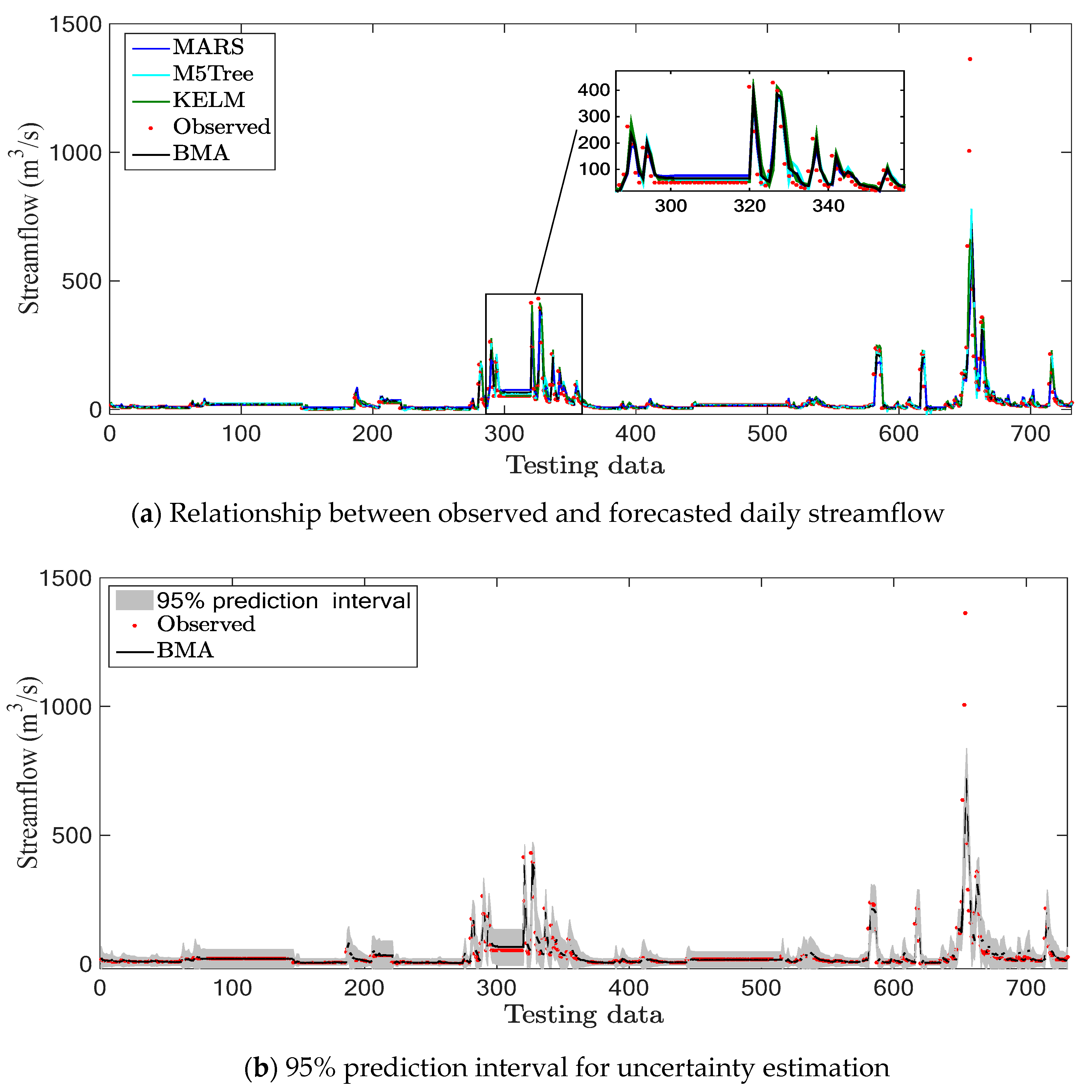
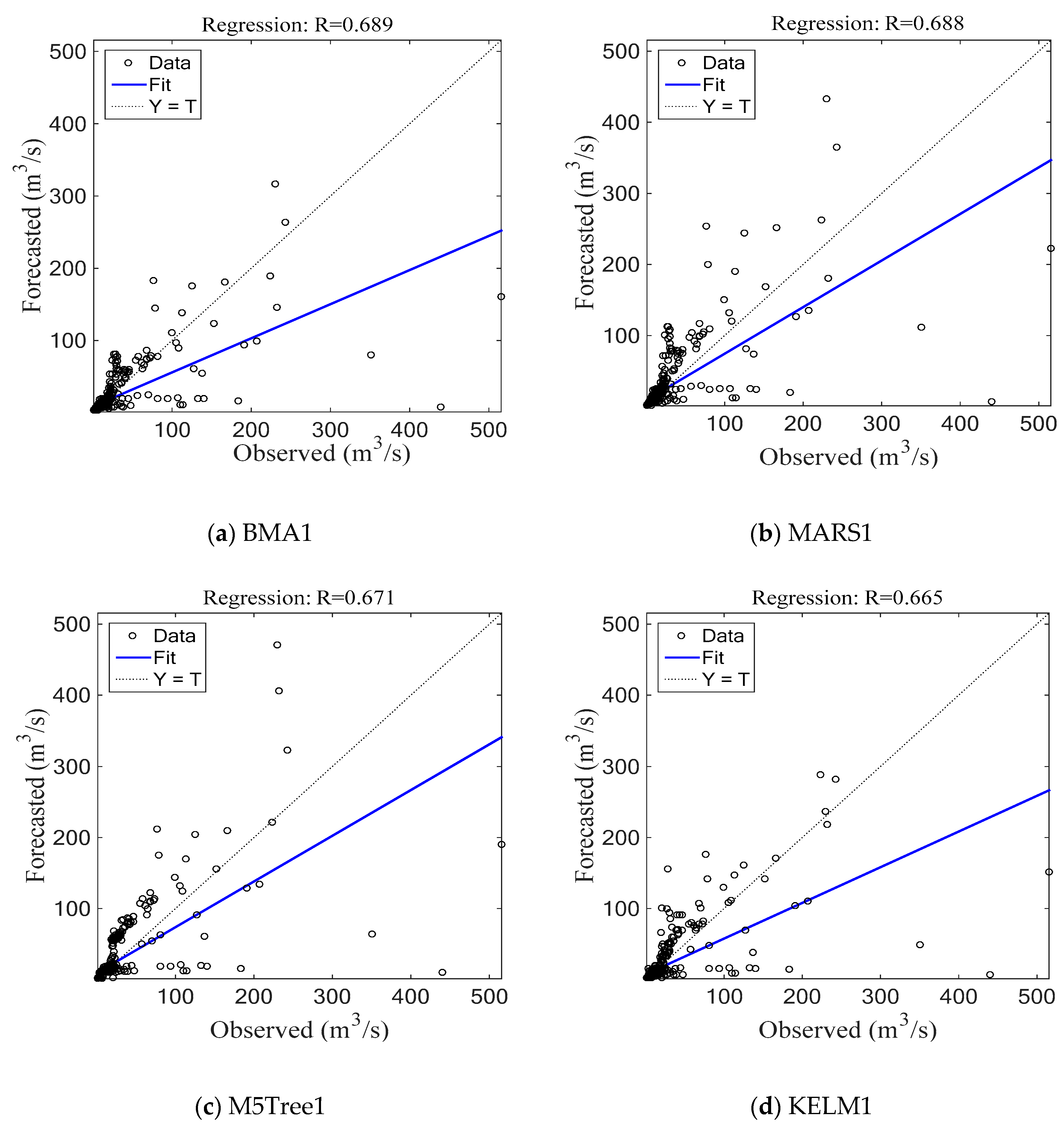
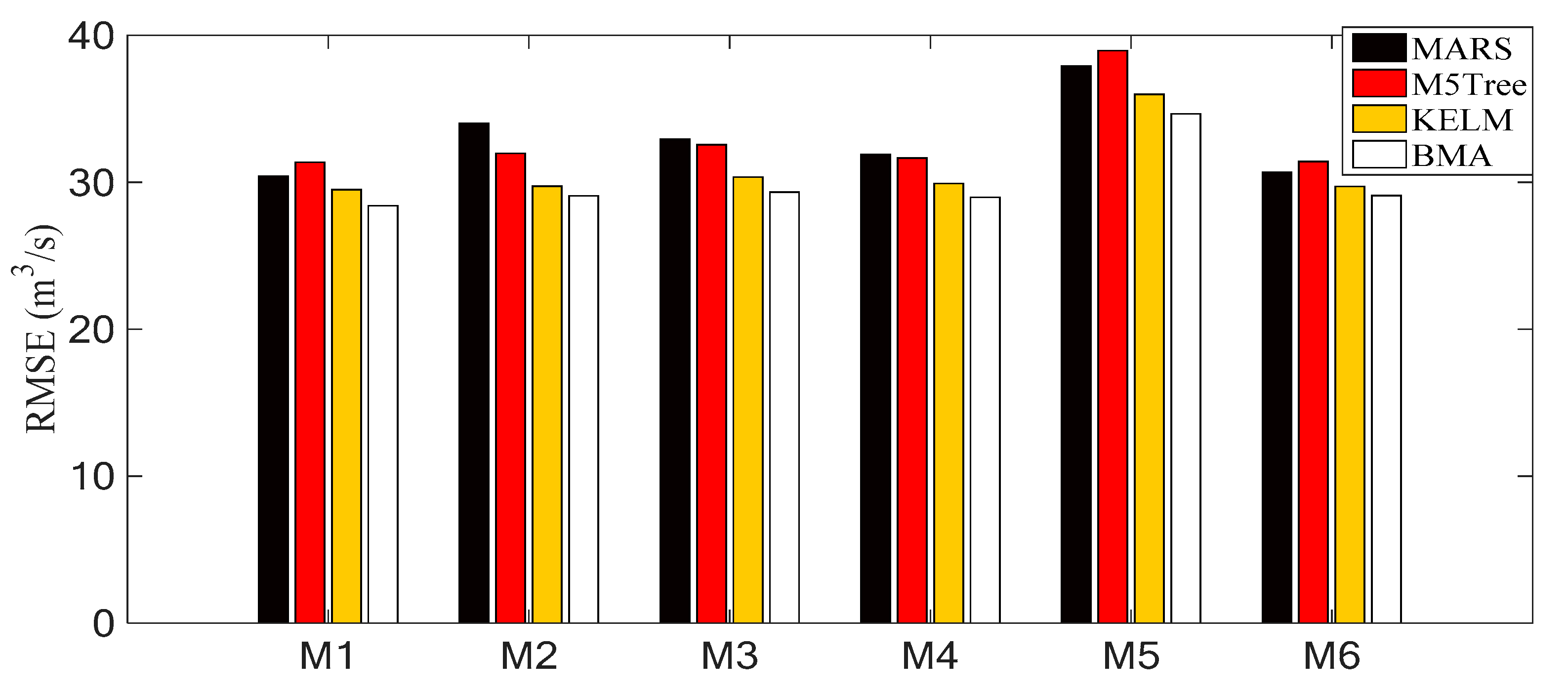
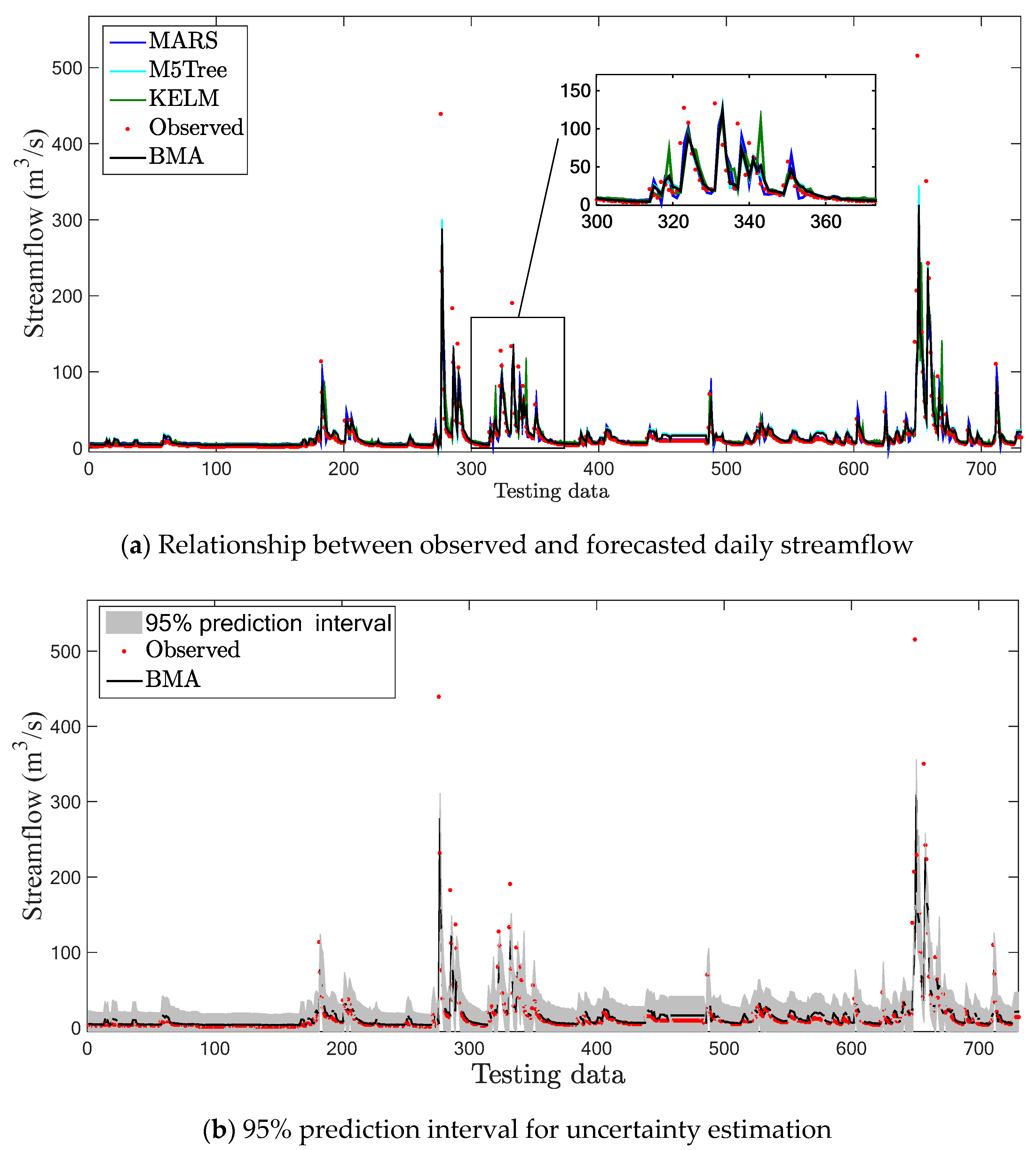
4.2. Jucheon Station

Table 4. Performance of MARS, M5Tree, KELM, and BMA models in terms of RMSE, NSE, and R values during testing phase (Jucheon station).

Category	Assessment Indexes	MARS1	M5Tree1	KELM1	BMA1
	RMSE (m3/s)	30.429	31.367	29.498	28.396
M1	NSE	0.397	0.360	0.434	0.475
	R	0.688	0.670	0.664	0.689
	MAE (m3/s)	9.910	10.390	7.380	7.850
		MARS2	M5Tree2	KELM2	BMA2
	RMSE (m3/s)	34.026	31.972	29.730	29.083
M2	NSE	0.247	0.335	0.425	0.449
	R	0.642	0.654	0.667	0.670
	MAE (m3/s)	10.760	9.900	7.600	7.840
		MARS3	M5Tree3	KELM3	BMA3
	RMSE (m3/s)	32.925	32.554	30.346	29.321
M3	NSE	0.294	0.310	0.401	0.440
	R	0.656	0.658	0.648	0.664
	MAE (m3/s)	10.490	13.180	7.700	7.940
		MARS4	M5Tree4	KELM4	BMA4
	RMSE (m3/s)	31.896	31.648	29.923	28.972
M4	NSE	0.337	0.347	0.416	0.454
	R	0.654	0.665	0.651	0.674
	MAE (m3/s)	10.540	11.720	7.550	7.990
		MARS5	M5Tree5	KELM5	BMA5
	RMSE (m3/s)	37.917	38.960	35.990	34.657
M5	NSE	0.063	0.011	0.156	0.219
	R	0.465	0.415	0.445	0.469
	MAE (m3/s)	15.410	19.110	11.960	11.870
		MARS6	M5Tree6	KELM6	BMA6
	RMSE (m3/s)	30.690	31.417	29.723	29.092
M6	NSE	0.386	0.357	0.424	0.449
	R	0.676	0.651	0.656	0.670
	MAE (m3/s)	9.730	11.800	7.610	8.190

supplies the forecasted accuracy of employed models during testing phase in Jucheon station. Bold values display the best category of each model (i.e., MARS, M5Tree, KELM, and BMA). M1-based models (RMSE = 30.429 m³/s and NSE = 0.397 in MARS1; RMSE = 31.367 m³/s and NSE = 0.360 in M5Tree1; RMSE = 29.498 m³/s and NSE = 0.434 in KELM1; RMSE = 28.396 m³/s and NSE = 0.475 in BMA1) suggested the best accuracy based on each category (i.e., Categories M1–M6) for streamflow forecasting. Additionally, it can be seen from Table 4 that the BMA model provided better forecasting ability than the MARS, M5Tree, and KELM models considering each category. Based on all models and categories, the BMA1 (i.e., having t − 1 antecedent time) model furnished the best forecasting compared to the other models, while the worst accuracy was accomplished by the M5-based models during testing phase in Jucheon station.

Considering all models and categories, the observed and forecasted streamflow values using the best models (i.e., MARS1, M5Tree1, KELM1, and BMA1) are illustrated in Figure 9a–d including the exact (y = x) line, fitted line, and R value for Jucheon station, respectively. It can be seen that the forecasted streamflow values based on BMA1 model were more neighboring to the corresponding observed values during testing phase. Figure 10 explains the RMSE values for each model during testing phase in Jucheon station. It can be seen from the figure that the BMA models based on M1–M6 categories provided lower RMSE compared to other models.

Figure 11a,b present the comparison of methods in streamflow forecasting based on M1 category during testing phase in Jucheon station. It can be seen in Figure 11a that the BMA1 model provided better forecasting performance compared to other models (i.e., MARS1, M5Tree1, and KELM1). Additionally, Figure 11b explains the uncertainty estimation using 95% prediction interval for the BMA1 model. It can be considered from Figure 11b that the BMA1 model provided higher uncertainty of peak flows compared to that of low flows. Besides, Figure 12a,b yields the comparison of methods based on M4 category during testing phase in Jucheon station. It can be seen from Figure 12a that the BMA4 model produced better forecasting compared to other models (i.e., MARS4, M5Tree4, and KELM4). Additionally, Figure 12b describes the uncertainty estimation using 95% prediction interval for the BMA4 model. It can be considered from Figure 12b that the BMA4 model provided higher uncertainty for catching peak flows compared to that of low flows.

4.3. Discussion

The addressed research boosted that the BMA models based on each category correctly captured the nonlinear time series of streamflow and could carry out the accurate forecasting in both stations. The comparison of individual RMSE values among the best models in Hongcheon station supplied that the BMA2 model enhanced the accomplishment by 5.2%, 5.8%, and 3.4% compared to MARS1, M5Tree4, and KELM3 models during testing phase, respectively. Additionally, the comparison of individual RMSE values among the best models in Jucheon station furnished that the BMA1 model increased an efficiency by 6.7% (MARS1 model), 9.5% (M5Tree1 model), and 3.7% (KELM1 model) during testing phase.

Based on the category of the best models, the forecasted accuracy using the BMA model in Hongcheon and Jucheon stations was found to be slightly better than the other models. In addition, the best models in the Hongcheon station could be found considering the different category (i.e., MARS1, M5Tree4, KELM3, and BMA2 models), whereas the best models in the Jucheon station were discovered based on the M1 category (i.e., MARS1, M5Tree1, KELM1, and BMA1) during testing phase, respectively. The improvement difference between both stations might be derived from the characteristics (e.g., maximum and minimum values) of data available. The similar results can be found from the previous documents [2,62,63]. Additionally, comparison of two stations revealed that the employed models were more successful in forecasting streamflows of Jucheon station compared to Hongcheon station. This can be explained by the different properties of the data sets, for example, training data of Jucheon station have much more skewed distribution (skewness = 11.966, Table 1) than those of the other station. If the different models produced the best accuracy using the same data, the additional statistical skills (e.g., null hypothesis [64] and Akaike’s information criterion [65]) are proposed to determine the best model for the undergoing project. Considering the previous researches for Bayesian approaches, Rasouli et al. [62] proposed that three machine learning models (i.e., Bayesian neural network (BNN), support vector regression (SVR), and Gaussian process (GP)) were utilized to forecast the daily streamflow using from 1- to 7-day lead time, British Columbia, Canada. The BNN model outperformed other models slightly. Wang et al. [35] proved that the BMA–ensemble–wavelet–Volterra model were superior to the wavelet–Volterra and ensemble–wavelet–Volterra models, obviously. Therefore, the forecasting accuracy of addressed research follows the previous researches.

As one of the continuous projects for streamflow forecasting, the different forecasting models (e.g., seasonal autoregressive integrated moving average (SARIMA) [66,67] and bootstrap aggregation (bagging) [68]), which demonstrated their superiority for temporal forecasting in previous literature, can be applied to compare and evaluate the performance accuracy of BMA model. In addition, different nature-inspired evolutionary algorithms and data pre-processing approaches can be joined with the BMA model to increase the forecasting accuracy of hydrological processes including streamflow, water stage, and groundwater, etc. Thus, to boost the forecasting accuracy of undergoing project, the continuous researches utilizing the BMA model, evolutionary algorithms, and data pre-processing techniques should be recommended for daily streamflow forecasting.

5. Conclusions

Accurate streamflow forecasting is a major problem of interest related to water resources and hydrology. This research evaluated the efficiency of Bayesian model averaging (BMA) model for daily streamflow forecasting in two different streams including Hongcheon and Jucheon stations, South Korea. Six categories (i.e., M1–M6) of input combination using different antecedent times were employed for streamflow forecasting. Additionally, the forecasting accuracy of the BMA model were compared with those of other models (i.e., MARS, M5Tree, and KELM) with respect to root mean square error (RMSE), Nash-Sutcliff efficiency (NSE), correlation coefficient (R), and mean absolute error (MAE).

The forecasting accuracy confirmed that the best BMA model (i.e., BMA2) increased an achievement by 5.2% (MARS1 model), 5.8% (M5Tree4 model), and 3.4% (KELM3 model) based on RMSE values among the best models during testing phase in Hongcheon station. Additionally, the best BMA model (i.e., BMA1) enhanced an accuracy by 6.7% (MARS1 model), 9.5% (M5Tree1 model), and 3.7% (KELM1 model) based on the best models during testing phase in Jucheon station. In addition, the best BMA models (i.e., BMA2 in Hongcheon station and BMA1 in Jucheon station) permitted the uncertainty estimation, and accomplished higher uncertainty of peak flows compared to that of low flows.

The addressed research outcomes suggested that the BMA model could be successfully employed for streamflow forecasting with different antecedent times for sustainable and efficient water management. For the continuous research, the different hybrid approaches such as coupling BMA model, evolutionary algorithm, and data pre-processing, can be recommended as a potential alternative methodology to enhance the forecasting accuracy based on diverse hydrological processes.

References

1. Seo, Y.; Kim, S.; Kisi, O.; Singh, V.P. Daily water level forecasting using wavelet decomposition and artificial intelligence techniques. J. Hydrol. 2015, 520, 224–243. [Google Scholar] [CrossRef]
2. Yaseen, Z.M.; Jaafar, O.; Deo, R.C.; Kisi, O.; Adamowski, J.; Quilty, J.; El-Shafie, A. Stream-flow forecasting using extreme learning machines: A case study in a semi-arid region in Iraq. J. Hydrol. 2016, 542, 603–614. [Google Scholar] [CrossRef]
3. Zakhrouf, M.; Bouchelkia, H.; Stamboul, M.; Kim, S. Novel hybrid approaches based on evolutionary strategy for streamflow forecasting in the Chellif River, Algeria. Acta Geophys. 2020, 68, 167–180. [Google Scholar] [CrossRef]
4. Zakhrouf, M.; Bouchelkia, H.; Stamboul, M.; Kim, S.; Singh, V.P. Implementation on the evolutionary machine learning approaches for streamflow forecasting: Case study in the Seybous River, Algeria. J. Korea Water Resour. Assoc. 2020, 53, 395–408. [Google Scholar]
5. Badrzadeh, H.; Sarukkalige, R.; Jayawardena, A.W. Intermittent stream flow forecasting and modelling with hybrid wavelet neuro-fuzzy model. Hydrol. Res. 2018, 49, 27–40. [Google Scholar] [CrossRef]
6. Zhou, J.; Peng, T.; Zhang, C.; Sun, N. Data pre-analysis and ensemble of various artificial neural networks for monthly streamflow forecasting. Water 2018, 10, 628. [Google Scholar] [CrossRef] [Green Version]
7. Tikhamarine, Y.; Souag-Gamane, D.; Ahmed, A.N.; Kisi, O.; El-Shafie, A. Improving artificial intelligence models accuracy for monthly streamflow forecasting using grey Wolf optimization (GWO) algorithm. J. Hydrol. 2020, 582, 124435. [Google Scholar] [CrossRef]
8. Yaseen, Z.M.; Allawi, M.F.; Yousif, A.A.; Jaafar, O.; Hamzah, F.M.; El-Shafie, A. Non-tuned machine learning approach for hydrological time series forecasting. Neural. Comput. Appl. 2018, 30, 1479–1491. [Google Scholar] [CrossRef]
9. Luo, X.; Yuan, X.; Zhu, S.; Xu, Z.; Meng, L.; Peng, J. A hybrid support vector regression framework for streamflow forecast. J. Hydrol. 2019, 568, 184–193. [Google Scholar] [CrossRef]
10. Cheng, M.; Fang, F.; Kinouchi, T.; Navon, I.M.; Pain, C.C. Long lead-time daily and monthly streamflow forecasting using machine learning methods. J. Hydrol. 2020, 590, 125376. [Google Scholar] [CrossRef]
11. Yu, X.; Wang, Y.; Wu, L.; Chen, G.; Wang, L.; Qin, H. Comparison of support vector regression and extreme gradient boosting for decomposition-based data-driven 10-day streamflow forecasting. J. Hydrol. 2020, 582, 124293. [Google Scholar] [CrossRef]
12. Papacharalampous, G.A.; Tyralis, H. Evaluation of random forests and prophet for daily streamflow forecasting. Adv. Geosci. 2018, 45, 201–208. [Google Scholar] [CrossRef] [Green Version]
13. Rezaie-Balf, M.; Kisi, O. New formulation for forecasting streamflow: Evolutionary polynomial regression vs. extreme learning machine. Hydrol. Res. 2018, 49, 939–953. [Google Scholar] [CrossRef] [Green Version]
14. Zakhrouf, M.; Bouchelkia, H.; Stamboul, M.; Kim, S.; Heddam, S. Time series forecasting of river flow using an integrated approach of wavelet multi-resolution analysis and evolutionary data-driven models. A case study: Sebaou River (Algeria). Phys. Geogr. 2018, 39, 506–522. [Google Scholar] [CrossRef]
15. Li, F.F.; Wang, Z.Y.; Qiu, J. Long-term streamflow forecasting using artificial neural network based on preprocessing technique. J. Forecast. 2019, 38, 192–206. [Google Scholar] [CrossRef]
16. Fu, M.; Fan, T.; Ding, Z.A.; Salih, S.Q.; Al-Ansari, N.; Yaseen, Z.M. Deep learning data-intelligence model based on adjusted forecasting window scale: Application in daily streamflow simulation. IEEE Access 2020, 8, 32632–32651. [Google Scholar] [CrossRef]
17. Al-Sudani, Z.A.; Salih, S.Q.; Yaseen, Z.M. Development of multivariate adaptive regression spline integrated with differential evolution model for streamflow simulation. J. Hydrol. 2019, 573, 1–12. [Google Scholar] [CrossRef]
18. Adamowski, J.; Chan, H.F.; Prasher, S.O.; Sharda, V.N. Comparison of multivariate adaptive regression splines with coupled wavelet transform artificial neural networks for runoff forecasting in Himalayan micro-watersheds with limited data. J. Hydroinformatics 2012, 14, 731–744. [Google Scholar] [CrossRef]
19. Tyralis, H.; Papacharalampous, G.; Langousis, A. Super ensemble learning for daily streamflow forecasting: Large-scale demonstration and comparison with multiple machine learning algorithms. Neural. Comput. Appl. 2020, 1–16. [Google Scholar] [CrossRef]
20. Solomatine, D.P.; Xue, Y. M5 model trees and neural networks: Application to flood forecasting in the upper reach of the Huai River in China. J. Hydrol. Eng. 2004, 9, 491–501. [Google Scholar] [CrossRef]
21. Štravs, L.; Brilly, M. Development of a low-flow forecasting model using the M5 machine learning method. Hydrol. Sci. J. 2007, 52, 466–477. [Google Scholar] [CrossRef]
22. Sattari, M.T.; Pal, M.; Apaydin, H.; Ozturk, F. M5 model tree application in daily river flow forecasting in Sohu Stream, Turkey. Water Resour. 2013, 40, 233–242. [Google Scholar] [CrossRef]
23. Adnan, R.M.; Yuan, X.; Kisi, O.; Adnan, M.; Mehmood, A. Stream flow forecasting of poorly gauged mountainous watershed by least square support vector machine, fuzzy genetic algorithm and M5 model tree using climatic data from nearby station. Water Resour. Manag. 2018, 32, 4469–4486. [Google Scholar] [CrossRef]
24. Yaseen, Z.M.; Kisi, O.; Demir, V. Enhancing long-term streamflow forecasting and predicting using periodicity data component: Application of artificial intelligence. Water Resour. Manag. 2016, 30, 4125–4151. [Google Scholar] [CrossRef]
25. Yin, Z.; Feng, Q.; Wen, X.; Deo, R.C.; Yang, L.; Si, J.; He, Z. Design and evaluation of SVR, MARS and M5Tree models for 1, 2 and 3-day lead time forecasting of river flow data in a semiarid mountainous catchment. Stoch. Environ. Res. Risk. Assess. 2018, 32, 2457–2476. [Google Scholar] [CrossRef]
26. Kisi, O.; Choubin, B.; Deo, R.C.; Yaseen, Z.M. Incorporating synoptic-scale climate signals for streamflow modelling over the Mediterranean region using machine learning models. Hydrol. Sci. J. 2019, 64, 1240–1252. [Google Scholar] [CrossRef]
27. Rezaie-Balf, M.; Kim, S.; Fallah, H.; Alaghmand, S. Daily river flow forecasting using ensemble empirical mode decomposition based heuristic regression models: Application on the perennial rivers in Iran and South Korea. J. Hydrol. 2019, 572, 470–485. [Google Scholar] [CrossRef]
28. Rezaie-Balf, M.; Naganna, S.R.; Kisi, O.; El-Shafie, A. Enhancing streamflow forecasting using the augmenting ensemble procedure coupled machine learning models: Case study of Aswan High Dam. Hydrol. Sci. J. 2019, 64, 1629–1646. [Google Scholar] [CrossRef]
29. Lima, A.R.; Cannon, A.J.; Hsieh, W.W. Forecasting daily streamflow using online sequential extreme learning machines. J. Hydrol. 2016, 537, 431–443. [Google Scholar] [CrossRef]
30. Yadav, B.; Ch, S.; Mathur, S.; Adamowski, J. Discharge forecasting using an online sequential extreme learning machine (OS-ELM) model: A case study in Neckar River, Germany. Measurement 2016, 92, 433–445. [Google Scholar] [CrossRef]
31. Niu, W.J.; Feng, Z.K.; Cheng, C.T.; Zhou, J.Z. Forecasting daily runoff by extreme learning machine based on quantum-behaved particle swarm optimization. J. Hydrol. Eng. 2018, 23, 04018002. [Google Scholar] [CrossRef]
32. Vrugt, J.A.; Robinson, B.A. Treatment of uncertainty using ensemble methods: Comparison of sequential data assimilation and Bayesian model averaging. Water Resour. Res. 2007, 43, W01411. [Google Scholar] [CrossRef] [Green Version]
33. Duan, Q.; Ajami, N.K.; Gao, X.; Sorooshian, S. Multi-model ensemble hydrologic prediction using Bayesian model averaging. Adv. Water Resour. 2007, 30, 1371–1386. [Google Scholar] [CrossRef] [Green Version]
34. Jiang, S.; Ren, L.; Hong, Y.; Yong, B.; Yang, X.; Yuan, F.; Ma, M. Comprehensive evaluation of multi-satellite precipitation products with a dense rain gauge network and optimally merging their simulated hydrological flows using the Bayesian model averaging method. J. Hydrol. 2012, 452, 213–225. [Google Scholar] [CrossRef]
35. Wang, Q.J.; Schepen, A.; Robertson, D.E. Merging seasonal rainfall forecasts from multiple statistical models through Bayesian model averaging. J. Clim. 2012, 25, 5524–5537. [Google Scholar] [CrossRef]
36. Rathinasamy, M.; Adamowski, J.; Khosa, R. Multiscale streamflow forecasting using a new Bayesian Model Average based ensemble multi-wavelet Volterra nonlinear method. J. Hydrol. 2013, 507, 186–200. [Google Scholar] [CrossRef]
37. Liu, Z.; Merwade, V. Accounting for model structure, parameter and input forcing uncertainty in flood inundation modeling using Bayesian model averaging. J. Hydrol. 2018, 565, 138–149. [Google Scholar] [CrossRef]
38. Friedman, J. Multivariate adaptive regression splines. Ann. Stat. 1991, 19, 1–67. [Google Scholar] [CrossRef]
39. Zhang, W.G.; Goh, A.T.C. Multivariate adaptive regression splines for analysis of geotechnical engineering systems. Comput. Geotech. 2013, 48, 82–95. [Google Scholar] [CrossRef]
40. Solomatine, D.P.; Dulal, K.N. Model trees as an alternative to neural networks in rainfall—Runoff modelling. Hydrol. Sci. J. 2003, 48, 399–411. [Google Scholar] [CrossRef]
41. Loh, W.Y. Classification and regression trees. Wiley Interdiscip. Rev. Data Min. Knowl. Discov. 2011, 1, 14–23. [Google Scholar] [CrossRef]
42. Huang, G.B.; Zhu, Q.Y.; Siew, C.K. Extreme learning machine: Theory and applications. Neurocomputing 2006, 70, 489–501. [Google Scholar] [CrossRef]
43. Alizamir, M.; Kim, S.; Kisi, O.; Zounemat-Kermani, M. Deep echo state network: A novel machine learning approach to model dew point temperature using meteorological variables. Hydrol. Sci. J. 2020, 65, 1173–1190. [Google Scholar] [CrossRef]
44. Alizamir, M.; Kisi, O.; Ahmed, A.N.; Mert, C.; Fai, C.M.; Kim, S.; Kim, N.W.; El-Shafie, A. Advanced machine learning model for better prediction accuracy of soil temperature at different depths. PLoS ONE 2020, 15, e0231055. [Google Scholar] [CrossRef] [PubMed] [Green Version]
45. Huang, G.B.; Zhou, H.; Ding, X.; Zhang, R. Extreme learning machine for regression and multiclass classification. IEEE Trans. Syst. Man Cybern. Syst. 2012, 42, 513–529. [Google Scholar] [CrossRef] [PubMed] [Green Version]
46. Seo, Y.; Kim, S.; Singh, V.P. Comparison of different heuristic and decomposition techniques for river stage modeling. Environ. Monit. Assess 2018, 190, 392. [Google Scholar] [CrossRef] [PubMed]
47. Raftery, A.E.; Madigan, D.; Hoeting, J.A. Bayesian model averaging for linear regression models. J. Am. Stat. Assoc. 1997, 92, 179–191. [Google Scholar] [CrossRef]
48. Sloughter, J.M.L.; Raftery, A.E.; Gneiting, T.; Fraley, C. Probabilistic quantitative precipitation forecasting using Bayesian model averaging. Mon. Weather Rev. 2007, 135, 3209–3220. [Google Scholar] [CrossRef]
49. Kisi, O.; Alizamir, M.; Gorgij, A.D. Dissolved oxygen prediction using a new ensemble method. Environ. Sci. Pollut. Res. 2020, 27, 9589–9603. [Google Scholar] [CrossRef]
50. Kisi, O.; Alizamir, M.; Trajkovic, S.; Shiri, J.; Kim, S. Solar radiation estimation in Mediterranean climate by weather variables using a novel Bayesian model averaging and machine learning methods. Neural Process. Lett. 2020, 52, 2297–2318. [Google Scholar] [CrossRef]
51. Baran, S. Probabilistic wind speed forecasting using Bayesian model averaging with truncated normal components. Comput. Stat. Data Anal. 2014, 75, 227–238. [Google Scholar] [CrossRef] [Green Version]
52. Raftery, A.E.; Gneiting, T.; Balabdaoui, F.; Polakowski, M. Using Bayesian model averaging to calibrate forecast ensembles. Mon. Weather Rev. 2005, 133, 1155–1174. [Google Scholar] [CrossRef] [Green Version]
53. Willmott, C.J.; Matsuura, K. Advantages of the mean absolute error (MAE) over the root mean square error (RMSE) in assessing average model performance. Clim. Res. 2005, 30, 79–82. [Google Scholar] [CrossRef]
54. Dawson, C.W.; Abrahart, R.J.; See, L.M. HydroTest: A web-based toolbox of evaluation metrics for the standardised assessment of hydrological forecasts. Environ. Model. Softw. 2007, 22, 1034–1052. [Google Scholar] [CrossRef] [Green Version]
55. Deo, R.C.; Şahin, M.; Adamowski, J.F.; Mi, J. Universally deployable extreme learning machines integrated with remotely sensed MODIS satellite predictors over Australia to forecast global solar radiation: A new approach. Renew. Sust. Energ. Rev. 2019, 104, 235–261. [Google Scholar] [CrossRef]
56. Nash, J.E.; Sutcliffe, J.V. River flow forecasting through conceptual models, Part 1 – A discussion of principles. J. Hydrol. 1970, 10, 282–290. [Google Scholar] [CrossRef]
57. Wilcox, B.P.; Rawls, W.J.; Brakensiek, D.L.; Wight, J.R. Predicting runoff from rangeland catchments: A comparison of two models. Water Resour. Res. 1990, 26, 2401–2410. [Google Scholar] [CrossRef]
58. Legates, D.R.; McCabe, G.J. Evaluating the use of “goodness-of-fit” measures in hydrologic and hydroclimatic model validation. Water Resour. Res. 1999, 35, 233–241. [Google Scholar] [CrossRef]
59. Chai, T.; Draxler, R.R. Root mean square error (RMSE) or mean absolute error (MAE)?—Arguments against avoiding RMSE in the literature. Geosci. Model Dev. 2014, 7, 1247–1250. [Google Scholar] [CrossRef] [Green Version]
60. Salas, J.D.; Kim, H.S.; Eykholt, R.; Burlando, P.; Green, T.R. Aggregation and sampling in deterministic chaos: Implications for chaos identification in hydrological processes. Nonlinear Process. Geophys. 2005, 12, 557–567. [Google Scholar] [CrossRef] [Green Version]
61. Yaseen, Z.M.; El-Shafie, A.; Jaafar, O.; Afan, H.A.; Sayl, K.N. Artificial intelligence based models for stream-flow forecasting: 2000–2015. J. Hydrol. 2015, 530, 829–844. [Google Scholar] [CrossRef]
62. Rasouli, K.; Hsieh, W.W.; Cannon, A.J. Daily streamflow forecasting by machine learning methods with weather and climate inputs. J. Hydrol. 2012, 414, 284–293. [Google Scholar] [CrossRef]
63. Tongal, H.; Booij, M.J. Simulation and forecasting of streamflows using machine learning models coupled with base flow separation. J. Hydrol. 2018, 564, 266–282. [Google Scholar] [CrossRef]
64. McCuen, R.H. Microcomputer Applications in Statistical Hydrology, 1st ed.; Prentice Hall: Eaglewood Cliffs, NJ, USA, 1993; pp. 20–48. [Google Scholar]
65. Akaike, H. A new look at the statistical model identification. IEEE Trans. Automat. Contr. 1974, 19, 716–723. [Google Scholar] [CrossRef]
66. Thiyagarajan, K.; Kodagoda, S.; Ranasinghe, R.; Vitanage, D.; Iori, G. Robust sensor suite combined with predictive analytics enabled anomaly detection model for smart monitoring of concrete sewer pipe surface moisture conditions. IEEE Sens. J. 2020, 20, 8232–8243. [Google Scholar] [CrossRef]
67. Thiyagarajan, K.; Kodagoda, S.; Van Nguyen, L.; Ranasinghe, R. Sensor failure detection and faulty data accommodation approach for instrumented wastewater infrastructures. IEEE Access 2018, 6, 56562–56574. [Google Scholar] [CrossRef]
68. Melesse, A.M.; Khosravi, K.; Tiefenbacher, J.P.; Heddam, S.; Kim, S.; Mosavi, A.; Pham, B.T. River water salinity prediction using hybrid machine learning models. Water 2020, 12, 2951. [Google Scholar] [CrossRef]
Figure 1. Architecture of multivariate adaptive regression spline (MARS) model (M6 category).
Sustainability 12 09720 g001
Figure 2. Architecture of M5Tree model.
Sustainability 12 09720 g002
Figure 3. Architecture of ELM model (M6 category).
Sustainability 12 09720 g003
Figure 4. Schematic diagram of research area.
Sustainability 12 09720 g004
Figure 5. Scatter diagrams for the best models during testing phase (Hongcheon station).
Sustainability 12 09720 g005
Figure 6. Comparison of RMSE values for each model during testing phase (Hongcheon station).
Sustainability 12 09720 g006
Figure 7. Comparison of streamflow based on M2 category during testing phase (Hongcheon station).
Sustainability 12 09720 g007
Figure 8. Comparison of streamflow based on M4 category during testing phase (Hongcheon station).
Sustainability 12 09720 g008
Figure 9. Scatter diagrams for the best models during testing phase (Jucheon station).
Sustainability 12 09720 g009
Figure 10. Comparison of RMSE values for each model during testing phase (Jucheon station).
Sustainability 12 09720 g010
Figure 11. Comparison of streamflow based on M1 category during testing phase (Jucheon station).
Sustainability 12 09720 g011
Figure 12. Comparison of streamflow based on M4 category during testing phase (Jucheon station).
Sustainability 12 09720 g012